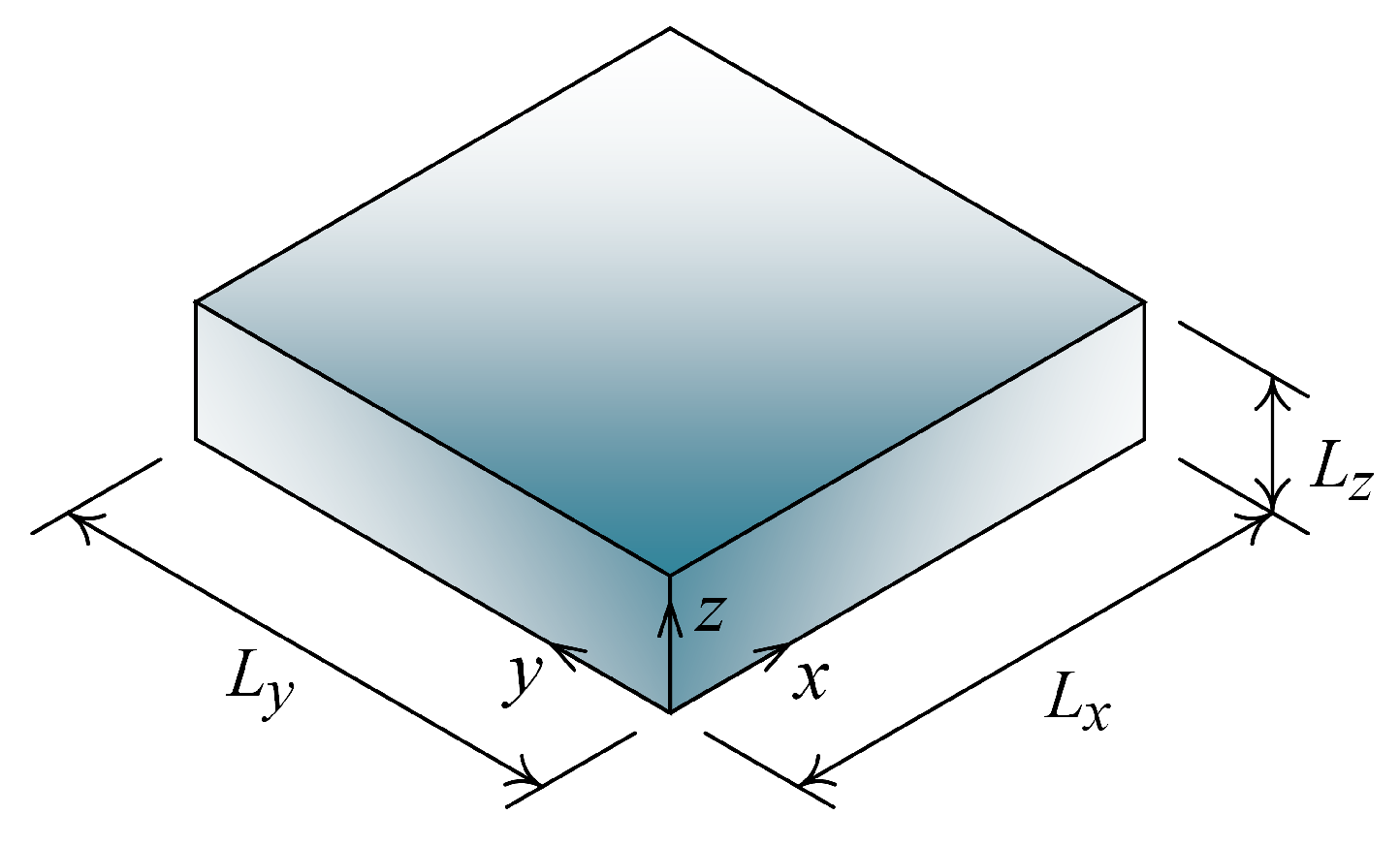
Figure 1.
Schematic representation of plate, coordinate system and their dimensions.
Figure 1.
Schematic representation of plate, coordinate system and their dimensions.
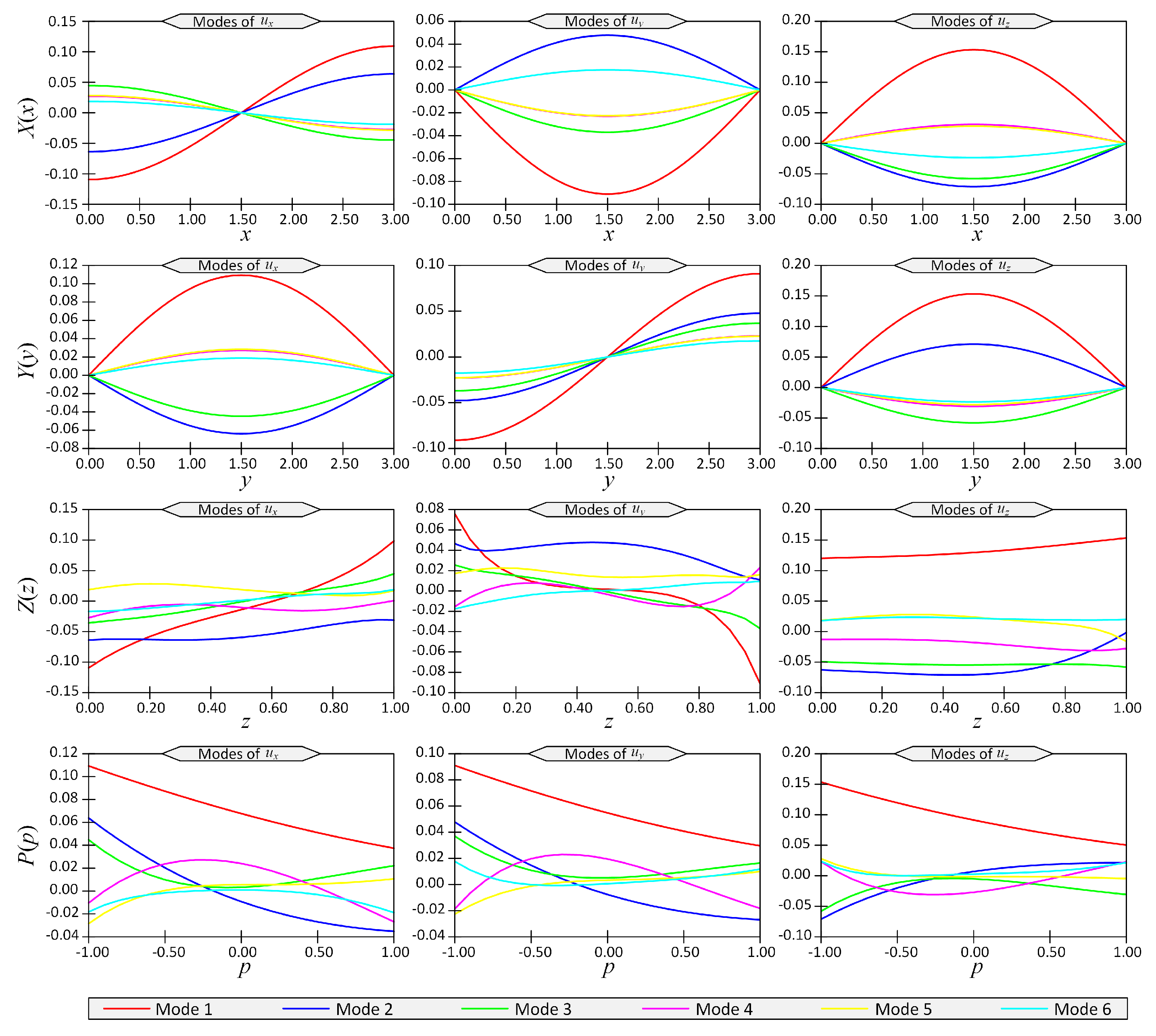
Figure 2.
The first six modes of displacement components () with respect to space coordinates () for Example 1 for boundary conditions case SSSS.
Figure 2.
The first six modes of displacement components () with respect to space coordinates () for Example 1 for boundary conditions case SSSS.
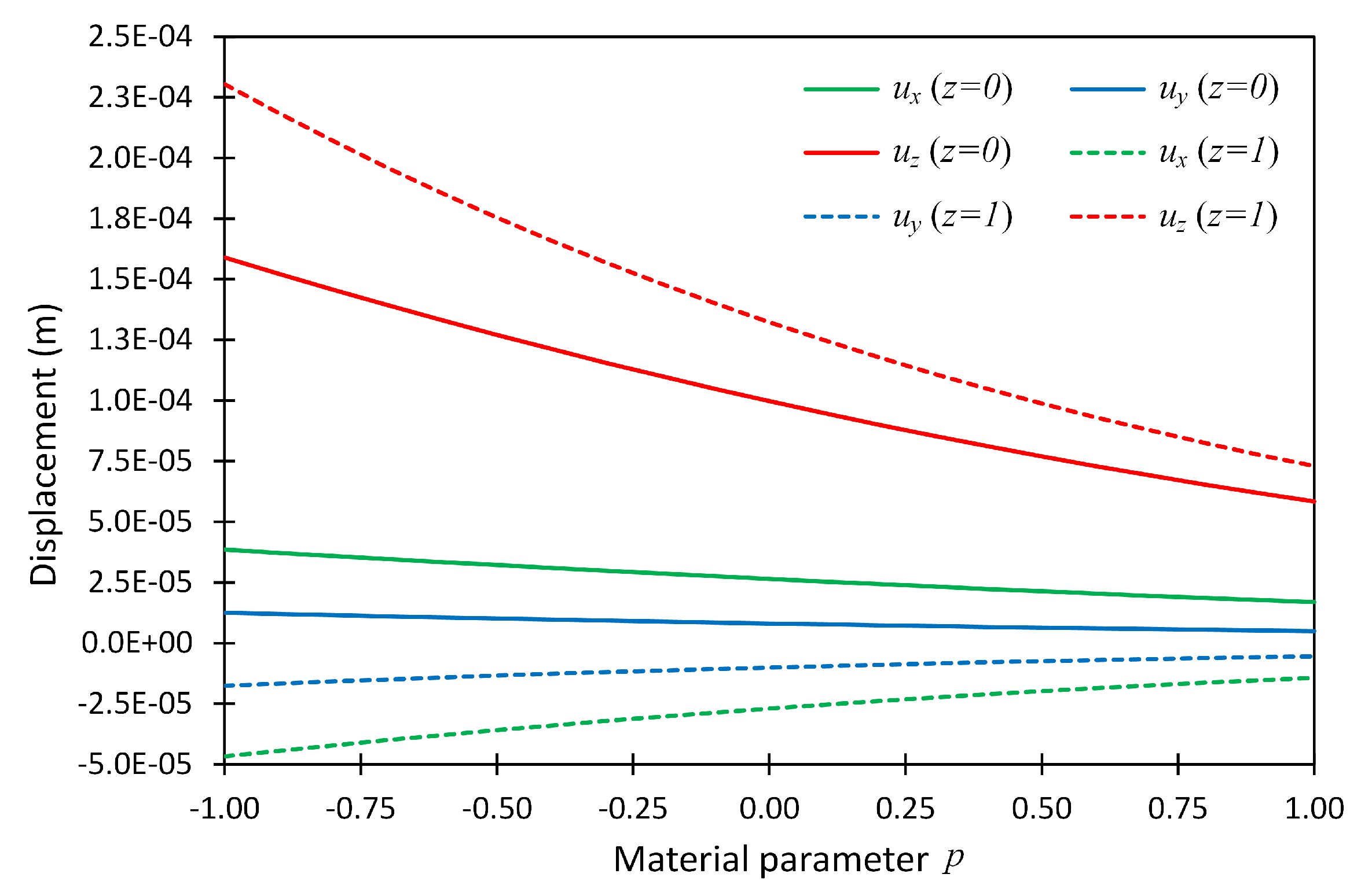
Figure 3.
The displacement components at two locations (
) = (
) and (
) versus material parameter
p for Example 1 considering boundary conditions SSSS; the reference solution given in (Pan 2003) [
24] is shown by solid dots.
Figure 3.
The displacement components at two locations (
) = (
) and (
) versus material parameter
p for Example 1 considering boundary conditions SSSS; the reference solution given in (Pan 2003) [
24] is shown by solid dots.
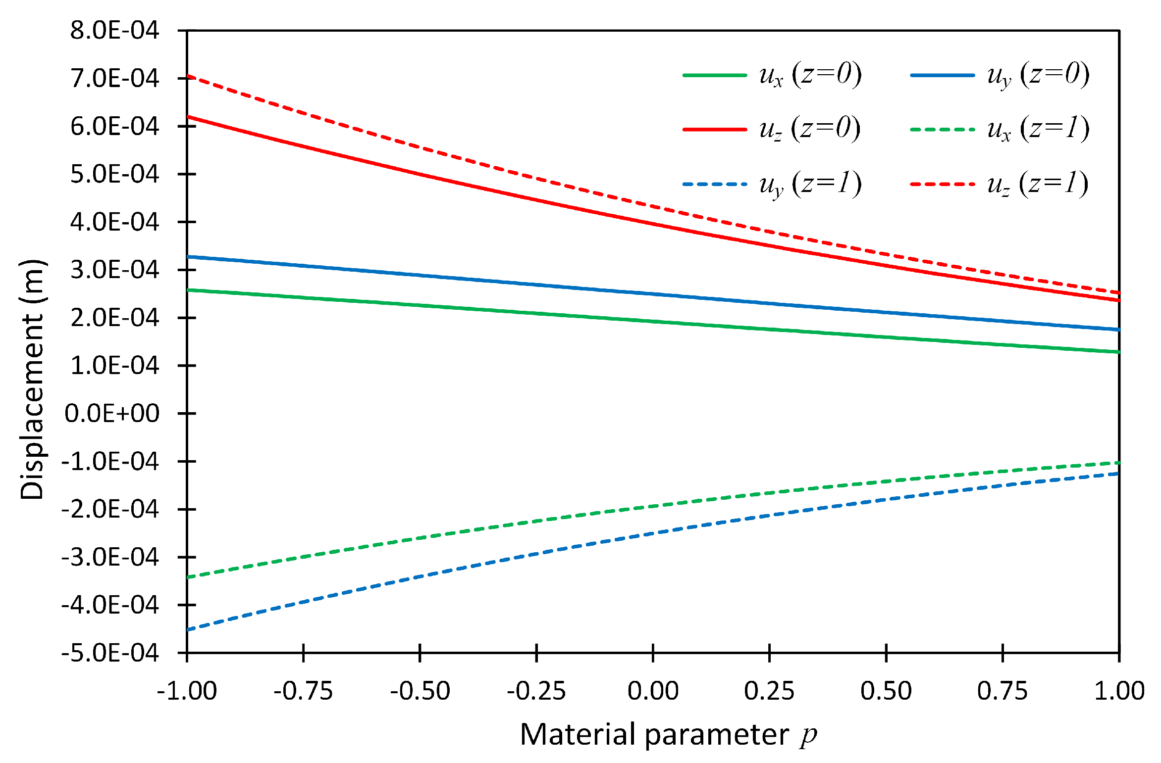
Figure 4.
The displacement components at two locations ()=() and () versus material parameter p for Example 1 considering boundary conditions CCCC.
Figure 4.
The displacement components at two locations ()=() and () versus material parameter p for Example 1 considering boundary conditions CCCC.
Figure 5.
The displacement components at two locations ()=() and () versus material parameter p for Example 1 considering boundary conditions CSFF.
Figure 5.
The displacement components at two locations ()=() and () versus material parameter p for Example 1 considering boundary conditions CSFF.
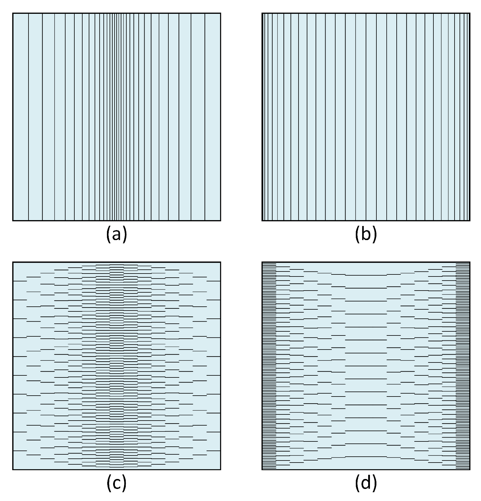
Figure 6.
Schematic representation of fiber orientations and volume fraction distributions for the FGM composite plate considered in Example 2; (a) , ; (b) , ; (c) , ; (d) , .
Figure 6.
Schematic representation of fiber orientations and volume fraction distributions for the FGM composite plate considered in Example 2; (a) , ; (b) , ; (c) , ; (d) , .
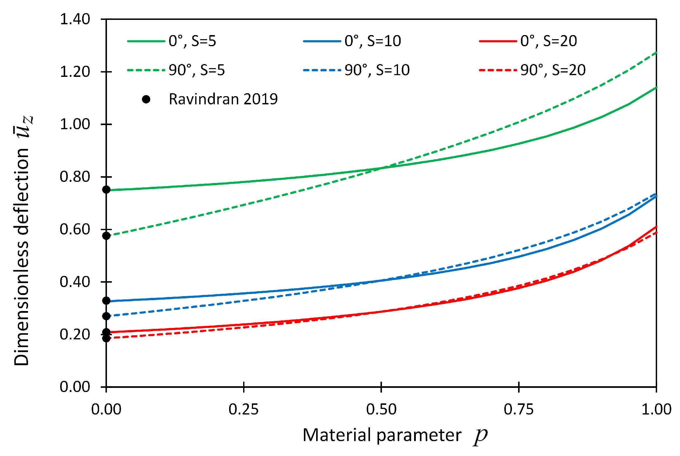
Figure 7.
The dimensionless displacement,
, at locations (
) = (
) versus material parameter
p for Example 2 considering boundary conditions SSSS; the reference solution given in (Ravindran 2019) [
19] is shown by solid dots.
Figure 7.
The dimensionless displacement,
, at locations (
) = (
) versus material parameter
p for Example 2 considering boundary conditions SSSS; the reference solution given in (Ravindran 2019) [
19] is shown by solid dots.
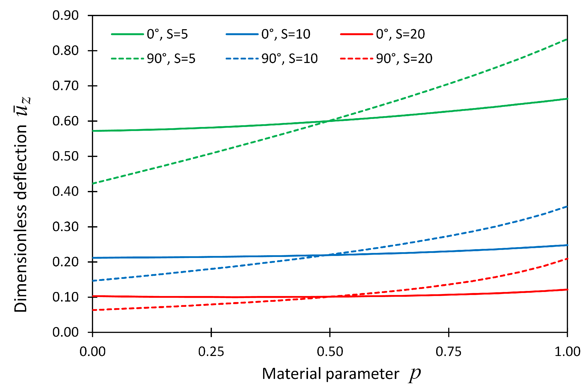
Figure 8.
The dimensionless displacement, , at locations () = () versus material parameter p for Example 2 considering boundary conditions CCCC.
Figure 8.
The dimensionless displacement, , at locations () = () versus material parameter p for Example 2 considering boundary conditions CCCC.
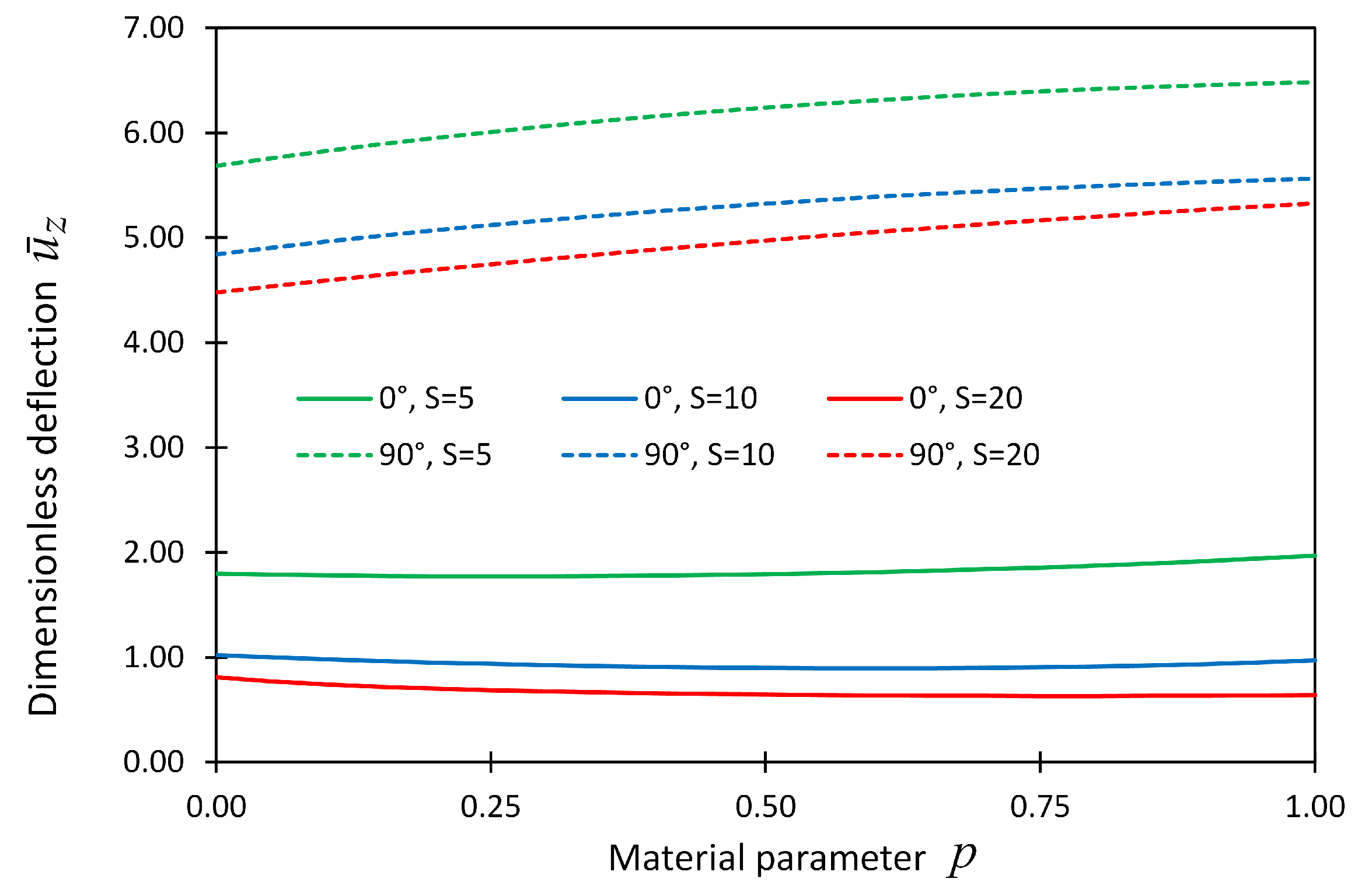
Figure 9.
The dimensionless displacement, , components at locations () = () versus material parameter p for Example 2 considering boundary conditions CSFF.
Figure 9.
The dimensionless displacement, , components at locations () = () versus material parameter p for Example 2 considering boundary conditions CSFF.
Figure 10.
Material parameters for Example 3.
Figure 10.
Material parameters for Example 3.
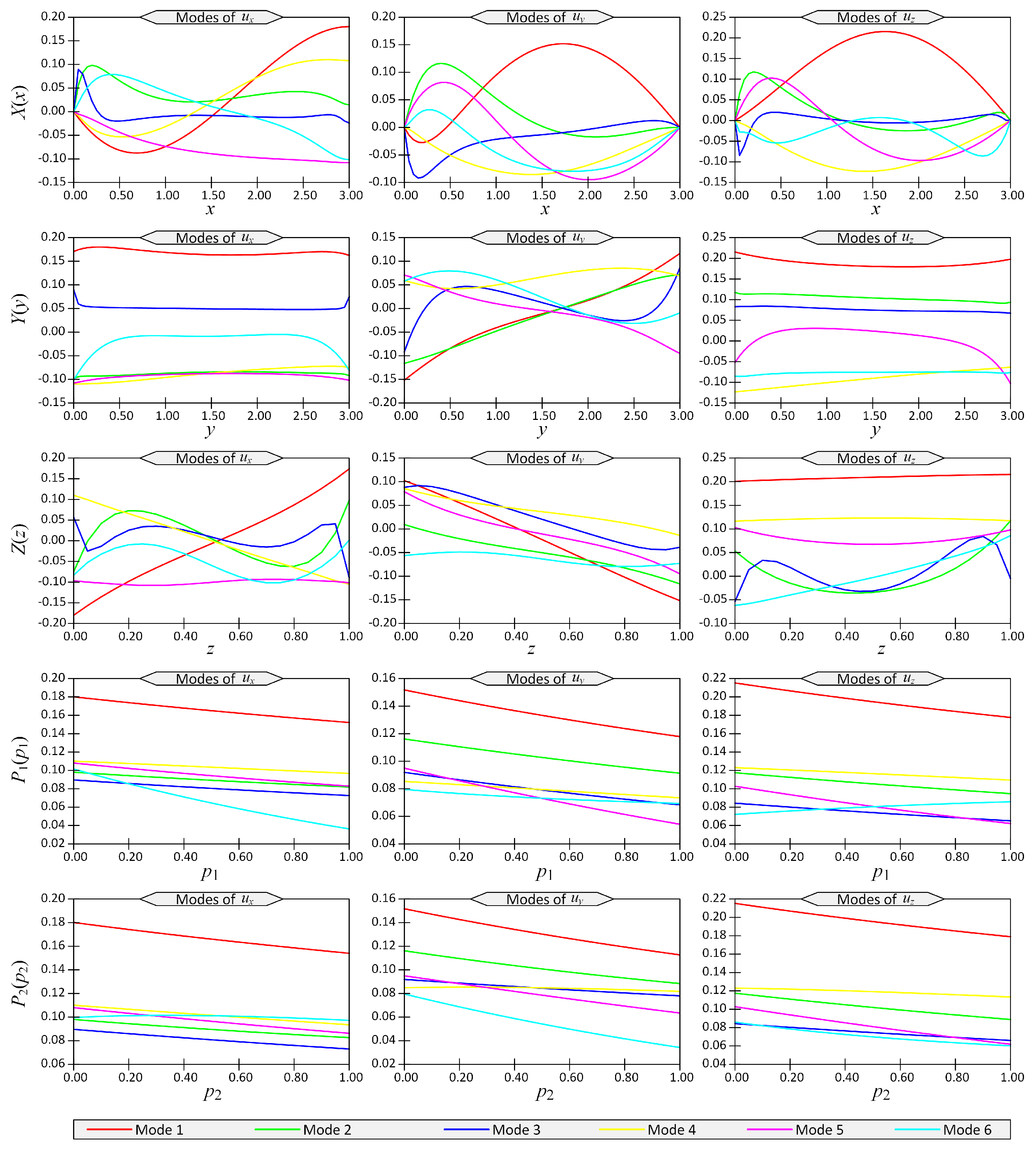
Figure 11.
The first six modes of displacement components () with respect to space coordinates () for Example 3.
Figure 11.
The first six modes of displacement components () with respect to space coordinates () for Example 3.
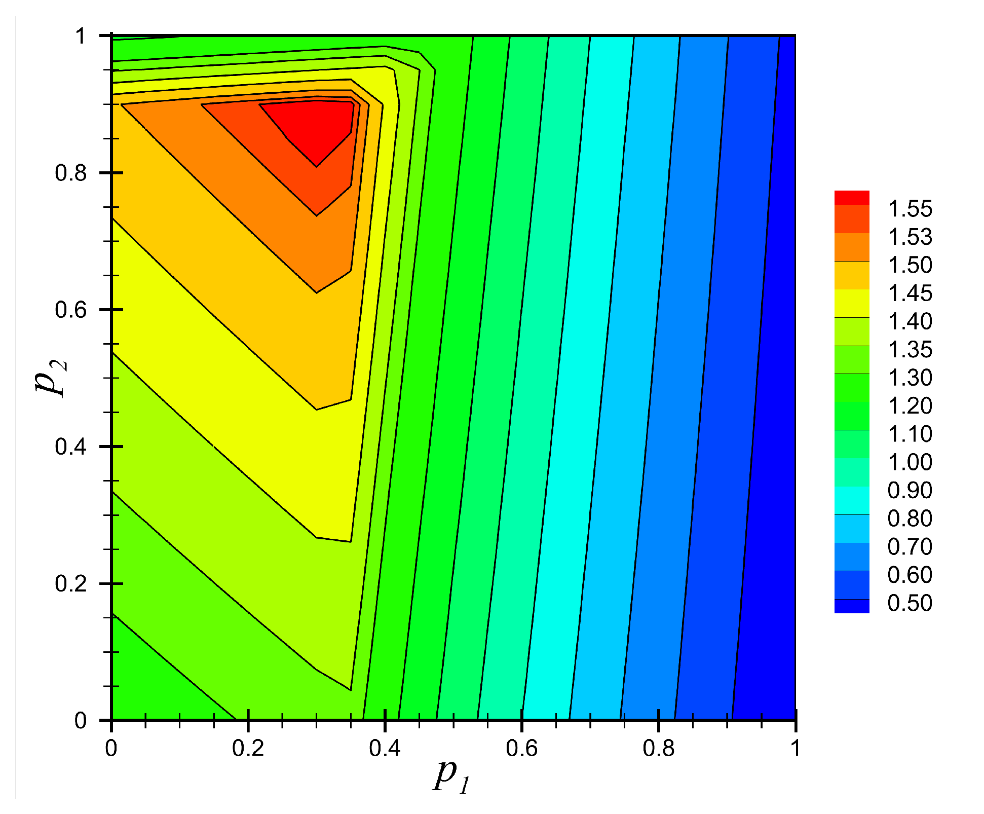
Figure 12.
Contour plot of the field of minimum factor of safety, , for the full range of material parameters and for Example 3.
Figure 12.
Contour plot of the field of minimum factor of safety, , for the full range of material parameters and for Example 3.
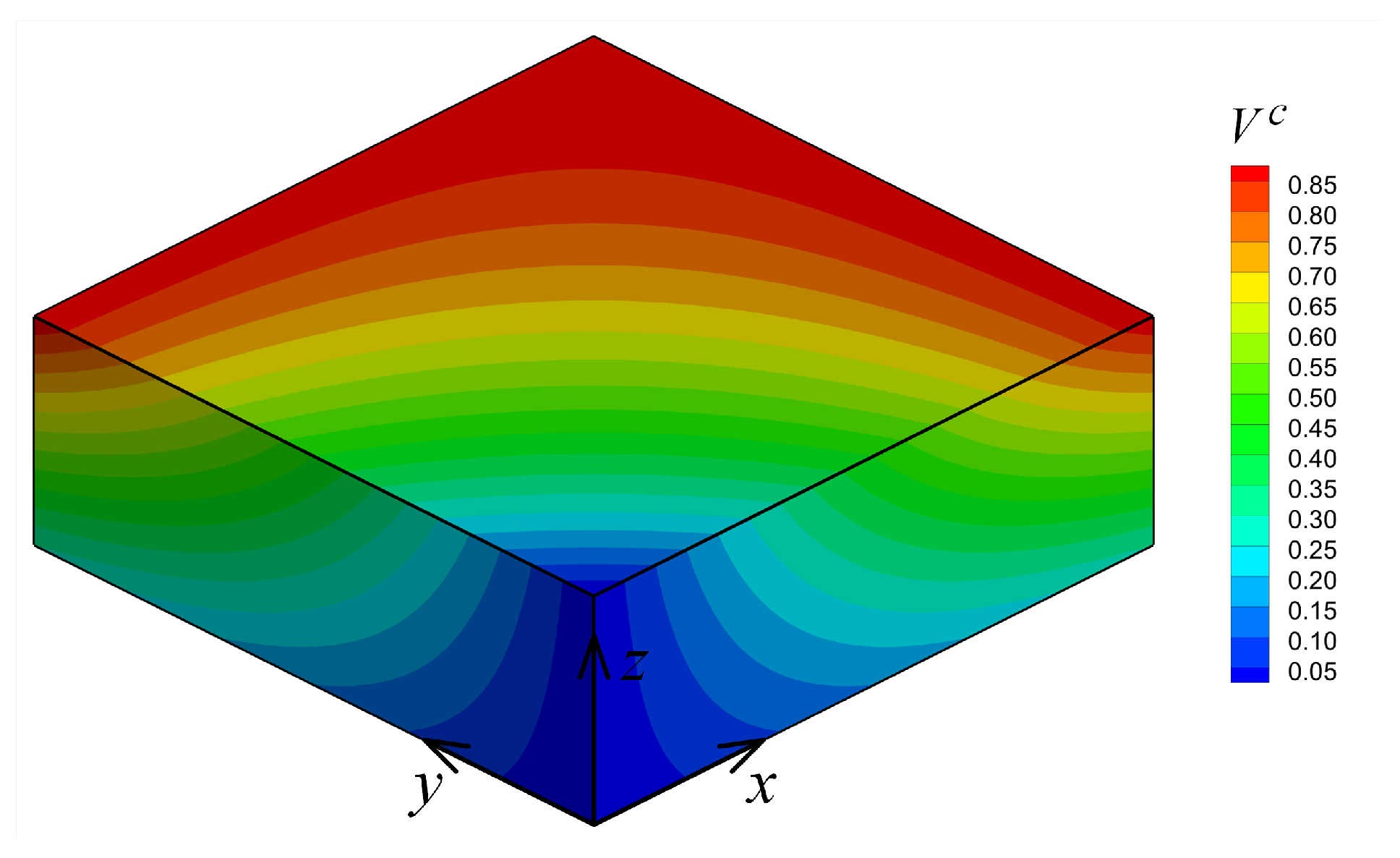
Figure 13.
Contour plot of volume fraction distribution for the optimum material parameters for Example 3.
Figure 13.
Contour plot of volume fraction distribution for the optimum material parameters for Example 3.
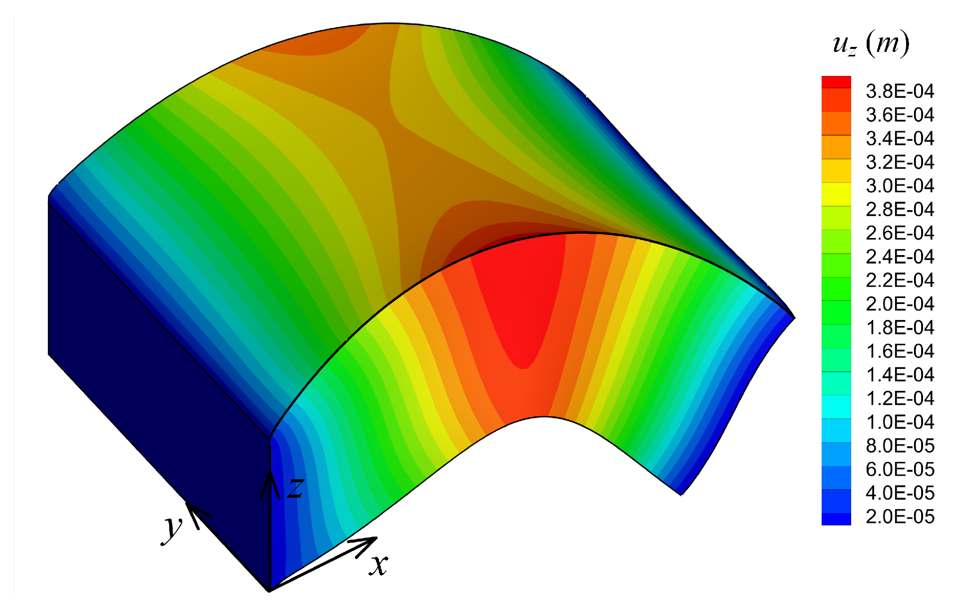
Figure 14.
Deformed configuration (not scaled) and contour plot of displacement for the optimum material parameters for Example 3.
Figure 14.
Deformed configuration (not scaled) and contour plot of displacement for the optimum material parameters for Example 3.
Table 1.
The indices sets
used in Equation (
7).
Table 1.
The indices sets
used in Equation (
7).
| Equation | Term | a | b | c | d | e | f |
|---|
| Equation (4) | 1 | x | x | x | y | 1 | 1 |
| 2 | x | x | y | y | 1 | 2 |
| 3 | x | x | z | z | 1 | 3 |
| 4 | x | y | y | x | 4 | 4 |
| 5 | x | y | x | y | 4 | 4 |
| 6 | x | z | x | z | 6 | 6 |
| 7 | x | z | z | x | 6 | 6 |
| Equation (5) | 1 | y | x | y | x | 4 | 4 |
| 2 | y | x | x | y | 4 | 4 |
| 3 | y | y | x | x | 1 | 2 |
| 4 | y | y | y | y | 2 | 2 |
| 5 | y | y | z | z | 2 | 3 |
| 6 | y | z | z | y | 5 | 5 |
| 7 | y | z | y | z | 5 | 5 |
| Equation (6) | 1 | z | x | x | z | 6 | 6 |
| 2 | z | x | z | x | 6 | 6 |
| 3 | z | y | z | y | 5 | 5 |
| 4 | z | y | y | z | 5 | 5 |
| 5 | z | z | x | x | 1 | 3 |
| 6 | z | z | y | y | 2 | 3 |
| 7 | z | z | z | z | 3 | 3 |
Table 2.
Explicit definition of plate boundary conditions regarding to Examples 1, 2 and 3.
Table 2.
Explicit definition of plate boundary conditions regarding to Examples 1, 2 and 3.
| B.C. Type | Face () | Face () | Face () | Face () |
|---|
| SSSS | | | | |
| CCCC | | | | |
| CSFF | | — | | — |
| CFSF | | | — | — |
Table 3.
Base engineering elastic constants for Example 1.
Table 3.
Base engineering elastic constants for Example 1.
| 6.89476 | GPa |
| 172.369 | GPa |
| 6.89476 | GPa |
| 3.44738 | GPa |
| 3.44738 | GPa |
| 1.37895 | GPa |
| 0.01 | |
| 0.25 | |
| 0.25 | |
Table 4.
The displacement components for three values of material parameter p, for Example 1, for boundary conditions SSSS obtained using different grid sizes.
Table 4.
The displacement components for three values of material parameter p, for Example 1, for boundary conditions SSSS obtained using different grid sizes.
| Dis. | Loc. | p | Ref. [24] | Present |
|---|
| {21 × 21 × 11 × 11} | {41 × 41 × 15 × 15} | {61 × 61 × 21 × 21} |
|---|
| z = 0 | −1 | 6.4876 | 6.3892 (1.5) | 6.4416 (0.7) | 6.4629 (0.4) |
| 0 | 4.5491 | 4.4825 (1.5) | 4.5182 (0.7) | 4.5324 (0.4) |
| 1 | 3.0359 | 2.9864 (1.6) | 3.0128 (0.8) | 3.0236 (0.4) |
| z = 1 | −1 | −7.0921 | −6.9544 (1.9) | −7.0267 (0.9) | −7.0577 (0.5) |
| 0 | −3.9492 | −3.8791 (1.8) | −3.9161 (0.8) | −3.9317 (0.4) |
| 1 | −2.0888 | −2.0502 (1.9) | −2.0705 (0.9) | −2.0792 (0.5) |
| z = 0 | −1 | 2.6853 | 2.5854 (3.7) | 2.6357 (1.8) | 2.6599 (0.9) |
| 0 | 1.7737 | 1.7070 (3.8) | 1.7406 (1.9) | 1.7568 (1.0) |
| 1 | 1.1232 | 1.0779 (4.0) | 1.1007 (2.0) | 1.1117 (1.0) |
| z = 1 | −1 | −3.643 | −3.4934 (4.1) | −3.5678 (2.1) | −3.6046 (1.1) |
| 0 | −2.0733 | −1.9945 (3.8) | −2.0338 (1.9) | −2.0531 (1.0) |
| 1 | −1.1419 | −1.0992 (3.7) | −1.1206 (1.9) | −1.1310 (1.0) |
| z = 0 | −1 | 21.134 | 20.823 (1.5) | 20.987 (0.7) | 21.055 (0.4) |
| 0 | 13.095 | 12.918 (1.4) | 13.012 (0.6) | 13.050 (0.3) |
| 1 | 7.7749 | 7.6602 (1.5) | 7.7207 (0.7) | 7.7457 (0.4) |
| z = 1 | −1 | 28.412 | 28.076 (1.2) | 28.249 (0.6) | 28.322 (0.3) |
| 0 | 16.568 | 16.384 (1.1) | 16.480 (0.5) | 16.519(0.3) |
| 1 | 9.4808 | 9.3593 (1.3) | 9.4229 (0.6) | 9.4492 (0.3) |
Table 5.
Engineering elastic constants of constitutive materials for Example 2.
Table 5.
Engineering elastic constants of constitutive materials for Example 2.
| Fiber | | 388 | GPa |
| 7.17 | GPa |
| 6.79 | GPa |
| 2.41 | GPa |
| 0.230 | |
| 0.486 | |
| Matrix | | 3.5 | GPa |
| 1.3 | GPa |
| 0.35 | |
Table 6.
The vertical dimensionless displacement, , for material parameter , for Example 2, for different thickness ratios, S, obtained using different grid sizes.
Table 6.
The vertical dimensionless displacement, , for material parameter , for Example 2, for different thickness ratios, S, obtained using different grid sizes.
| S | Ref. [19] | Present |
|---|
| {21 × 21 × 11 × 11} | {41 × 41 × 11 × 11} | {61 × 61 × 11 × 11} | {61 × 61 × 21 × 21} |
|---|
| 5 | 0.752 | 0.742 (1.3) | 0.746 (0.8) | 0.746 (0.7) | 0.750 (0.3) |
| 10 | 0.329 | 0.324 (1.5) | 0.327 (0.7) | 0.327 (0.6) | 0.328 (0.3) |
| 20 | 0.209 | 0.203 (2.7) | 0.207 (0.8) | 0.208 (0.5) | 0.208 (0.3) |
| 5 | 0.576 | 0.570 (1.0) | 0.572 (0.7) | 0.572 (0.7) | 0.575 (0.2) |
| 10 | 0.27 | 0.267 (0.9) | 0.269 (0.5) | 0.269 (0.4) | 0.270 (0.1) |
| 20 | 0.186 | 0.183 (1.6) | 0.185 (0.3) | 0.186 (0.1) | 0.186 (0.0) |
Table 7.
Engineering material constants for Example 3.
Table 7.
Engineering material constants for Example 3.
| Ceramic | | 348.43 | GPa |
| 0.24 | |
| 60 | MPa |
| 344.5 | MPa |
| Metal | | 201.04 | GPa |
| 0.3262 | |
| 215 | MPa |
| 215 | MPa |


