Value-at-Risk and Models of Dependence in the U.S. Federal Crop Insurance Program

Abstract

The federal crop insurance program covered more than 110 billion dollars in total liability in 2018. The program consists of policies across a wide range of crops, plans, and locations. Weather and other latent variables induce dependence among components of the portfolio. Computing value-at-risk (VaR) is important because the Standard Reinsurance Agreement (SRA) allows for a portion of the risk to be transferred to the federal government. Further, the international reinsurance industry is extensively involved in risk sharing arrangements with U.S. crop insurers. VaR is an important measure of the risk of an insurance portfolio. In this context, VaR is typically expressed in terms of probable maximum loss (PML) or as a return period, whereby a loss of certain magnitude is expected to return within a given period of time. Determining bounds on VaR is complicated by the non-homogeneous nature of crop insurance portfolios. We consider several different scenarios for the marginal distributions of losses and provide sharp bounds on VaR using a rearrangement algorithm. Our results are related to alternative measures of portfolio risks based on multivariate distribution functions and alternative copula specifications.

1. Introduction

The United States federal crop insurance program is one of the largest subsidized agricultural insurance programs in the world. Total liability exceeded 110 billion U.S. dollars in 2018 and resulted in roughly 6.5 billion U.S. dollars in indemnity payments (Risk Management Agency 2018). For major row crops, such as corn and soybeans, in excess of 80% of planted acres are insured under some variant of a federal crop insurance policy. A portion of the actuarially fair premium on the policies is subsidized by taxpayers; for policies with catastrophic coverage the subsidy can be 100 percent of premium but is closer to 60% of premium for the bulk of the policies sold through the program. As the most expensive mechanism for agricultural policy in the United States, any actuarial changes to the program can have major impacts on government expenditures, insurance uptake, and production decisions.

Policies are priced by the Risk Management Agency (RMA) of the U.S. Department of Agriculture (USDA) but are serviced by approved private insurers. These insurers are subject to the Standard Reinsurance Agreement (SRA) which controls several aspects of their relationship with the federal government. The SRA allows private insurers to cede the riskiest portions of their portfolios to a government-backed reinsurance fund. Insurers can generate economic rents if they have a method of pricing that is more accurate than that used by the RMA; they can strategically cede or retain policies (Ker and McGowan 2000). They have an advantage in being able to observe prices from the RMA before choosing which policies to cede. Remaining risk is transferred to international reinsurers who engage in substantial business with the approved insurance providers.

Because of significant government involvement in the program, and following demand from reinsurers, quantifying the risk associated with the entire crop insurance portfolio is an important and challenging problem. Unlike other lines of insurance, losses across members of the insurer’s portfolio cannot be considered independent. Latent variables induce dependence by affecting crop production across a number of locations. The most obvious of these latent variables is weather. But many other factors that affect crop production, such as pests, disease, and management practices, are spatially correlated. Positive spatial dependence in crop production has been forwarded as an explanation for the lack of development of private crop insurance markets. However, Holly Wang and Zhang (2003) showed that spatial dependence dissipates at a sufficient speed such that private insurance markets should be feasible. Government involvement may actually crowd out private insurance.

We estimate value-at-risk (VaR) for a hypothetical portfolio of crop insurance policies. The marginal distributions determining the aggregate loss are allowed to follow an arbitrary distribution leading to an inhomogeneous portfolio from the insurer’s perspective. Dependence relationships between individual losses are unknown. As any joint distribution can be decomposed into marginal distributions and a copula function, one implication is that the form of the copula is also unknown. In spite of the lack of knowledge about the appropriate copula, reliable bounds on VaR can be computed using the rearrangement algorithm of Embrechts et al. (2013). We calculate the VaR using the rerrangement algorithm and a variety of copula specifications.

The problem of reliable estimates for VaR extends beyond private insurers to reinsurers. Reinsurers handle risks from more than one insurer so the portfolio of the international reinsurer consists of risks from a diverse group of entities. Most crop insurers operate in a geographically concentrated area leading to greater dependence in their portfolios. To develop an aggregate loss distribution for their holdings, the reinsurer is then tasked with pooling loss distributions for the underlying insurers. This can be challenging for reinsurers handling crop insurance portfolios because of difficulties in separating systemic and pool-able losses (Odening and Shen 2014).

Although the federal government can handle any reinsurance losses through the program, budgeting decisions with respect to the crop insurance program take into account the probability of worst-case losses (Hayes et al. 2003). The probability of a large portfolio loss is important for predicting variability in future government outlays. Likewise, insurers and reinsurers engage in loss reserving. Loss reserving models produce an estimated total loss reserve as the required loss reserve (the amount needed to meet all indemnifications) is not known until after indemnities are paid out. The issue of calculating adequate reserves is similar for financial institutions dealing with operational risk. Insurers, reinsurers, and financial institutions often base reserving decisions on VaR calculations; in the insurance industry, VaR is typically termed probable maximum loss (PML).

By calculating VaR under several different dependence models and deriving sharp bounds using the rearrangement algorithm, we also provide estimates of model risk in crop insurance applications. As the marginal distributions are the same in any case, the model risk we describe is specifically related to the dependence model. In line with previous findings by Goodwin and Hungerford (2014), there is a substantial amount of model risk induced by the choice of the dependence structure. Therefore, any top-down approach to loss aggregation should take into account the model risk from dependence in reserving decisions. Because the crop insurance program is publicly funded, the amount of overall risk (of which model risk is one part) in the program causes difficulties in accurately projecting public expenditures.

The general approach we take is to assume marginal distributions and merge them into a joint distribution using a copula function. This approach is referred to by Aas and Puccetti (2014) as top-down aggregation. An alternative approach is bottom-up aggregation where drivers of risk types are identified and a model is developed for the risk factors. Simulations can then be used to aggregate risk over a number of different scenarios for the evolution of the risk factors. Bottom-up aggregation is also frequently used by crop insurance modelers. Because the fundamental driver of yield risk is weather, catastrophe modelers often model the evolution of weather, simulate a number of scenarios, and then translate these weather scenarios into yield losses. In either case, using top-down or bottom-up approaches for risk aggregation, the end result is construction of a measure of portfolio risk from marginal risk information.

2. Crop Insurance Policies and Actuarial Methods

The U.S. federal crop insurance program encompasses a wide range of different policy types, crops, and locations. The most widely purchased policies are yield and revenue insurance policies. These may be purchased at the farm or county level. In the latter case, the loss is determined by the average yield or revenue in the county. Farm level policies are priced using production data from an individual farm. Whether at the farm or county level, the actuarial methods underlying pricing are similar. A number of adjustments are made in pricing farm level policies because these policies usually have a much shorter time series of available data.

Revenue is the product of quantity and price. Quantity is usually given by crop yield: the amount of crop production per unit of land. The loss on revenue and yield insurance policies are determined by prices and yields. To generate the probabilities of loss required to price crop insurance policies, we have the option of modeling losses themselves or directly modeling prices and yields. Up to harvest, yields for the coming year can be considered random variables. Randomness results from the stochastic nature of crop production as affected by weather, pests, and other uncertainties. Both yield and revenue insurance are multiple peril and indemnify losses from a number of different sources of risk.

For yield insurance policies, the loss on the policy is given by

$${\mathrm{loss}}_{\mathrm{yield}}=max(0,(\lambda \overline{y}-y)p),$$

(1)

where $\overline{y}$ is the historical mean yield or expected yield, y is the realized yield, $\lambda \in (0,1)$ is the coverage level, and p is a deterministic price. The only stochastic element in Equation (1) is y. Under a revenue insurance policy,

$${\mathrm{loss}}_{\mathrm{revenue}}=max(0,(\lambda \overline{y}{p}_p-y{p}_h)),$$

(2)

where the variables are similarly defined. In this case, $p_P$ is a projected or planting-time price and $p_h$ is the realized or harvest-time price for the crop. Only the yield y and realized price $p_h$ are stochastic. Some revenue insurance policies extend the guaranteed revenue in Equation (2) from $\lambda \overline{y}{p}_p$ to $\lambda \overline{y}max(p_p,p_h)$ to provide additional price coverage.

Both Equations (1) and (2) reveal several interesting aspects of these policies. First, they require a model for the evolution of crop yields. Second, revenue insurance policies also require a model of dependence between the stochastic yield and price. The random variables in the loss equations are likely to be correlated across space. Lastly, because policies in the same county are written at different coverage levels, losses on different policies are also correlated within the same county. Given the complexities in pricing a single policy, determining risk in a portfolio of crop insurance policies is a complicated task.

The actuarial process of pricing individual policies in the federal program has received considerable attention because of the close link between actuarial practices and program losses. The RMA also has a legislative mandate to produce premium rates that are actuarially fair. Early work focused on estimation of the marginal distribution of crop yields and if a best distribution could be found. Applications included parametric distributions (Gallagher 1986; Ozaki and Silva 2009; Sherrick et al. 2004), nonparametric distributions (Goodwin and Ker 1998), and semiparametric distributions (Ker and Coble 2003; Tolhurst and Ker 2014). Although no clear winner has emerged, the tendency has been to gravitate toward the use of flexible parametric distributions that can accommodate skewness and excess kurtosis. Non-parametric approaches are used when large samples are available. Current rating methods employed by the RMA use truncated normal distributions.

In most cases, the distributions are not fitted to observed yields but to normalized yields. Since 1940, average corn yields in the United States have increased roughly 8 times. Better management practices and plant breeding have enabled remarkable growth in the mean of the yield distribution. To account for technological change, observed yields are detrended and probability distributions are estimated on deviations from trend. The detrending procedure has varied but researchers have used robust regression, locally weighted scatterplot smoothing, and deterministic models. Several authors have considered joint estimation of the trend and density using time-varying distributions (Tolhurst and Ker 2014; Zhu et al. 2011).

Revenue insurance is now the most popular form of insurance in the crop insurance program and accounts for over 80% of total liability. The increasing prevalence of revenue insurance has prompted research into dependence between prices and yields. Goodwin and Hungerford (2014) and Hungerford and Goodwin (2014) examined yield-price dependence as it affects systemic risk. One problem with pricing revenue insurance policies is that the samples used to identify the copula, or more specifically dependence between prices and yield, are small in practice. The issue was further considered by Ramsey et al. (2019) who found that, although there was little support for the assumption of a Gaussian copula, the economic impact of choice of copula on pricing for individual policies was minor. Rates were affected more by changes in the marginal distributions.

Because yield risks are spatially correlated, several authors have also examined the measurement of dependence between yields across space. This is important not only for measuring systemic risk but also for informing estimates in locations with little available yield information. If the dependence structure is known, then data from a number of locations can be pooled to arrive at more accurate estimates for individual policies. Okhrin et al. (2013a) examined the diversification effects of weather indices that can be used in lieu of yield and revenue insurance. Porth et al. (2016) discussed an approach for improved pooling of systemic weather risk using simulated annealing. Ker et al. (2015) and Park et al. (2018) developed methods to average or smooth yield distributions across locations and achieve more accurate rates.

While dependence in losses across space has attracted significant attention, there are also dependencies among policies sold at the same location. Because of the way area policies are structured, a policy purchased at the 90% coverage level will always pay out when a policy purchased at the 70% coverage level is indemnified. However, the converse is not true. These dependencies do not present a major practical problem because the majority of policies are sold at the farm level and are usually at the highest coverage levels. However, if we wished to directly model a portfolio of policies across counties and coverage levels, intra-county dependence in the portfolio would also need to be taken into account.

Previous work on the modeling of crop yields is germane to measurement of portfolio risk because one can either model the losses directly or derive the losses from a model of yields. As an example, to determine a loss from the mean, one needs a model or procedure for determining the mean of the distribution. The same factors that generate dependence between yields at different locations cause systemic risk for the crop insurance portfolio. In modeling either losses, loss costs, or yields, several assumptions have to be made on the evolution of the random variables and the stability of the distributions generating the random variables. Unfortunately, there is no single objective criteria for determining which approach is best.

3. Dependence and Portfolio Risk

In many applications, the starting point for assessing the aggregate risk inherent in an insurance portfolio is the value-at-risk (VaR). The aggregate loss S for the portfolio is a function of its individual factor losses $x_i$ so that

$$S=\sum _{i=1}^K{x}_i,$$

(3)

for a portfolio comprised of K factors. The VaR for the portfolio is

$$Va{R}_{\alpha }\left(S\right)=F^{-1}(S;\alpha )=\inf (S\in R:F\left(S\right)>\alpha ),$$

(4)

with confidence level $\alpha$ where $F(·)$ is the distribution function of the aggregate loss S. VaR is usually intended to capture the risk of extremely large losses and $\alpha$ takes values in the range of 0.9 to 0.99. For a given portfolio and time horizon, the probability of a loss larger than the VaR is at most $\alpha$.

To calculate the VaR, we require the distribution function of the aggregate loss or a model for the joint distribution of the factors in the portfolio. There are a number of choices for the model of the joint distribution but some models impose strict assumptions on the behavior of the underlying variables. For instance, the assumption of a Gaussian joint distribution implies that the marginal behavior of the variables is Gaussian. An appealing method for constructing the joint distribution is the use of copulas which allows the analyst to split the problem into choice of the marginals and a dependence structure. The dependence structure is modeled by the copula function.

The copula is a function in K dimensions that allows a joint distribution function to be given by

$$F(x_1,\cdots ,x_K)=C(F_1\left(x_1\right),\cdots ,F_K\left(x_K\right)),$$

(5)

where $F_i(·)$ is the marginal distribution function of random variable $x_i$. At least for continuous marginal distributions, the copula C is unique and contains all dependence information in the joint distribution. This result, originally discovered by Sklar (1959), is both powerful and practically useful. As indicated in the preceding section, there are a number of situations where the marginal distributions of the variables have been thoroughly investigated or can be motivated by a reasonable appeal to economic or statistical theory. Less is known about the dependence structure between variables and the copula formulation allows the analyst to concentrate on addressing this unknown dependence.

There are two important copulas known as the Fréchet upper and lower bounds. For a given copula $C(u_1,\cdots ,u_K)$

$$max\left(\sum _{i=1}^K{u}_i-K=1,0\right)\le C(u_1,\cdots ,u_K)\le min(u_1,\cdots ,u_K),$$

(6)

for all $C(·)$ and $u_1,\cdots ,u_K\in [0,1]$. The copula on the left is the Fréchet lower bound and the copula on the right is the Fréchet upper bound. The upper bound is known as the comonotonic copula because it denotes perfect positive dependence between the random variables. The lower bound is countermonotonic and represents perfect negative dependence, but is only a well-defined copula in two dimensions. All copulas capture dependence structures somewhere between perfect positive and perfect negative dependence, and therefore they must be within the Fréchet bounds.

The likelihood function for the copula is

$$L=\sum _{j=1}^{N}logC(F_1\left(x_{j1}\right),\cdots ,F_d\left(x_{jK}\right))+\sum _{i=1}^K\sum _{j=1}^{N}log{f}_i\left(x_{ji}\right),$$

(7)

with two terms that capture the dependence structure’s effect on the likelihood and the contribution of the univariate marginal distributions respectively. The most common approach to obtaining the joint distribution is to use a procedure known as Inference from Margins whereby the parameters of the marginal distributions are first obtained and then the copula part of the likelihood is maximized taking the marginal parameters as given. In many cases, the parameter of the copula has a one-to-one relationship with measures of dependence such as Kendall’s tau or Spearman’s rho. It is not necessary to maximize the pseudo-likelihood. An estimate of the copula parameter can be obtained by first estimating the dependence measure and transforming the empirical measure to the copula parameter via calibration. Unfortunately, for some copulas (such as the t) there is no direct relationship between common dependence measures and some of the copula parameters.

Important features of copulas are their tail dependence properties. These properties can have large impacts on VaR estimates because VaR is usually concerned with the tail of the loss distribution. Two coefficients

$${\lambda }_U=\underset{u\to 1}{lim}Pr(U_1\ge u|U_2\ge u)=\underset{u\to 1}{lim}\frac{1-2u+C(u,u)}{1-u},$$

(8)

$${\lambda }_L=\underset{u\to 0}{lim}Pr(U_1\le u|U_2\le u)=\underset{u\to 0}{lim}\frac{C(u,u)}{u}$$

(9)

define the upper and lower tail dependence coefficients respectively. Tail dependence is realized whenever one of the coefficients is positive. Among the most popular bivariate copulas, the Gaussian copula has no tail dependence, the t copula has tail dependence in both tails, the Clayton copula has tail dependence in the lower tail, and the Gumbel copula has tail dependence in the upper tail. Both the Gumbel and Clayton copulas can capture asymmetries in tail dependence and have been used in many applications where dependence between the elements of a portfolio is expected to be stronger in the case of major portfolio losses.

While the Archimedean copulas (Gumbel and Clayton) can capture dependence asymmetry, their use in multivariate applications is questionable. They usually are controlled by a single parameter even in many dimensions. For instance, whereas a four-dimensional Gaussian copula describes dependence with essentially six parameters, a four-dimensional Gumbel copula has only a single parameter. Because of this limitation on multivariate Archimedean copulas, several authors have proposed pair-copula constructions that “stack” bivariate copulas and result in more complicated dependence relationships while maintaining parsimony. The most popular methods are hierarchical Archimedean copulas and vine copulas (Nikoloulopoulos et al. 2012; Okhrin et al. 2013b).

Copulas have been used to examine dependence relationships in a number of settings. Yang et al. (2015) considered dependence between international stock markets. In an insurance application, Tamakoshi and Hamori (2014) measured dependence between the credit default swap indices of insurers. Patton (2009) provide a number of examples and applications of copulas to financial time series. Some implications and use of copulas in credibility ratemaking for auto insurance are provided in Frees and Wang (2006). A common theme in all of these works is that the copula model used can have a major impact on portfolio losses and risk—whether in a financial or insurance setting. Unfortunately, there are few methods of choosing the ideal form of the copula. The analyst is usually left with selecting a copula model from a set of possible models that may or may not include the true model.

Because of the relationship shown in Equation (5), it is relatively straightforward to compute the VaR if presented with marginal distributions and the copula function. If the marginals and copula are not known, they can be estimated from the data. Perhaps the easiest approach is to simulate uniform random variables with a given dependence structure by drawing from the estimated copula. The uniform draws are then passed through the marginal inverse cumulative distribution functions producing a simulated dataset from the joint distribution of K random variables. For each iteration of the simulation, the total portfolio loss is calculated. The $\alpha$ VaR is the $\alpha$ empirical quantile of the simulated distribution of portfolio losses.

Embrechts et al. (2013) contains a detailed discussion on the use of VaR in operational risk settings and many of the concepts are immediately applicable in insurance settings. Following Embrechts et al. (2013), define the upper and lower bounds for the VaR of the portfolio as

$${\overline{VaR}}_{\alpha }\left(S\right)=\sup (Va{R}_{\alpha }\left(S\right):F_i\in \gamma (F_1,\cdots ,F_K))$$

(10)

$${\underline{VaR}}_{\alpha }\left(S\right)=\inf (Va{R}_{\alpha }\left(S\right):F_i\in \gamma (F_1,\cdots ,F_K)),$$

(11)

where $\gamma (F_1,\cdots ,F_K)$ is the Fréchet class of all possible joint distributions for the portfolio having the given marginal distributions. These can be restated in terms of the copula as

$${\overline{VaR}}_{\alpha }\left(S\right)=\sup (Va{R}_{\alpha }\left(S\right):C\in {ϵ}_K))$$

(12)

$${\underline{VaR}}_{\alpha }\left(S\right)=\inf (Va{R}_{\alpha }\left(S\right):C\in {ϵ}_K),$$

(13)

where ${ϵ}_K$ is the set of all copulas of dimension K. Embrechts et al. (2013) define ${\overline{VaR}}_{\alpha }$ and ${\underline{VaR}}_{\alpha }$ as the worst and best case VaR respectively. Moreover, the bounds given in Equations (10) and (11) cannot be improved without additional information on the dependence structure. The difference between the bounds is the difference in risk that arises from the dependence structure (i.e., copula) and is defined by Aas and Puccetti (2014) as the dependence uncertainty spread.

In general, the VaR for the portfolio is not the sum of VaR for the marginal risk factors. One exception is the case of comonotonic dependence. Comonotonic dependence is a relatively conservative assumption as it implies perfect dependence between the factors. The copula for factors with comonotonic dependence must be the upper Fréchet bound. Interestingly, there are cases where independence results in a worse (larger) VaR restimate than under comonotonicity (Mainik and Embrechts 2013). The point stressed by Embrechts et al. (2013) is that the comonotonic copula is not typically the solution for Equation (10). Likewise the countermonotonic copula is not generally a solution to Equation (11).

Because the comonotonic and countermonotonic copulas do not generally produce the best and worst case VaR, Embrechts et al. (2013) develop a reordering algorithm to compute sharp bounds on VaR under best and worst case dependence scenarios. Determining the bounds is also developed in Puccetti and Rüschendorf (2012) and Puccetti (2013). As explained in Aas and Puccetti (2014), the rearrangement algorithm is relatively simple and consists of rearranging each column of a matrix until they are oppositely ordered to the sum of the other columns. The algorithm terminates in a finite number of steps and the termination condition depends on whether one is calculating ${\overline{VaR}}_{\alpha }$ or ${\underline{VaR}}_{\alpha }$. Several empirical applications have shown the rearrangement algorithm to generate reasonable VaR estimates conditional on the underlying marginal distributions.

The algorithm can be applied to portfolios of high dimension where the estimation and validation of a given dependence structure can be difficult. It is easy to estimate a Gaussian copula using calibration methods. But in high dimensions, multiple parameter copulas such as the t can cause estimation problems. Optimization is required over a large parameter space. Moreover, the best fitting copula is usually selected according to a fit criteria such as the Akaike information criterion (AIC). There is no guarantee that the set of copulas being considered will include any copula with adequate fit. While the copula paradigm provides a useful approach for constructing a joint distribution and measuring associated portfolio risk, it does not necessarily provide adequate information on dependence uncertainty and model risk. The problem is made even more difficult in cases of limited data where estimation of the copula may be impossible.

Aas and Puccetti (2014) present an interesting application of the rearrangement algorithm to capital requirements for Norway’s largest bank: DNB. They also discuss some of the challenges in applying the algorithm in a real situation. In their case, some of the risk factors have limited data and the dependence structure used by the bank is formed on the basis of expert opinion. Fitting several types of copulas and using the rearrangement algorithm, Aas and Puccetti (2014) show that dependence uncertainty can be quite large in practical applications and that VaR can vary significantly based on the type of copula used to capture the dependence structure. Adding more information on dependence among groups of the random variables results in considerably tighter bounds on the VaR.

The VaR is a single measure of the risk of the portfolio and subject to several criticisms. In particular, the VaR is almost always estimated from historical information. To estimate probabilities from historical events, it is necessary to make an assumption that the events are independent and identically distributed. This is rarely the case in practice, especially when dealing with crop yields or revenue. Crop insurers are also routinely confronted by small sample sizes that place practical constraints on the set of admissible models. These difficulties feed over into calculations of dependence and portfolio risk as noted by both Hungerford and Goodwin (2014) and Ramsey et al. (2019).

Many of the problems of estimating a measure of portfolio risk in crop insurance are analogous to problems in the operational risk space (Cope et al. 2009). Estimation of the loss distribution can be highly sensitive to large losses occurring with low frequency. Data is scarce enough that appeals to extreme value theory for the distribution of losses cannot be justified. Very little is known about the dependence process except that losses are correlated across space. This makes the modeling of portfolio risk in crop insurance a challenging problem. The empirical applications that follow present two possible approaches for addressing these concerns and arriving at a measure of portfolio risk.

4. Empirical Applications

We considered two empirical applications aimed at measuring risk in a portfolio of crop insurance policies. The first estimated VaR for a portfolio of corn yield insurance policies in Illinois. The loss in this case was the normalized yield deviation from trend. In other words, we directly modeled the crop yield in each county and constructed losses in terms of a normalized yield. VaR was calculated using data on these yield losses. The second application is more general; we modeled the loss cost ratio for corn policies in a single crop reporting district in Iowa. The loss cost modeling is easily generalized to other crops and locations. It also avoids some of the intricacies in direct modeling of yields. However, there was less data to work with and the loss cost distribution was assumed to be stable across the time period.

4.1. VaR for a Portfolio of Yield Policies

We obtained all-practice corn yields in Illinois at the county level for 102 counties from 1955 to 2015. Because yields change over time with advances in production technology and management practices, the marginal distribution of yields must be normalized. Each observed yield was thought of as being drawn from a unique distribution at each location and in each year (Tack and Ubilava 2013). The distribution of interest from the insurer’s perspective was the projected yield distribution for the upcoming year. Therefore, this application considers a purely synthetic portfolio of policies that realize a loss anytime the yield is below its mean. Using Equation (1), the coverage level was 100% of the expected average yield.1 This approach could be used to capture portfolio dependence among a suite of different policies so long as we are willing to model dependence between policies at different coverage levels.

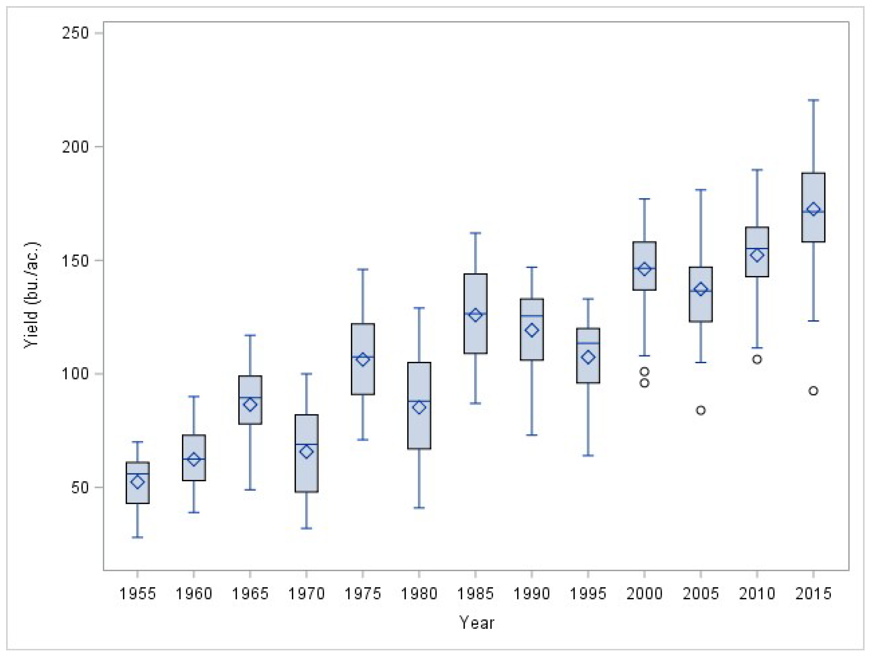
Because the distribution of yields changes over time, we first fit a trend to the yields in each county using locally weighted scatterplot smoothing (Cleveland and Devlin 1988). The smoothing parameter was selected automatically using a corrected version of AIC suggested in Hurvich et al. (1998). The residuals from trend were then recentered about the last year in the series. Figure 1 shows boxplots of yields from all Illinois counties at five year intervals. We can see that there was significant variation in yields across space and time. Mean and median yields have consistently risen and the standard deviation of the distribution also appears to have increased.

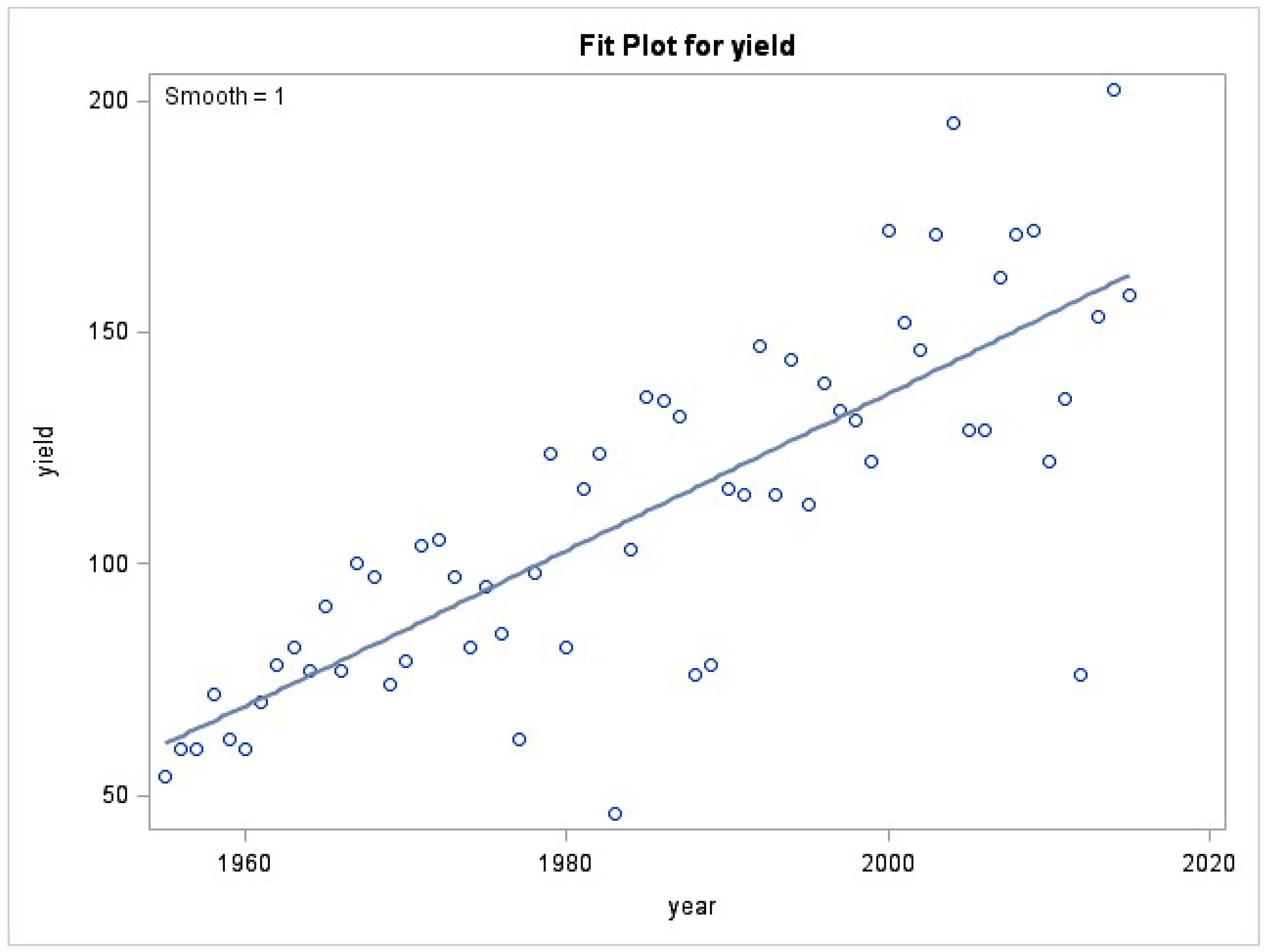
Figure 2 shows yields in Adams County, Illinois along with the fitted locally weighted scatterplot smoothing (LOESS) line. In this case, the trend appears nearly linear. Large losses have occurred over the 50 year period; a notable loss was during the drought conditions that characterized crop production throughout the midwest in 2012. There is also visual suggestion of heteroskedasticity, justifying the recentering procedures. Using the normalized yields, we then constructed losses from the projected mean yield in each year. These losses were used to fit the marginal distributions and copula functions.

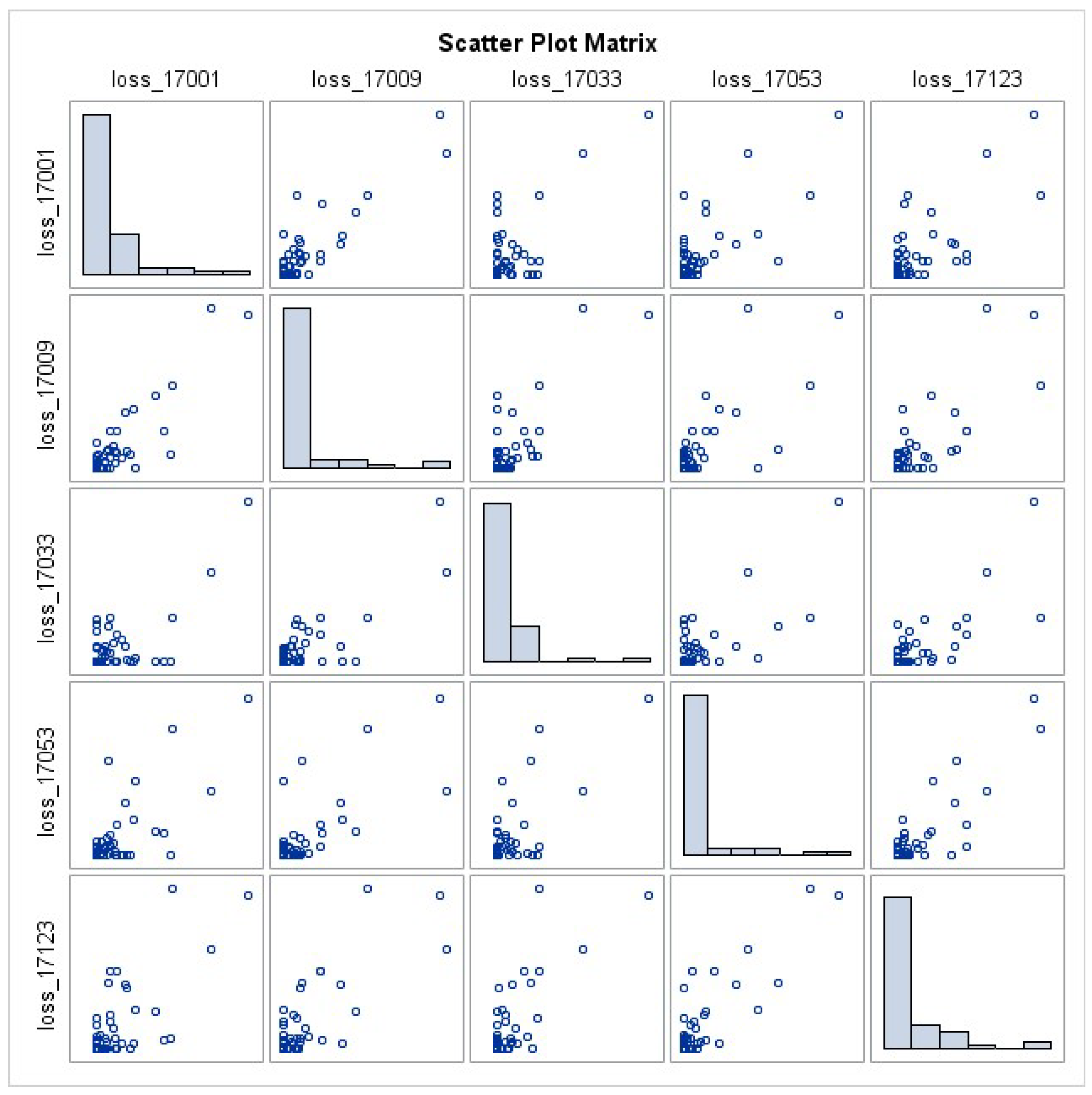
Scatterplots of yield losses across five randomly selected Illinois counties are shown in Figure 3. Given the close geographic proximity of the counties, it should be no surprise that there was a high degree of correlation across space. There were a number of years where losses are observed in one county but not another; the important point is that these losses tend to be relatively small. The largest loss in almost all of the counties is observed in a single year: 2012. Pearson correlation coefficients across the same five counties are shown in

Table 1. Pearson correlation of losses across five counties.

County FIPS	Pearson Correlation Coefficients
	17001	17009	17033	17053	17123
17001	1	0.88652	0.70929	0.74421	0.73467
17009	0.88652	1	0.80876	0.74871	0.80017
17033	0.70929	0.80876	1	0.7359	0.77594
17053	0.74421	0.74871	0.7359	1	0.86371
17123	0.73467	0.80017	0.77594	0.86371	1

. There is high correlation although this should not be considered representative of all counties across the state. It does, however, suggest that dependence across counties could be an important element determining portfolio losses.

The aggregate loss for the portfolio of policies is given by

$$S=x_{17001}+\cdots +x_{17203},$$

(14)

and is simply the sum of the losses in the 102 counties of Illinois. The risk factors $x_i$ are indexed by their Federal Information Processing Standards (FIPS) code at the county level. We consider several parametric distributions for the losses including the exponential, gamma, inverse Gaussian, lognormal, and Weibull distributions. These distributions can take a wide range of shapes, offer substantial flexibility, and have non-negative support. Goodness of fit was determined using the Cramer von Mises (CvM) statistic which compares the estimated loss distribution to the empirical cumulative distribution function. The CvM statistic is defined as

$$\mathrm{CvM}=N{\int }_{-\infty }^{\infty }{(F_n\left(x\right)-F\left(x\right))}^{2}dF\left(x\right),$$

(15)

where $F(·)$ is the estimated cumulative distribution function and $F_n(·)$ is the empirical cumulative distribution function. The selected marginal distributions and parameter values for the first ten counties are shown in

Table 2. Marginal loss distributions and parameter values for 10 counties in Illinois (IL).

County FIPS	Model	Theta	Alpha/Xi
17001	Exponential	8.32
17003	Exponential	6.63
17005	Exponential	8.45
17007	Gamma	158.42	0.04
17009	Inverse Gaussian	14.29	0.12
17011	Gamma	149.04	0.04
17013	Gamma	133.91	0.04
17015	Gamma	185.26	0.04
17017	Inverse Gaussian	13.79	0.08
17019	Gamma	172.67	0.04

. For the majority of counties, the gamma distribution was best fitting (76), followed by the exponential (17), and inverse Gaussian (9). Because the distribution varies across counties, the portfolio is inhomogeneous.

Given the selected parametric marginal distributions, we calculated the VaR for the portfolio under different assumptions about the dependence structure. In addition to the rearrangement algorithm of Embrechts et al. (2013), we also compared VaR calculations using a Gaussian copula where the parameters of the copula are estimated from the data. The raw data (normalized yields) were first mapped to the unit interval using the empirical cumulative distribution functions. We estimated the copula using inference from margins where only the copula portion of the joint likelihood was maximized. We then took 100,000 draws from the fitted copulas. These draws were passed through the fitted inverse cumulative distribution functions of the parametric marginals. This produced simulated losses from the joint distribution of the portfolio which can be used to calculate the VaR. The comonotonic VaR was obtained by simply summing the marginal $Va{R}_{\alpha }\left(x_i\right)$ across all of the portfolio constituents.

Table 3. Value-at-risk for synthetic portfolio of crop insurance policies.

$\mathit{\alpha }$	Independence	Gaussian	$\overline{\mathit{VaR}}$
0.90	1192	1546	6545
0.95	1473	3101	11,446
0.975	1902	5336	18,671

shows the VaR calculated under the assumption of independent marginal risks, a Gaussian copula, and the worst-case VaR calculated using the rearrangement algorithm. The total liability across the portfolio was 16,994 bushels in the last year. The bushel per acre losses in the table could be weighted by the amount of acreage in a county if desired. The table shows that there was a large amount of model risk arising from the chosen dependence structure, and that the amount of risk increased as we considered VaR at higher percentiles. The $\overline{VaR}$ at the 0.975 percentile raised another interesting point.

The total liability under the synthetic portfolio was only 16,994 bushels, but the extreme VaR estimates tended to return portfolio losses greater than total liability. The marginal loss distributions were unbounded. Furthermore, there were very few large losses in the data. This result relates to a warning made by Aas and Puccetti (2014) that in considering the worst possible VaR, only the tails matter. Dependence in the other parts of the distribution can be set arbitrarily and will not affect the worst case VaR. They note that there are many situations where a model for the entire distribution might be desired instead of a model for the tails alone.

These results for the VaR of the synthetic portfolio suggest several extensions or improvements. First, the assumptions made about the marginal distributions can be very important. There was also little data to estimate the dependence structure and differences arising from model risk can also be quite large. Nonetheless, insurers should be aware of the impacts that marginal and dependence model assumptions can make in calculation of VaR estimates.

4.2. VaR for a Portfolio Using Loss Costs

Risk in an insurance context is typically expressed using the loss-cost ratio (LCR), which is given by the ratio of indemnities to liabilities, and represents the percentage of liability that is paid out in a given period. Insurers and reinsurers typically use the distribution of the LCR as a metric for determining insurance return periods, probable maximum loss (PML), or the value at risk (VaR) for a portfolio. These concepts are analogous and all represent metrics derived from quantiles of the LCR distribution. An actuarially-sound insurance contract will set the premium rate at the level of the LCR. In cases where catastrophic losses are relevant (i.e., large losses that may occur with a low probability), these metrics play an important role in the determination of loading factors and reserves.

The return period is entirely analogous to the probable maximum loss. Both metrics suggest the worst (or best) outcome expected to occur over a given number of insurance cycles (typically years). A 1 in 10 PML corresponds to the maximum loss that an insurer may be expected to realize over a ten year period. In terms of a probability distribution of losses, this corresponds to the 90th percentile of the distribution. In VaR terms, this corresponds to the maximum amount one may be expected to lose with a 90% level of confidence. Other quantiles of the distribution directly correspond to other PMLs and VaRs.

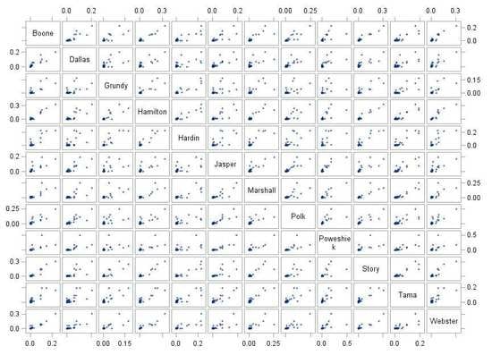
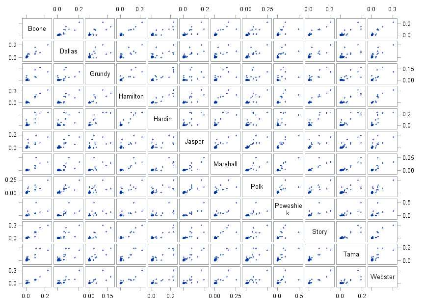
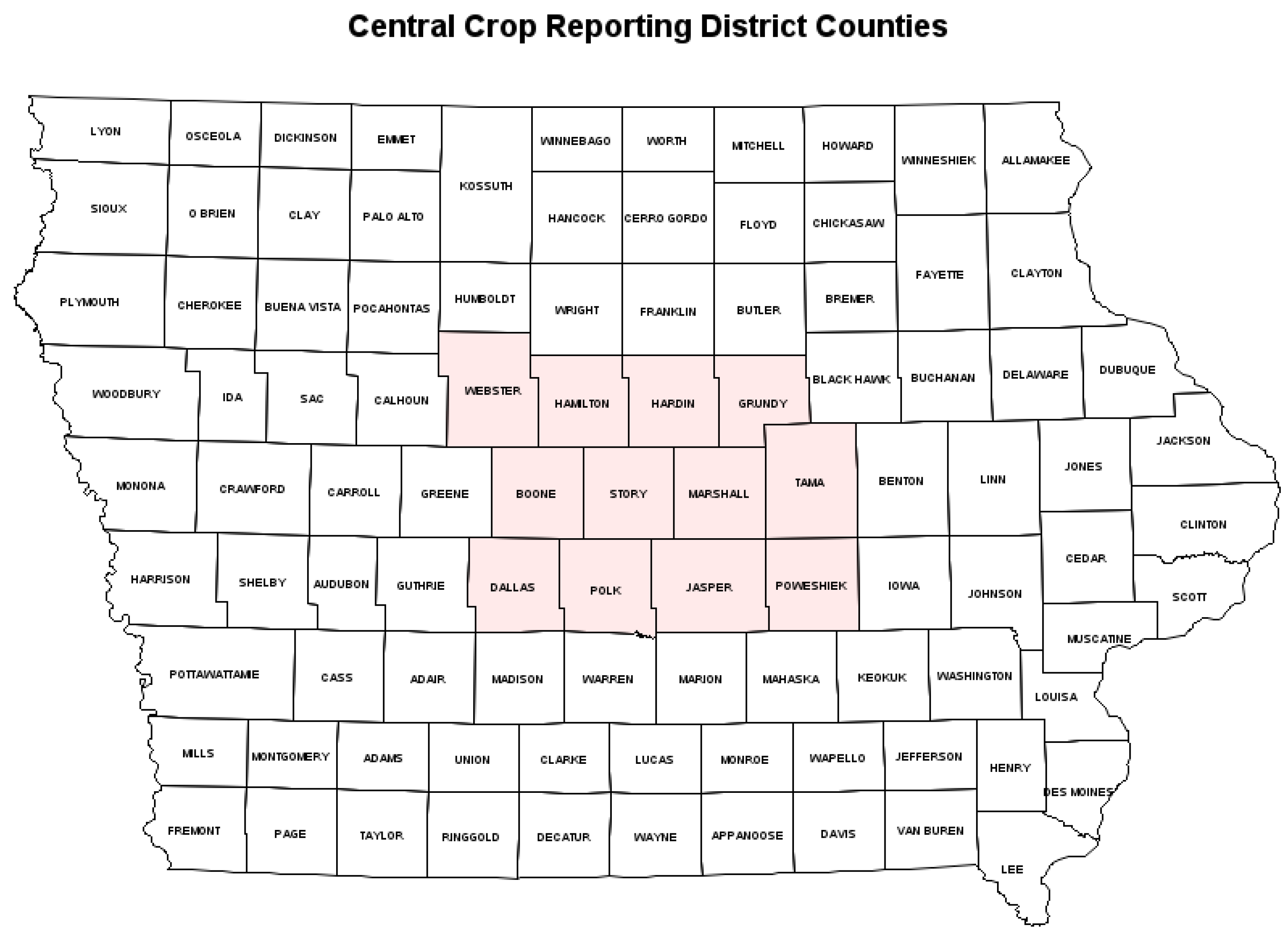
Corn is the largest US crop and currently accounts for about $40 billion in liability on 70 million acres each year in the US federal crop insurance program. Iowa is a major corn growing state in the US, making an ideal case study for considering alternative metrics of risk. We utilized the annual loss-cost ratios collected over the 1981–2017 period for the Central Crop Reporting District (CRD) in Iowa. The LCRs were summed at the county level and represent coverage of corn across all plans and coverage levels. This district is comprised of 12 counties: Boone, Dallas, Grundy, Hamilton, Hardin, Jasper, Marshall, Polk, Poweshiek, Story, Tama, and Webster. The relevant Iowa counties are illustrated in Figure 4. One would anticipate LCRs across these individual counties to be highly correlated (dependent). We would also anticipate a distribution that is heavily right-skewed, reflecting infrequent but very large loss events. Such events would typically correspond to poor weather such as drought or flood conditions, which is highly systemic in nature.

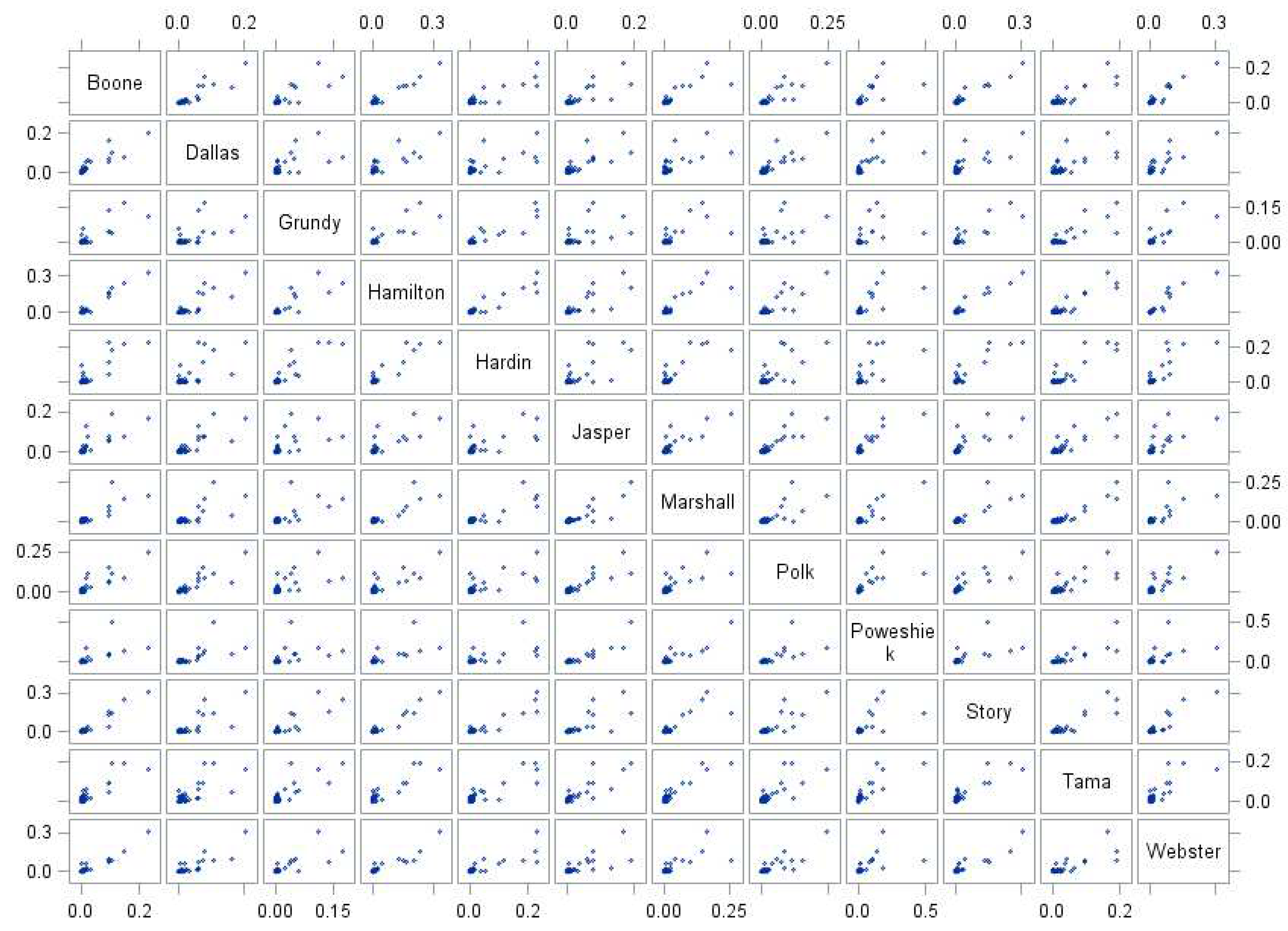
Figure 5 illustrates LCR values for each county. The values are suggestive of a high degree of positive skewness in the densities. The first step in our analysis involves fitting a parametric marginal density to each of the county-level LCR histories. We used the Akaike information criterion (AIC) to select the optimal density from among the following candidates—the Burr Type XII, the exponential, the gamma, the log-normal and the Weibull. We then considered chi-square and Kolmogorov–Smirnov (KS) goodness-of-fit tests to evaluate the optimal density.

Table 4. Goodness of fit criteria for alternative loss-cost distributions.

County	Marginal	AIC	BIC	Chi-Square	p-Value	Result	AD	CvM	KS	Result
Boone	Logn	−235.7045	−232.4294	7.6808	0.1040	FTR	0.5154	0.0710	0.1018	FTR
Dallas	Logn	−199.1769	−195.9017	3.4220	0.4898	FTR	0.2307	0.0295	0.0976	FTR
Grundy	Logn	−250.9037	−247.6286	3.9948	0.4067	FTR	−0.2656	0.0666	0.0955	FTR
Hamilton	Logn	−229.7353	−226.4601	5.3251	0.2555	FTR	0.3589	0.0447	0.0916	FTR
Hardin	Logn	−216.4420	−213.1668	2.4182	0.6593	FTR	0.3615	0.0496	0.0927	FTR
Jasper	Logn	−214.9949	−211.7197	3.2070	0.5238	FTR	0.3755	0.0555	0.0886	FTR
Marshall	Logn	−229.5464	−226.2712	2.7523	0.6001	FTR	0.2472	0.0403	0.0929	FTR
Polk	Weibull	−187.4824	−184.2073	5.3221	0.2558	FTR	0.4572	0.0837	0.1548	FTR
Poweshiek	Logn	−210.9589	−207.6837	5.3440	0.2538	FTR	0.4152	0.0656	0.0983	FTR
Story	Logn	−228.5102	−225.2350	5.4218	0.2467	FTR	0.4333	0.0606	0.1031	FTR
Tama	Logn	−187.8575	−184.5823	2.0636	0.7241	FTR	0.2076	0.0289	0.0730	FTR
Webster	Logn	−226.3786	−223.1034	3.0586	0.5481	FTR	0.5438	0.0808	0.1213	FTR

‘FTR’ indicates that the distribution was not rejected at the $\alpha =0.05$ or smaller level.

presents a summary of the analysis of parametric densities. In every case except for one (Polk County), the optimal parametric density is a log-normal. In the case of Polk County, the Weibull distribution had the minimal AIC value. The goodness of fit tests support the selected distributions in every case.

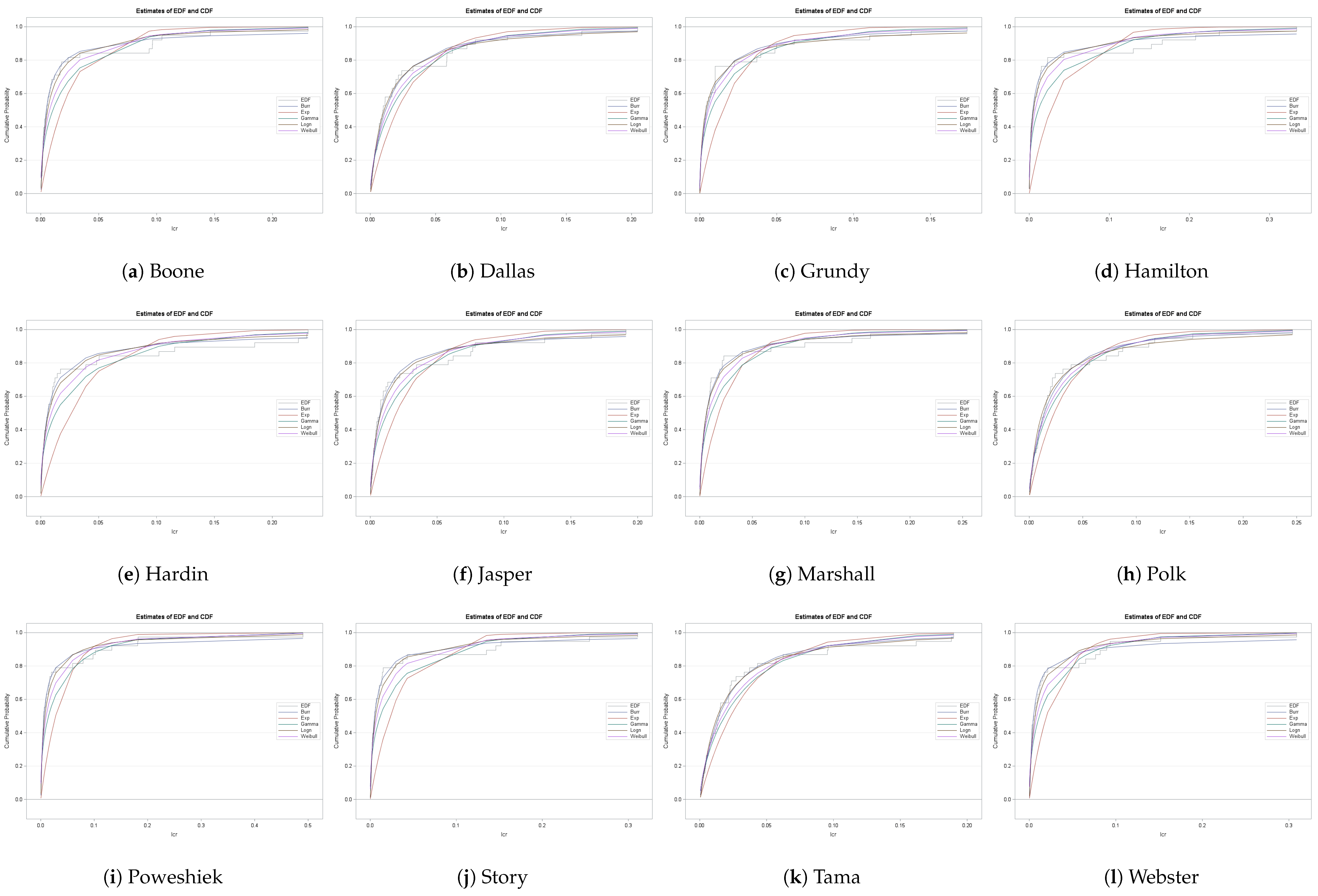
Figure 6 presents the estimated cumulative and empirical distribution functions for each county’s LCR. Figure 7 presents the estimated density functions. The right (positive) skewness associated with the LCR distributions is apparent and extreme, suggesting the potential for substantial VaR values. We evaluated VaR values for each county individually as well as for portfolios constructed from t and Gaussian copula estimates.

Table 5. t and Gaussian copula estimates.

County LCR	Boone	Dallas	Grundy	Hamilton	Hardin	Jasper	Marshall	Polk	Poweshiek	Story	Tama	Webster
Boone		0.9914	0.9753	0.9871	0.9783	0.9882	0.9874	0.9888	0.9822	0.9915	0.9835	0.9859
Dallas	0.8752		0.9614	0.9787	0.9719	0.9818	0.9796	0.9875	0.9773	0.9810	0.9748	0.9760
Grundy	0.6269	0.4647		0.9696	0.9780	0.9748	0.9768	0.9719	0.9646	0.9761	0.9734	0.9691
Hamilton	0.8359	0.7580	0.5911		0.9835	0.9830	0.9841	0.9789	0.9799	0.9886	0.9811	0.9872
Hardin	0.6871	0.6437	0.6444	0.8000		0.9675	0.9763	0.9714	0.9662	0.9792	0.9739	0.9753
Jasper	0.8106	0.7031	0.6581	0.8000	0.5692		0.9854	0.9909	0.9888	0.9869	0.9881	0.9781
Marshall	0.7695	0.6607	0.6199	0.7638	0.6230	0.7580		0.9809	0.9824	0.9855	0.9859	0.9819
Polk	0.7946	0.8384	0.5838	0.7372	0.6265	0.8730	0.7342		0.9834	0.9870	0.9799	0.9743
Poweshiek	0.7157	0.6539	0.4647	0.7031	0.5052	0.8132	0.7000	0.7919		0.9804	0.9857	0.9720
Story	0.8384	0.7250	0.6409	0.8480	0.6773	0.8480	0.7836	0.8527	0.7551		0.9853	0.9847
Tama	0.7189	0.5874	0.5120	0.7609	0.6472	0.8260	0.7695	0.7250	0.8235	0.7521		0.9721
Webster	0.7492	0.6773	0.5198	0.8310	0.6265	0.6054	0.6160	0.5692	0.5432	0.7095	0.4935

Upper diagonal elements correspond to t copula parameters and lower (shaded) diagonals correspond to Gaussian copula. The t copula has 9.3286 degrees of freedom, with an associated standard error of 1.7004.

presents estimates of the t and Gaussian copulas. Especially notable in the copula estimates is the relatively small degrees of freedom parameter estimate of 9.33, which suggests considerable tail dependence in the individual densities. This also suggests superior fit for the t copula in that it nests a Gaussian model, which is implied for large values of the degree of freedom parameter. This tail dependence is apparent in the copula dependence matrix estimates in Table 5. The dependence is much stronger in the case of the t copula. To capture asymmetric dependence we also estimated Clayton and Gumbel copulas. As noted, one would not typically expect multivariate Archimedean copulas to provide a flexible model of dependence as they have a single parameter. The dependence parameters for the Clayton and Gumbel copulas were, respectively, 0.9021 (with a standard error of 0.0360) and 5.1684 (with a standard error of 0.1894).

We used the copula and marginal density estimates to consider two alternative portfolios comprised of LCR values from the 12 counties. The first (portfolio 1) weights each county by 1/12 and the second (portfolio 2) considers a weighted average of experience, using the 2017 liability weights for each county. The estimates were quite similar, reflecting the fact that the liability of the portfolio was somewhat evenly distributed across the 12 counties.

VaR/return-period estimates are presented for each county individually and for each portfolio in

Table 6. VaR/return period estimates from individual counties and portfolios.

Density	t Copula				Gaussian Copula				Clayton Copula				Gumbel Copula
	1 in 100	1 in 50	1 in 10	1 in 5	1 in 100	1 in 50	1 in 10	1 in 5	1 in 100	1 in 50	1 in 10	1 in 5	1 in 100	1 in 50	1 in 10	1 in 5
Portfolio 1	0.43812	0.27920	0.08003	0.01131	0.43414	0.26790	0.07155	0.00824	0.22934	0.17712	0.08048	0.02090	0.42499	0.27078	0.06748	0.00830
Portfolio 2	0.46545	0.29400	0.08004	0.01074	0.44606	0.27757	0.07132	0.00770	0.24890	0.18486	0.08215	0.02005	0.43985	0.28077	0.06715	0.00779
Boone County, IA	0.37719	0.23366	0.05601	0.00574	0.31351	0.20307	0.05433	0.00593	0.32374	0.20598	0.05612	0.00588	0.31467	0.20361	0.05104	0.00588
Dallas County, IA	0.44318	0.28788	0.08190	0.01028	0.39576	0.25827	0.07993	0.01041	0.42397	0.24646	0.07936	0.01054	0.38156	0.25832	0.07464	0.01044
Grundy County, IA	0.57583	0.34552	0.06021	0.00388	0.54197	0.30180	0.05817	0.00395	0.44884	0.28862	0.05776	0.00392	0.52244	0.29673	0.05566	0.00390
Hamilton County, IA	0.84217	0.47607	0.07856	0.00496	0.71779	0.40096	0.08120	0.00515	0.82710	0.42288	0.08349	0.00513	0.70932	0.41233	0.07425	0.00511
Hardin County, IA	0.71455	0.40185	0.08318	0.00635	0.59942	0.37029	0.08031	0.00684	0.60625	0.36398	0.07669	0.00630	0.58270	0.34088	0.07709	0.00695
Jasper County, IA	0.42586	0.28374	0.07298	0.00796	0.40228	0.25647	0.06924	0.00785	0.45837	0.26377	0.06821	0.00778	0.38974	0.25304	0.06643	0.00797
Marshall County, IA	0.38769	0.26039	0.06036	0.00609	0.36363	0.21975	0.06003	0.00633	0.35996	0.24039	0.06057	0.00636	0.34208	0.21965	0.05539	0.00628
Polk County, IA	0.22775	0.18718	0.08725	0.01524	0.22851	0.17871	0.08526	0.01541	0.23674	0.18255	0.08589	0.01574	0.22151	0.17727	0.08187	0.01538
Poweshiek County, IA	0.62651	0.36814	0.08281	0.00743	0.54077	0.32652	0.08090	0.00780	0.51553	0.34094	0.08276	0.00797	0.49878	0.33102	0.07633	0.00758
Story County, IA	0.49854	0.28090	0.06481	0.00589	0.43580	0.26435	0.06522	0.00614	0.46184	0.27269	0.06719	0.00612	0.39927	0.26672	0.06006	0.00606
Tama County, IA	0.43648	0.28598	0.08735	0.01263	0.38722	0.25609	0.08625	0.01319	0.38582	0.25762	0.08349	0.01289	0.37834	0.25503	0.08220	0.01319
Webster County, IA	0.42491	0.24181	0.06379	0.00661	0.35799	0.23497	0.06233	0.00665	0.38993	0.24340	0.06269	0.00668	0.34738	0.23179	0.05799	0.00664

. Again, a 1 in 100 year return period represents the 99th percentile or VaR. The estimates are quite similar and reflect the high degree of spatial dependence inherent in the insurance experience. Insurers would expect to exceed LCR values of about 0.43–0.46 once every one-hundred years. The VaR values are slightly higher for the t-copula, reflecting the higher degree of tail dependence. In the loss ratio modeling, the worst case loss ratios were actually in the upper tail of the distribution. Thus we find that the Clayton copula, which can capture tail dependence only in the lower tail, results in much lower VaR estimates at almost all return periods except the one in five case. The results from the Gumbel copula are similar to those of the t and Gaussian copulas. The results from modeling of the loss cost ratios again indicate that the choice of the dependence structure can have an important effect on the total risk for the portfolio.

In sum, these empirical applications demonstrate several salient points related to modeling of extreme losses in crop insurance. Both the marginal model and dependence model matter. The loss history is characterized by several extreme losses that can dominate estimates of risk. But because crop yields are only measured once a year, and available data at the county level is limited, it can be difficult to accurately model the appropriate distributions using historical data. While these examples do not solve these fundamental issues, they do suggest additional research that may lead to better understanding of value-at-risk in crop insurance. However, they also highlight the need for continued investigation into the building blocks of the risk models: marginal distributions and dependence structures.

5. Conclusions

Accurate estimation of loss distributions is difficult when data is limited and theory provides little direction in the model space. Nonetheless, policymakers are often called upon to make decisions in this limited setting. Recent changes to farm legislation have prompted the RMA to make crop insurance available to a wider range of producers than ever before. Expansion of the program entails new actuarial developments for individual policies as well as construction of risk measures for the crop insurance portfolio. One such measure is value-at-risk; VaR gives the loss at high quantiles of the loss distribution. VaR is analogous to the return period or probable maximum loss as more commonly termed in insurance settings.

We examine VaR and PML under a number of alternative dependence scenarios. After modeling the marginal distributions of losses and loss-costs, we use independent, Gaussian, and t copulas to capture dependence among the factors in the portfolio. The algorithm of Embrechts et al. (2013) is used to estimate bounds on the VaR in what can be considered worst-case dependence scenarios. We find that there is a large degree of model risk arising from the dependence structure. Differences in the dependence models should be taken into account when making reserving decisions or forecasting future outlays for the crop insurance program.

These results also serve to highlight the intricacies involved in determining the degree of systemic risk inherent in crop insurance portfolios. Both the marginal distributions and dependence structure can exhibit non-stationary behavior; much attention has been paid to normalizing observed data so that loss distributions can be obtained. Unfortunately, researchers and actuaries must provide loss estimates in situations where the model space is large, but available data is small. New techniques for borrowing information across space have brought increased accuracy in ratemaking. A useful comparison to the top-down approach to VaR would be to compare with bottom-up modeling of the yield risk factors and see if the two methods arrive at roughly the same estimates of portfolio risk.

Several extensions could be made to the methods presented here. Accurate modeling of the marginal distributions is important in calculation of VaR. We have assumed that the distributions of losses and loss costs are stable over time. Moreover, we have not dealt with bounding of the loss distributions. A useful improvement would be to consider marginals that take into account bounds on losses, the possibility of zero inflation (zero loss can be common in crop insurance portfolios, especially at low coverage levels), and changes over time. Although not considered directly in this paper, it seems reasonable that a large portion of the model risk could arise from the marginal models.

Crop insurance is not only a major mechanism for agricultural risk management in the United States, but has become a worldwide phenomenon. Mahul and Stutley (2010) note an increasing reliance on government supported agricultural insurance in developing countries. Agricultural insurance programs, whether completely public, private, or a combination of the two, have a variety of reinsurance schemes. These can vary from full public reinsurance to private reinsurance to coinsurance pools and other arrangements. Policymakers considering public agricultural insurance as a policy tool need accurate estimates of the risk from such programs in making decisions. Value-at-risk is one risk measure for informing policy debates and the design of fiscally sustainable agricultural insurance programs.

References

- Aas, Kjersti, and Giovanni Puccetti. 2014. Bounds on total economic capital: The DNB case study. Extremes 17: 693–715. [Google Scholar] [CrossRef]
- Cleveland, William S., and Susan J. Devlin. 1988. Locally weighted regression: An approach to regression analysis by local fitting. Journal of the American Statistical Association 83: 596–610. [Google Scholar] [CrossRef]
- Cope, E.W., G. Mignola, G. Antonini, and R. Ugoccioni. 2009. Challenges in measuring operational risk from loss data. Journal of Operational Risk 4: 3–27. [Google Scholar] [CrossRef]
- Elaine Hungerford, Ashley, and Barry Goodwin. 2014. Big assumptions for small samples in crop insurance. Agricultural Finance Review 74: 477–91. [Google Scholar] [CrossRef]
- Embrechts, Paul, Giovanni Puccetti, and Ludger Rüschendorf. 2013. Model uncertainty and VaR aggregation. Journal of Banking & Finance 37: 2750–64. [Google Scholar]
- Frees, Edward W., and Ping Wang. 2006. Copula credibility for aggregate loss models. Insurance: Mathematics and Economics 38: 360–73. [Google Scholar] [CrossRef]
- Gallagher, Paul. 1986. US corn yield capacity and probability: Estimation and forecasting with nonsymmetric disturbances. North Central Journal of Agricultural Economics 8: 109–22. [Google Scholar] [CrossRef]
- Goodwin, Barry K., and Ashley Hungerford. 2014. Copula-based models of systemic risk in US agriculture: Implications for crop insurance and reinsurance contracts. American Journal of Agricultural Economics 97: 879–96. [Google Scholar] [CrossRef]
- Goodwin, Barry K., and Alan P. Ker. 1998. Nonparametric estimation of crop yield distributions: Implications for rating group-risk crop insurance contracts. American Journal of Agricultural Economics 80: 139–53. [Google Scholar] [CrossRef]
- Hayes, Dermot J., Sergio H. Lence, and Chuck Mason. 2003. Could the government manage its exposure to crop reinsurance risk? Agricultural Finance Review 63: 127–42. [Google Scholar] [CrossRef]
- Holly Wang, H., and Hao Zhang. 2003. On the possibility of a private crop insurance market: A spatial statistics approach. Journal of Risk and Insurance 70: 111–24. [Google Scholar] [CrossRef]
- Hurvich, Clifford M., Jeffrey S. Simonoff, and Chih-Ling Tsai. 1998. Smoothing parameter selection in nonparametric regression using an improved Akaike information criterion. Journal of the Royal Statistical Society: Series B (Statistical Methodology) 60: 271–93. [Google Scholar] [CrossRef]
- Ker, Alan P., and Keith Coble. 2003. Modeling conditional yield densities. American Journal of Agricultural Economics 85: 291–304. [Google Scholar] [CrossRef]
- Ker, Alan P., and Pat McGowan. 2000. Weather-based adverse selection and the US crop insurance program: The private insurance company perspective. Journal of Agricultural and Resource Economics 25: 386–410. [Google Scholar]
- Ker, Alan P., Tor N. Tolhurst, and Yong Liu. 2015. Bayesian Estimation of Possibly Similar Yield Densities: Implications for Rating Crop Insurance Contracts. American Journal of Agricultural Economics 98: 360–82. [Google Scholar] [CrossRef]
- Mahul, Olivier, and Charles J. Stutley. 2010. Government Support to Agricultural Insurance: Challenges and Options for Developing Countries. Washington, DC: The World Bank. [Google Scholar]
- Mainik, Georg, and Paul Embrechts. 2013. Diversification in heavy-tailed portfolios: Properties and pitfalls. Annals of Actuarial Science 7: 26–45. [Google Scholar] [CrossRef]
- Nikoloulopoulos, Aristidis K., Harry Joe, and Haijun Li. 2012. Vine copulas with asymmetric tail dependence and applications to financial return data. Computational Statistics & Data Analysis 56: 3659–73. [Google Scholar]
- Odening, Martin, and Zhiwei Shen. 2014. Challenges of insuring weather risk in agriculture. Agricultural Finance Review 74: 188–99. [Google Scholar] [CrossRef]
- Okhrin, Ostap, Martin Odening, and Wei Xu. 2013. Systemic weather risk and crop insurance: The case of China. Journal of Risk and Insurance 80: 351–72. [Google Scholar] [CrossRef]
- Okhrin, Ostap, Yarema Okhrin, and Wolfgang Schmid. 2013. 2013 On the structure and estimation of hierarchical Archimedean copulas. Journal of Econometrics 173: 189–204. [Google Scholar] [CrossRef]
- Ozaki, Vitor A., and Ralph S. Silva. 2009. Bayesian ratemaking procedure of crop insurance contracts with skewed distribution. Journal of Applied Statistics 36: 443–52. [Google Scholar] [CrossRef]
- Park, Eunchun, B. Wade Brorsen, and Ardian Harri. 2018. Using Bayesian Kriging for Spatial Smoothing in Crop Insurance Rating. American Journal of Agricultural Economics 101: 330–51. [Google Scholar] [CrossRef]
- Patton, Andrew J. 2009. Copula—Based models for financial time series. In Handbook of Financial Time Series. Berlin: Springer, pp. 767–85. [Google Scholar]
- Porth, Lysa, Milton Boyd, and Jeffrey Pai. 2016. Reducing Risk Through Pooling and Selective Reinsurance Using Simulated Annealing: An Example from Crop Insurance. The Geneva Risk and Insurance Review 41: 163–91. [Google Scholar] [CrossRef]
- Puccetti, Giovanni, and Ludger Rüschendorf. 2012. Computation of sharp bounds on the distribution of a function of dependent risks. Journal of Computational and Applied Mathematics 236: 1833–40. [Google Scholar] [CrossRef]
- Puccetti, Giovanni. 2013. Sharp bounds on the expected shortfall for a sum of dependent random variables. Statistics & Probability Letters 83: 1227–32. [Google Scholar]
- Ramsey, A. Ford, Barry K. Goodwin, and Sujit K. Ghosh. 2019. How High the Hedge: Relationships between Prices and Yields in the Federal Crop Insurance Program. Journal of Agricultural and Resource Economics 44. forthcoming. [Google Scholar]
- Risk Management Agency. 2018. Summary of Business. Available online: https://prodwebnlb.rma.usda.gov/apps/SummaryOfBusiness (accessed on 3 January 2019).
- Sherrick, Bruce J., Fabio C. Zanini, Gary D. Schnitkey, and Scott H. Irwin. 2004. Crop insurance valuation under alternative yield distributions. American Journal of Agricultural Economics 86: 406–19. [Google Scholar] [CrossRef]
- Sklar, Abe. 1959. Distribution Functions in n Dimensions and Their Margins. Statistics Publications, University of Paris 8: 229–31. [Google Scholar]
- Tack, Jesse B., and David Ubilava. 2013. The effect of El Niño Southern Oscillation on US corn production and downside risk. Climatic Change 121: 689–700. [Google Scholar] [CrossRef]
- Tamakoshi, Go, and Shigeyuki Hamori. 2014. The conditional dependence structure of insurance sector credit default swap indices. The North American Journal of Economics and Finance 30: 122–32. [Google Scholar] [CrossRef]
- Tolhurst, Tor N., and Alan P. Ker. 2014. On technological change in crop yields. American Journal of Agricultural Economics 97: 137–58. [Google Scholar] [CrossRef]
- Yang, Lu, Xiao Jing Cai, Mengling Li, and Shigeyuki Hamori. 2015. Modeling dependence structures among international stock markets: Evidence from hierarchical Archimedean copulas. Economic Modelling 51: 308–14. [Google Scholar] [CrossRef]
- Zhu, Ying, Barry K. Goodwin, and Sujit K. Ghosh. 2011. Modeling yield risk under technological change: Dynamic yield distributions and the US crop insurance program. Journal of Agricultural and Resource Economics 36: 192–210. [Google Scholar]