Predicting Micro-Enterprise Failures Using Data Mining Techniques


Institute of Statistics and Demography, Warsaw School of Economics, Warsaw 02-554, Poland
J. Risk Financial Manag. 2019, 12(1), 30; https://doi.org/10.3390/jrfm12010030
Submission received: 30 December 2018
/
Revised: 27 January 2019
/
Accepted: 3 February 2019
/
Published: 10 February 2019
(This article belongs to the Special Issue Empirical Finance)
Abstract
:Research analysis of small enterprises are still rare, due to lack of individual level data. Small enterprise failures are connected not only with their financial situation abut also with non-financial factors. In recent research we tend to apply more and more complex models. However, it is not so obvious that increasing complexity increases the effectiveness. In this paper the sample of 806 small enterprises were analyzed. Qualitative factors were used in modeling. Some simple and more complex models were estimated, such as logistic regression, decision trees, neural networks, gradient boosting, and support vector machines. Two hypothesis were verified: (i) not only financial ratios but also non-financial factors matter for small enterprise survival, and (ii) advanced statistical models and data mining techniques only insignificantly increase the prediction accuracy of small enterprise failures. Results show that simple models are as good as more complex model. Data mining models tend to be overfitted. Most important financial ratios in predicting small enterprise failures were: operating profitability of assets, current assets turnover, capital ratio, coverage of short-term liabilities by equity, coverage of fixed assets by equity, and the share of net financial surplus in total liabilities. Among non-financial factors only two of them were important: the sector of activity and employment.
1. Introduction
Since the announcement of the Altman’s Z-Score model (Altman 1968), a large number of statistical bankruptcy prediction studies were written using the traditional methods, like discriminant analysis (Back et al. 1996), logistic regression (Aziz and Dar 2006; Back et al. 1996), and probit analysis (Zmijewski 1984). Recent studies in this area focus on more advanced and sophisticated methods, like case-based reasoning (Sartori et al. 2016), genetic algorithms (Back et al. 1996), and neural networks (Blanco-Oliver et al. 2013) or support vector machines (Kim and Sohn 2010).
Sartori et al. (2016) applied the case-based reasoning (CBR) paradigm to forecast the bankruptcy and compared the results received with the Z-Score model. The CBR method turned out to be good in predicting bankruptcy. The authors found that this approach could be useful to cluster enterprises according to opportune similarity metrics.
Genetic algorithms (GAs) were another method used in SMEs’ default prediction analysis. Gordini (2014) compared the potential of genetic algorithms with two other methods: logistic regression (LR) and support vector machine (SVM). The results obtained suggest that GAs are a very effective and promising method in assessing the probability of SMEs bankruptcy compared with LR and SVM, especially in reducing type II misclassification rates. The author also investigated whether the size of firms and the geographical area of their operation can influence the accuracy of the models and, again, the results obtained from separate models built to custom for separate geographical areas show that GAs prediction accuracy in each area is superior to that of the other models.
Lahmiri (2016a) in this paper compared several predictive models that combine features selection techniques with data mining classifiers in the context of credit risk assessment in terms of accuracy, sensitivity, and specificity. He used the support vector machine (SVM), back-propagation neural network, radial basis function neural network, linear discriminant analysis, and naive Bayes classifier. Results from three datasets using a 10-fold cross-validation technique showed that the SVM provides the best accuracy. The SVM seems to be an attractive classifier to be used in real applications for bankruptcy prediction. In his later works Lahmiri (2017) proposed a two-step system to improve prediction of telemarketing outcomes and to help the marketing management team effectively manage customer relationships in the banking industry. Several neural networks were trained with different categories of information to make initial predictions. Next, all initial predictions were combined by a single neural network to make a final prediction. Empirical results indicated that the two-step system presented performs better than all its individual components. According to author the proposed two-step system seems to be robust to noisy and nonlinear data, easy to interpret, suitable for large and heterogeneous marketing databases, fast and easy to implement.
Sohn et al. (2016) proposed an approach based on fuzzy logistic regression that can be used in the default prediction models. Moreover, the authors showed that the proposed approach outperforms the logistic regression model in terms of discriminatory power. Similarly, Chaudhuri and De (2011) used the fuzzy support vector machine which outperformed traditional bankruptcy prediction methods.
Traditional analysis of company financial condition is based on financial factors. However, it is worth considering whether other indicators can be significant. This problem was addressed by few researchers. Jiménez and Saurina (2004) discussed the role of a limited set of variables, namely: collateral, type of lender and bank-borrower relationship. According to their results, collateralized loans have higher probability of default and loans granted by savings banks are riskier. Additionally, authors found that a close relationship between the bank and the customer increases the willingness to take more risk.
Psillaki et al. (2010) showed that non-financial performance indicators are useful ex ante determinants of business failure. Using the companies’ datasets from three different French manufacturing industries they proved that managerial inefficiencies are an important ex ante indicator of a firm’s financial risk. The results suggest that more efficient firms, as well as firms with more liquid assets are less likely to fail. A similar approach was taken by Fabling and Grimes (2005), who used regional as well as national data. They analyzed the role of property prices, which influenced the collateral values. According to the authors’ findings the interactions between economic activity, leverage and property price (collateral) shocks indicate that region-specific shocks can compound into significant localized economic cycles.
A variation of the approach was suggested by Kalak and Hudson (2016). Using a US dataset of companies that became insolvent in between 1980 and 2013, the authors built four discrete-time duration-dependent hazard models for SMEs, micro-, small-, and medium-sized companies. Authors indicated that there are significant differences between micro and small firms and these categories should be considered separately when building the credit risk models. Analogous to Kalak and Hudson (2016), Gupta et al. (2015) investigated how the SMEs size can affect credit risk. Their research results suggest that separate models for micro firms are desired. In case of small and medium companies, there is no such a need as the determinants present similar level of hazard.
Ong et al. (2005) analyzed usage of the genetic programming in building credit scoring models. According to their results, model built with genetic programming (GP) outperformed models built with other methods, namely the artificial neural networks ANN, decision trees, rough sets, and logistic regression. Huang et al. (2006), proposed building a two-stage genetic programming (2SGP) model as it achieves better results than other models. Berg (2007) used different accounting-based models for bankruptcy prediction. Obtained results suggest that generalized additive models outperform models like linear discriminant analysis, generalized linear models and neural networks. In order to identify defaulted SMEs, Calabrese et al. (2015) investigated a binary regression accounting-based model. Results obtained suggest that their approach outperformed the classical logistic regression model for different default horizons considered.
Lahmiri (2016b) also compared the forecasting ability of different data mining techniques like the backpropagation neural network (BPNN) and the nonlinear autoregressive moving average with exogenous inputs (NARX) network trained with different optimization algorithms. The simulation results showed that in general the NARX which is a dynamic system outperforms the popular BPNN. In addition, conjugate gradient algorithms provide better prediction accuracy than the Levenberg-Marquardt algorithm widely used in the literature in modeling exponential signals. However, the LM performed the best when used for forecasting the Moroccan and South African stock price indices under both the BPNN and NARX systems.
In his later paper Lahmiri (2016c) compared the accuracy of three hybrid intelligent systems in forecasting ten international stock market indices; namely the CAC40, DAX, FTSE, Hang Seng, KOSPI, NASDAQ, NIKKEI, S and P 500, Taiwan stock market price index, and the Canadian TSE. Based on out-of-sample simulation results, he found that contrary to the literature GA-TDNN significantly outperforms GA-ATDNN. In addition, ANFIS was found to be more effective in forecasting CAC40, FTSE, Hang Seng, NIKKEI, Taiwan, and the TSE price level. In contrary, GA-TDNN and GA-ATDNN were found to be superior to ANFIS in predicting DAX, KOSPI, and NASDAQ future prices.
In Poland the first corporate bankruptcies took place in 1990 after start of economic transformation. Predicting corporate bankruptcies in Poland have been of interest to the researchers since 1990s, but since then the studies dealing with this subject have been numerous. For this reason, only an overview of the selected literature on this topic is mentioned below. The very first research was aimed at applying foreign models, like the Altman model, to predict bankruptcies of Polish enterprises (Mączyńska 1994). At the same time the Polish researchers started using financial ratios analysis (Wędzki 2000; Stępień and Strąk 2003; Prusak 2005), and build first national models (Pogodzińska and Sojak 1995; Gajdka and Stos 1996; Hadasik 1998; Wierzba 2000). Due to the limited access to the data, these models were based on small samples and mainly on multivariate linear discriminant analysis. Later on other models were applied and the sizes of the data samples were larger (Hołda 2001; Sojak and Stawicki 2000; Mączyńska 2004; Appenzeller and Szarzec 2004; Korol 2004; Hamrol et al. 2004; Prusak 2005; Jagiełło 2013). Next the newer statistical techniques also were used, such as the logit models (Gruszczyński 2003; Michaluk 2003; Wędzki 2004; Stępień and Strąk 2004; Prusak and Więckowska 2007; Jagiełło 2013; Pociecha et al. 2014; Karbownik 2017), neural networks, other genetic algorithms, classification trees or survival analysis using the Cox model (Michaluk 2003; Korol 2004; Pociecha et al. 2014; Gąska 2016; Ptak-Chmielewska 2016), the k-nearest neighbors method, kernel classifiers, random forests, Bayesian networks, support vectors, and fuzzy logic and methods for ensemble models (Korol 2010b; Gąska 2016, Zięba et al. 2016). In addition to universal models, many sectoral models were created (Brożyna et al. 2016; Balina and Bąk 2016; Jagiełło 2013; Karbownik 2017). The criterion of enterprise size were utilized (Jagiełło 2013). Not only financial ratios, but also non-financial factors and macroeconomic variables were used as explanatory variables to construct the models of enterprise bankruptcy risk assessment (Korol 2010a; Ptak-Chmielewska and Matuszyk 2017). In addition, the risk of bankruptcy depends on the economic cycle and therefore suggested that enterprise bankruptcy forecasting models should consider measures showing changes in economic conditions (Pociecha and Pawełek 2011).
Błażej (2018) Prusak’s article Review of Research into Enterprise Bankruptcy Prediction in Selected Central and Eastern European Countries (International Journal of Financial Studies, published: 22 June 2018) used a literature review as a research method. The author presented the results of the research on corporate bankruptcy prediction related to highly-developed countries, which reached many years back and covered the main research and a comparative basis for the Central and Eastern European countries. Collected material included countries which founded the CMEA (Council for Mutual Economic Assistance) or which later emerged as a result of its collapse (Poland, Lithuania, Latvia, Estonia, Ukraine, Hungary, Russia, Slovakia, Czech Republic, Romania, Bulgaria, Belarus). Information on the publications covered the period of Q4 2016–Q3 2017 from Google Scholar and ResearchGate databases. Based on such wide literature review author proposed the ratings described below (Prusak 2018, p. 17):
- Rating 0—There are no studies in enterprise bankruptcy risk prediction in the given country.
- Rating 1—Analyses are conducted to assess the risk of bankruptcy of enterprises using only foreign models in the country concerned.
- Rating 2—Both national and foreign models are used to assess the risk of business insolvency in the country concerned, with national models being constructed using less sophisticated statistical methods, i.e., linear multidimensional discriminant analysis, logit and probit methods, etc.
- Rating 3—Both national and foreign models are used to assess the risk of business insolvency in the country concerned, with national models being constructed using also more advanced methods: artificial neural networks, genetic algorithms, the support vector method, fuzzy logic, etc. Moreover, national sectoral models are also estimated.
- Rating 4—The most advanced methods are used in enterprise bankruptcy risk forecasting in the country concerned and the researchers propose new solutions that affect the development of this discipline.
According to author’s assessment Poland grade was the highest 4.0 with following comment (Prusak 2018, p. 17): “Numerous studies have been performed in this area. Many national and sectoral models have been evaluated using the latest statistical methods. Both financial and non-financial information have been used as explanatory variables. Additionally, attention was paid to the impact of the economic climate on the efficiency of models for the forecasting of enterprise insolvency.”
Other rated countries got grades from the lowest: Belarus (1.5), Bulgaria (1.5), Latvia (2.0), Romania (2.0), Lithuania (2.5), Ukraine (2.5), medium grade like: Estonia (3.0), Hungary (3.0), Russia (3.0), Slovakia (3.5) to the highest: Czech Republic (4.0).
In my research I focused on two research hypothesis to be verified:
Hypothesis 1 (H1):
Not only financial ratios but also non-financial factors matter for small enterprises survival.
Hypothesis 2 (H2):
Advanced statistical models and data mining techniques only insignificantly increase the prediction accuracy of small enterprise failures modeling.
2. Materials and Methods
In this research the sample of 806 small enterprises was used including 311 bankruptcies and 495 non-bankrupted enterprises for bankruptcy prediction. Sample covered the equal proportion of enterprises from sectors: industry, trade and services. The financial statements covered the period of 2008−2010. The bankruptcy events took place between 2009 and 2012, a 12-month observation period was considered. The data were kindly provided by a consultancy firm operating on the Polish market. From a long list of financial ratios only 16 were selected based on univariate analysis:
| Mean | SD | ||
| w1 | Current liquidity | 1.877 | 1.584 |
| w2 | Quick ratio | 1.351 | 1.236 |
| w3 | Liquidity cash | 0.406 | 0.655 |
| w4 | Capital share in assets | 0.149 | 0.326 |
| w5 | Gross margin | 0.058 | 0.134 |
| w6 | Operating profitability of sales | 0.022 | 0.101 |
| w7 | Operating profitability of assets | 0.040 | 0.189 |
| w8 | Net profitability of equity | 0.180 | 0.583 |
| w9 | Assets turnover | 2.419 | 1.484 |
| w10 | Current assets turnover | 3.860 | 2.308 |
| w11 | Receivables turnover | 10.521 | 10.458 |
| w12 | Inventory turnover | 4.740 | 3.689 |
| w13 | Capital ratio | 0.336 | 0.328 |
| w14 | Coverage of short-term liabilities by equity | 1.592 | 2.294 |
| w15 | Coverage of fixed assets by equity | 2.948 | 5.294 |
| w16 | Share of net financial surplus in total liabilities | 0.226 | 0.473 |
There are 16 administrative regions in Poland, so called voivodeships. Those 16 regions were grouped according to hierarchical clustering into 4 groups (low risk, lower-medium, higher-medium, and high risk of bankruptcy) to create the variable: region. All together five non-financial factors were used: sector of the company’s activity (industry, trade, services); company’s legal form (self-employed, joint stock company, limited liability company, limited partnership company, other); region (grouped as mentioned above); age of the company (in years); employment (number of employed workers at the date of financial statement).
The sample was partitioned into a training sample (70%) and a test sample (30%) with the same proportion of bankruptcy events in each sample.
Models used for estimation and comparison consisted of six different models: logistic regression with interval variables, logistic regression with discretized variables, decision tree, gradient boosting, neural network, and support vector machines.
2.1. Logistic Regression
The logistic regression function is S-shaped and described by the following formula:
where:
- β0—intercept,
- βI—coefficients (i = 1, 2, …, k),
- xi—explanatory variables (i = 1, 2, …, k).
The P(Y = 1) takes the values from interval [0; 1]. The cut-off point is an important element in the logistic regression model. Estimation based on a balanced sample usually takes the 0.5 as the cut-off value. The structure of the sample (the percentage of bankrupted enterprises) determines the cut-off value. Interpretation of results is usually based on odds ratios (the ratio of odds in two groups or in change of one unit in explanatory variable). Logistic regression requires a number of different assumptions to be fulfilled. The most important assumptions are: randomness of the sample, a large sample, no collinearities in explanatory variables, and independence of observations.
2.2. Decision Tree
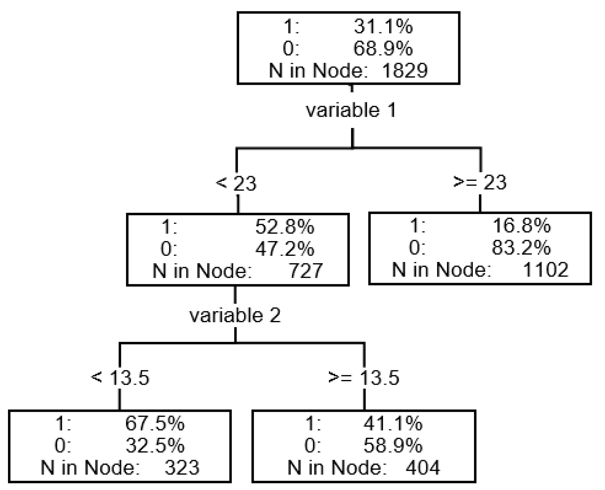
A decision tree is a tool mainly used in hierarchical segmentation (division) of the dataset. The main element is the so-called root that includes the entire dataset. Subsequent splits of the data (observations) are carried out in the so-called nodes, or segments, according to the rules created on the basis of the values of explanatory variables. A segment that is subdivided into subsegments is being referred to as the parent node (or intermediate node) and the subsegments as children nodes. The tree branch creates a node with further subsegments. A leaf (group) is the final segment that is no longer divided. Each observation from the output node is assigned to only one final leaf. The decision tree contains intermediate and final nodes, while the decision tree model contains only the final leaves that are used to predict or classify data (see Figure 1).
In order for decision trees to be used, a large collection of observations is required, as well as sufficiently numerous cases for the dependent variable. Any (very) unusual observations may distort the results, though this is not a major risk. A big risk in building the tree is overfitting, which can cause instability of the model. The decision tree, unlikely the binary logistic regression, does not contain any equations or coefficients, it is based only on the rules of dividing the dataset into separate groups. As estimation of probabilities posteriori probabilities for each leaf are used. The rules generated by the model from the learning set can be used for prediction (resulting in binary decisions).
The basic ways to measure the quality of the division for binary dependent variables or discrete dependent variables with several categories include:
- The degree of separation achieved by the division (measured by the Pearson chi-squared test),
- The degree of pollution reduction achieved by the division (measured by the reduction of entropy or by the Gini coefficient).
The stopping criteria may be the following: the minimal number of observations in any final leaf, the critical size of any node, the number of splits in any path. After building a tree, it should be pruned into an optimal size. The advantages of a decision tree are twofold: the results are easily interpretable and the model is flexible. Additionally, decision trees are not sensitive to missing data and do not require the normality of distributions or the equality of covariance matrices (as discriminant analysis does). The explanatory variables may differ in character, being either qualitative or quantitative. Decision trees automatically select important variables and may explain non-linear dependencies. The disadvantage of the decision trees is the fact that they can prove unstable and sensitive to the size of the training sample, validation or test sample results. The large size of the training sample is critical. Probabilities are approximated on the final leaf level. Overtraining is quite common in decision trees and the results for the training sample are usually much better than for the testing sample. All those disadvantages must be considered while building a model.
2.3. Gradient Boosting
Nowadays, a more popular method is the random forest, initially proposed by Breiman. It is a method that takes together many classification trees. Firstly, we draw K bootstrap samples, then we create a classification tree for each of them in such a way that in each node we draw m (fewer than the number of all features) features which will participate in the selection of the best division. Trees are built without pruning. Finally, the observations are classified by the voting method. The only parameter of the method is the m coefficient, which should be much smaller than the dimension of data. The ease and speed with which random forests can be created makes them a feasible option even for very large data. Random forests are currently one of the most efficient classification methods, apart from the SVM and boosting. The boosting method makes it possible to cope with an opposite situation: it allows to aggregate many stable but less efficient classifiers (weak learners). The classification abilities of weak learners are small—the probability of correct classification slightly exceeds 1/2. The main idea is that in the iteration process the observations should be assigned weights which suggest to weak learners on which examples they should concentrate in their next approach to the classification task. The final decision regarding the classification of observations is made in majority voting. The main feature of boosting is the ability to decrease the training error: a group of weak learners acts together as a single good learner. What is more important, the error decreases exponentially, which is very important in practical usage. An additional advantage is that the boosting algorithms are not subject to overfitting.
2.4. Neural Network
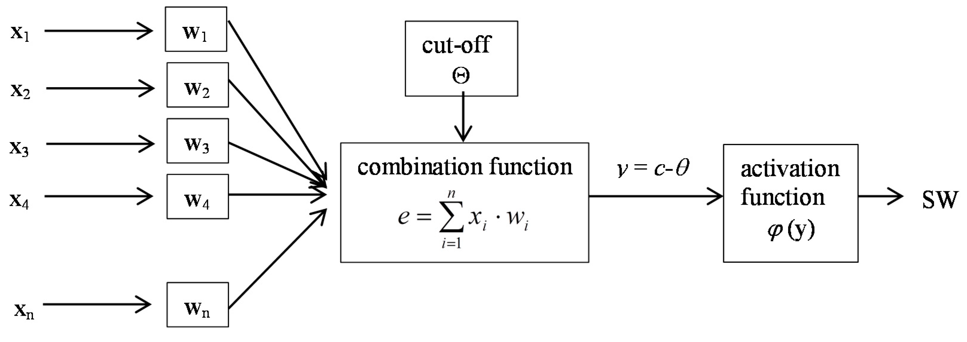
The neural network, i.e., the fourth analyzed method, is formed by the neurons (information processing elements) along with the connections among them (weights modified during the learning process). This network is a simplified model of the human brain. A neuron contains many inputs xi, where i = 1, 2, ..., n and one output. Neural inputs are selected by the explanatory variables. When neural networks are used to forecast the risk of bankruptcy, these are typically financial ratios. Each input variable is assigned a specific weight wi. Once the weights are determined, the total neuron activation (e) is calculated as the sum of the product of the explanatory variables and their weights assigned. Then y is calculated, which is the difference between the value of e and the threshold value Θ. The output signal depends on the neuron activation and the activation function φ(y). The form of this function determines the neuron type (see Figure 2).
In practice, artificial neural networks are usually made of a large number of interconnected neurons. We can distinguish the following neural networks:
- -
- double layer neural networks—consisting of the input and output layers;
- -
- multi-layered neural networks—consisting of input and output layers and hidden layers between them.
In predicting the bankruptcy of enterprises multi-layer perceptron (MLP) neural networks are frequently used. Neural networks are flexible and they quickly adapt to changes. They are resistant to any chaotic information and do not require assumptions like normality etc. The explanatory variables can be both qualitative and quantitative in type. Neural networks enable the modeling of any type of non-linear dependencies in the data.
Unfortunately, neural network models also have significant limitations. The long-term learning process for networks with extensive structures prevents the model from achieving an optimal level of error reduction. The weights selection process is difficult and complex. Neural networks do not select explanatory variables for the model. The analyst conducts a selection of explanatory variables by himself. Similarly as in the case of decision trees, there is a risk of overtraining. Selecting network architecture is a subjective choice. The worst disadvantage of the neural networks approach is the fact that they operate on the “black box” basis—without the ability to provide the rules that resulted in the obtained outcome. In neural network model all variables were used. Results are not as easily interpretable as in the decision tree model.
2.5. Support Vector Machines
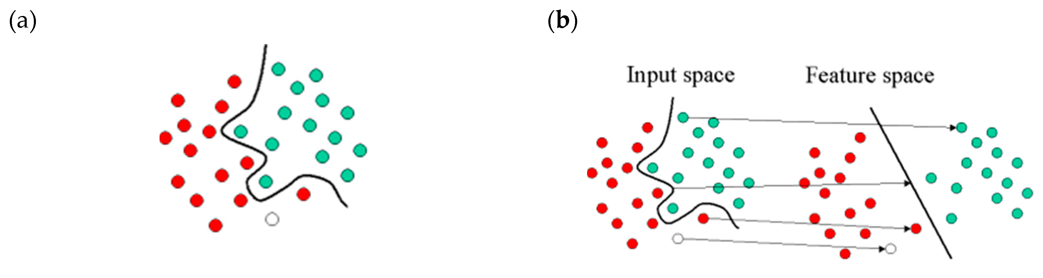
Support vector machines are based on the concept of decision planes that define decision boundaries. A decision plane is one that separates between a set of objects having different class memberships. The classic example of a separation is a linear classifier that separates a set of objects into their respective groups with a line. Most classification tasks, however, are not that simple, and often more complex structures are needed in order to make an optimal separation, i.e., to correctly classify new objects (test cases) on the basis of the examples that are available (train cases). This situation is depicted in the illustration below (Figure 3a). A full separation of the “green” and “red” objects would require a curve (which is more complex than a line). Classification tasks based on drawing separating lines to distinguish between objects of different class memberships are known as hyperplane classifiers. Support vector machines handle such tasks. The illustration below (Figure 3b) shows the basic idea behind support vector machines. The original objects (left side of the schematic) mapped, i.e., rearranged, using a set of mathematical functions, known as kernels. The process of rearranging the objects is known as mapping (transformation).
The support vector machine (SVM) is primarily a classier method that performs classification tasks by constructing hyperplanes in a multidimensional space that separates cases of different class labels. SVM supports both regression and classification tasks and can handle multiple continuous and categorical variables. For categorical variables a dummy variable is created with case values as either 0 or 1. To construct an optimal hyperplane, SVM employs an iterative training algorithm, which is used to minimize an error function. According to the form of the error function, SVM models can be classified into four distinct groups: C-SVM classification, nu-SVM classification, epsilon-SVM regression, and nu-SVM regression.
3. Results
3.1. Logistic Regression with Interval Variables
The stepwise selection method was used (significance level at entry and at exit equal 0.05) for variables selection. All types of variables were included: interval financial ratios and non-financial variables.
Legal form of the company as variable was significant but the differences between categories were not significant. The differences between sectors were significant. The risk of bankruptcy in the trade sector was 63.6% higher comparing to services (at a 0.1 significance level), and the risk of bankruptcy was almost 2.3 times higher in production comparing to services. Ratios: current liquidity (w1) and (w10) current assets turnover had positive sign, higher values of ratios were connected with higher risk of bankruptcy. Ratios: capital ratio (w13) and operating profitability of assets (w7) had negative sign, negative effect, meaning higher values of those ratios were connected with lower risk of bankruptcy (see Table 1).
3.2. Logistic Regression with Discretized Variables
The stepwise selection method was used (significance level at entry and at exit equal 0.05) for variables selection. All types of variables were included: discretized financial ratios and non-financial variables. Interval variables were divided into five equally frequent classes and dichotomized. The last class was set up as reference category. Different variables were significant comparing to logistic regression with interval variables. Among non-financial variables only employment was significant with positive nonlinear effect. Smaller enterprises with lower number of employee are more risky compared to the largest. The receivables turnover ratio (w11) had negative sign in all groups comparing to the highest group. The effect of capital ratio (w13) is positive but nonlinear. The share of net financial surplus in total liabilities (w16) is non-linear. There is a large difference between the lowest and the highest groups (see Table 2).
3.3. Decision Tree CART (Classification And Regression Tree)
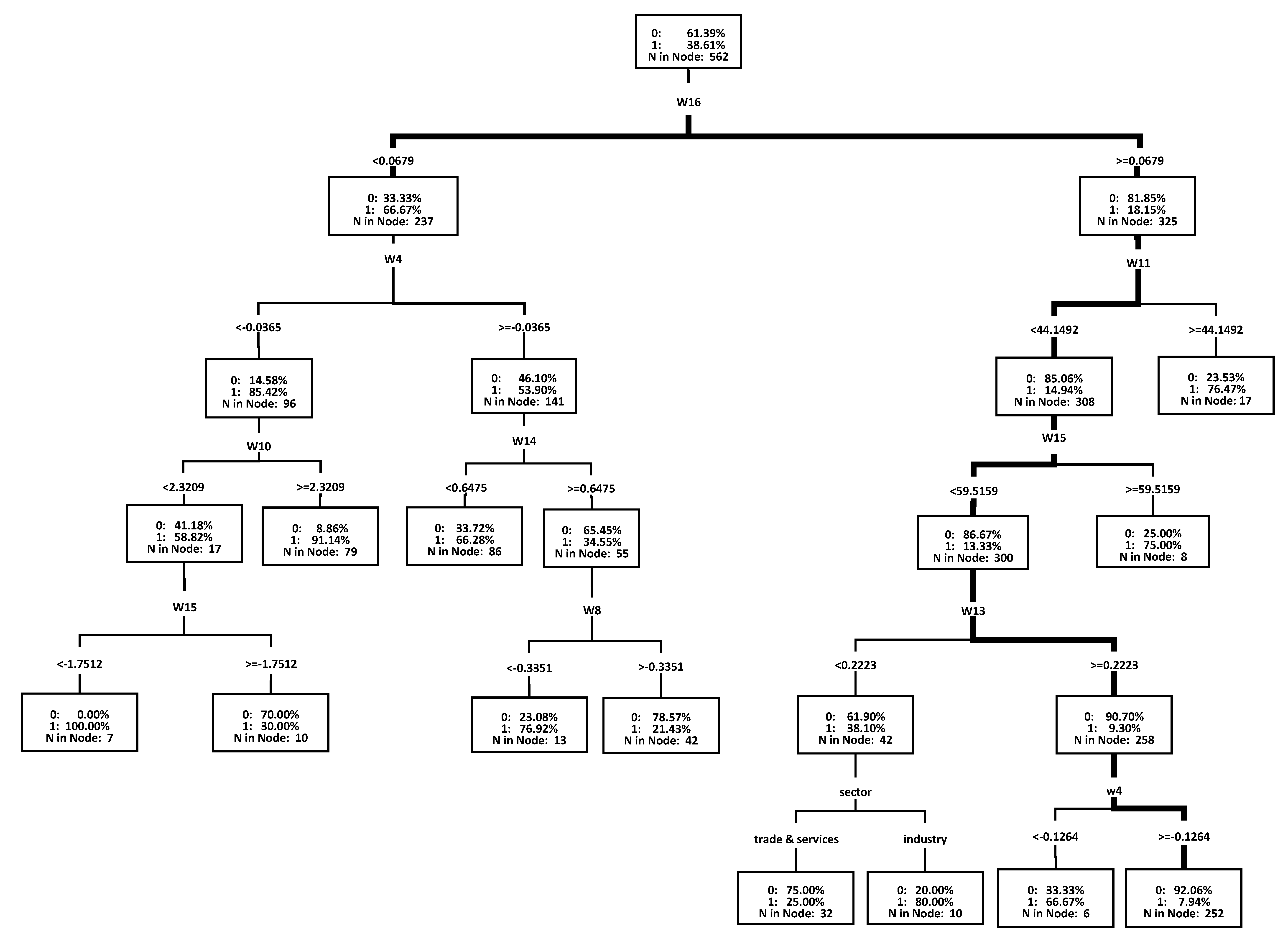
For decision tree the CART tree was used. For interval variables the splitting was based on F test and for nominal variables the chi-square test with a 0.2 p-value. A maximum of two subgroups in one split was allowed and maximum 6 splits in depth as the stopping criteria. Eight different financial ratios were used in splitting and two of them were used twice. Only one non-financial factor was used in splitting: sector (see Table 3). Results in graphical form are presented in Figure 4.
The first split was done according to ratio w16 into a group with almost a twice higher level of bankruptcy, w16 < 0.0679, and a group with almost twice lower level of bankruptcy, w16 ≥ 0.0679. Among those with w16 < 0.0679 there was a group with w4 < −0.0365 resulting in bankruptcy level 85.4% and further split according w10 < 2.32 giving the bankruptcy rate above 91% (more than 2.4 times higher comparing to total sample). The lowest risk of bankruptcy was characteristic for enterprises with w16 ≥ 0.0679, and w11 < 44.15 and w15 < 59.5 and w13 ≥ 0.22 and w4 ≥ −0.12. In this group the bankruptcy rate was about 7.9% (more than 4.75 times lower comparing to total sample).
3.4. Gradient Boosting
The fourth applied model was gradient boosting based on trees with split into two subgroups and a maximum depth of 2. Subtree was selected based on lowest misclassification rate. In gradient boosting similar financial ratios were important. Among non-financial factors employment was more important compared to other factors (see Table 4).
3.5. Neural Network
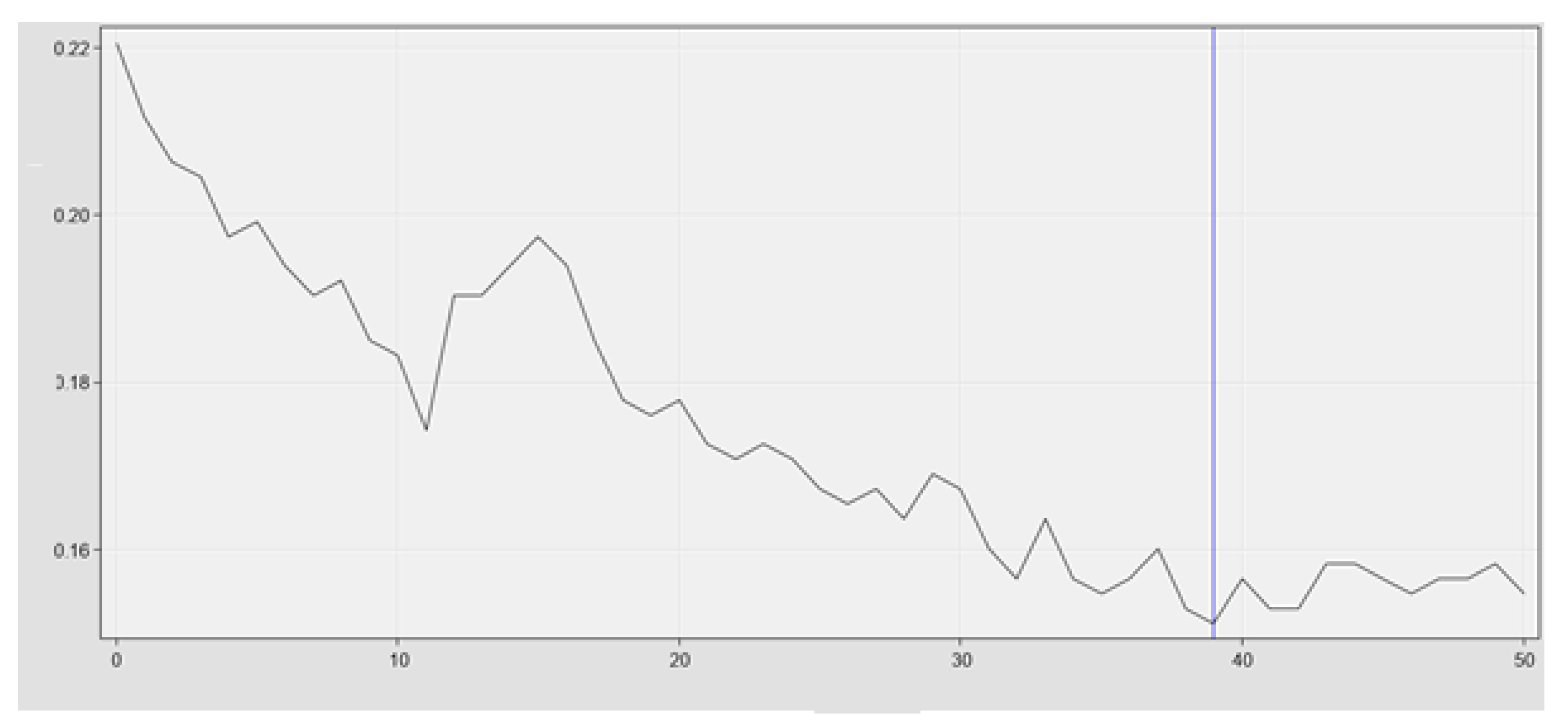
The most popular architecture of neural network was used the multi-layer perceptron (MLP) with one hidden layer. Number of neurons in the layer equals number of explanatory variables. pseudo-Newton optimization technique was used with maximum 200 iterations. A total of 106 parameters were estimated in total. The iteration history is shown in Figure 5.
3.6. Support Vectors Machine
As a final model, the SVM was estimated. As an optimization method the interior point was set with scaling and polynomial function (two degrees).
The penalization method was C with a penalization parameter equal 1. Maximum iterations was set to 25 with a tolerance 1 × 10⁻⁶. The results are presented in Table 5.
3.7. Model Comparison
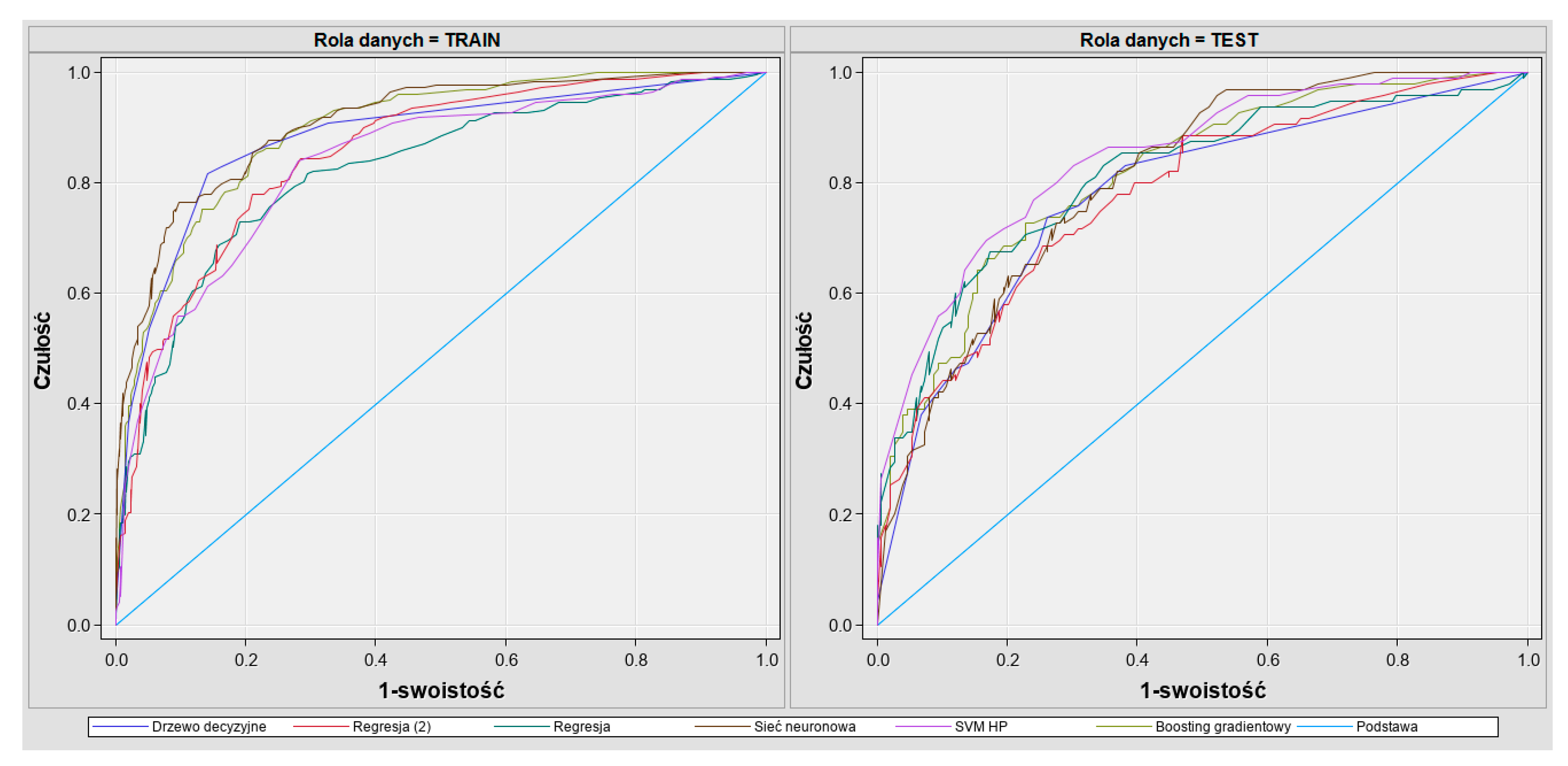
Model evaluation was based on the Gini (accuracy ratio—AR) coefficient on the test sample, which is a measure based on ROC, i.e., the curve used to measure the discriminative power of the model. It is applied in the case when the dependent variable is binary (it has two unique values). The Figure 6 presents the relation of the specificity to the sensitivity of the model. Both of those measures provide information on how effective the classification is in the context of both levels of the dependent variable. The ROC curve is a sensitivity function (on the vertical axis) and 1-specificity (on the horizontal axis). Each point of the curve corresponds to a given point of split (section). Points in the right upper corner correspond to a low q level. Points in the left bottom corner relate to a high q level. ROC does not depend on the assumed point of split. The rates are drawn for all points of split. While selecting a given point of split we can establish the specificity and sensitivity of the model for that point. Selecting a given point of split we can establish the number of successes and failures predicted by the model, and then calculate the sensitivity and the specificity of the model. The correspondent sensitivity and specificity levels are easy to read from the graph of the ROC curve. A good model has the ROC curve close to the upper-left boundary of the graph. Then we can find points on the curve representing high values both in terms of sensitivity and specificity (e.g., so that c > 0.8 and s > 0.8). The random model has the ROC curve lying on the diagonal. Then the sensitivity + specificity = 1 for all the threshold values of q. In such a case while establishing the value c > 0.8 we cannot ensure that the specificity is greater than 0.2. The ROC curve is helpful when selecting the optimal point of division. For example, we choose the threshold that gives equal probability of misclassification in each class. We also have to take into account the different cost of both types of misclassification and decide whether to provide high sensitivity or high specificity. The area under the ROC curve is a measure of the quality of the model. This way we can compare the quality of different models. The AUC (area under the ROC curve) for an ideal model equals 1 and for a random model 0.5.
The similar measure to ROC is the CAP curve, where the cumulative frequencies for good customers are substituted by frequencies for all customers. The area under the CAP curve is called the accuracy ratio. The CAP curve represents the y% of bankrupted enterprises that can be found in the x% of the worst assessed enterprises within the model. The curve should be concave. The accuracy ratio (Gini coefficient) based on the CAP curve is defined as:
where:
- BR—bankruptcy rate;
- —area under the CAP curve.
The value of AR is normalized in the range of [0; 1].
Comparing models Gini coefficient for test sample was used. The highest Gini coefficient for the test sample was reached by SVM and amounted at 0.69 (see Table 6). This model was not overfitted because Gini for the training sample was similar (0.67). Regression with interval ratios was also stable with similar results for train and test sample but slightly worse comparing to SVM. Neural network and decision tree models were overfitted because Gini was much higher for the training sample comparing to test sample. Gradient boosting had a high Gini for the test sample, but the difference for training and testing samples was too high. The shape of the ROC curve was correct for all models with the highest AUC for SVM (see Figure 3).
It is also important to compare the error rate for bankruptcy classifications and for non-bankruptcy classifications (see Table 7). Classification table was compared for the train sample (see Table 8). SVM with the highest Gini on the test sample had the highest rate of misclassification of bankruptcies (50%). Regression with interval ratios had lower rates of misclassifications of bankruptcies (44%). The decision tree with the lowest Gini coefficient for the test sample had the lowest misclassifications of bankruptcies (18%) for the training sample. The choice of the final model must be in equilibrium between accuracy and stability of the model (overfitting).
Taking into account different financial ratios and non-financial factors only six financial ratios and two non-financial factors were significant in at least two different models (see Table 9).
4. Discussion and Conclusions
Summing up above estimation we can conclude that simple models like logistic regression were as good as more complex models like neural networks (NN), decision trees (DT), or support vector machines (SVM). However, in other research, like Zięba et al. (2016), who applied the extreme gradient boosting model, results gained by the selected classifier were significantly better than the results gained by all other simpler methods that were applied by authors to the problem of predicting financial condition of the companies. In different classification analysis not only concerning financial ratios quite often SVM is stated as promising method (see Lahmiri et al. 2017; Lahmiri and Shmuel 2018).
Data mining models are less stable and tend to be overfitted (see Gradient Boosting, Neural Network, and Decision Tree sections). The difference of accuracy between train and test sample was too high.
Financial ratios that were most important in predicting small enterprise failures were: operating profitability of assets, current assets turnover, capital ratio, coverage of short-term liabilities by equity, coverage of fixed assets by equity, and share of net financial surplus in total liabilities. Results may be compared to results recently obtained for Polish bankruptcy data by Zięba et al. (2016). The authors examined data for Polish bankrupted companies from period 2007–2013. They analyzed a five-year period and only three indicators: adjusted share of equity in financing of assets, current ratio, liabilities turnover ratio appeared in each analyzed year. According to authors those ratios can be considered as useful in predicting bankruptcy of enterprises.
Among non-financial factors two of them were important: sector of activity and employment. The usage of non-financial ratios improves the results of all models which confirmed our expectations and other research. The legal form of the company seems to be the most important variable among all the considered non-financial factors. Employment and sector also plays a role, which confirms the results obtained by Chava and Jarrow (2004). Gordini (2014) confirmed that building models tailored to specific geographical areas increases the accuracy. However, in our models two variables, region and age of the company, seem to play a much less important role.
The hypotheses were positively verified:
Hypothesis 3 (H3):
Non-financial factors are important in case of predicting small enterprises success and failures.
Hypothesis 4 (H4):
More advanced and complicated models are not necessary to predict small enterprise failures. Simple models are as effective as more complex ones.
As always the greatest problem is the access to good quality data. Depending on the data availability future research would cover the interaction with the macroeconomic situation. Financial situations expanded by non-financial factors do not give the full view of the bankruptcy causes. Deeper analysis of causality mechanisms is needed.
Funding
This research received no external funding.
Conflicts of Interest
The authors declare no conflict of interest.
References
- Altman, Edward I. 1968. Financial ratios, Discriminant analysis and the prediction of corporate bankruptcy. Journal of Finance 23: 589–609. [Google Scholar] [CrossRef]
- Appenzeller, Dorota, and Katarzyna Szarzec. 2004. Forecasting the bankruptcy risk of Polish public companies. Rynek Terminowy 1: 120–28. [Google Scholar]
- Aziz, M. Adnan, and Humayon A. Dar. 2006. Predicting Corporate Bankruptcy: Where do We Stand? Corporate Governance International Journal of Business in Society 6: 18–33. [Google Scholar] [CrossRef]
- Back, Barbro, Teija Laitinen, Kaisa Sere, and Michiel van Wezel. 1996. Choosing Bankruptcy Predictors Using Discriminant Analysis, Logit Analysis, and Genetic Algorithms. Technical Report. Turku: Turku Centre for Computer Science. [Google Scholar]
- Balina, Rafał, and Maksymilian Jan Bąk. 2016. Discriminant Analysis as a Prediction Method for Corporate Bankruptcy with the Industrial Aspects. Waleńczów: Wydawnictwo Naukowe Intellect. [Google Scholar]
- Blanco-Oliver, Antonio, Rafael Pino-Mejías, Juan Lara-Rubio, and Salvador Rayo. 2013. Credit scoring models for the microfinance industry using neural networks: Evidence from Peru. Expert Systems with Applications 40: 356–64. [Google Scholar] [CrossRef]
- Brożyna, Jacek, Grzegorz Mentel, and Tomasz Pisula. 2016. Statistical methods of the bankruptcy prediction in the logistics sector in Poland and Slovakia. Transformations in Business & Economics 15: 80–96. [Google Scholar]
- Calabrese, Raffaella, Giampiero Marra, and Silvia Angela Osmetti. 2015. Bankruptcy prediction of small and medium enterprises using a flexible binary generalized extreme value model. Journal of the Operational Research Society 67: 604–15. [Google Scholar] [CrossRef]
- Chaudhuri, Arindam, and Kajal De. 2011. Fuzzy support vector machine for bankruptcy prediction. Applied Soft Computing 11: 2472–86. [Google Scholar] [CrossRef]
- Chava, Sudheer, and Robert A. Jarrow. 2004. Bankruptcy prediction with industry effects. Review of Finance 8: 537–569. [Google Scholar] [CrossRef]
- Gajdka, Jerzy, and Daniel Stos. 1996. The use of discriminant analysis in assessing the financial condition of enterprises. In Restructuring in the Process of Transformation and Development of Enterprises. Edited by Ryszard Borowiecki. Kraków: Wydawnictwo Akademii Ekonomicznej w Krakowie. [Google Scholar]
- Gąska, Damian. 2016. Predicting Bankruptcy of Enterprises with the use of Learning Methods. Ph.D. dissertation, Wrocław University of Economics, Wrocław, Poland. [Google Scholar]
- Gordini, Niccolo. 2014. A genetic algorithm approach for SMEs bankruptcy prediction: Empirical evidence from Italy. Expert Systems with Applications 41: 6067–536. [Google Scholar] [CrossRef]
- Gruszczyński, Marek. 2003. Models of Microeconometrics in the Analysis and Forecasting of the Financial Risk of Enterprises. Warszawa: Zeszyty Polskiej Akademii Nauk nr 23. [Google Scholar]
- Gupta, Jairaj, Andros Gregoriou, and Jerome Healy. 2015. Forecasting bankruptcy for SMEs using hazard function: A review of quantitative finance and accounting. Review of Quantitative Finance and Accounting 45: 845–69. [Google Scholar] [CrossRef]
- Hadasik, Dorota. 1998. The Bankruptcy of Enterprises in Poland and Methods of its Forecasting. Poznań: Wydawnictwo Akademii Ekonomicznej w Poznaniu, vol. 153. [Google Scholar]
- Hamrol, Mirosław, Bartłomiej Czajka, and Maciej Piechocki. 2004. Enterprise bankruptcy—discriminant analysis model. Przegląd Organizacji 6: 35–39. [Google Scholar]
- Hołda, Artur. 2001. Forecasting the bankruptcy of an enterprise in the conditions of the Polish economy using the discriminatory function ZH. Rachunkowość 5: 306–10. [Google Scholar]
- Jagiełło, Robert. 2013. Discriminant and Logistic Analysis in the Process of Assessing the Creditworthiness of Enterprises. Materiały i Studia, Zeszyt 286. Warszawa: NBP. [Google Scholar]
- Jiménez, Gabriel, and Jesus Saurina. 2004. Collateral, type of lender and relationship banking as determinants of credit risk. Journal of Banking & Finance 28: 2191–212. [Google Scholar]
- Kalak, El Izidin, and Robert Hudson. 2016. The effect of size on the failure probabilities of SMEs: An empirical study on the US market using discrete hazard model. International Review of Financial Analysis 43: 135–45. [Google Scholar] [CrossRef]
- Karbownik, Lidia. 2017. Methods for Assessing the Financial Risk of Enterprises in the TSI Sector in Poland. Łódź: Wydawnictwo Uniwersytetu Łódzkiego. [Google Scholar]
- Kim, Hong Sik, and So Young Sohn. 2010. Support Vector Machines for Default Prediction of SMEs Based on Technology Credit. European Journal of Operational Research 201: 838–46. [Google Scholar] [CrossRef]
- Korol, Tomasz. 2004. Assessment of the Accuracy of the Application of Discriminatory Methods and Artificial Neural Networks for the Identification of Enterprises Threatened with Bankruptcy. Doctoral dissertation, University of Gdańsk, Gdańsk, Poland. [Google Scholar]
- Korol, Tomasz. 2010a. Early Warning Systems of Enterprises to the Risk of Bankruptcy. Warszawa: Wolters Kluwer. [Google Scholar]
- Korol, Tomasz. 2010b. Forecasting bankruptcies of companies using soft computing techniques. Finansowy Kwartalnik Internetowy “e-Finanse” 6: 1–14. [Google Scholar]
- Lahmiri, Salim. 2016a. Features selection, data mining and financial risk classification: A comparative study. Intelligent Systems in Accounting. Finance and Management 23: 265–75. [Google Scholar]
- Lahmiri, Salim. 2016b. On simulation performance of feedforward and NARX networks under different numerical training algorithms. In Handbook of Research on Computational Simulation and Modeling in Engineering. Hershey: IGI. [Google Scholar]
- Lahmiri, Salim. 2016c. Prediction of International Stock Markets Based on Hybrid Intelligent Systems. In Handbook of Research on Innovations in Information Retrieval, Analysis, and Management. Hershey: IGI. [Google Scholar]
- Lahmiri, Salim. 2017. A two-step system for direct bank telemarketing outcome classification. Intelligent Systems in Accounting. Finance and Management 24: 49–55. [Google Scholar]
- Lahmiri, Salim, Debra Ann Dawson, and Amir Smuel. 2017. Performance of machine learning methods in diagnosing Parkinson’s disease based on dysphonia measures. Biomedical Engineering Letters 8: 1–11. [Google Scholar] [CrossRef] [PubMed]
- Lahmiri, Salim, and Amir Shmuel. 2018. Performance of machine learning methods applied to structural MRI and ADAS cognitive scores in diagnosing Alzheimer’s disease. Biomedical Signal Processing and Control. [Google Scholar] [CrossRef]
- Mączyńska, Elżbieta. 1994. Assessment of the condition of the enterprise. Simplified methods. Życie Gospodarcze 38: 42–45. [Google Scholar]
- Mączyńska, Elżbieta. 2004. Early warning systems. Nowe Życie Gospodarcze 12: 4–9. [Google Scholar]
- Michaluk, Krzysztof. 2003. Effectiveness of corporate bankruptcy models in Polish economic conditions. In Corporate Finance in the Face of Globalization Processes. Edited by Leszek Pawłowicz and Ryszard Wierzba. Warszawa: Wydawnictwo Gdańskiej Akademii Bankowej. [Google Scholar]
- Ong, Chorng-Shyong, Jih-Jeng Huang, and Gwo-Hshiung Tzeng. 2005. Building credit scoring models using genetic programming. Expert Systems with Applications 29: 41–47. [Google Scholar] [CrossRef]
- Pociecha, Józef, and Barbara Pawełek. 2011. Bankruptcy Prediction and Business Cycle, Contemporary Problems of Transformation Process in the Central and East European Countries. Paper presented at 17th Ukrainian-Polish-Slovak Scientific Seminar, Lviv, Ukraine, September 22–24; Lviv: The Lviv Academy of Commerce, pp. 9–24. [Google Scholar]
- Pociecha, Józef, Barbara Pawełek, Mateusz Baryła, and Sabina Augustyn. 2014. Statistical Methods of Forecasting Bankruptcy in the Changing Economic Situation. Kraków: Fundacja Uniwersytetu Ekonomicznego w Krakowie. [Google Scholar]
- Pogodzińska, Marzanna, and Sławomir Sojak. 1995. The Use of Discriminant Analysis in Predicting Bankruptcy of Enterprises. Ekonomia XXV, Zeszyt 299. Toruń: AUNC. [Google Scholar]
- Prusak, Błażej. 2018. Review of Research into Enterprise Bankruptcy Prediction in Selected Central and Eastern European Countries. International Journal of Financial Studies 6: 60. [Google Scholar] [CrossRef]
- Prusak, Błażej, and Agnieszka Więckowska. 2007. Multidimensional models of discriminant analysis in the study of the bankruptcy risk of Polish companies listed on the WSE. In Economic and Legal Aspects of Corporate Bankruptcy. Edited by Błażej Prusak. Warszawa: Difin. [Google Scholar]
- Prusak, Błażej. 2005. Modern Methods of Forecasting Financial Risk of Enterprises. Warszawa: Difin. [Google Scholar]
- Psillaki, Maria, Ioannis E. Tsolas, and Dimitris Margaritis. 2010. Evaluation of credit risk based on firm performance. European Journal of Operational Research 201: 873–81. [Google Scholar] [CrossRef]
- Ptak-Chmielewska, Aneta, and Anna Matuszyk. 2017. The importance of financial and non-financial ratios in SMEs bankruptcy prediction. Bank i Kredyt 49: 45–62. [Google Scholar]
- Ptak-Chmielewska, Aneta. 2016. Statistical Models for Corporate Credit Risk Assessment—Rating Models. Acta Universitatis Lodziensis Folia Oeconomica 3: 98–111. [Google Scholar] [CrossRef]
- Sartori, Fabio, Alice Mazzucchelli, and Angelo Di Gregorio. 2016. Bankruptcy forecasting using case-based reasoning: The CRePERIE approach. Expert Systems with Applications 64: 400–11. [Google Scholar] [CrossRef]
- Sohn, So Young, Dong Ha Kim, and Jin Hee Yoon. 2016. Technology credit scoring model with fuzzy logistic regression. Applied Soft Computing 43: 150–58. [Google Scholar] [CrossRef]
- Sojak, Sławomir, and Józef Stawicki. 2000. The use of taxonomic methods to assess the economic condition of enterprises. Zeszyty Teoretyczne Rachunkowości 3: 55–66. [Google Scholar]
- Stępień, Paweł, and Tomasz Strąk. 2003. Signs of the threat of bankruptcy of Polish enterprises—Empirical study. In Time for Money, t. II. Edited by Dariusz Zarzecki. Szczecin: Wydawnictwo Uniwersytetu Szczecińskiego. [Google Scholar]
- Stępień, Paweł, and Tomasz Strąk. 2004. Multidimensional logit models for assessing the risk of bankruptcy of Polish enterprises. In Time for Money, t. I. Edited by Dariusz Zarzecki. Szczecin: Wydawnictwo Uniwersytetu Szczecińskiego. [Google Scholar]
- Wędzki, Dariusz. 2000. The problem of using the ratio analysis to predict the bankruptcy of Polish enterprises—Case study. Bank i Kredyt 5: 54–61. [Google Scholar]
- Wędzki, Dariusz. 2004. Logit model of bankruptcy for the Polish economy—Conclusions from the study. In Time for Money. Corporate Finance. Financing Enterprises in the EU. Edited by Dariusz Zarzecki. Szczecin: Wydawnictwo Uniwersytetu Szczecińskiego. [Google Scholar]
- Wierzba, Dariusz. 2000. Early Detection of Enterprises Threatened with Bankruptcy Based on the Analysis of Financial Ratios—Theory and Empirical Research. Zeszyty Naukowe nr 9. Warszawa: Wydawnictwo Wyższej Szkoły Ekonomiczno-Informatycznej w Warszawie. [Google Scholar]
- Zięba, Maciej, Sebastian K. Tomczak, and Jakub M. Tomczak. 2016. Ensemble boosted trees with synthetic features generation in application to bankruptcy prediction. Expert Systems with Applications 58: 93–101. [Google Scholar] [CrossRef]
- Zmijewski, Me. 1984. Methodological issues related to the estimation of financial distress prediction models. Journal of Accounting Research 22: 59–82. [Google Scholar] [CrossRef]
Figure 1.
Decision tree—graphical representation.

Figure 2.
Neural network model.

Figure 3.
SVM mechanism. (a) Optimal classification; (b) mapping.

Figure 4.
Results of the estimation of the decision tree.

Figure 5.
Neural network—iterations history (misclassification rate—training sample).

Figure 6.
ROC curve for all models, train and test sample.


Table 1.
Results of estimation of logistic regression with interval variables.
| Variable | DF | Parameter | Std Err | Wald Chi-sqr | p-Value | Exp(x) |
|---|---|---|---|---|---|---|
| Intercept | 1 | −1.0053 | 0.3845 | 6.83 | 0.0089 | 0.366 |
| legal_form 2 | 1 | 0.4244 | 0.3065 | 1.92 | 0.1661 | 1.529 |
| legal_form 3 | 1 | −0.7052 | 0.4612 | 2.34 | 0.1262 | 0.494 |
| legal_form 4 | 0 | 0 | . | . | . | . |
| Sector 1 | 1 | 0.4922 | 0.2631 | 3.50 | 0.0613 | 1.636 |
| Sector 2 | 1 | 0.8228 | 0.2609 | 9.95 | 0.0016 | 2.277 |
| Sector 3 | 0 | 0 | . | . | . | . |
| w1 | 1 | 0.0893 | 0.0323 | 7.64 | 0.0057 | 1.093 |
| w10 | 1 | 0.1426 | 0.0335 | 18.09 | <0.0001 | 1.153 |
| w13 | 1 | −2.8207 | 0.4264 | 43.75 | <0.0001 | 0.060 |
| w7 | 1 | −2.1131 | 0.5771 | 13.41 | 0.0003 | 0.121 |
Table 2.
Results of estimation of logistic regression with discretized variables.
| Variable | DF | Parameter | Std Err | Wald Chi-sqr | p-Value | Exp(x) |
|---|---|---|---|---|---|---|
| Intercept | 1 | −0.9796 | 0.4283 | 5.23 | 0.0222 | 0.375 |
| GRP_employment 1 | 1 | 0.8388 | 0.3806 | 4.86 | 0.0275 | 2.314 |
| GRP_employment 2 | 1 | 0.0969 | 0.3413 | 0.08 | 0.7765 | 1.102 |
| GRP_employment 3 | 1 | 0.1829 | 0.3726 | 0.24 | 0.6235 | 1.201 |
| GRP_employment 4 | 1 | 0.8616 | 0.3454 | 6.22 | 0.0126 | 2.367 |
| GRP_employment 5 | 0 | 0 | . | . | . | . |
| GRP_w11 1 | 1 | −1.2379 | 0.3450 | 12.87 | 0.0003 | 0.290 |
| GRP_w11 2 | 1 | −1.4883 | 0.3486 | 18.23 | <0.0001 | 0.226 |
| GRP_w11 3 | 1 | −1.6453 | 0.3540 | 21.60 | <0.0001 | 0.193 |
| GRP_w11 4 | 1 | −1.7106 | 0.3587 | 22.74 | <0.0001 | 0.181 |
| GRP_w11 5 | 0 | 0 | . | . | . | . |
| GRP_w13 1 | 1 | 1.3206 | 0.4528 | 8.51 | 0.0035 | 3.746 |
| GRP_w13 2 | 1 | 1.2484 | 0.4367 | 8.17 | 0.0043 | 3.485 |
| GRP_w13 3 | 1 | 0.2725 | 0.4296 | 0.40 | 0.5258 | 1.313 |
| GRP_w13 4 | 1 | −0.5903 | 0.4334 | 1.85 | 0.1732 | 0.554 |
| GRP_w13 5 | 0 | 0 | . | . | . | . |
| GRP_w16 1 | 1 | 2.4878 | 0.4438 | 31.42 | <0.0001 | 12.034 |
| GRP_w16 2 | 1 | 1.1336 | 0.4505 | 6.33 | 0.0119 | 3.107 |
| GRP_w16 3 | 1 | 0.2847 | 0.4624 | 0.38 | 0.5381 | 1.329 |
| GRP_w16 4 | 1 | −0.3871 | 0.4548 | 0.72 | 0.3947 | 0.679 |
| GRP_w16 5 | 0 | 0 | . | . | . | . |
Table 3.
Importance of variables in the decision tree.
| Variable | Number of Rules | Importance |
|---|---|---|
| w16 | 1 | 1.0000 |
| w4 | 2 | 0.4884 |
| w11 | 1 | 0.4349 |
| w15 | 2 | 0.3930 |
| w14 | 1 | 0.3236 |
| w8 | 1 | 0.3079 |
| w13 | 1 | 0.3047 |
| sector | 1 | 0.2673 |
| w10 | 1 | 0.2128 |
Table 4.
Importance of variables in the decision tree.
| Variable | Number of Rules | Importance |
|---|---|---|
| w16 | 16 | 1.00000 |
| w13 | 6 | 0.60837 |
| w11 | 14 | 0.60156 |
| w15 | 5 | 0.40503 |
| employment | 11 | 0.38090 |
| w14 | 7 | 0.33149 |
| w7 | 4 | 0.32444 |
| w5 | 6 | 0.31146 |
| w6 | 6 | 0.30114 |
| w1 | 4 | 0.28198 |
| w3 | 6 | 0.27084 |
| age | 4 | 0.24969 |
| w12 | 5 | 0.23794 |
| w2 | 5 | 0.23771 |
| w10 | 5 | 0.20920 |
| sector | 3 | 0.19020 |
| legal_form | 3 | 0.18527 |
| w4 | 2 | 0.16845 |
| w8 | 3 | 0.15562 |
| w9 | 2 | 0.12812 |
| region_cluster | 2 | 0.12418 |
Table 5.
Results of SVM training.
| Internal product of weights | 46.3039131 |
| Burden | –21.744579 |
| Total stock (violation of restrictions) | 305.767624 |
| Norm of the longest vector | 11.6448785 |
| Number of support vectors | 387 |
| Number of support vectors on margin | 334 |
| Maximal F | 2.84554647 |
| Minimal F | –21.760742 |
| Number of effects | 21 |
| Columns of data matrix | 36 |
| Columns of kernel matrix | 703 |
Table 6.
Comparison of models based on test and train sample.
| Model | Test | Train | Train | Train | Train |
|---|---|---|---|---|---|
| Gini | MSE | MSC | ROC | Gini | |
| SVM | 0.690 | 0.19078 | 0.23665 | 0.835 | 0.671 |
| Boost | 0.632 | 0.12880 | 0.18327 | 0.895 | 0.791 |
| Reg1 | 0.622 | 0.16336 | 0.23665 | 0.823 | 0.647 |
| Neural | 0.612 | 0.11745 | 0.15125 | 0.907 | 0.814 |
| Reg2 | 0.554 | 0.14974 | 0.23310 | 0.854 | 0.708 |
| Tree | 0.552 | 0.12275 | 0.15836 | 0.881 | 0.762 |
Table 7.
Classification table.
| Model = 0 | Model = 1 | ||
|---|---|---|---|
| Level = 0 | TP | FP | OP |
| Level = 1 | FN | TN | ON |
| PP | PN | Total |
TP—true positive, FP—false positive, FN—false negative, TN—true negative, PP—predicted positive, PN—predicted negative, OP—original positive, ON—original negative.
Table 8.
Classification table—training sample.
| Model | FN | TP | FP | TN | % (FN/ON) |
|---|---|---|---|---|---|
| SVM | 108 | 320 | 25 | 109 | 50% |
| Boost | 65 | 307 | 38 | 152 | 30% |
| Reg1 | 96 | 308 | 37 | 121 | 44% |
| Neural | 51 | 311 | 34 | 166 | 24% |
| Reg2 | 78 | 292 | 53 | 139 | 36% |
| Tree | 40 | 296 | 49 | 177 | 18% |
Table 9.
Financial ratios and non-financial factors—significance in different models.
| Model | x1 | x2 | x3 | x4 | x5 | x6 | x7 | x8 | x9 | x10 | x11 | x12 | x13 | x14 | x15 | x16 |
|---|---|---|---|---|---|---|---|---|---|---|---|---|---|---|---|---|
| SVM | ||||||||||||||||
| Boost | x | x | x | x | x | x | x | |||||||||
| Reg1 | x | x | x | x | ||||||||||||
| Neural | ||||||||||||||||
| Reg2 | x | x | x | |||||||||||||
| Tree | x | x | x | x | x | x | x | x |
| Model | Legal Form | Sector | Age | Region | Employment |
|---|---|---|---|---|---|
| SVM | |||||
| Boost | x | ||||
| Reg1 | x | x | |||
| Neural | |||||
| Reg2 | x | ||||
| Tree | x |
© 2019 by the author. Licensee MDPI, Basel, Switzerland. This article is an open access article distributed under the terms and conditions of the Creative Commons Attribution (CC BY) license (http://creativecommons.org/licenses/by/4.0/).
Share and Cite
MDPI and ACS Style
Ptak-Chmielewska, A. Predicting Micro-Enterprise Failures Using Data Mining Techniques. J. Risk Financial Manag. 2019, 12, 30. https://doi.org/10.3390/jrfm12010030
AMA Style
Ptak-Chmielewska A. Predicting Micro-Enterprise Failures Using Data Mining Techniques. Journal of Risk and Financial Management. 2019; 12(1):30. https://doi.org/10.3390/jrfm12010030
Chicago/Turabian StylePtak-Chmielewska, Aneta. 2019. "Predicting Micro-Enterprise Failures Using Data Mining Techniques" Journal of Risk and Financial Management 12, no. 1: 30. https://doi.org/10.3390/jrfm12010030