1. Introduction
The generation and progression of tropical storms over oceanic and shelf waters are associated with complicated and extreme responses in the upper ocean, including large surface waves, substantial surface cooling, intense turbulent mixing, and post-storm inertial and sub-inertial motions that significantly modulate the physical and biogeochemical properties of the upper water column for several days to weeks [
1,
2,
3,
4,
5,
6]. Among these catastrophic effects, vertical mixing is associated with several crucial impacts on the upper ocean. First, vertical mixing entrains atmospheric oxygen into the water column and re-oxygenates the mixed layer, thereby enhancing biological processes in the upper ocean [
7,
8,
9,
10]. Second, the intense cyclone winds cause upwelling that, along with the mixing across the water column, upwell the nutrient-rich water beneath the euphotic zone to the surface, significantly enhancing primary production by causing phytoplankton blooms in the aftermath of the cyclone [
11,
12,
13]. A third important impact of upper ocean mixing during tropical cyclones is the substantial effect on ocean currents from the surface to the base of the mixed layer. This imposes an additional challenge for 3D numerical ocean circulation models to accurately parameterize vertical mixing for the simulation of ocean currents [
14,
15,
16].
Many studies have addressed the dynamics of upper ocean mixing and surface cooling during and after tropical cyclones using field data, satellite observations, or numerical models (e.g., [
1,
17,
18,
19,
20,
21]). These studies showed that phenomena associated with the response of the upper ocean to a moving cyclone can be classified into two categories: the forcing stage and the relaxation stage responses. The forcing stage responses are caused by the direct effect of the cyclone’s intense winds causing high shear across the water column, deepening of the mixed layer, intense surface cooling, and substantial upwelling beneath the cyclone core. The relaxation stage starts right after the dissipation of the cyclone’s wind and includes the barotropic sub-inertial waves and baroclinic near-inertial oscillations indicating a sub-inertial wave with a period of several days to weeks [
22,
23]. During the forcing stage, surface cooling along the cyclone’s track and the mixed layer deepening across the water column are the most prominent oceanic responses [
18]. Under the cyclone’s core, the main contributors in producing these responses are vertical mixing, advection (upwelling), and air-sea heat exchange [
24]. The heat balance analysis of the mixed layer during different tropical cyclones showed that 75–90% of the mixed layer cooling was attributed to the vertical mixing, while 5–15% was attributed to upwelling and a little was due to air-sea heat exchange [
21,
25].
One prominent response of the sea surface to a cyclone is the asymmetric spatial pattern of surface cooling and mixing on the right and left sides of the cyclone. In the northern hemisphere, the largest surface cooling and mixed layer deepening are produced on the right front side of the cyclone due to the rightward bias resulting from the wind vector resonance with inertial currents. However, the location of maximum response may also change depending on pre-existing warm or cold core eddies in the proximity of the cyclone’s track [
24].
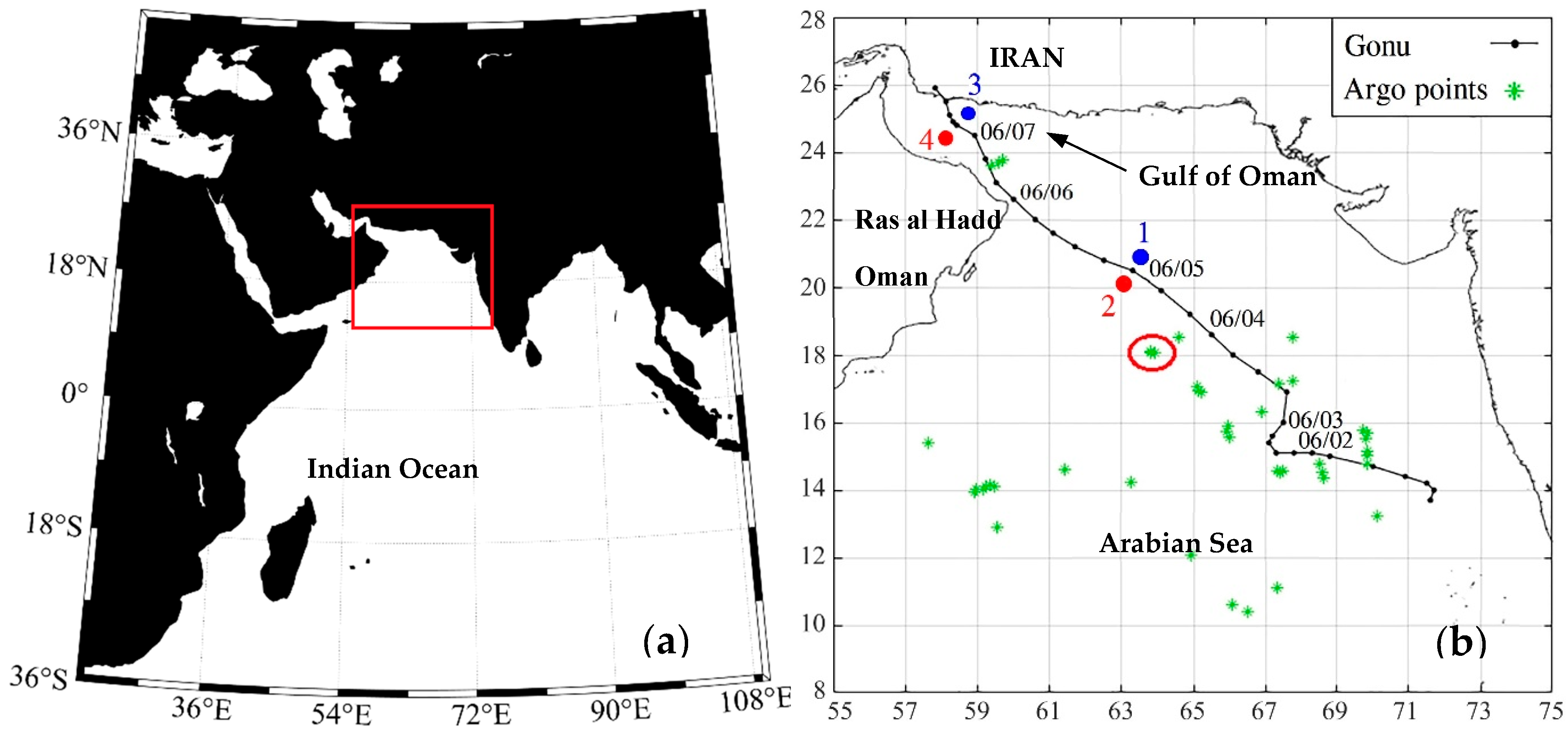
The northern Indian Ocean’s tropical cyclones rarely enter the northern Arabian Sea (NAS) or penetrate further north into the Gulf of Oman (see
Figure 1 for locations). By examining the best track data from the Joint Typhoon Warning Center (JTWC) and the Indian Meteorological Department for the period between 1877 and 2007, Dibajnia et al. [
26] suggested that only less than six tropical storms had made landfall on the coast of the NAS and Gulf of Oman. Hence, the studies that address oceanic response to a tropical cyclone in these basins are rare. Koohestani et al. [
23] studied the low-frequency oscillations and Kelvin-type surges produced in the wake of tropical storm Ashoobaa that made landfall on the southern coast of Oman in the NAS in June 2015. One of the most recent major tropical cyclones that entered the NAS is Gonu (2007), with a maximum intensity equivalent to a category 5 hurricane that made landfall on the Iranian coast in the northern Gulf of Oman. The surface wave response to this historical cyclone and its generated storm surge along the northern coast of the Gulf of Oman were studied by Allahdadi et al. [
5] and Allahdadi et al. [
27], respectively. Wang et al. [
28] used an array of deep- and shallow-water moorings to investigate the oscillatory response of the region to Gonu. They found that the forced oceanic response at most near-track stations was dominant. Although they reported salinity and temperature changes in the Gulf of Oman in the aftermath of Gonu as a result of Persian Gulf water intrusion, no specific investigations on the cyclone’s induced mixing were done. Upper ocean response to cyclones and especially the characteristic of induced mixing by cyclones in this region have less been studied. In fact, by the author’s knowledge, studies on the oceanic response to cyclones in this region are rare. Implementing such studies for this region is especially imperative due to its unique met-ocean (meteorological and oceanographic) conditions like the seasonal monsoon pattern and intense coastal upwelling along the Omani coast of the NAS [
29] that can interact with cyclone-induced mixing and alter the biogeochemical processes in the region.
This paper is one of the first attempts to study and quantify the upper ocean response, including surface cooling and mixed layer deepening, to a major cyclone in the NAS and Gulf of Oman with a focus on Cyclone Gonu. This study employs various types of data including satellite sea surface temperature (SST), climatological profiles of temperature, and Argo temperature/salinity profiler data for quantification of mixing, which is unprecedented for this region during a major tropical cyclone. The methodology used for estimation of the MLD based on satellite data is an effective, fast way for determining the MLD. The unique aspect of using this approach is that the quality of quantification was assessed based on the quality of input profiles and spatial variations of SST over the study area. This is another aspect of this paper that could set a precedent for future use of this approach for other regions and tropical cyclones.
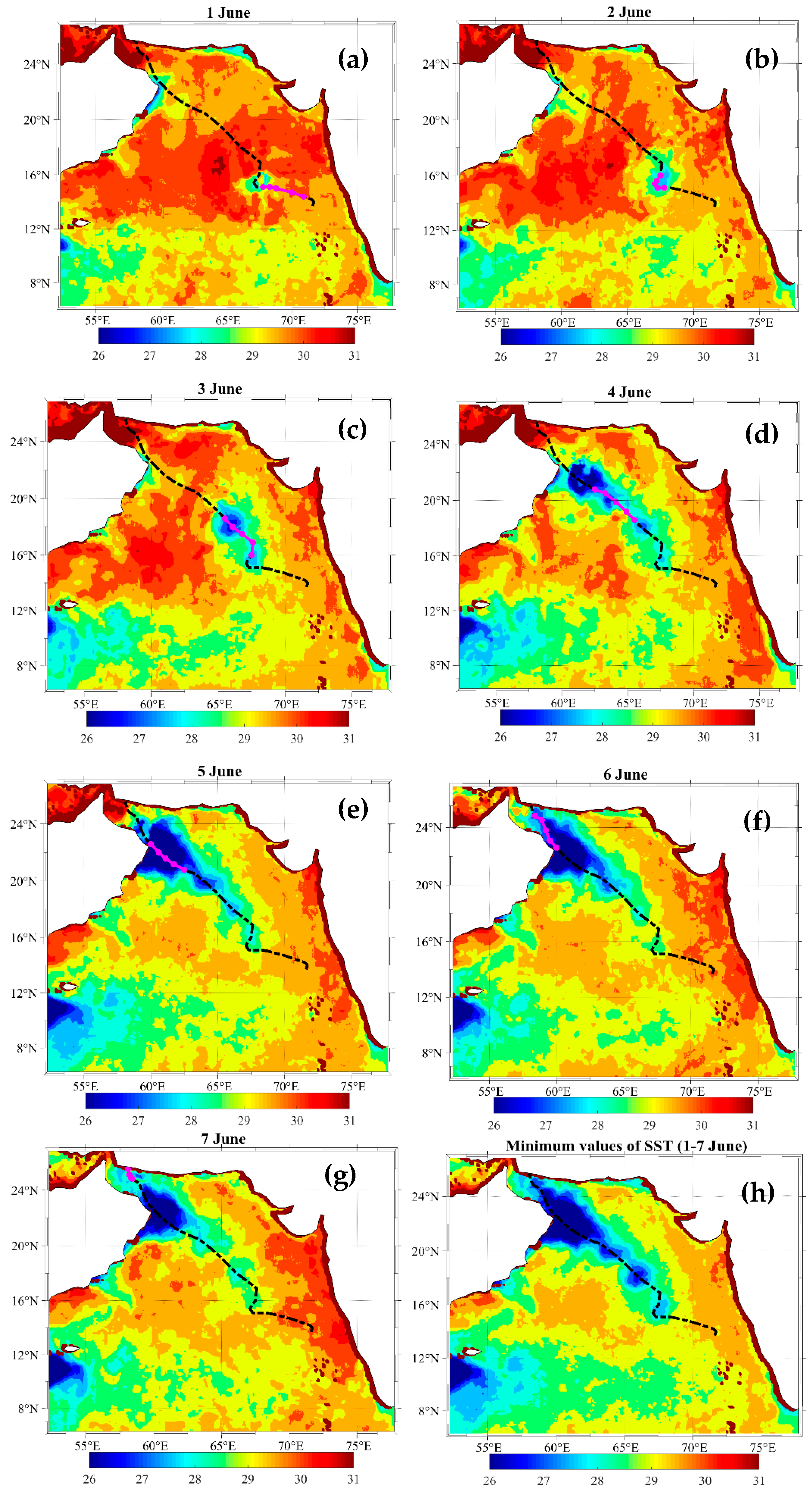
4. SST Response to Gonu
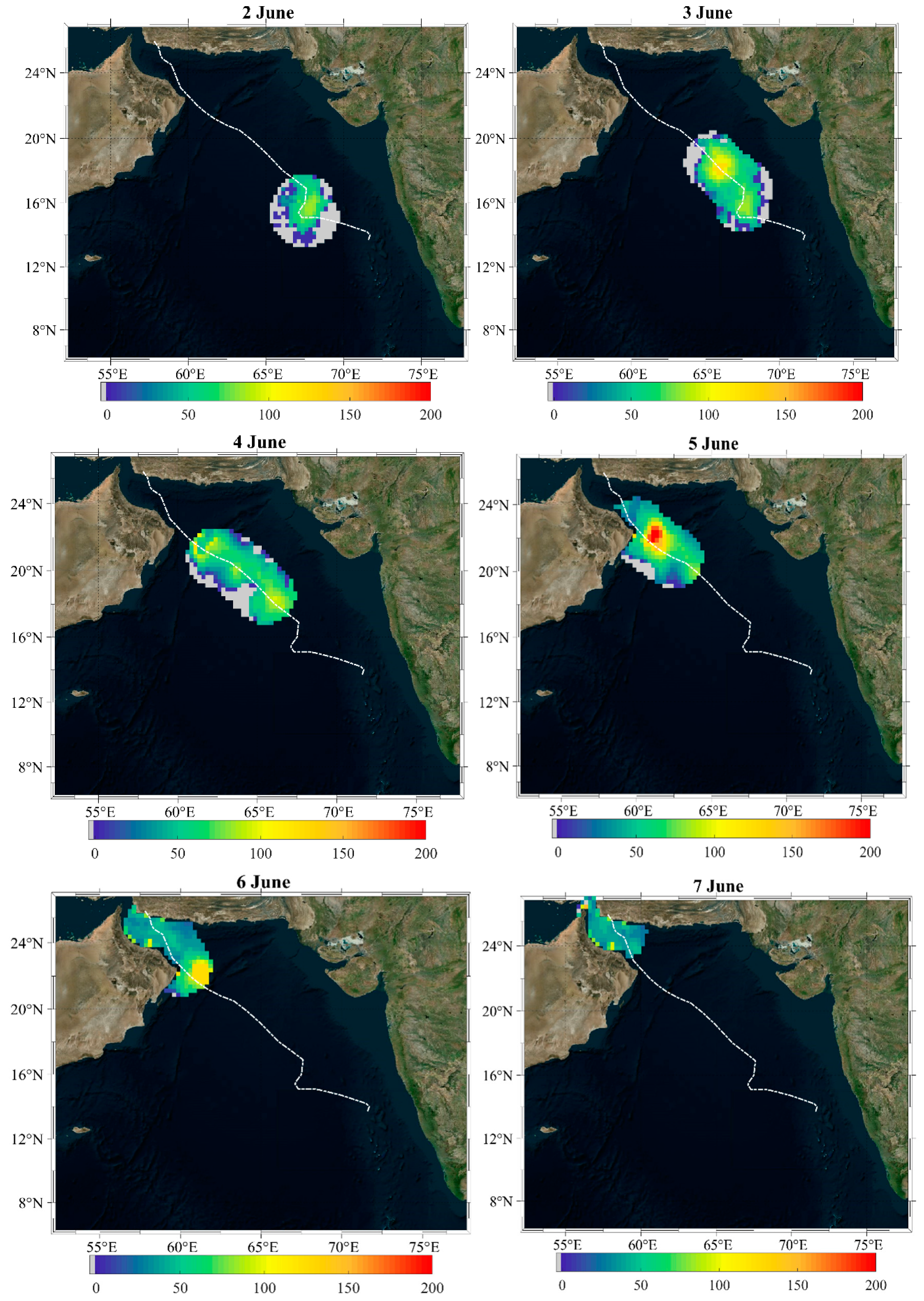
Redistribution of the upper ocean heat content by a cyclone changes the mixed layer temperature. At the sea surface, this redistribution can easily be detected from satellite-measured SST. The SST maps from the OI_SST database showing the effect of Cyclone Gonu on sea surface cooling in the NAS and Gulf of Oman from 1–7 June are presented in
Figure 2. Based on the satellite SST maps for 31 May 2007 (not shown), the day before Gonu formed, the average pre-cyclone SST over the NAS (latitude 12°–21° N) was about 30.5 °C. North of 21° N, the pre-cyclone SST was generally smaller (29.5–30 °C) except for the eastern Gulf of Oman for which the pre-cyclone SST was 31 °C or larger. Along the Oman coast, SST was as low as 27–27.5 °C due to the effect of summertime upwelling in this region [
29]. Maximum cyclone-induced SST cooling over the region on 1 and 2 June was 2.85 °C and 2.25 °C, respectively. Gonu was a tropical depression on 1 June and a category 1 tropical cyclone on 2 June. As the cyclone intensified during the following days, larger values for maximum SST cooling were observed. The cooling substantially increased as Gonu approached Ras al Hadd on the coast of Oman. The largest SST cooling during the time that Gonu was active in the study region (1–7 June) was 6.5 °C, observed on 4 June in the offshore region southeast of Ras al Hadd. On this date, the cyclone reached its highest strength (as strong as a category 5 hurricane). Although the cyclone’s intensity started to degrade on 5 June, the observed 5.5 °C cooling off the coast of Oman was still remarkable. By the time of landfall on 7 June, the maximum SST cooling decreased to 1.6 °C, which corresponded to degradation of the tropical cyclone to a tropical depression.
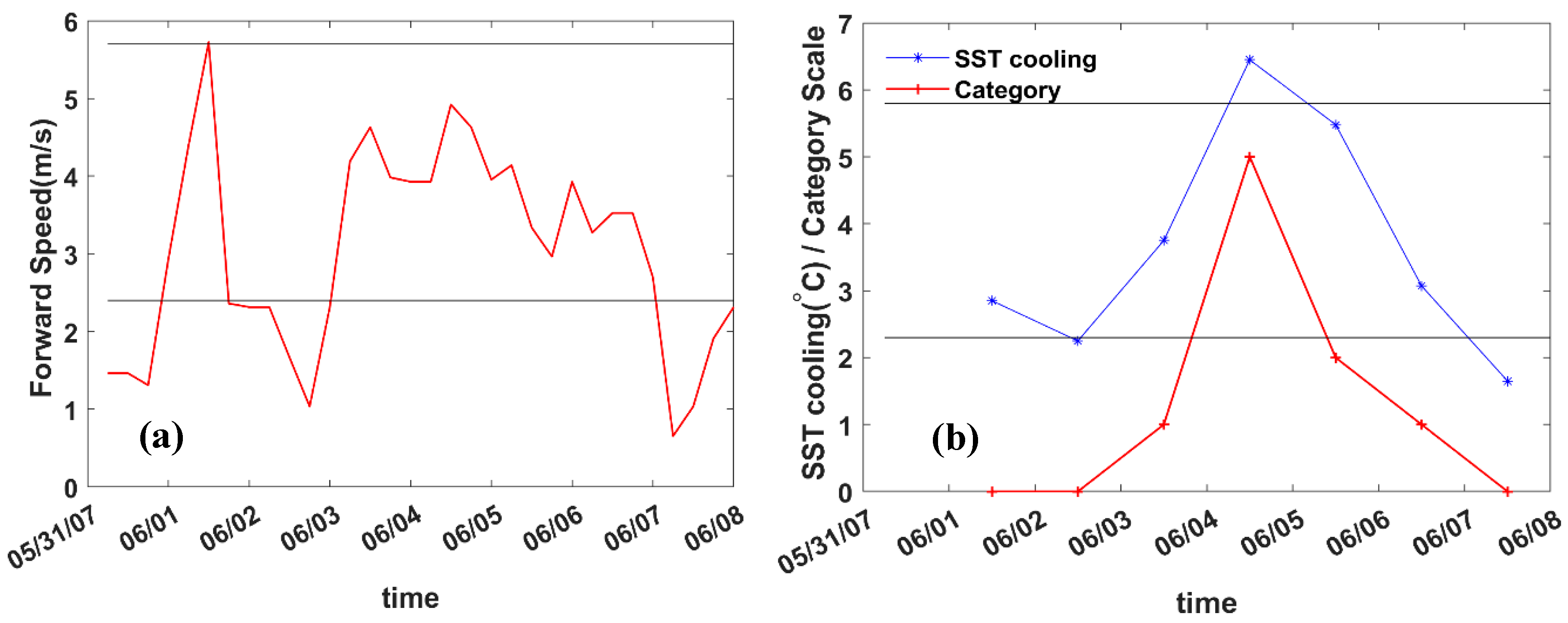
Both cyclone’s forward speed and intensity contributed to the magnitude of sea surface cooling. Bender et al. [
1] classified hurricanes (cyclones) into three categories based on their forward speed of slow- (2.4 m/s), medium- (5.7 m/s), and fast- (12 m/s) moving. They correspond to maximum average surface cooling of 5.8 °C, 2.3 °C, and 1.8 °C, respectively. Timeseries of forward speed for Cyclone Gonu (
Figure 3a) show that during the time that the cyclone translated the study area, its forward speed was between 1 and 6 m/s. For the strengthening phase of the cyclone (3–5 June), forward speeds were 2.5–5 m/s, making the cyclone a slow- to medium-moving storm. Thus, based on the above criterion of forward speed, the maximum SST cooling during 3–5 June should have been 2.3–5.8 °C. Timeseries of the maximum SST cooling over the study region (
Figure 3b) show that this is generally true. However, this classification cannot justify the most intense cooling that occurred on 4 June. This intense cooling can be attributed to the high intensity of Gonu’s category 5 hurricane-strength wind on 4 June (see
Figure 3b for timeseries of Gonu’s intensity).
Larger values of SST cooling (and broader cooling areas) in daily SST maps are mostly seen on the right side of the track. (
Figure 2a–g). This is due to the well-documented rightward bias phenomenon. In the northern hemisphere, the time variations of the wind stress vector on the right side of the cyclone’s track are clockwise [
1]. Therefore, the wind-induced currents (with the clockwise time variations) on the right front side of the cyclone are intensified by resonance with the inertial currents within the mixed layer [
1,
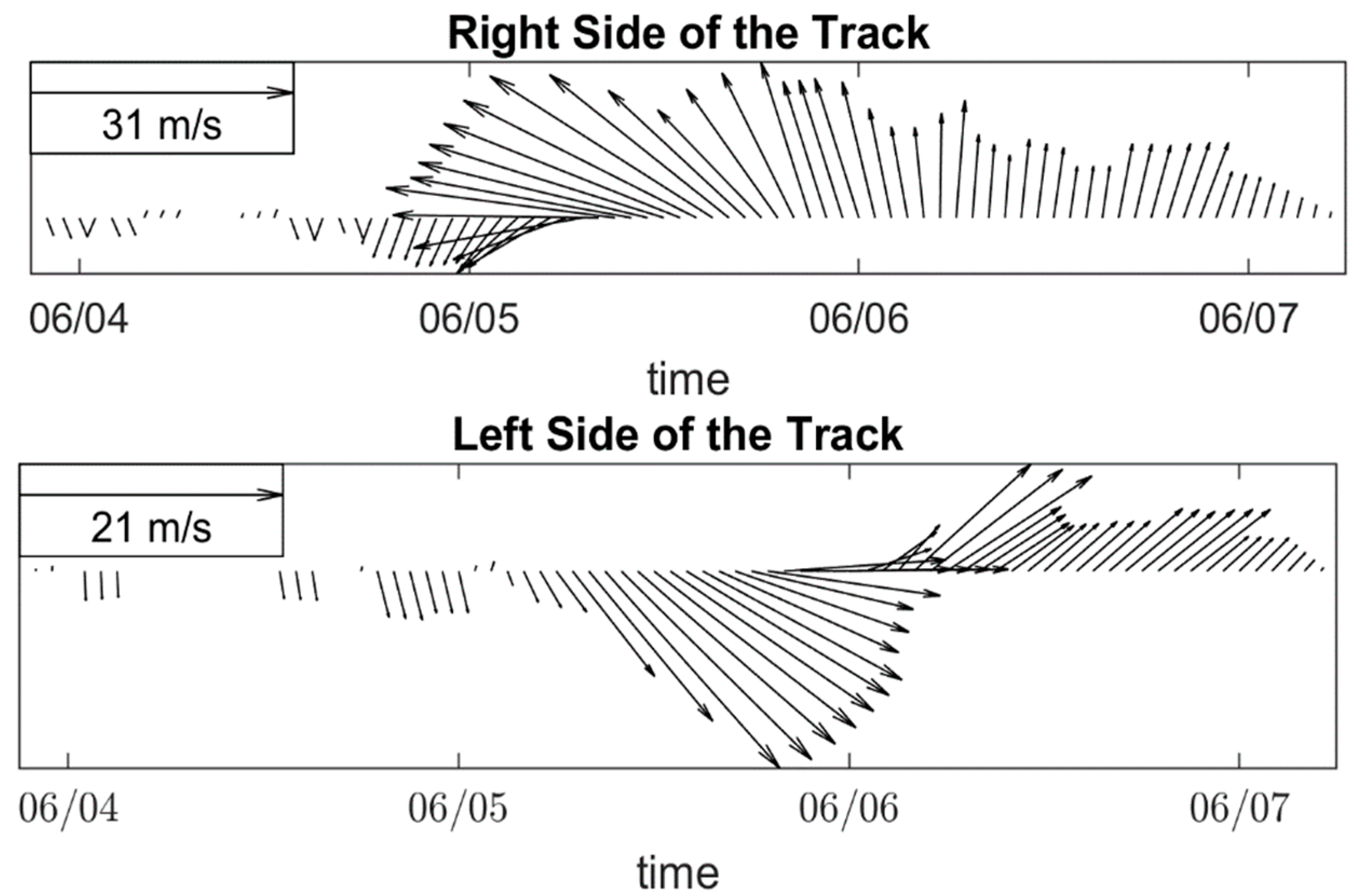
34]. On the left side of the track, time variations of wind-stress vectors are counterclockwise, that contradict the clockwise inertial currents and suppress them. The conditions for resonance are most favorable on the front right side of the cyclone, and thus the largest SST cooling is usually found in this region. For Cyclone Gonu, timeseries of wind vector variations at locations on the right and left sides of the track showed a similar pattern (
Figure 4). Wind vectors were plotted for points 3 and 4 in the Gulf of Oman (
Figure 1b) and were obtained from a Gonu wind field reconstructed based on the approach of Holland (1980) that was used by [
5] for a wave modeling study in the region.
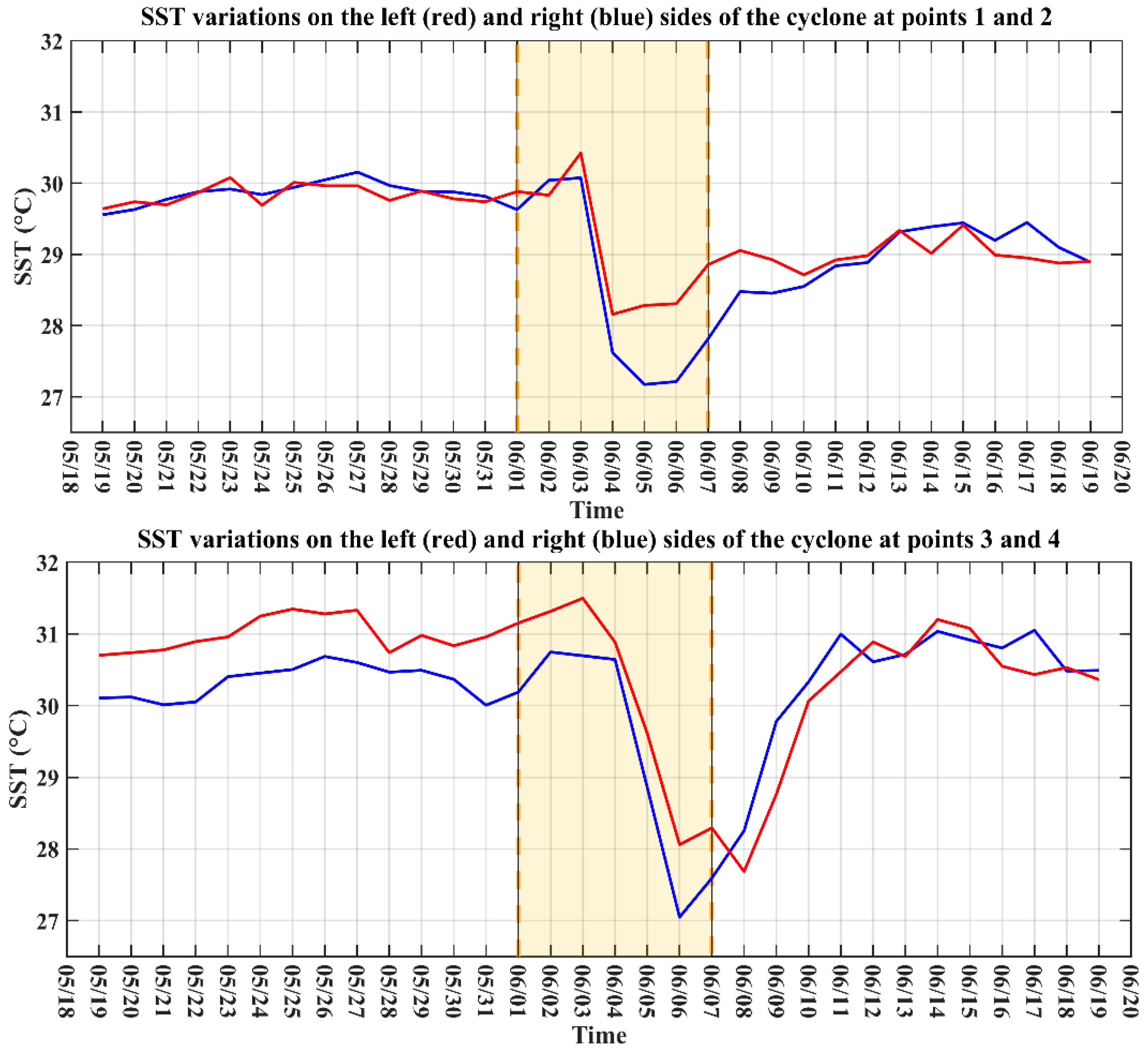
Hence, the maximum SST cooling is expected on the right side of the track, but it could also arise from the relative location of the cyclone’s track and land, or due to pre-existing cold- or warm-core eddies that can interact with cyclone-induced mixing [
24]. To examine Gonu’s induced SST cooling on the right side of the track versus the left side, 31-day SST timseries were compared at the right and left sides of the track (
Figure 5). Two pairs of locations (1 vs. 2 and 3 vs. 4) on either side of the track (see locations for points 1-4 in
Figure 1b) were compared. Timeseries include SST variations from 13 days before the formation of Gonu, 6 days of Gonu’s active period, and 12 days after landfall. Gonu passed over points 1 and 2 (located southeast offshore of Ras al Hadd) at 18:00 UTC on 5 June and passed over points 3 and 4 (located in the Gulf of Oman) at 00:00 UTC on 7 June. At both pairs of locations, the SST on the right side of the track during 1–7 June was lower than on the left side. The maximum differences corresponded to the time that the cyclone passed over the points. For points 1 and 2, this difference was 0.9 °C and for points 3 and 4 it was 1 °C. At these locations 3–5 days after the cyclone’s landfall, SST on the right and left sides approximately matched. However, SSTs at points 1 and 2 were still cooler than the pre-cyclone values, even 12 days (19 June) after the landfall. For the locations in the Gulf of Oman (3 and 4), return to pre-cyclone SST occurred about 5 days (12 June) after the landfall. The delay in SST rebound for points 1 and 2 could be due to stronger oceanic response within the mixed later and more intense upwelling due to the stronger cyclone winds at the time that the eye passed over these locations.
5. Calculating Gonu-Induced MLD
The methodology of
Section 3.1 based on Pan and Sun [
25] was used to estimate Gonu’s induced MLDs over the study region using SST data. According to Pan and Sun [
25], post-cyclone MLD can be calculated when the pre-cyclone temperature profile is known. However, direct measurements of pre-cyclone temperature profiles throughout the water column may be available for only a handful of locations through Argo data. As an alternative, monthly mean temperature profiles of water temperature, which are available through WOA, can be used as the pre-cyclone condition [
14,
25]. MLD was calculated within the affected area from 1 to 7 June. For each day, satellite SST data and WOA temperature profiles at different locations with different distances from the center of the cyclone were used in Equation (1) to calculate the corresponding MLD values.
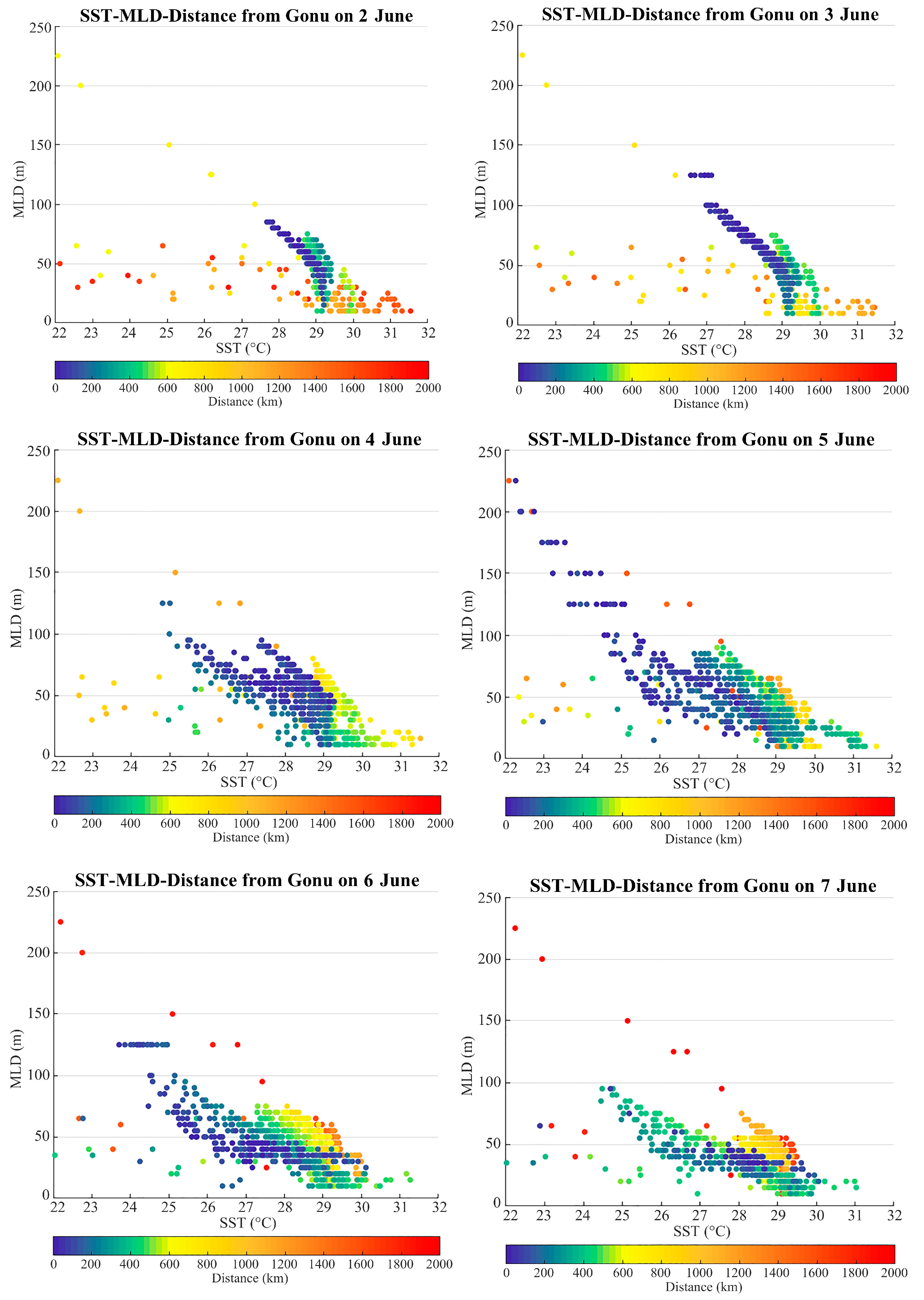
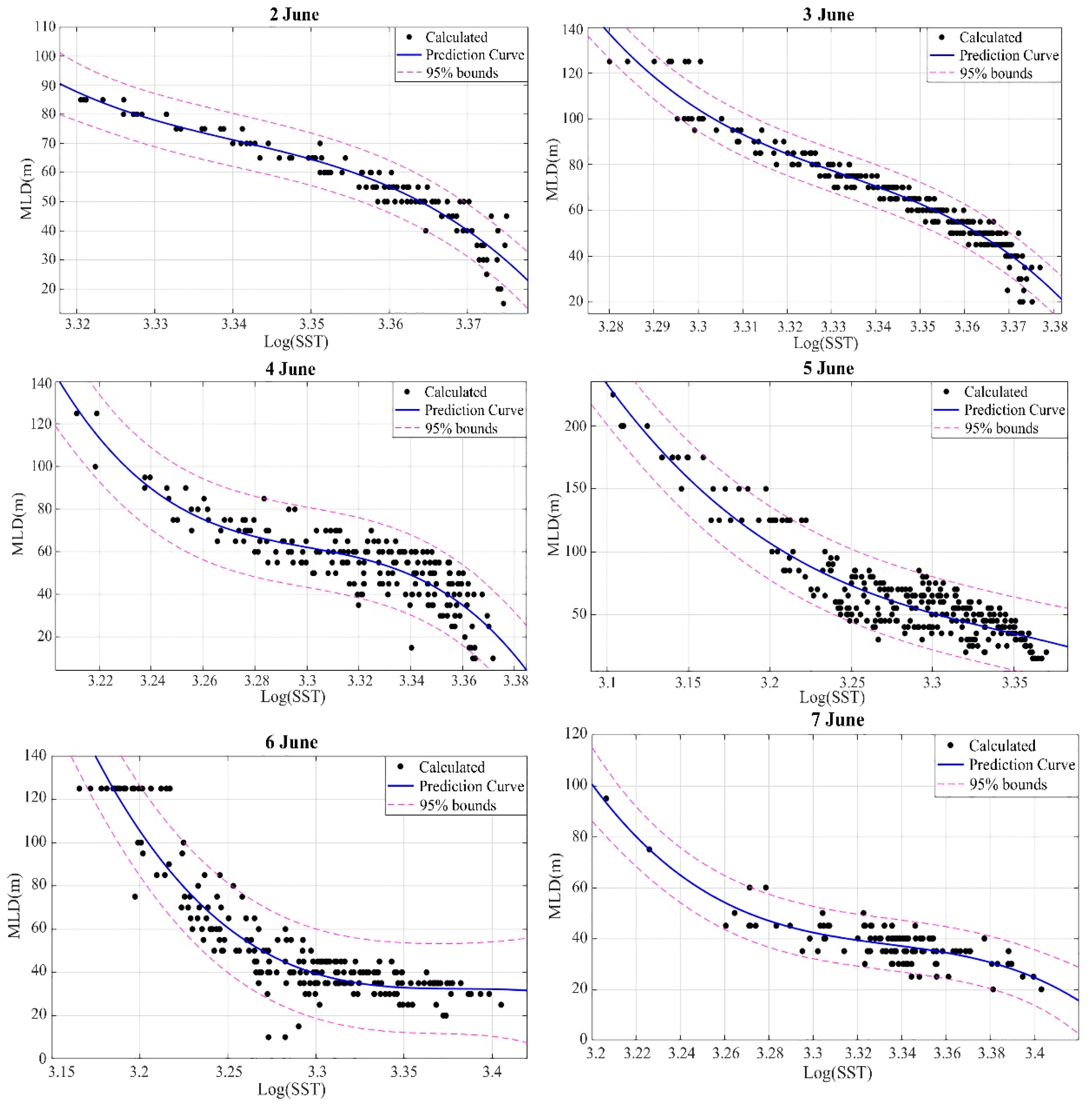
Figure 6 illustrates the scatter plots of MLD versus SST values on each date as a function of distances from the cyclone’s center (colors of the scatter points show different distances from the cyclone’s center). The distance from the track/center was considered as a contributing parameter in MLD calculations, since the mixing strength of the cyclone decreases with increasing the distance from the track/center. The results demonstrate that there could be a strong relationship between SST and MLD within a specific range of distances from the cyclone track and/or center on each date (herein called Distance of Influence (DOI)). The SST-MLD relationship generally became less predictable as this distance increased. DOI changes as cyclone intensity changes. A DOI of 200 km resulted in consistently high correlations for all dates (
Table 1). Considering the correlation only for locations for which DOI < 200 km, the log (SST)-MLD plots (
Figure 7) were resulted for different days. According to the results, a 3rd order polynomial curve was the best fit for the dataset. The only exception was for 1 June (not shown) for which a second-order curve fitted best. This could be because on 1 June the cyclone was still a tropical depression with no specific radius of maximum wind and inner structure, so the calculations were done within a smaller DOI with smaller number of points.
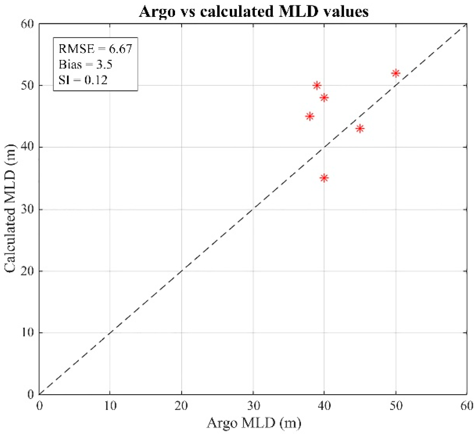
Evaluation of the calculated MLDs versus the limited numbers of Argo measurements that were available between 1–7 June (
Figure 8) showed an appropriate accuracy in calculating MLD, with an RMSE of 6.67 m that resulted in 15% of average error in calculating the MLD. This amount of error is acceptable considering the assumptions used to simplify the oceanic heat balance equation and derive Equation (1). It shows that this approach can be used for a quick estimation of the MLD during hurricanes/cyclones without a need for running the costly, time-consuming simulations using numerical models. MLDs were calculated using the relationships of
Table 1 for each day within a 200 km buffer around the cyclone’s track/center from 2 to 7 June (
Figure 9). The shape of a buffer zone and, consequently, the number of the calculation points for each day directly depends on the intensity of the cyclone and how close the track is to land. Therefore, the zones may be stretched (like 4 June) or almost round (like 2 June). According to these calculations, MLD started to deepen on 1 June (not shown) when Gonu started to form as a tropical depression. The deepening was intensified as the cyclone upgraded to higher Saffir-Simpson degrees on 2 June. MLD reached about 140 m on 4 June, when Gonu was at its most powerful. If the MLD deepening was mostly due to turbulent mixing induced by the cyclone, the deepening should correlate with the cyclone’s strength when other factors such as the forward speed of the cyclone remain the same. Nevertheless, the deepest MLD was calculated offshore of Ras al Hadd on 5 June when Gonu’s strength was declining compared to 4 June. Several reasons could contribute to this unexpected result, including the presence of pre-existing cold-core eddies in this area and/or extension of the coastal upwelling zone (prior or even during the cyclone) offshore of Ras al Hadd. The effect of pre-existing eddies will be discussed in the next section. The distribution of MLD around the cyclone center is asymmetric, which is compatible with the rightward bias discussed in
Section 4, especially for days corresponding to the maximum cyclone intensity, and following degrading phase (4, 5, and 6 June). On these days, the deepest MLD values, as well as the broadest deepened area (wherein the cyclone deepened MLD), were located on the right side of the cyclone’s track.
6. Effects of Pre-Existing Eddies on MLD Calculation
As seen in
Section 5, due to the lack of measured temperature profiles for the pre-cyclone conditions over the study area, the gridded monthly climatological profiles through WOA were used for determining the SST-MLD relationships and preparing maps of MLD. Using available Argo measurements as ground truth, we determined that an acceptable accuracy was achieved (
Figure 8). However, if the real pre-cyclone temperature profile is significantly different from climatological conditions, using the WOA profiles can cause substantial inconsistencies in calculating MLD [
25]. Deviations from climatological conditions can be caused by several factors, including changes in the heat/momentum balance of the region as a result of local storms or across-shelf transport by mesoscale eddies. These mesoscale eddies may include both cyclonic cold-core eddies (CCE) and anticyclonic warm-core eddies (WCE). The main feature associated with a CCE/WCE is upwelling/downwelling zones beneath the eddy core, resulting in rising/sinking of the thermocline [
25,
35]. This rising/sinking of the thermocline decreases/increases the pre-storm MLD and modulates the temperature profiles that directly affect the post-storm MLD calculation using Equation (1). By employing a numerical model of ocean turbulence, Pan and Sun [
25] showed that a 20 m rise in the thermocline as a result of a pre-existing CCE may cause a 30 m error in calculating MLD when the climatology profile is used as the pre-cyclone profile. Their estimation was done in the South China Sea during Typhoon Cimaron (2006) over an area with a 3 °C typhoon-induced cooling. Pre-existing oceanic eddies can also significantly change the cooling pattern around the cyclone center. Guan et al. [
24] reported that during Typhoon Tembin (2012) in the South China Sea, a pre-existing CCE on the left side of the typhoon’s track caused an abnormal leftward bias of surface temperature cooling with maximum cooling on the left side of the track 40–100% larger than the right side.
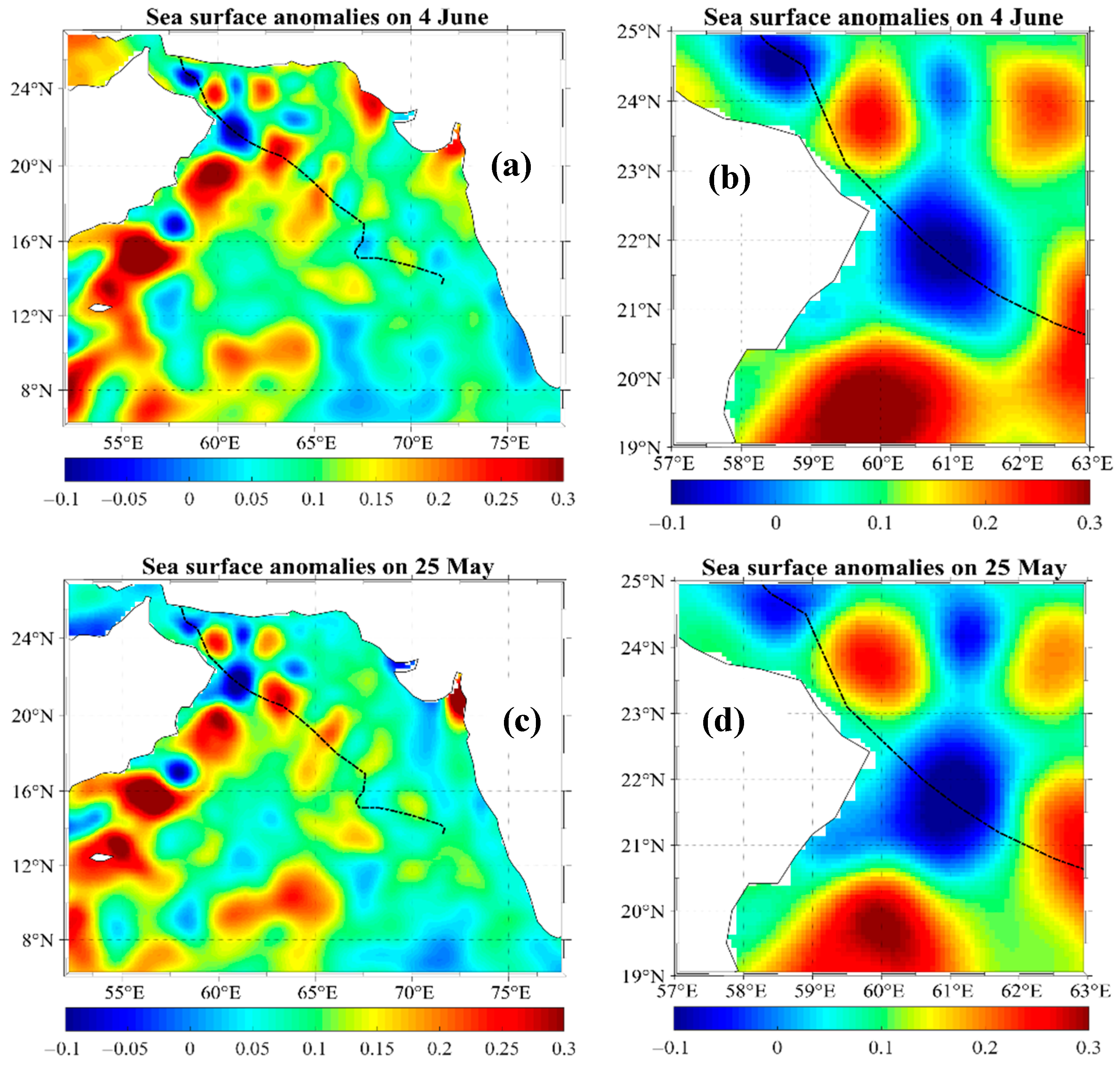
Mesoscale eddies are a prominent feature of circulation in the northern Arabian Sea, especially in the Ras al Hadd region along and off the coast of Oman [
36,
37]. This could affect the MLD calculations presented in
Section 5, especially on 4 and 5 June when Gonu’s track was close to Ras al Hadd. Maps of sea surface height anomaly (SSHA; data from the Copernicus program) for a week before the formation of Gonu (25 May) as well as the days after it (4 June) clearly showed that persistent CCEs and WCEs were present in the NAS (
Figure 10). As mentioned in
Section 5, the maximum calculated MLD using Equation (1) on 5 June was inconsistent with those calculated for 4 June. While the cyclone degraded on 5 June compared to 4 June, the maximum calculated MLD for 5 June (200 m) was substantially larger than that of 4 June (120 m). This unreasonable overestimation of MLD on 5 June can be explained based on the SSHA maps of
Figure 10. The figure shows a CCE extending from the eastern coast of Oman and Ras al Hadd almost to the offshore area with an associated sea surface height anomaly of −0.1 m or less. This pre-existing eddy coincided with the track of Gonu on 5 June when the eye was located offshore of Ras al Hadd. The CCE’s smaller SST (see
Figure 2e for SST map on 5 June) compared with the WOA climatological profiles was interpreted as excessive turbulent mixing in Equation (1) and irrational values for MLD resulted. This supports the idea that in the presence of pre-existing mesoscale eddies, Equation (1) should be used cautiously, as mentioned by [
25].
Figure 10 also shows several other CCE and WCE over the NAS and Gulf of Oman that were located on or in the vicinity of Gonu’s track. These eddies likely affected the accuracy of MLD calculations on 4, 6, and 7 June. However, the SST variations (
Figure 2) associated with these eddies were not as large as those due to the CCE located off Ras al Hadd.
7. Effect of Spatial Variability in Climatological Profiles
Examining spatial variations of WOA data used as the pre-cyclone profiles in the calculation of MLD can explain why the accuracy of correlations between MLD and SST on different days were different.
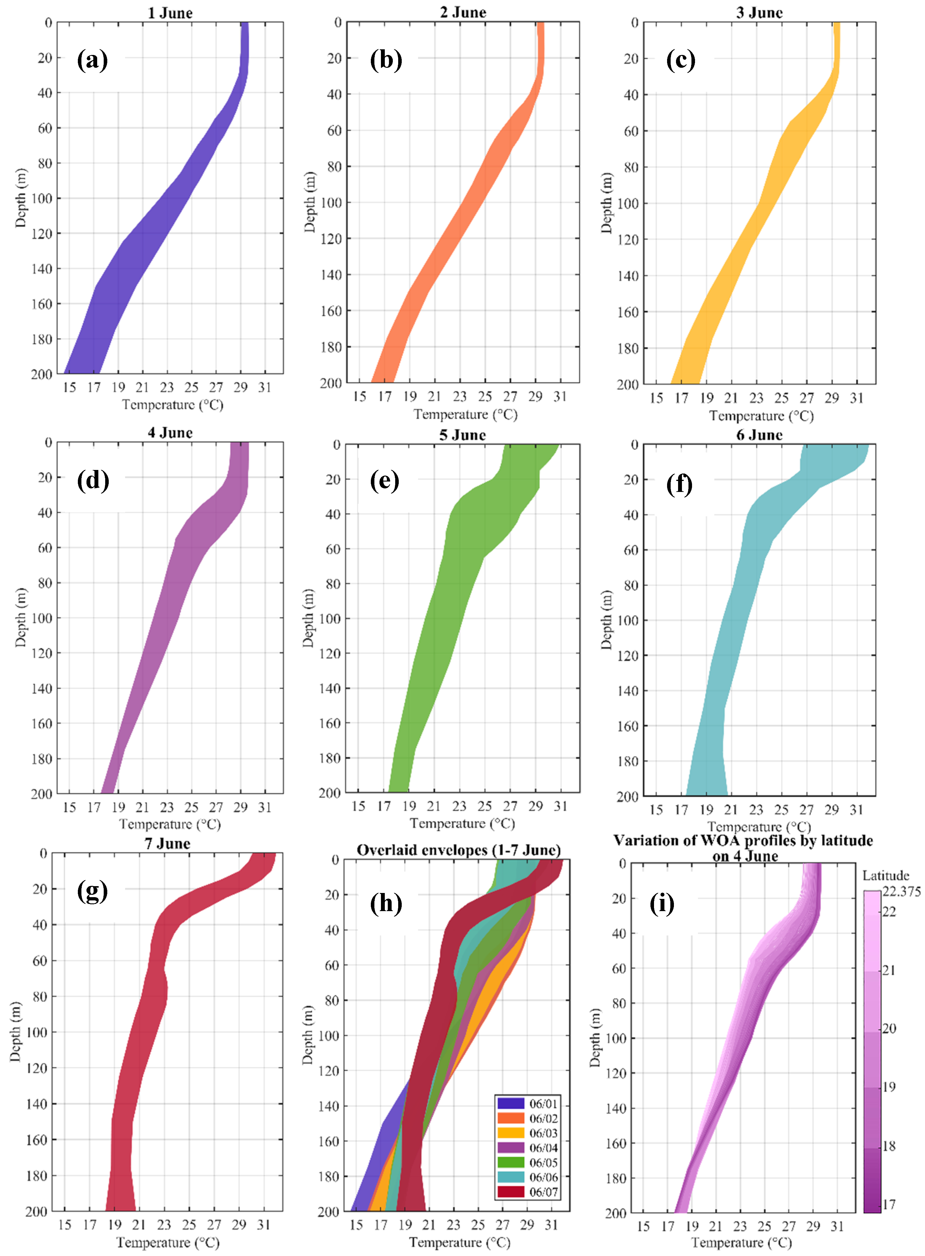
Figure 11 illustrates the envelope of WOA’s temperature climatological profiles of each day from 1–7 June within the DOI (zones shown in
Figure 9) for the upper 200 m of the water column. The envelopes include all the measured profiles for a specific day within that day’s DOI. Wider envelopes show that the shapes of the profiles were more spatially variable, and thus represent a more active area in terms of hydrodynamics and heat transfer processes. This directly affects the MLD calculations using Equation (1). For narrow envelopes, similar values of SST at two distinct locations within the DOI result in similar values of MLD, so less scattered points in log (SST)-MLD plots (
Figure 7) are observed. The high correlation (
) of the SST-MLD equation for 1, 2, and 3 June (
Table 1) is consistent with the narrow temperature profile envelope for the DOI corresponding to these days (
Figure 11a–c).
generally decreased when the cyclone reached higher latitudes on 4–7 June with a wider climatological profile envelope (especially on 5 and 6 June). Evidence of lower variability of hydrodynamics and heat transfer over the lower latitudes (corresponding to the location of the cyclone on 1–3 June) is the near absence of CCE/WCE at these latitudes for the period that Gonu translated the study area (
Figure 10). Conversely, for the higher latitudes, especially off the coast of Oman and in the Gulf of Oman, several persistent CCE and WCE were observed. Additional evidence of the high variability of oceanic heat transport along the coast of Oman and the associated offshore regions is the persistent seasonal upwelling that occurs during the summer monsoon [
29], which was active right before Gonu’s formation (see
Figure 2).
Variations of the WOA’s temperature profiles with latitude (
Figure 9i) within the DOI of 4 June show that as the cyclone moved toward higher latitudes, the profiles shift to lower temperatures. However, the shift was uneven over depth so that temperature decreased 1 °C in the upper 30 m while it decreased up to 4 °C at 50 m. Therefore, as the vertical mixing penetrated to lower depths, SST-MLD values became more scattered on 4 June (and similarly 5 and 6 June) because the integral part in Equation (1) should be calculated for a variety of temperature profiles within the DOI. The above discussion shows that substituting climatological profile data like those of WOA for the pre-cyclone profile in Equation (1) results in the best correlation of SST-MLD over the regions where spatial variability in hydrodynamics and heat transfer are minimal.
8. Effect of Using Climatological Profiles in MLD Calculation
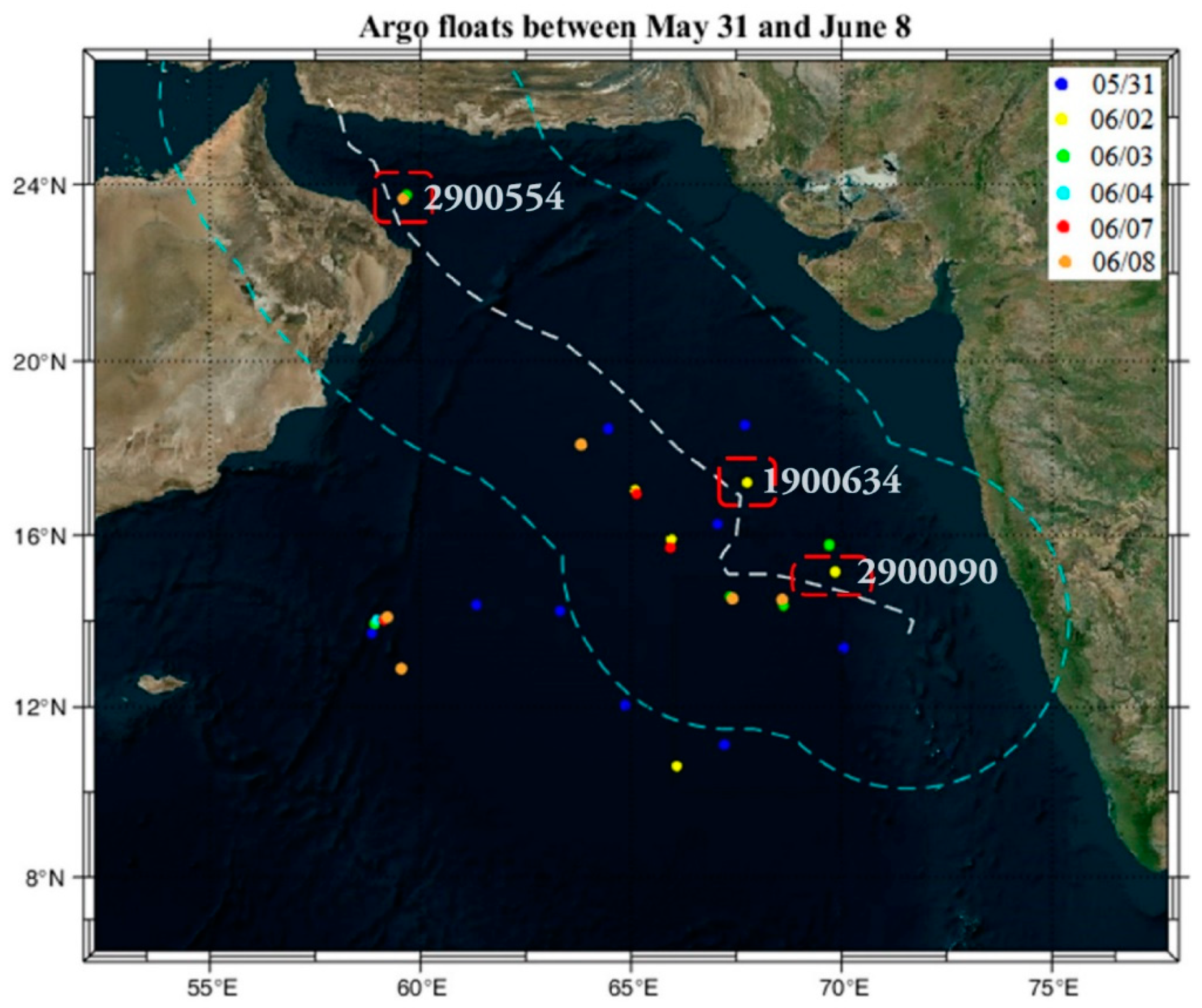
WOA represents long-term averages for temperature and salinity profiles which may differ from the real profiles at the time of MLD calculation. Therefore, it is important to evaluate the differences associated with using WOA profiles instead of measured temperature profile as the pre-cyclone condition. Both calculated MLD and temperature profiles were used for this evaluation.
Figure 12 shows the locations of Argo measurements which are utilized for this evaluations. Argo float 1900634 has measurements on 2 June. At this location, measured SST by Argo was 29.8 °C and the SST from the WOA profile was 30.2 °C. These SST values resulted in the calculated MLD of 64 m for Argo and 59 m for WOA as the pre-cyclone water temperature profile respectively. This is corresponding to a 7% difference when using WOA profile instead of the measured temperature profile.
Further analysis was performed to determine the differences in the temperature profiles presented by Argo and WOA data. The relative differences in percent were calculated across the water depth from 5 to 200 m as:
where in
T(
W) and
T(
A) refer to the temperature values of WOA and Argo profiles, respectively. The profiles and differences are shown in
Figure 13 for floats 2900090 (2 June in the Arabian Sea) and 2900554 (3 June in the Gulf of Oman) for the upper 200 m of the water column. The results show that for the location in the Arabian Sea, WOA’s temperature values across the upper water column are smaller than Argo profiles, with the maximum difference less than 4%. In the Gulf of Oman, WOA shows larger temperatures for the higher 40 m of the water column. The largest differences are about 10%. This shows that WOA profiles appropriately represent the temperature variations across the water depth which is consistent with other studies like that of Pan and Sun [
25].
9. Mixed Layer Deepening and Vertical Mixing
In previous sections, we showed through calculated MLD that during Cyclone Gonu, the areas around the cyclone’s center within a specific radius (DOI) were affected by cyclone-induced mixing. The temporal variations of MLD at each location within a DOI account for the overall intensity of the mixing. However, these variations reveal nothing about the rate of exchange of turbulent energy across the water column. Nevertheless, it is imperative to examine the consistency of the calculated MLD based on the MLD-SST approach and the estimated rates of the turbulent energy transfer across the water column. The transfer rate is usually represented by diapycnal diffusivity [
24] and can be calculated using the measured vertical profiles of temperature and salinity using the method suggested by Kunze et al. [
38]:
where
,
, and
is the ratio of shear and strain for which the value of 7 was suggested by Kunze et al. [
38].
is the strain variance of the internal waves as obtained from Argo data, and
is a standard strain variance based on the Garrett-Munk spectrum of internal waves as specified by Garrett and Munk [
39]. For the Argo data, strain is calculated using the buoyancy frequency
as:
The above formulations were derived based on the internal wave-wave integration theory originally validated by Gregg [
40] against real oceanic observations and was formulated with both shear and strain variance of internal waves. For the present study, the vertical profiles from Argo floats were used to calculate diapycnal diffusivity using Equation (3). Comparing the estimated
K values at a specific location and different times (before, during, and after the cyclone affected that location) could provide a great opportunity to quantify the time evolution of vertical mixing induced by Gonu. Unfortunately, Argo measurements in the study area during Gonu were few (
Figure 1 and
Table A1), so accomplishing this was not possible due to scattering and scarcity of data. For comparison of the diapycnal diffusivity in this paper, the most appropriate data were found through Argo float 2900556, located within the longitude range of 63.8°–63.9° E and latitude range of 18.0°–18.1° N (marked with a red circle in
Figure 1). Measured temperature and salinity for this Argo float are available for 3, 8, and 13 June. Thus, the measurements can be used to calculate the difference between the vertical turbulence rates at different times for this location. The distance between the Argo float and Gonu’s center on 3 June was 250 km. Gonu made landfall before 8 June; therefore, measurements on 8 and 13 June show the post-storm conditions.
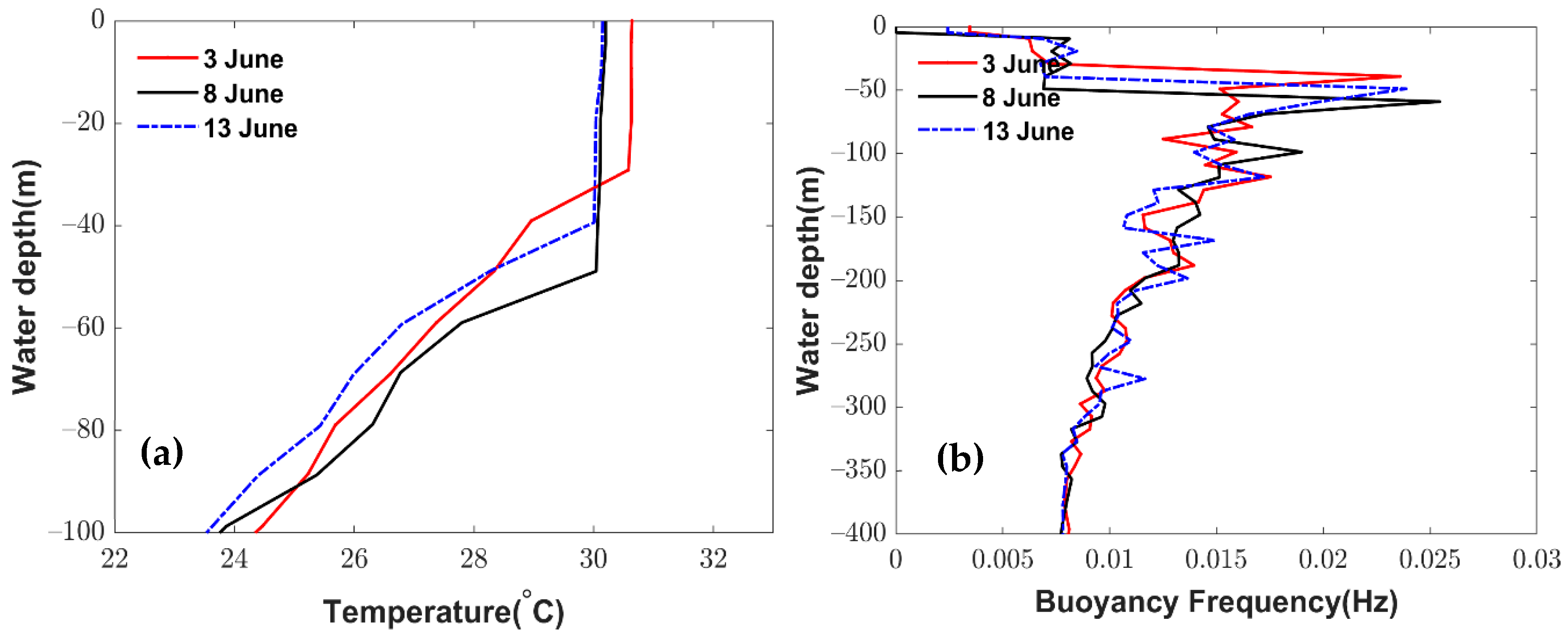
Figure 14 shows the measured temperature profiles on each of these three days for the upper 100 m of the water column. The MLD for 3, 8, and 13 June were 20, 55, and 45 m, respectively (
Figure 14a). The calculated buoyancy frequency (
Figure 14b) for the upper 400 m of the water column was consistent with the temperature profiles showing the formation of the thermocline at 20–50 m. The measured mixing depth of 30 m on 3 June is consistent with the calculated 25 m MLD (
Figure 9) for 3 June at the location of the Argo float. Although on 8 June no MLD map was calculated due to Gonu’s landfall on 7 June, the MLD map for 4 June (when the cyclone significantly strengthened) showed a 65 m calculated MLD at the location of this Argo float which is comparable with the measured MLD of 55 m on 8 June. The decrease in measured MLD on 13 June was expected because it was measured six days after Gonu’s landfall.
The temperature and salinity measured by Argo float at this location were used to calculate the diapycnal diffusivity for 3, 8, and 13 June. Following [
24,
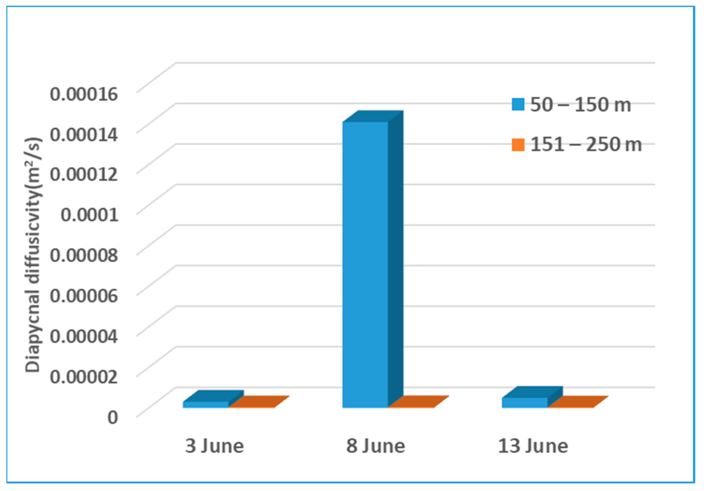
38], the calculation was done for the water column beneath the surface mixed layer (at approximately 50 m depth). Diffusivity was calculated for two 100 m portions of water column: 50–150 m and 151–250 m (
Figure 15). In the lower portion of the water column, diffusivity was almost constant on 3, 8, and 13 June, while in the upper portion, diffusivity on 8 June (1.4
10
−4 m
2 s
−1) increased 45-fold compared to 3 June (3.07
10
−6 m
2 s
−1). This significant increase of the diapycnal diffusivity for the upper water column was consistent with the large observed and calculated MLD at the location. As a result of this enhanced mixing across the water column, the warmer surface water went descended and the cooler subsurface water came up to the surface. Thus, beneath 35 m, the 3 June profile exhibited colder temperatures than those on 8 June.
10. Summary and Conclusions
Sea surface temperature (SST) and mixed layer depth (MLD) response to the historic category 5-equivalent Cyclone Gonu in the northern Arabian Sea (NAS) and Gulf of Oman were studied and delineated using satellite data and climatological temperate profiles. The maximum SST cooling produced by Gonu during 1–7 June 2007, when the cyclone was active over the study region, was 1.7–6.5 °C, generally consistent with the impact of a slow- to medium-moving cyclone as classified by Bender et al. [
1]. The maximum cooling of 6.5 °C off Ras al Hadd was consistent with the maximum intensity of a category 5 hurricane. SST maps and time series on two sides of the cyclone’s track showed asymmetrical patterns, with greater cooling on the right side due to the rightward bias effect.
To study the mixed layer deepening caused by Gonu, a fast and convenient method of estimating MLD during a cyclone/hurricane/typhoon was implemented and tested for the NAS and Gulf of Oman. The approach relies on SST data measured by cloud-penetrating microwave satellites and the pre-cyclone water temperature profile, with the main assumption that turbulent mixing resulting from the cyclone is the major force deepening the mixed layer. Although this hypothesis was successfully examined by Pan and Sun [
25] for the South China Sea, few discussions or results were presented about the details of the method’s implementation and the circumstances under which the method works or fails. The present study presents details of these calculations including the statistical variability of the correlation between SST and MLD, spatial variability of the relationships, and oceanographic conditions that cause uncertainties in calculating MLD. The results showed that the correlation weakened with increasing the distance from the track/center of the cyclone, and a distance of ≤200 km from the track/center resulted in the best correlation. Evaluation of calculated versus Argo-measured MLDs during Gonu’s passage showed that the accuracy of this method of MLD calculation was 15%, an acceptable accuracy for a fast prediction tool.
Pre-cyclone mesoscale eddies onshore and offshore of Ras al Hadd and inside the Gulf of Oman may have contributed inconsistency and uncertainty to the MLD calculations. These eddies and other active transport phenomena can cause errors in MLD calculations by deviating the pre-cyclone condition from the climatological profiles. Climatological profiles were used as the pre-cyclone profiles due to the lack of measured temperature profiles before the cyclone. The calculated MLDs over the study area were consistent with the time variations of the diapycnal mixing at a location in the NAS for which Argo data were available on three different days before and after the cyclone. The approach for estimating MLD in this paper provides a quick, inexpensive method for estimating cyclone-induced MLD with acceptable accuracy. This method can be used by fishery departments, environmental institutes, and bio-geochemical scientists before relying on costly 3D circulation models. MLD is important in the context of water column re-oxygenation during a cyclone. The NAS has one of the most intense oxygen minimum zones in the world. Studies showed continuous declines in the oxygen concentration in oceanic waters in this region during recent decades, mostly attributable to the fast local increase in SST [
41]. Mixing caused by a cyclone can re-oxygenate the water column down to the mixing depth for several days to weeks after the cyclone’s passage [
42]. Therefore, estimating the MLD and its spatial distribution during a cyclone can provide a great metric for predicting the zones of re-oxygenation, which likely will be zones of high primary production within weeks to months of the cyclone’s passage.
The present study is one of the first studies to address upper ocean temperature response to a tropical cyclone in the NAS and Gulf of Oman. More studies are needed to address additional aspects of the region’s response, with further details. Studying mesoscale and sub-mesoscale mechanisms associated with the asymmetric cooling around a cyclone’s track and the role of these mechanisms on enhancing biogeochemical processes (as studied by McGee and He [
11]) over the study region will help shed more light on these responses. Use of numerical models and field data can address these mechanisms.
It should also be noted that the presented approach for estimation of the MLD using the mixed layer heat budget conservation is approximate and could be associated with some uncertainties. Although effect of the turbulent mixing on the mixed layer heat budget is dominant during tropical cyclones, for the slower-moving storms the effect of air-sea heat exchange and horizontal advection can increase. Since Gonu’s forward speed was slow to medium during the major times that it was translating the study region (see
Figure 3a), the estimation error is not substantial. However, for fast-moving storms more inaccuracies can be expected. The exact evaluation of this error should be examined through coupled ocean-atmospheric models which was not in the scope of this study.


