
3D Simulation with Flow-Induced Rotation for Non-Deformable Tidal Turbines

Morphodynamique Continentale et Côtière (UMR CNRS 6143), Université de Caen (Campus 1), 14000 Caen CEDEX, France
*
Author to whom correspondence should be addressed.
J. Mar. Sci. Eng. 2021, 9(3), 250; https://doi.org/10.3390/jmse9030250
Submission received: 29 January 2021
/
Revised: 19 February 2021
/
Accepted: 21 February 2021
/
Published: 26 February 2021
(This article belongs to the Section Ocean Engineering)
Abstract
:The overall potential for recoverable tidal energy depends partly on the tidal turbine technologies used. One of problematic points is the minimum flow velocity required to set the rotor into motion. The novelty of the paper is the setup of an innovative method to model the fluid–structure interactions on tidal turbines. The first part of this work aimed at validating the numerical model for classical cases of rotation (forced rotation), in particular, with the help of a mesh convergence study. Once the model was independent from the mesh, the numerical results were tested against experimental data for both vertical and horizontal tidal turbines. The results show that a good correspondence for power and drag coefficients was observed. In the wake, the vortexes were well captured. Then, the fluid drive code was implemented. The results correspond to the expected physical behavior. Both turbines rotated in the correct direction with a coherent acceleration. This study shows the fundamental operating differences between a horizontal and a vertical axis tidal turbine. The lack of experiments with the free rotation speed of the tidal turbines is a limitation, and a digital brake could be implemented to overcome this difficulty.
1. Introduction
Pushed by the energetic transition, a lot of countries are developing their sectors of renewable energies. Even though they represent 3/8 of the global wind energy potential [1], marine renewable energies have a number of advantages: The density of the recovered energy is higher with bigger wind turbines and less turbulent wind or tidal turbines in sea water. Fishermen are the first opponents to the implantation projects, yet the installation of wind or tidal turbine farms seems to favor the development of marine ecosystems owing to the reef and reserve effects [2]. Marine renewable energies have a huge potential with several thousands of TWh/month for offshore wind turbines alone [3]. Today, the tidal energy potential is less than that for wind or wave energies. Potentials are calculated depending on existing technologies, and as tidal turbines are more recent than wind turbines, their potential is less. Both technologies use a rotor that needs a certain amount of energy density to start. For that reason, new foil designs are proposed to allow turbines to start with lower speed flows [4]. Some other options include telescopic blades in order to control the momentum and the load as presented in Jamieson’s patent US6972498B2: “Variable diameter wind turbine rotor blades”. In such cases, the turbine starting point (the minimum flow velocity at which the turbine starts to turn) is critical for understanding the real contribution of such systems. Moreover, tidal turbines are often placed in bidirectional alternative flows, which subject them to numerous restarts.
This paper aims at introducing a method to simulate the flow induced by fluid–structure interactions applied on tidal turbines. This method allows one to study, at the same time, the turbine starting point, the acceleration phase and the turbine performance with a numerical approach.
Since its emergence in the 18th century, there have been two approaches in fluid mechanics: Eulerian [5] and Lagrangian modeling. For a free stream, Lagrangian models are more effective in terms of calculation time. However, when it comes to fluid–structure interactions, which are essential for studying energy recovery systems such as tidal turbines, particles badly interact with walls [6,7]. Therefore, Euler equations have spread faster in industry and the research community. They have been widely used to predict wind turbines’ [8,9] and tidal turbines’ [10] performance. With the development of computer science and the increase in computing capacity, numerical modeling has also progressed from one-dimensional to three-dimensional (3D) cases [11], passing through two-dimensional (2D) cases [12]. This last type is a good compromise between computation time and accuracy. Even if 3D models are more suitable for predicting turbine energy recovery than 2D, their computational costs are higher when solving the Navier–Stokes equations (around 30 times higher than 2D).
Simpler models have been developed to reduce these costs, mainly used first for wind turbines. The actuator disk [13], which does not take the blade design into account, can only be used to pre-evaluate the turbine production owing to its high rotor size, but its accuracy remains low. The blade element momentum method (BEMM) subdivides the blade into 2D foils with different lift and drag and deduces the total performance of the turbine from it. The BEMM is initially used to predict and improve wind turbine designs but can also be used for tidal turbines [14]. The method is limited by its poor management of 3D effects. Blade tip vortices are ignored, and it is not possible to account for large variations in blade thickness. The model has to be applicable to the study of high roughness on the blades (in particular, to be able to take into account biofouling). The lifting line theory method (LLTM) uses Kutta and Joukowski’s conditions on finite sections to compute the circulation around the blade and deduces its performance [15]. Vortex filaments are used to model the wake. This method requires strong conditions such as the flow being attached to the blade that are not respected by fouled blades. Coupled methods involving these prediction methods and Navier–Stokes codes have also emerged for predicting tidal turbine performance at a large scale [16], but they are subject to the same conditions.
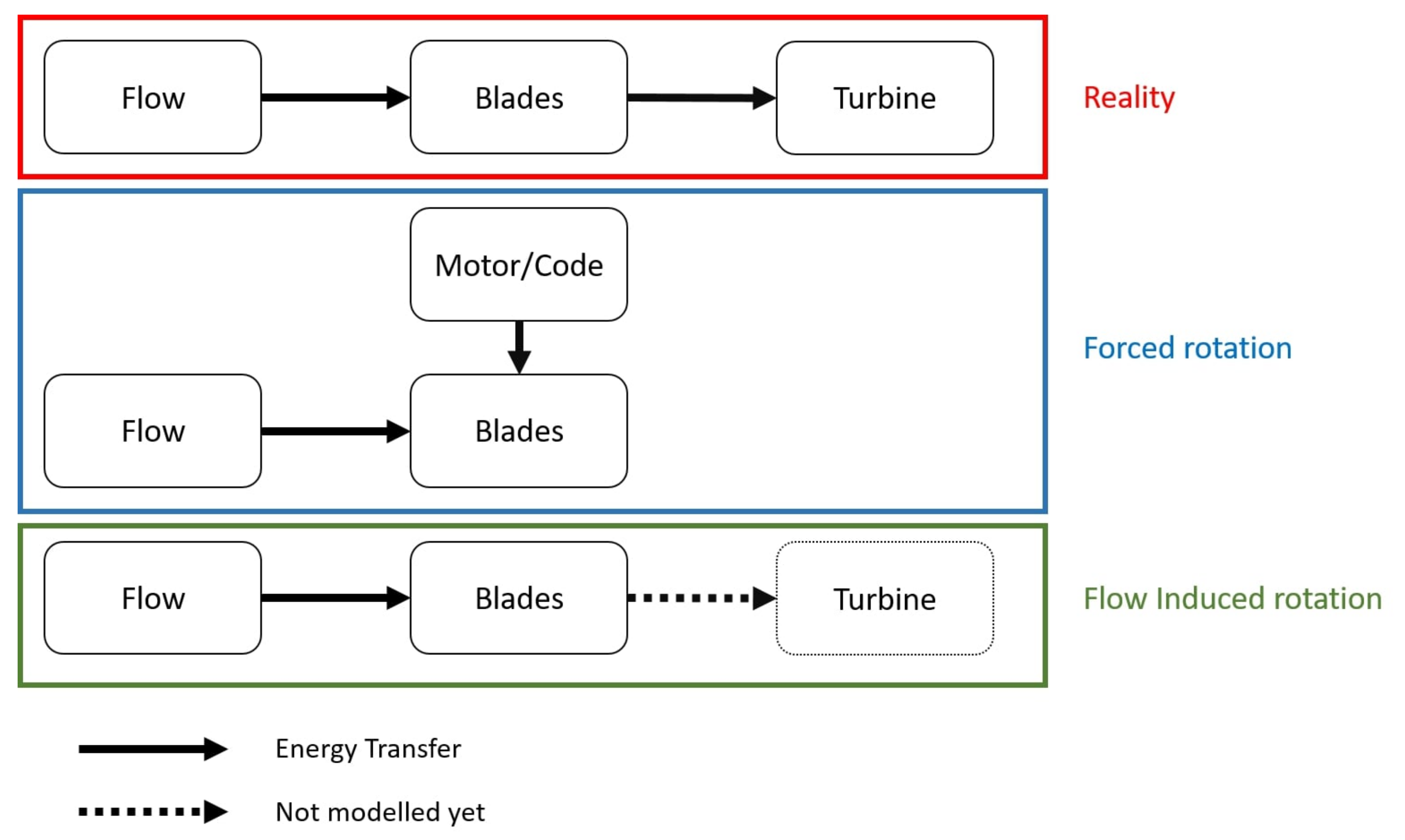
Despite the computation costs, a full 3D Eulerian Navier–Stokes simulation is the most accurate way to model the tidal turbine motion. This kind of approach has already been carried out in the past (e.g., [17]). Nevertheless, it is widespread to use a forced rotation to set the blades in motion, whether experimentally or numerically. This motion is effective for representing performance at certain operating points but does not respect the energy recovery chain: energy is provided by the rotor engine or by the code according to the type of experiment. This does not allow studying the starting points of turbines or their acceleration. Flow-induced rotation is more respectful of the energy recovery chain: both kinetic and converted energies come from the stream. We propose simulating the flow-induced rotation of the tidal converter. From what we know, this aspect has still not been addressed. Flow-induced solvers have already been used to compute a heaving buoy [18] or a floating ship [19] but not in an energy recovery system.
In this work, the turbine was considered as a non-deformable solid. This means that the blades do not bend under the forces applied by the fluid. The distance between each point of the solid is constant. In fact, when they rotate, the blades of tidal turbines are under high stresses, and therefore, they are deformed [20]. However, this type of interaction makes the problem much more complex. Solving the deformations requires a high computing time because the calculation code must be able to solve the fluid and solid deformation equations.
After a short introduction, Section 2 presents the methodology pursued. The experimental setups are first described, and then, the governing equations are detailed.The difference between flow-induced rotation and forced rotation is explained. The boundary and initial conditions are given, and 3D geometries and meshes are presented. Section 3 is dedicated to the mesh convergence, the model validation with experimental data, and the flow-induced simulation. Conclusions are drawn in Section 4.
2. Methodology
2.1. Experimental Setup
2.1.1. Horizontal Axis Tidal Turbine Experimental Setup
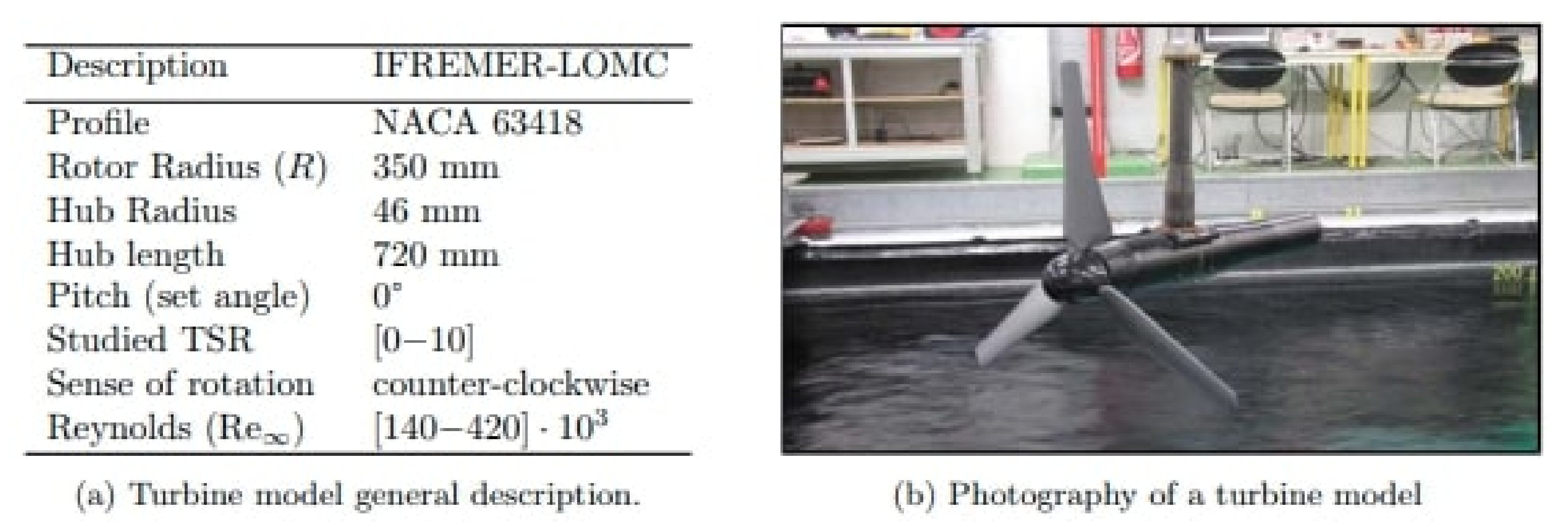
The numerical simulations were built to reproduce the laboratory experiment of [21], which we briefly describe hereafter. IFREMER (the French Research and Sea Exploitation Institute) facilities were used for the lab experiment. The flume tank size was m and could generate a stream-wise flow velocity of 0.1 to 2.2 . Two turbulence intensities were tested ( and ). The turbine was set in motion by a motor that forced the rotation speed and controlled the tip speed ratio (TSR). The TSR is a nondimensional number used for turbine studies, defined as the ratio between the rotor tip velocity and the upstream flow velocity:
where is the angular velocity, R is the radius of the tidal turbine and is the inlet flow velocity.
The IFREMER-LOMC (LOMC is the Waves and Complex Environment Laboratory in Le Havre) turbine characteristics are given in Figure 1. More details about the twisted blades are given in [21].
Power and drag coefficients were measured using a torque sensor rather than a load cell. The wake was monitored with an LDV (laser Doppler velocimeter) system. The experimental trials included the hub and mast. The torque measurement included forces on these parts. The load and wake characteristics are shown and compared in Section 3.
2.1.2. Vertical Axis Tidal Turbine Experimental Setup
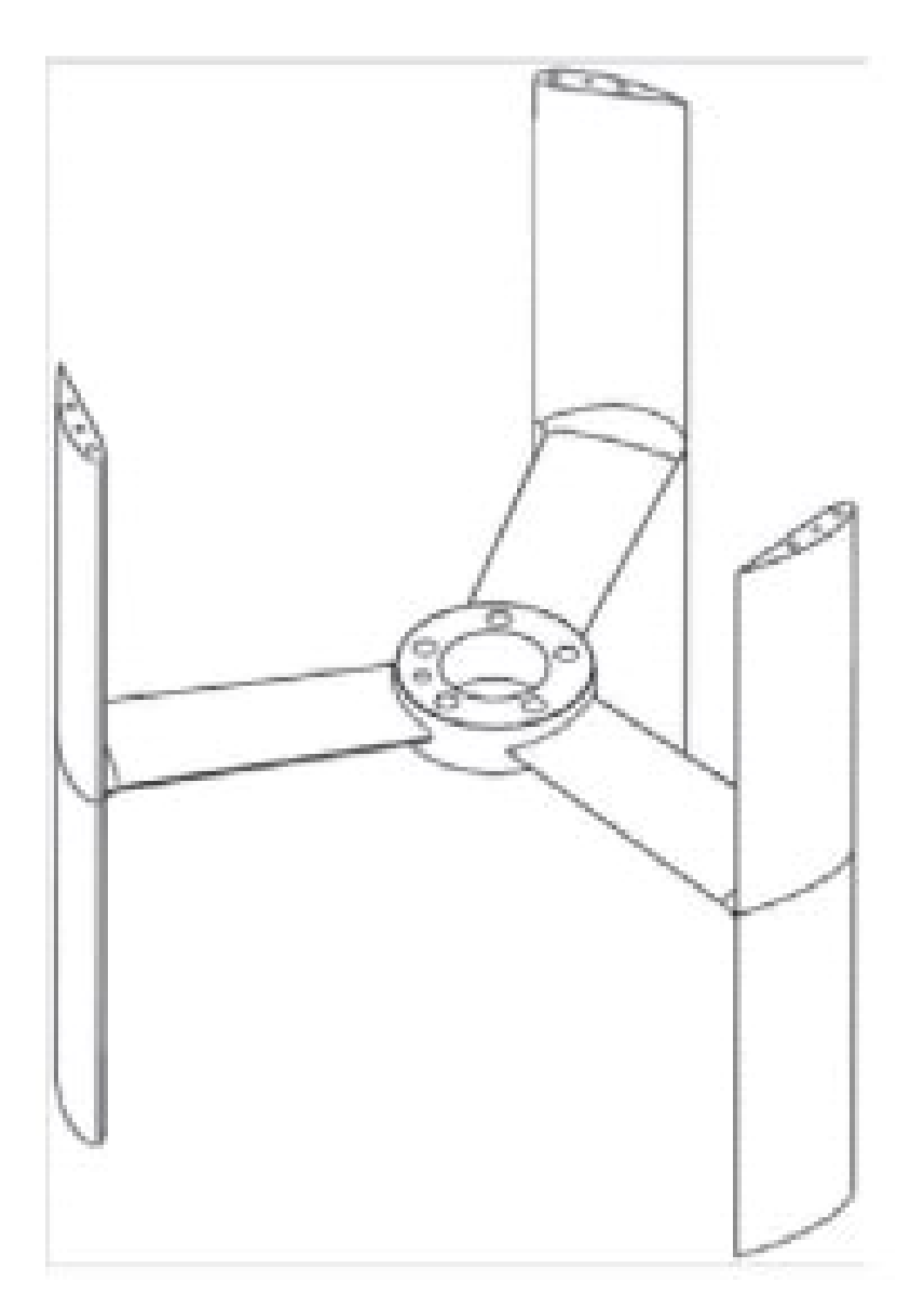
Numerical simulations were also performed for the Darrieus vertical turbine presented hereafter. This turbine following the A-10 geometry was built during the HARVEST program [22]. The blades are straight and built from a 0.032 chord NACA0018 profile foil. The profile is projected on the turbine rotation circle.
The model was a 1:5 scale of the original turbine [23]. The rotor was 0.175 in height, and its diameter was 0.175 (Figure 2). The inlet flow was water moving at . Laboratory tests were performed in the current flume of LEGI (Grenoble-Alpes University and CNRS), and a motor was used to force the turbine rotation to reach TSRs of , and . The trials aimed at studying the impact of various fairings on the tidal turbine performance. A free turbine experiment was carried out as a reference case. The complete structure also included a mast and three diametrical blades. We used the laboratory data in Section 3 for the comparison with the model results.
2.2. Governing Equations
This study used the 3D Eulerian Navier–Stokes equations for solving the motion of an incompressible fluid (for ):
where is the fluid velocity in the i-direction, t is time, is the fluid density (), p is the pressure, represents the volumetric forces and is the kinematic viscosity.
The authors of [12] show that turbulence can be solved with accuracy using k--SST (shear stress transport) or LES (large eddy simulation). In this study, the Smagorinsky LES model [24]) was chosen because of its capacity to predict the formation and the transportation of the vortexes.
LES is based on a flow separation into two parts by applying a spatial filter (see Equation (4)) such that:
where represents the turbulent structures whose length scales are larger than the filter width. These structures are explicitly solved. By contrast, is for structures with length scales smaller than the filter width, and the effects of these structures are parameterized.
The Smagorinsky scheme uses a discrete spatial filter. The Navier–Stokes equations can then be written as [25]:
where , and are the filtered pressure, deformation tensor and volumetric forces, respectively. is the turbulent eddy viscosity. is the width of the filter.
In OpenFoam, is given by
where k is the turbulent kinetic energy computed according to:
with being the tensor of deformations.
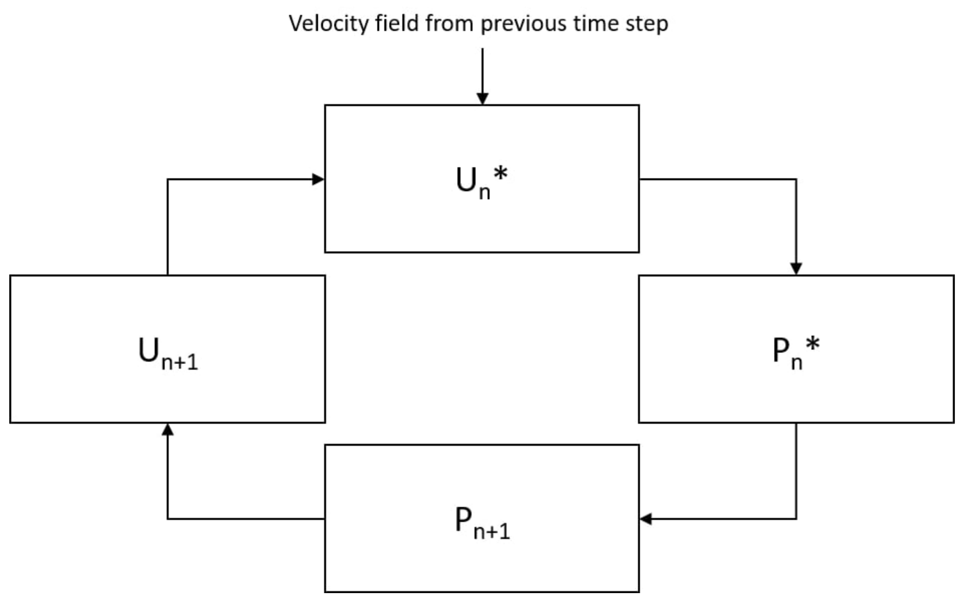
PimpleFoam was used as a fluid solver, and it is described in the OpenFoam documentation [26] as a “Transient solver for incompressible, turbulent flow of Newtonian fluids on a moving mesh”. It is based on an algorithm coupling velocity to the pressure equations. Equation (8) was used to construct a first estimate of the velocity . The pressure, P, was deduced from Equation (9) using .The velocity matrix could then be corrected. This operation was repeated until the solution reached the convergence criteria, which were set to for the error, before moving to the next time step (Figure 3).
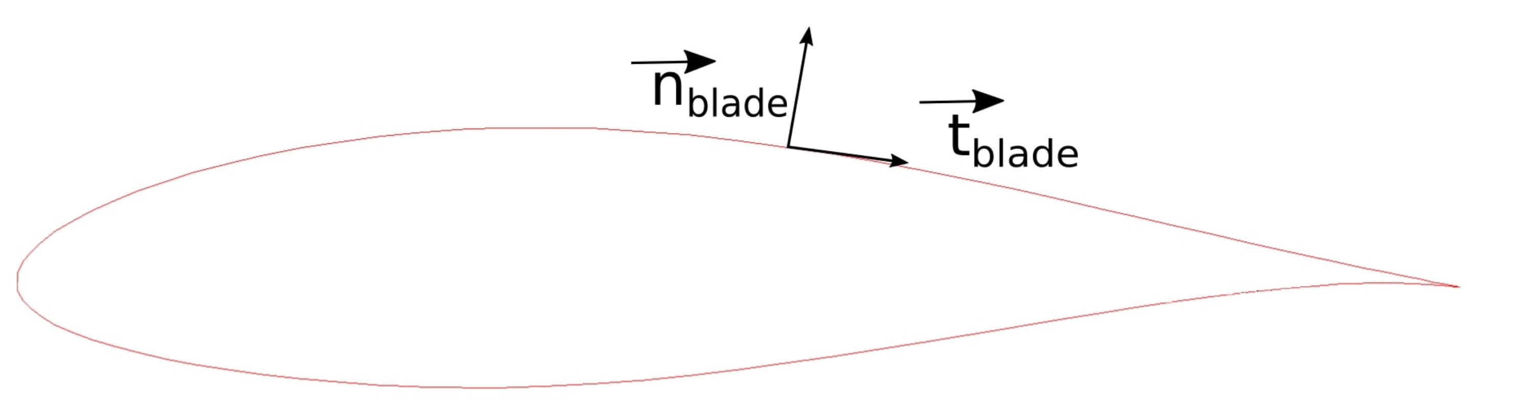
The motion of the structure was computed using the module named sixDoFRigidBodyMotion, which was added to PimpleFoam to model the fluid–structure interaction. This module computes the forces acting on the blades and converts them into point displacement for the close-rotor mesh. Without this module, these point displacements are fixed with a constant value that constrains the rotation of the rotor at a certain speed. In our “forced rotation” cases, the sixDoFRigidBodyMotion module was disabled and the rotation speed was set to obtain a certain tip speed ratio. The forces on the blade could be retrieved (Figure 4). When the rotation was induced by the flow, the forces and momentum were calculated from the flow characteristics using Equations (10) and (11). They were then converted into acceleration or moments of inertia depending on the system constraints using Equation (12). When the system was stabilized at the final free speed, all the energy brought by the fluid was converted into rotation speed. The forces acting on the blades were, therefore, equal to zero.
where is the total force applied on the surface, and is the moment in the i-direction. and are surface normal and tangential vectors in the blade datum, respectively. and are the related norms. is the lever arm. The summation surface is the blade’s surfaces.
In the flow-induced cases, the rotor angular acceleration () was calculated using the following equation:
where is the moment of inertia. Note that in the case of a forced rotation.
In OpenFoam 6.x, solid and fluid equations are strongly coupled together within PimpleFoam in order to represent physical motions with accuracy. After the initialization phase of the flow, the forces and displacements were computed for each PimpleFoam iteration. When all the variables reached their convergence criteria, the model started a new time step. A more accurate description of the solver is available in [9]. The difference between forced and flow-induced approaches is shown in Figure 5.
Boundary and Initial Conditions
The numerical configuration was built to reproduce the laboratory experiments described in Section 2.1. The boundary conditions were:
Boundary conditions:
Meanwhile, the initial conditions were set to:
Initial conditions:
where is the computational domain, is the inlet, is the outlet and are the four other surfaces (bottom, up, front and back). is the normal vector of the surface on which it is applied.
Equation (13) describes the inlet velocity set to a constant value () that follows the x-direction. A pressure outlet value is given by Equation (14). A slip velocity condition was applied on the bottom, up, front and back surfaces (Equation (15)). Equation (16) was applied on the rotor surface. This equation is only valid in the rotor datum. The flow speed near the blades is equal to the rotor local rotation speed in the experiment datum.
Initial conditions were applied on the entire domain (Equations (17) and (18)). As the flow is supposed to tend to , the condition on the velocity could be set to this value. However, to improve the numerical convergence of the code, we preferred to let the flow develop itself by setting a zero velocity at . As PimpleFoam is a velocity–pressure solver, the pressure was solved with the velocity propagation.
2.3. 3D Geometries and Mesh
All the 3D blade geometries of this work were generated using the open source software QBlade [27]. The hub geometry was completed with Blender (open CAD software) to model the entire rotor and hub.
All the meshes were made using the meshing tool SnappyHexMesh of OpenFoam. They were unstructured except on walls where structured layers were added to control the boundary layer. A numerical flume was built to avoid side effects and to capture the turbulent wake. The AMI (arbitrary mesh interface) method used in [12] was activated to avoid mesh deformation during the rotor rotation.
2.3.1. Horizontal Axis Turbine
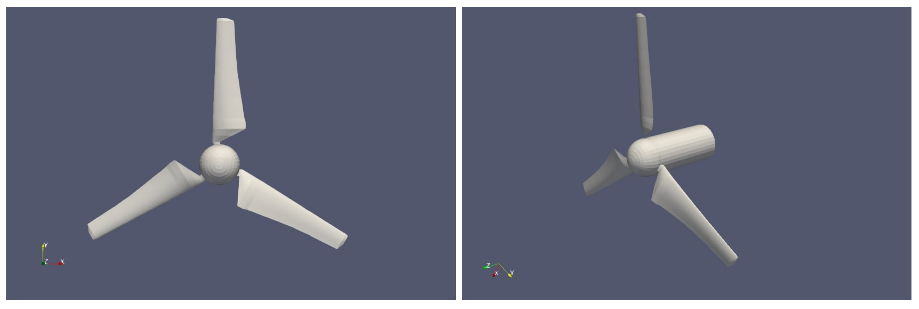
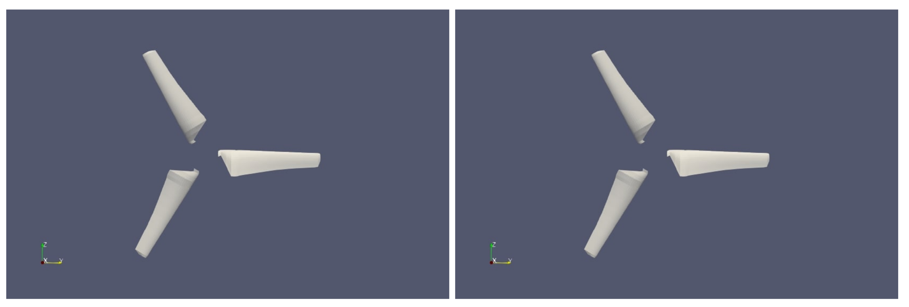
Based on the characteristics of the turbine described in Section 2.1, two geometries were designed. The first one included three blades and a hub in a single volume (Figure 6). The entire turbine was in motion according to [21]’s calculation. This geometry was created in order to obtain comparable results with the experimental data and to enable a comparison between results with and without a hub. Indeed, the mesh around the hub strongly increased the computational cost. Therefore, it was relevant to work without a hub (Figure 7). That is why the second geometry contains only the blades.
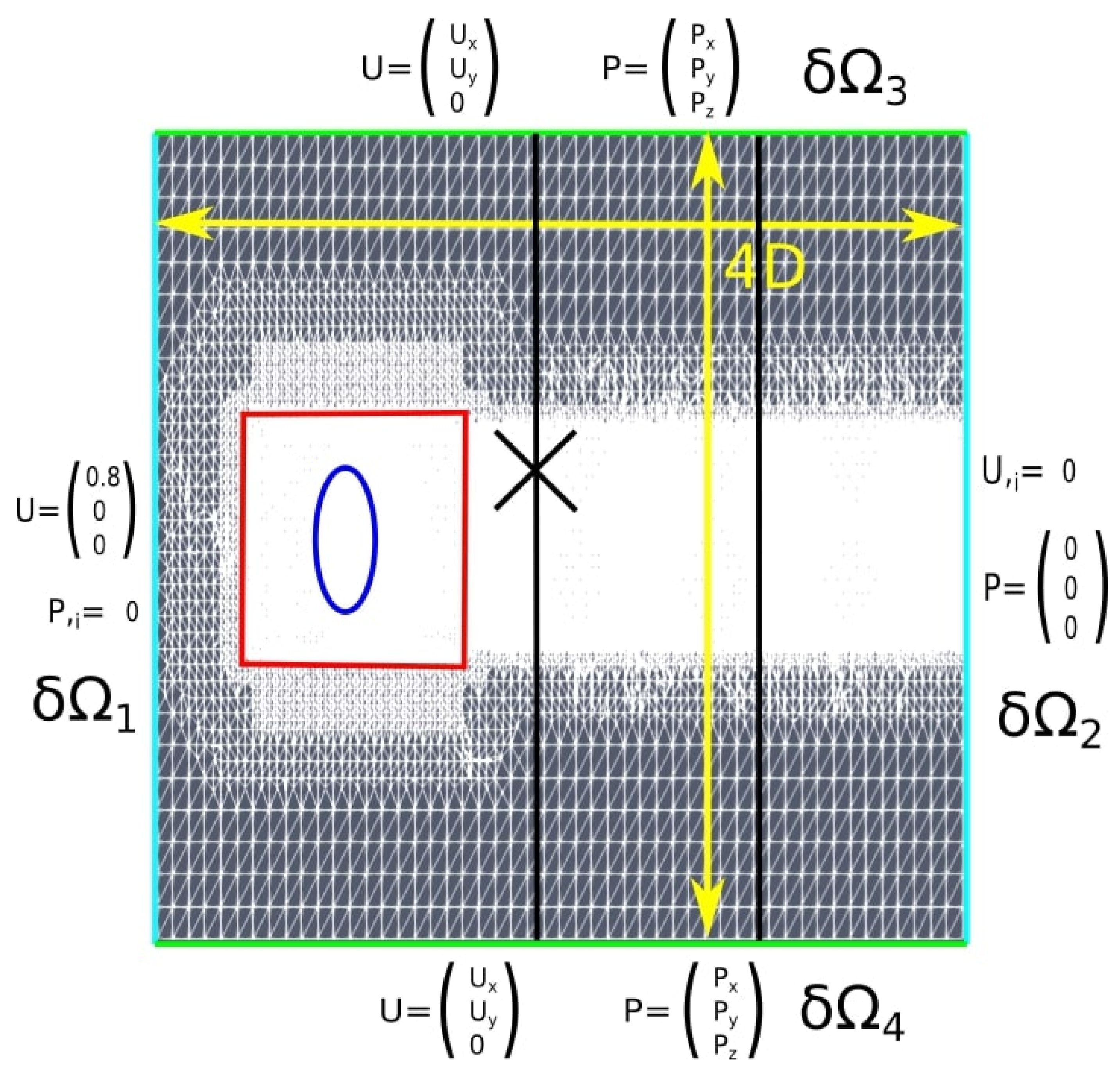
The simulation channel was 4 diameters long and wide. The flow mainly followed the X-axis; thus, the cells were smaller in the X-direction to help respect the CFL condition, ensuring the numerical stability of the code. The mesh behind the rotor was refined to capture the wake (for all the cases except the reference case). The global mesh is shown in Figure 8, where the boundary conditions are reported. As the blades of the IFREMER-LOMC turbine were twisted, the convergence required a finer mesh. For the horizontal axis trial, 5 levels of refinement on the blades were made. Each level was twice smaller than the previous one (Table 1). Level 1 was a cell of in length. The dimensions of the mesh cases are presented in Table 2.
2.3.2. Vertical Axis Turbine
The vertical axis turbine is a Darrieus tidal turbine designed according to the geometry built during the HARVEST program [22] and described in Section 2.1 (Figure 11).
The vertical axis turbine’s mesh was wide and long. The levels were the same as described in the horizontal case. Refinement around the blades was produced using refinement cylinders. Only one mesh was used (Figure 12), but two different motions of the AMI were run: flow-induced and forced motions. The cases are presented in Table 3.
2.4. Numerical Setup
The turbulence intensity was equal to 5% in all the simulations according to the experiment. In all the simulations, the time step was calculated to respect the CFL condition, ensuring the numerical stability of the code for , such that:
where is the maximum velocity magnitude in the domain, is the computing time step in OpenFoam and is the length of the local cell at the position.
The physical parameters of each simulation are described in Table 4 below:
The comparisons between the experimental data and numerical results will be presented using the relative difference, which is expressed for a variable A as:
where is the value of A that is independent of the mesh size.
3. Results and Discussion
3.1. Mesh Convergence
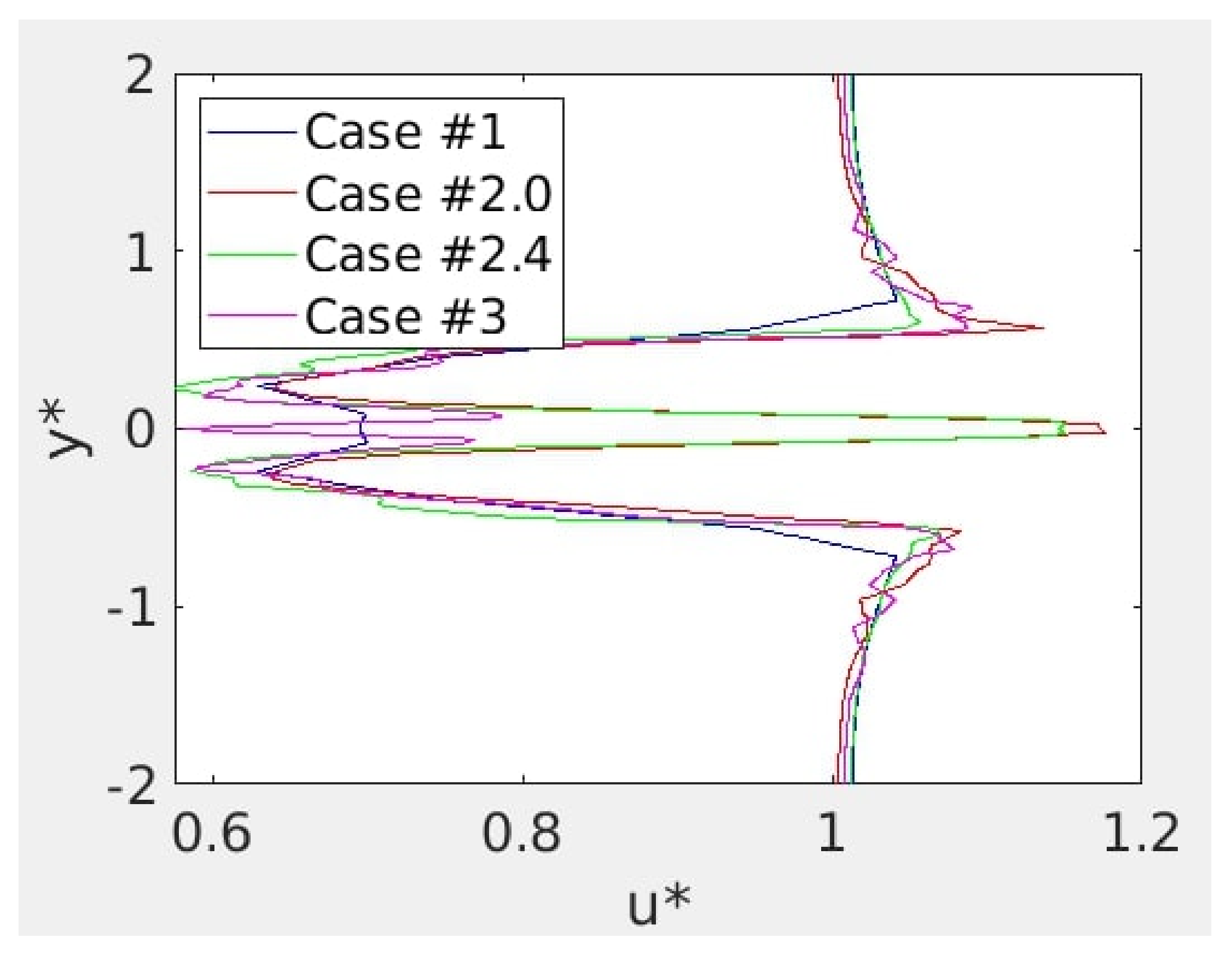
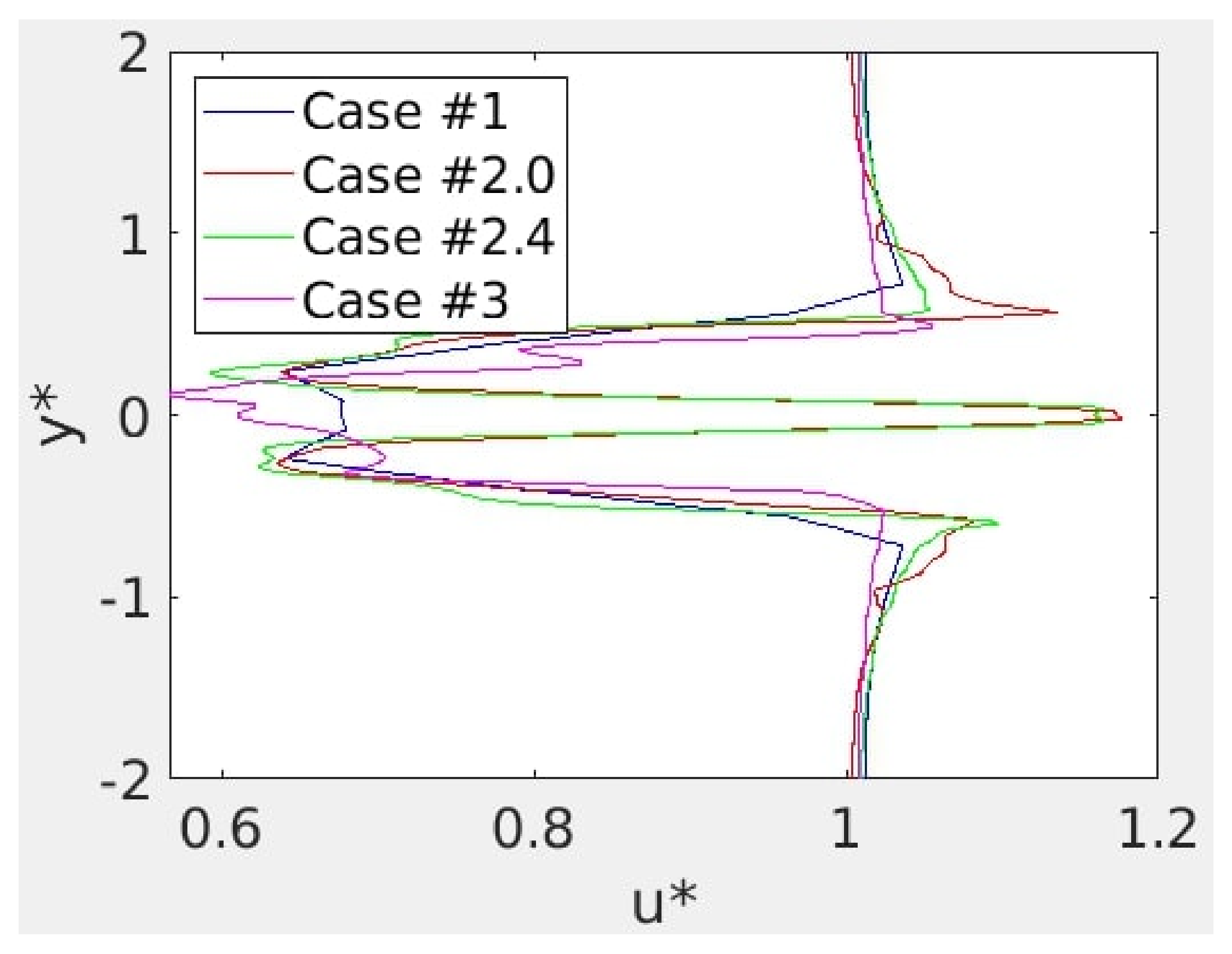
The mesh convergence aimed at ensuring that numerical results were independent from the mesh resolution. The impact of the mesh refinement is first described for the wake before studying it on the blades. Two non-dimensional numbers should be defined: and . The velocity magnitude is compared for different cases in two -positions taken in the plane (Figure 13 and Figure 14). The study was limited to the closest positions of the experimental report because of the short physical time computed due to the very expensive computation time with a 3D grid. All the cases show close results for the minimum values of . However, for the three cases without a hub, the flow accelerated behind where the hub was supposed to be. This effect was reduced when the wake was coarse (case #1), but we observe that it had other significant impacts such as an important loss of the energy in the wake. This phenomenon was due to the size of the filter applied by the Smagorinsky scheme on the coarse mesh.
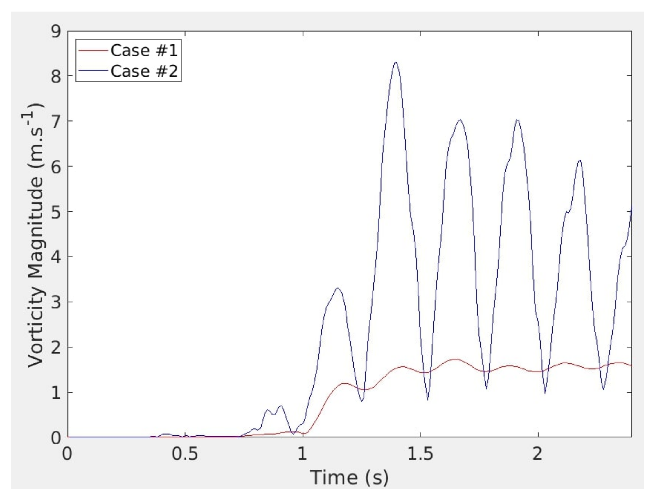
A probe was placed downstream in order to compare the characteristics of the flow. A comparison between cases #1 and #2 shows that the turbulent structures delivered by the rotor, which were exactly the same in the AMI, close to the rotor, were highly dimmed in the wake when the mesh was too coarse (Figure 15). Thus, the level 3 mesh was kept for all the other simulations because it was sufficient for capturing the main turbulent vortexes.
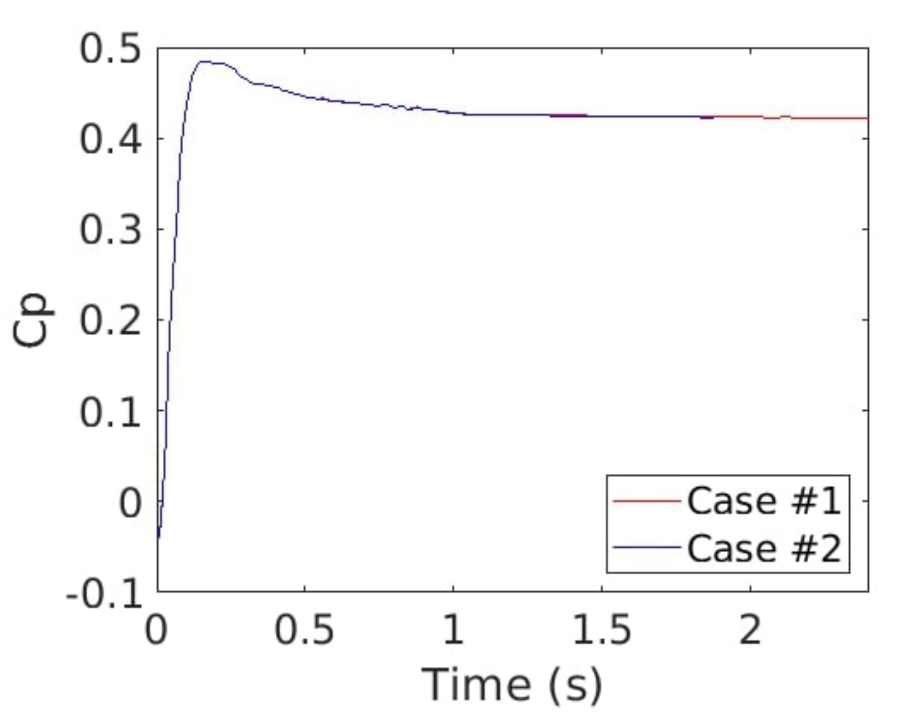
Moreover, as shown in Figure 16, the refinement in the wake did not impact the calculation of the forces applied on the rotor. The refinement in the AMI zone was sufficient, and information from downstream did not impact the upstream flow. As long as the AMI zone is refined and large enough, the wake impact on the performance calculation can be ignored.
Mesh convergence on the blades was performed. Two coefficients—the power coefficient and the drag coefficient , where is the sum of the momentum around the x axis and is the sum of the forces projected in the x direction—were calculated. The values given are the ones reached after coefficient stabilization and averaged for 100 time steps.
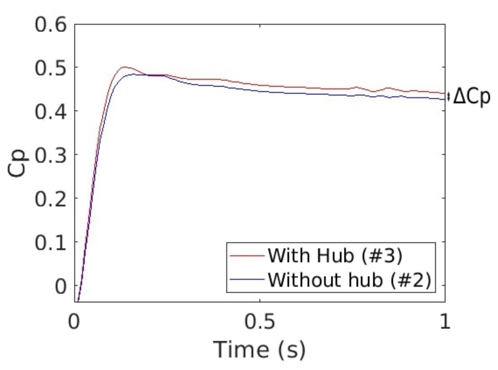
The comparison of cases with and without a hub (Figure 17) shows, as expected, that the removal of the hub implies a drop in the of about 3.6%. A difference in the converged values is noted: . This will be used in Section 3.2.
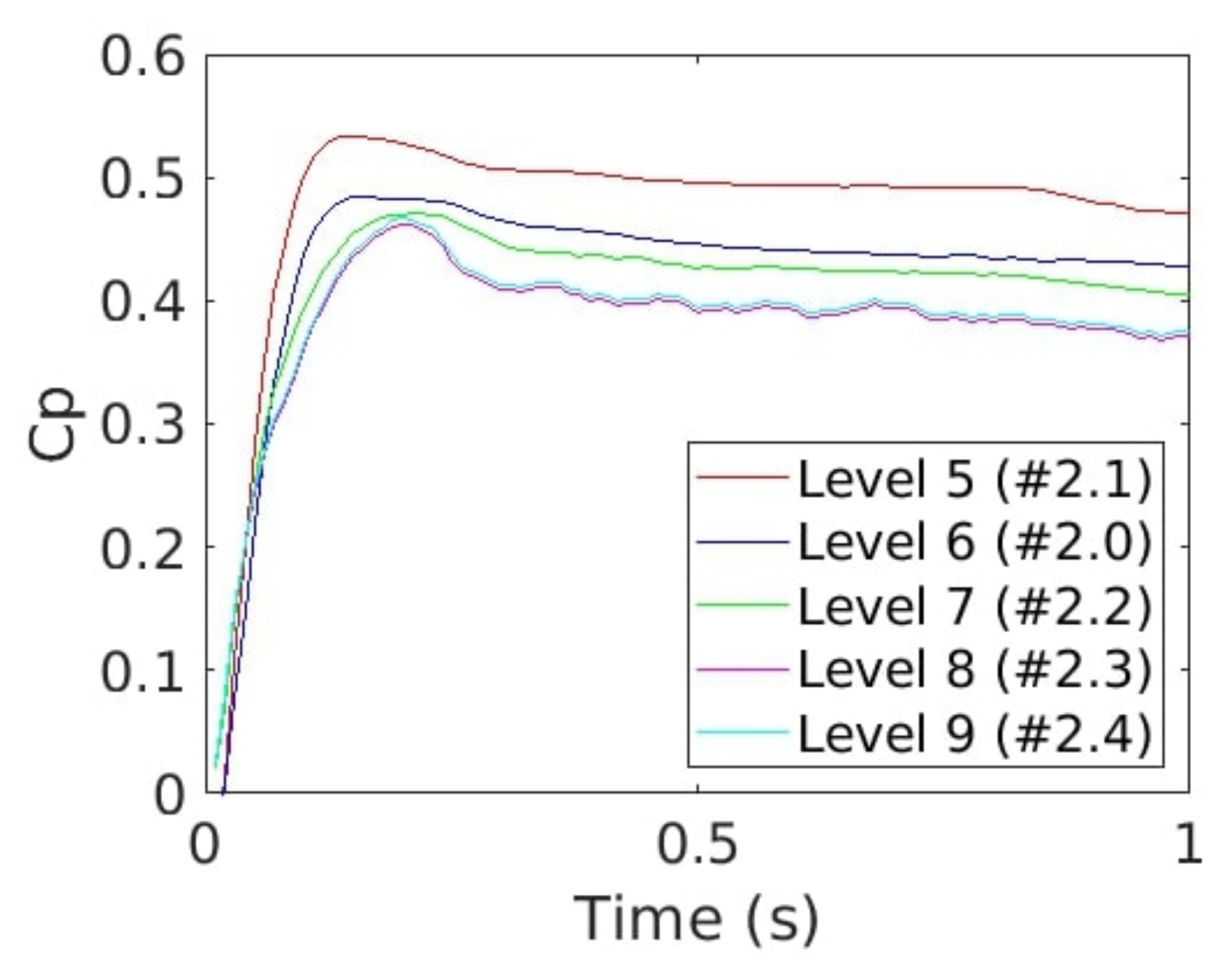
Figure 18 shows the time evolution of Cp for five different levels of refinement on the blades (5 to 9). The model converged after 1 s of physical time. The more the mesh was refined around the blade, the more sensitive it was to flow variations. Coarse meshes gave higher Cps than finer ones. The differences between the various case results were lower when the level increased. The converged values are compared in Table 5.
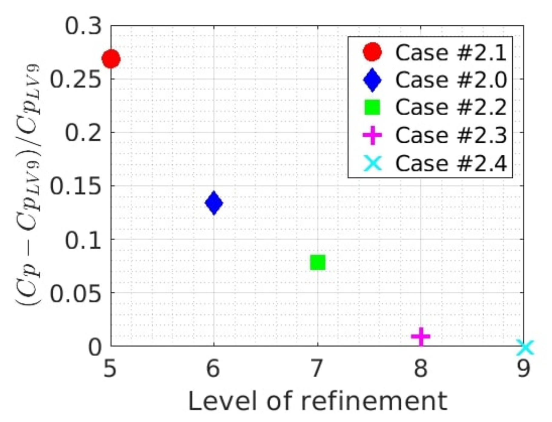
Figure 19 shows that the evolution of the relative difference of Cp compared to the case #2.4 was, as expected, decreasing. The difference between levels 8 and 9 was below 2%. The convergence was reached for a level 8 refinement mesh.
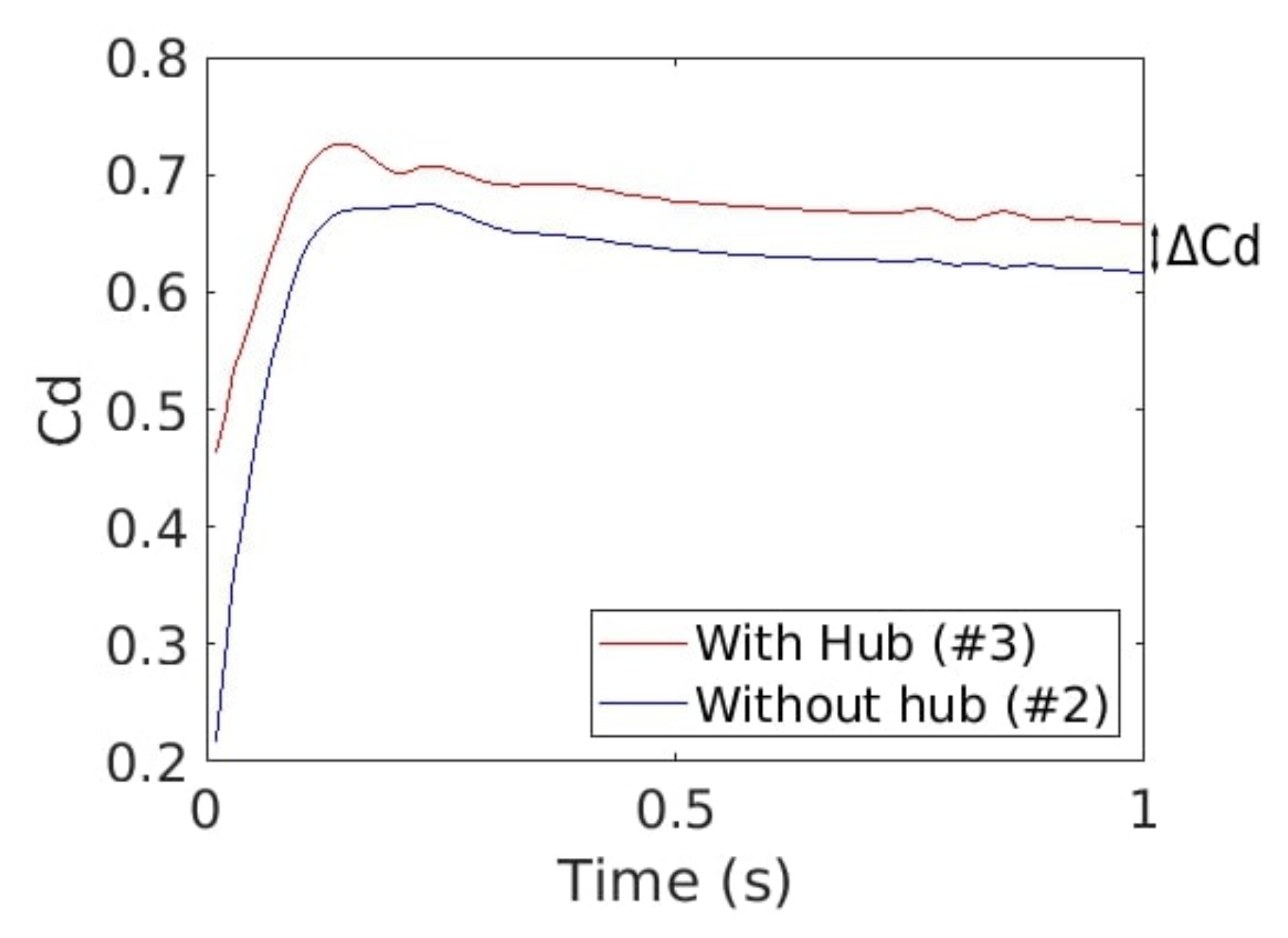
The same method is applied on . The is around (Figure 20). This is low knowing that the hub generates drag.
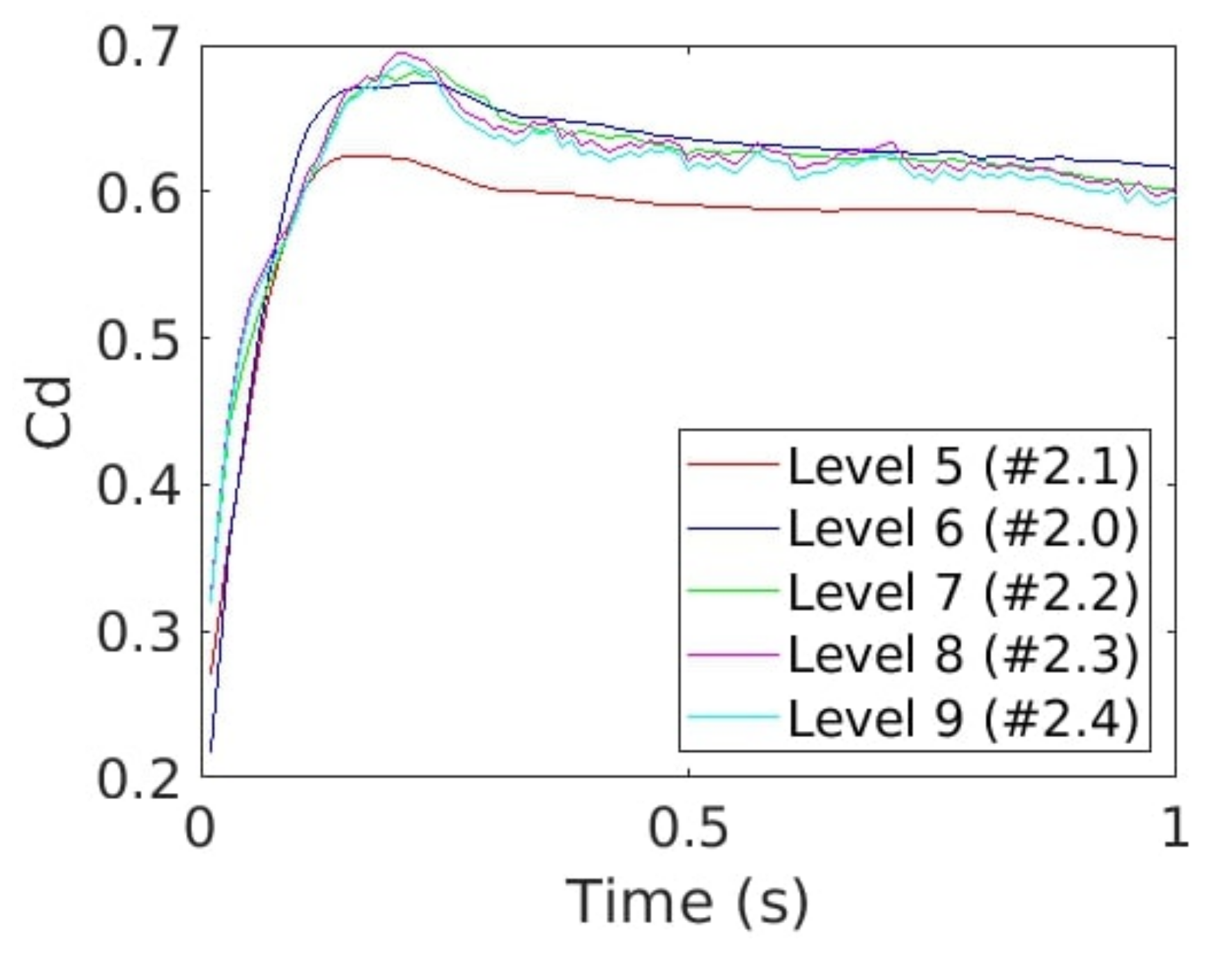
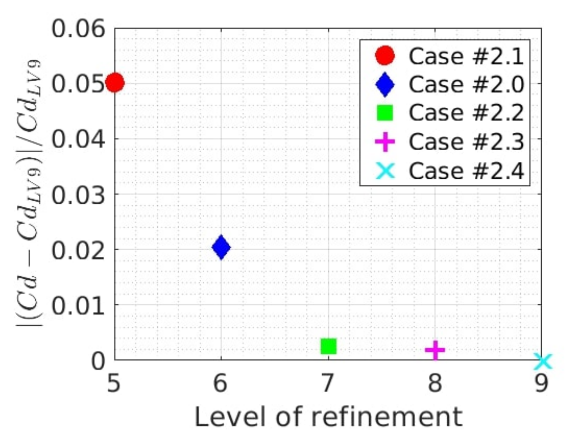
The time evolution of the coefficient (Figure 21) shows really similar results for cases #2.0, #2.2, #2.3 and #2.4. The computed for the case #2.1 is weaker than the other results and case #2.0 slightly above. The solution is stable reaching refinement Level 7. This assertion is confirmed when plotting the relative values of each converged (Figure 22). All the values of coefficients obtained after the time convergence are given in Table 6.
The drag coefficient converged faster than the power coefficient with a stable value from level 7 with a 2% difference between cases #2.2 and #2.4. The and coefficients converged for the level 8 case.
3.2. Validation with Experimental Data
In this section, the testing of the numerical results against the experimental data to validate the model is described.
3.2.1. Horizontal Axis Turbine
The convergence study showed that the solutions of cases #2.3 and #2.4 were close. Thus, we used the results of #2.4 for comparison with the experimental data.
The simulations of the wake were in agreement with the data, with a decrease in the flow velocity due to the turbine with a minimum value at the center of the rotor. Nevertheless, the model seemed to underestimate the energy losses in the wake, particularly near the center of the rotor. This may be due to the high velocity tunnel generated by the missing hub that transfers energy to the surrounding flow. The coefficient was used as a correlation factor such that , where are the experimental data, are the solutions of the simulation and is the mean of the experimental data. This coefficient is usually used for linear function comparisons. It allows us to determine the dispersion between two curves. It was calculated for the results plotted in Figure 23 and Figure 24. The three central data of the velocity profile were removed from the calculation because the acceleration tube was only due to the missing hub. at and at , which is good for this kind of model.
As the study was performed for 3D geometries without a hub, the and were adjusted. This correction was based on the simulations with and without a hub shown in Figure 17 and Figure 20 and discussed in Section 3.1. Thus, the and for the case with a hub were defined as and . The experimental values of and in this configuration were and .
The final results are reported in Table 7:
Despite the solution being independent from the mesh and the hub correction being effective, the model underestimated both coefficients. A possible explanation is the use of a level 6 mesh to estimate the corrections due to the missing hub not being sufficient. Our computing resources do not allow running simulations with a finer mesh and hub. The difference could also have come from the experimental conditions, where the flume was smaller than the numerical one, which could have generated side effects affecting the data.
3.2.2. Vertical Axis Turbine
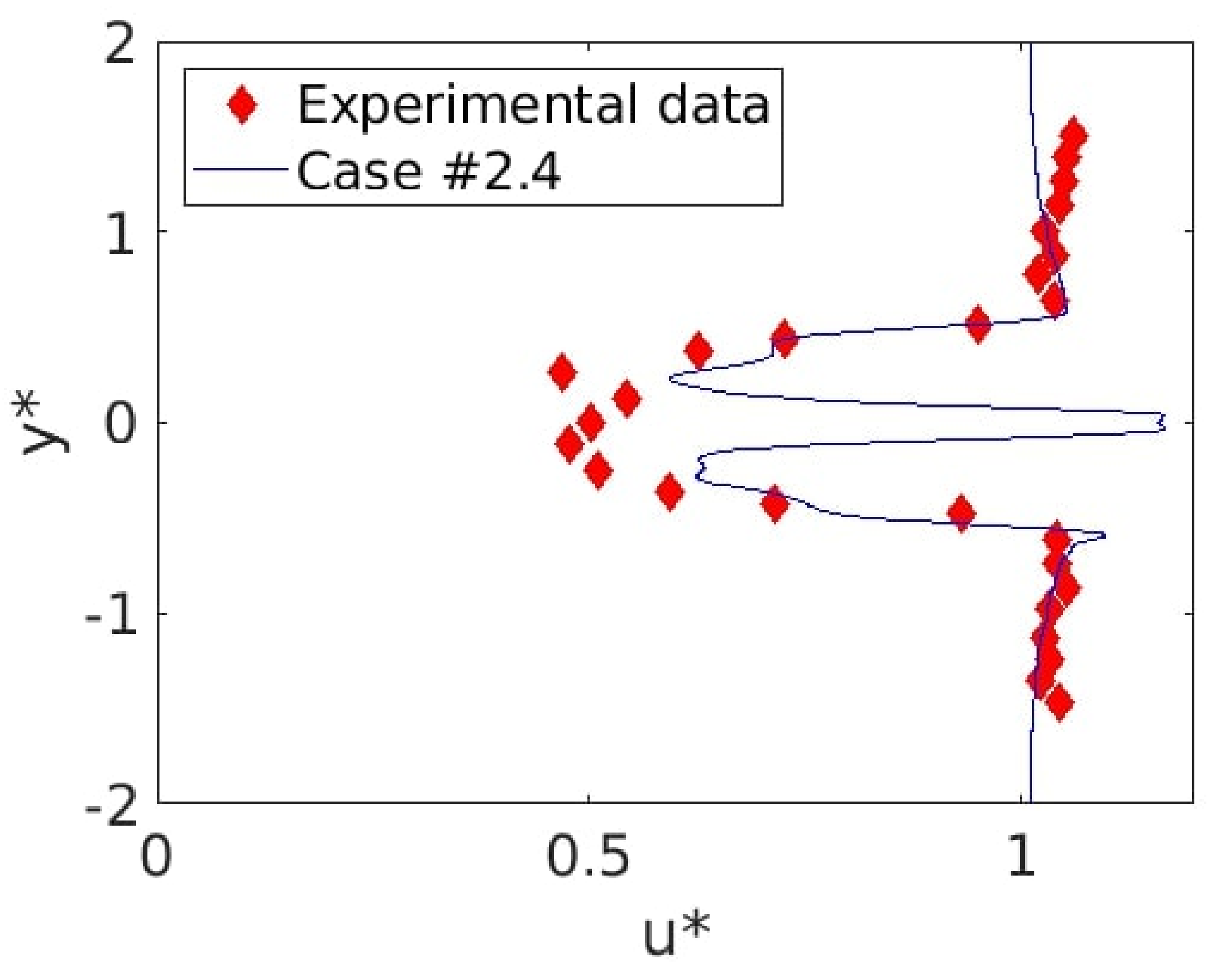
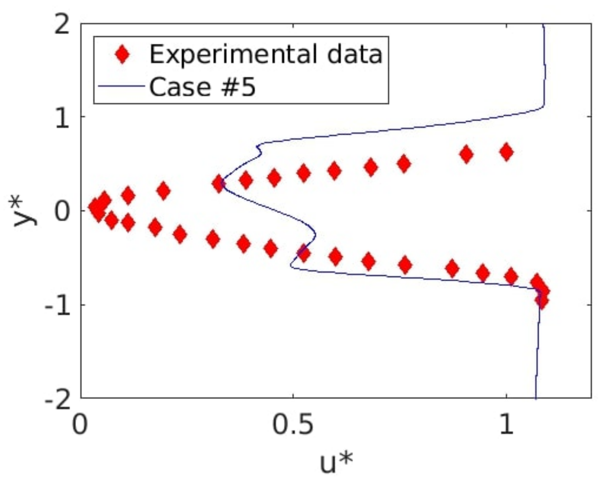
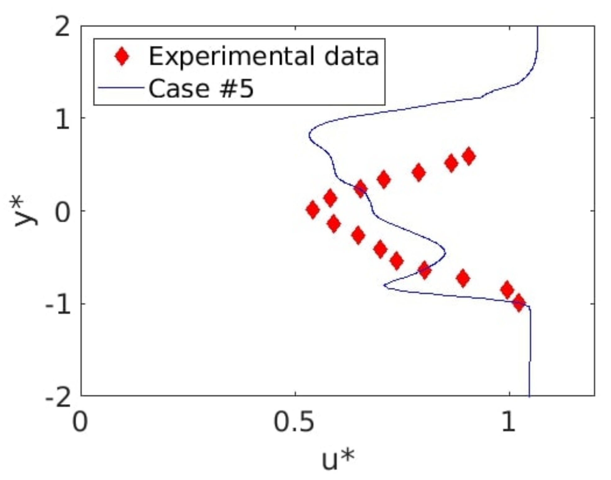
The vertical axis geometry was made with straight blades. This implies that it was easier to capture the structure within the code. Nevertheless, the horizontal axis turbine rotated faster than the horizontal one. The forces applied on the blades and the wake were more chaotic. Figure 25 and Figure 26 show the time-averaged (over 1.5 s) non-dimensional speed in the wake, in 2D and 4D, behind the turbine. The averaging was performed once the flow was settled. The model seemed to underestimate the energy losses near the rotor, but this effect was decreased downstream. This difference may be due to the lack of a hub and transverse blades in the model, but the null velocity downstream for the turbine in the experimental data can also be discussed. at and at . These low values can be explained by the shift between the data and numerical results.
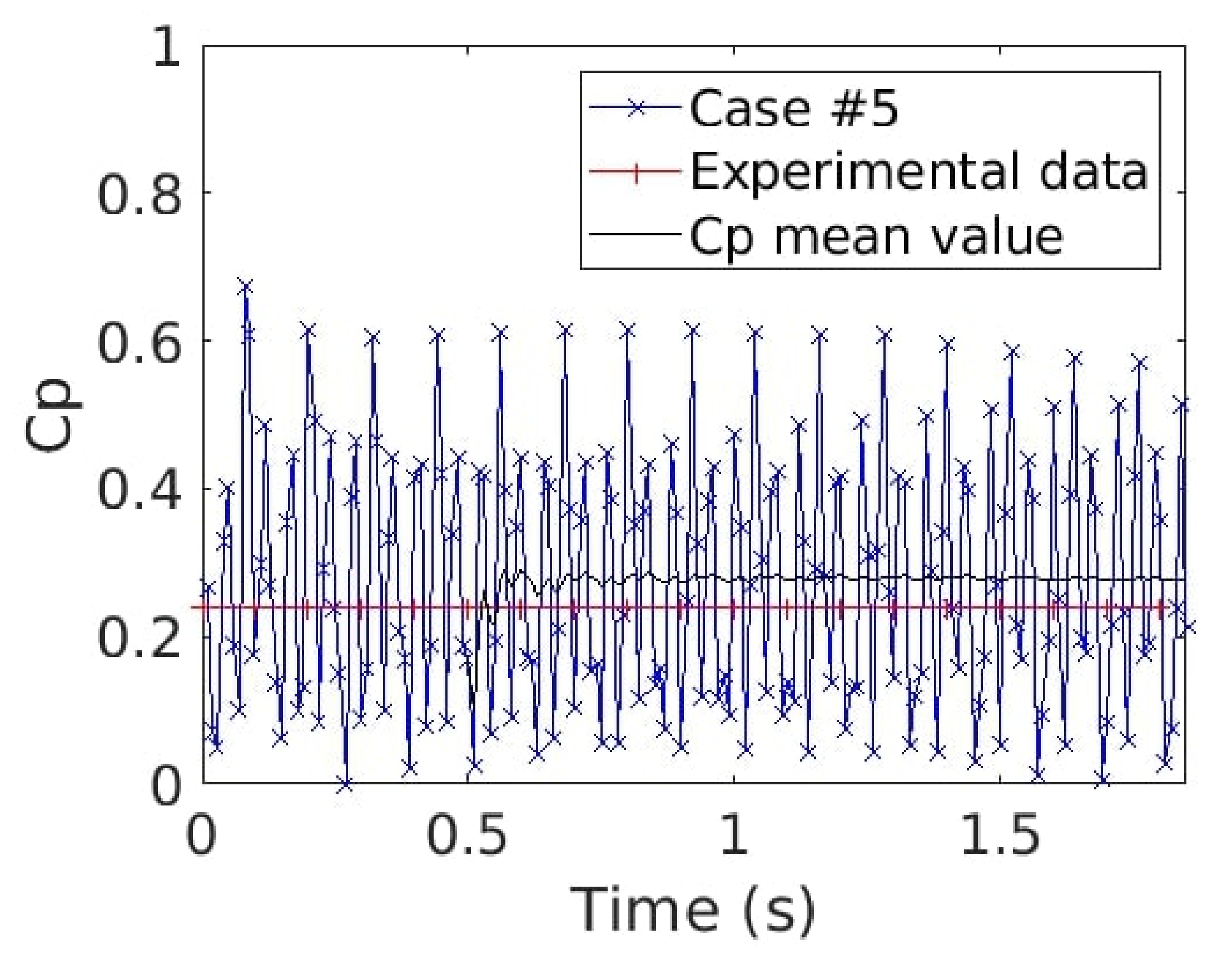
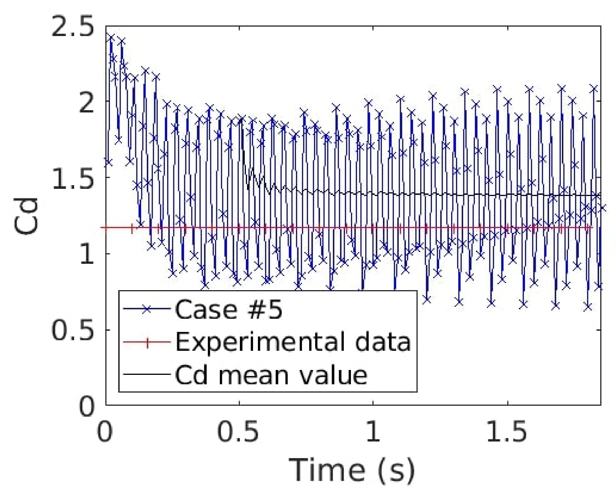
Due to the high-velocity rotation, the on the blades varied very rapidly. As shown in Figure 27 and Figure 28, the values did not directly converge but oscillated around a value that evolved in time. This is why once the signal stabilized, the average was taken on the last values to evaluate the mean coefficients. The results are given in Table 8. The error in this case is greater than the one on the horizontal axis. This is due to the relatively coarse mesh. However, Section 3.3 shows that the mesh refinement does not change the solution of flow-induced simulations in free rotation.
3.3. Flow-Induced Model Validation
The lack of experimental data is critical when validating flow-induced models. As explained before, it is widespread to force the rotation with a motor in experimental approaches. The free rotation speed value cannot be determined with certainty, but owing to the mesh convergence study (see Section 3.1), we know that the model is adequate for estimating forces in forced rotation cases. There are two ways to check the model validity. Firstly, the time evolution of the rotor speed. As long as the motion is computed only using the fluid forces, the direction of rotation and the rotor acceleration are parameters to be monitored. The total mass of each solid geometry was calculated based on its density, fixed to the fluid density to avoid the Archimedean thrust effects. Then, for each free speed case, an equivalent forced case was created. The speed of the forced rotation simulations was the one reached by the free case. The signals in the wake were compared. If the signals matched, the implantation of the flow-induced rotation did not change the behavior of the fluid solver. This validation method was applied on the vertical and the horizontal axis simulations.
3.3.1. Free Horizontal Tidal Turbine
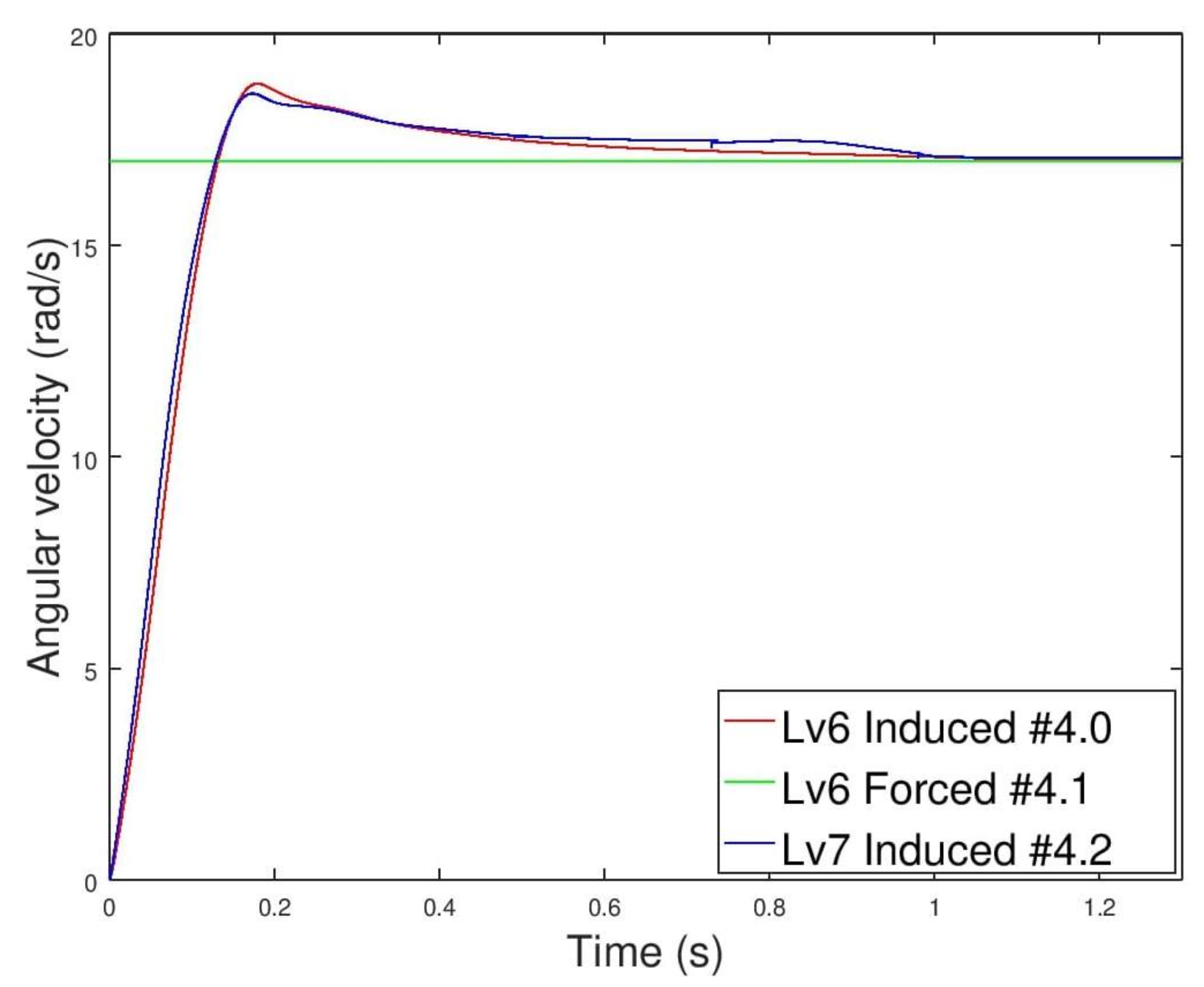
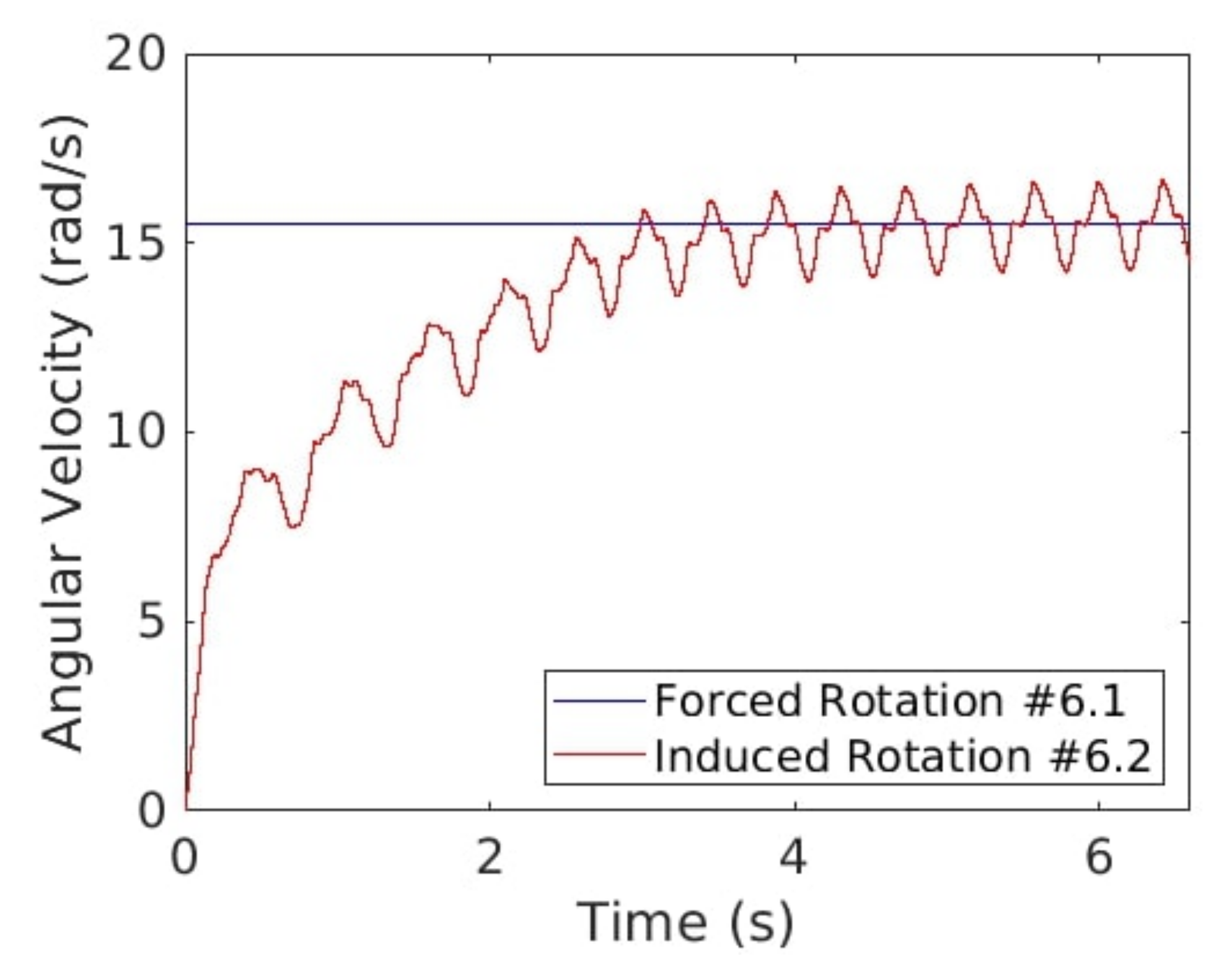
For the horizontal axis turbine, three cases are compared (#4.0, #4.1 and #4.2). The two first cases were built with a level 6 refinement on the blades. Case #4.0 was a free flow-induced simulation. As presented in Figure 29, the rotational speed quickly converged to . The direction of the rotation was consistent with the blade orientation: as we let the turbine rotate freely, it is important that the turbine rotation matches reality. Case #4.1 used the same mesh as #4.1, but the rotation speed was fixed to the final rotation speed of case #4.0. Case #4.2 was a free flow-induced case but with a finer mesh on the blades (twice smaller). The angular velocities for each case are plotted in Figure 29. For the two flow-induced cases, the curves passed through two distinct phases. The acceleration phase was short, less than . After reaching a maximum, the angular velocity slowly stabilized around its final value. In this type of trial, we were expecting that the final value would be the global maximum of the curve. The overtaking can be explained by the fact that the code needs to compute numerous time steps to convert the acceleration into speed. This method was used to ensure the stability of the code. The angular speed behavior for #4.0 and #4.2 was the same. The final value towards which the code converged was very close in both cases. The mesh refinement for one of the blades seemed to have a weak effect on the rotation speed results. Case #4.1 was a forced case using the converged rotation speed as the inlet velocity.
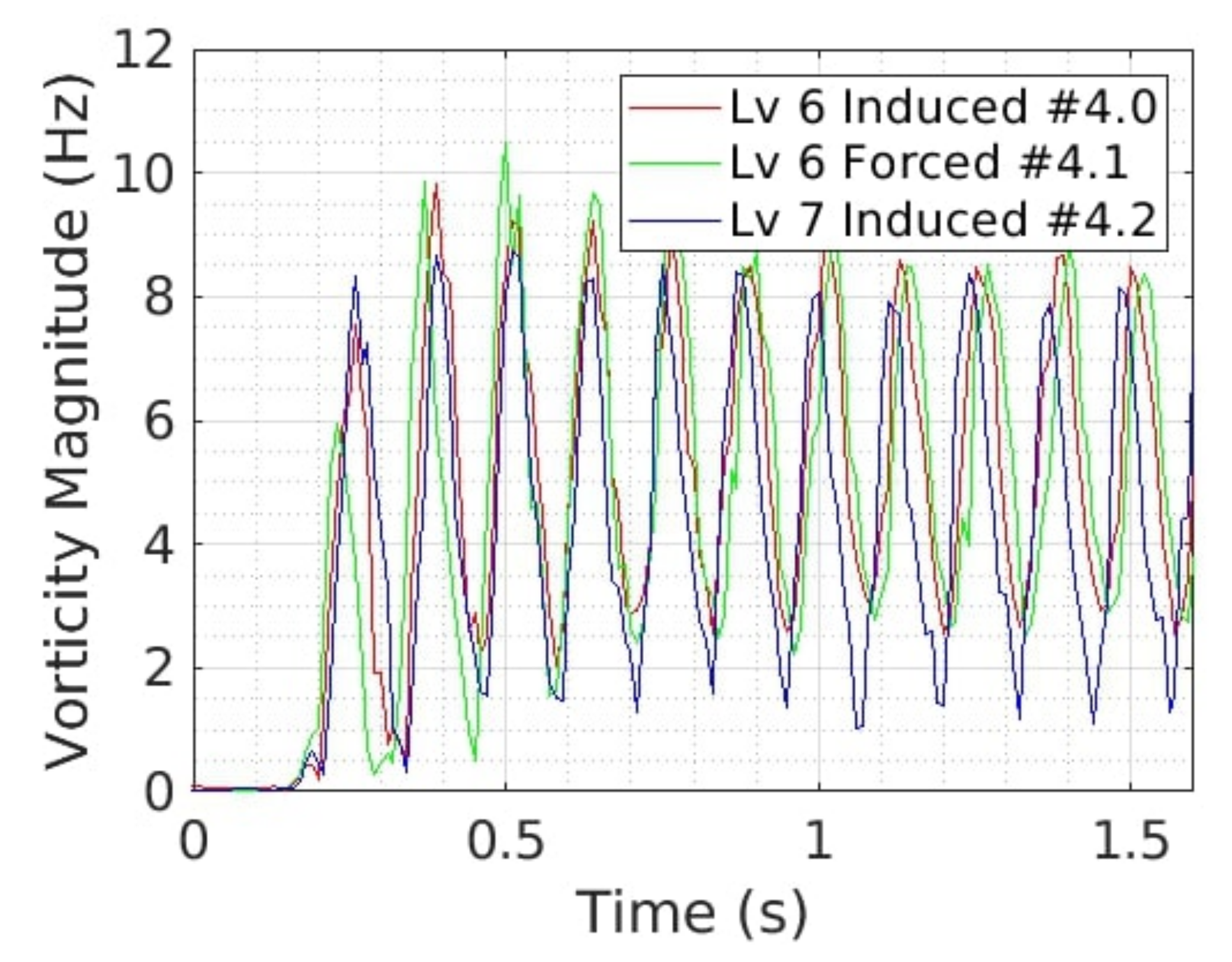
In order to study the impact of the flow-induced rotation on the fluid motion, a numerical probe was placed down the flow one diameter downstream of the turbine in the tip of the blade wake. Figure 30 shows the vorticity magnitude over time at the probe location. The three cases had similar behaviors. The signals were also a bit shorter in case #4.2 than in case #4.0. A phase shift is observed between case #4.1 and the two others. It is due to the acceleration phase of the rotor in the flow-induced simulations. Once the shift was corrected by removing the time steps corresponding to the acceleration phase, the signals of the three cases were very close (Figure 30). However, we can observe a small variation of the amplitude between cases #4.0 and #4.2. The mesh refinement on the blades slightly changed the vortex generation, and a finer mesh allowed capturing smaller vortical structures.
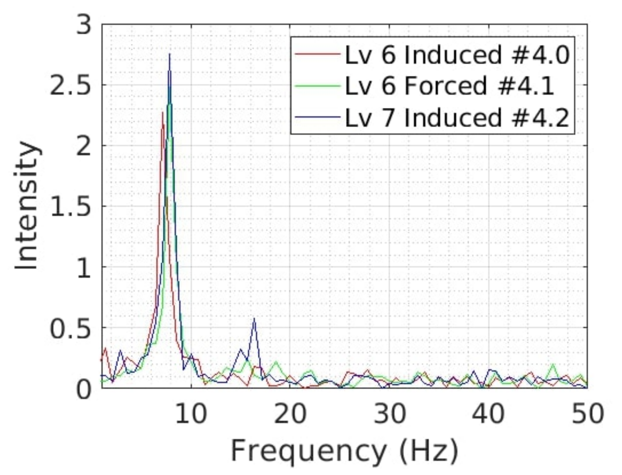
To check if the signal was definitely the same, a fast Fourier transform was applied for the stabilized period from 0.3 to 1.6 s (Figure 31). For the horizontal axis turbine, the signal had a primary peak around 7.8 . This peak corresponded to the passage of a tidal turbine blade upstream. The mesh refinement on the blades barely impacted the wake signal.
3.3.2. Free Vertical Tidal Turbine
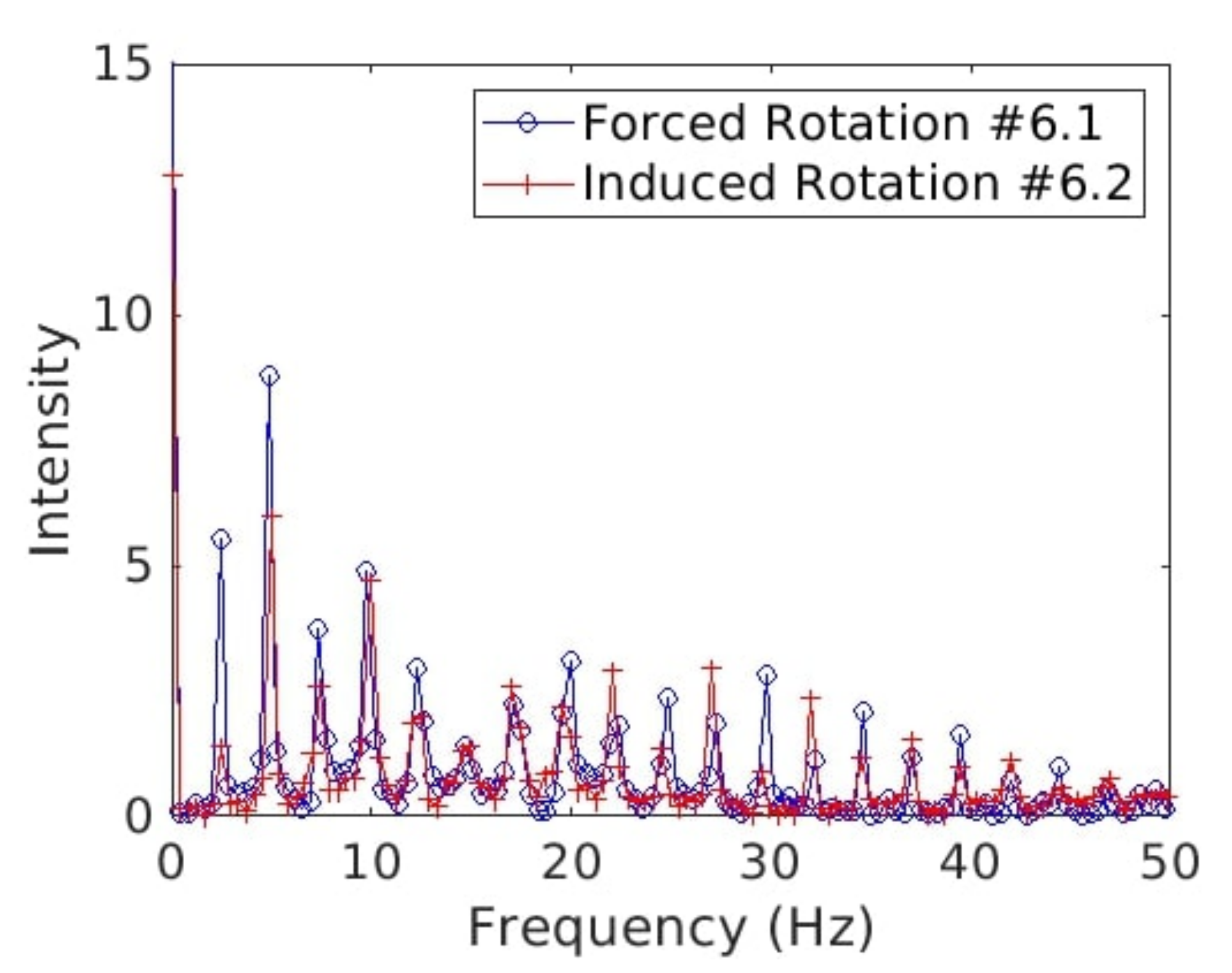
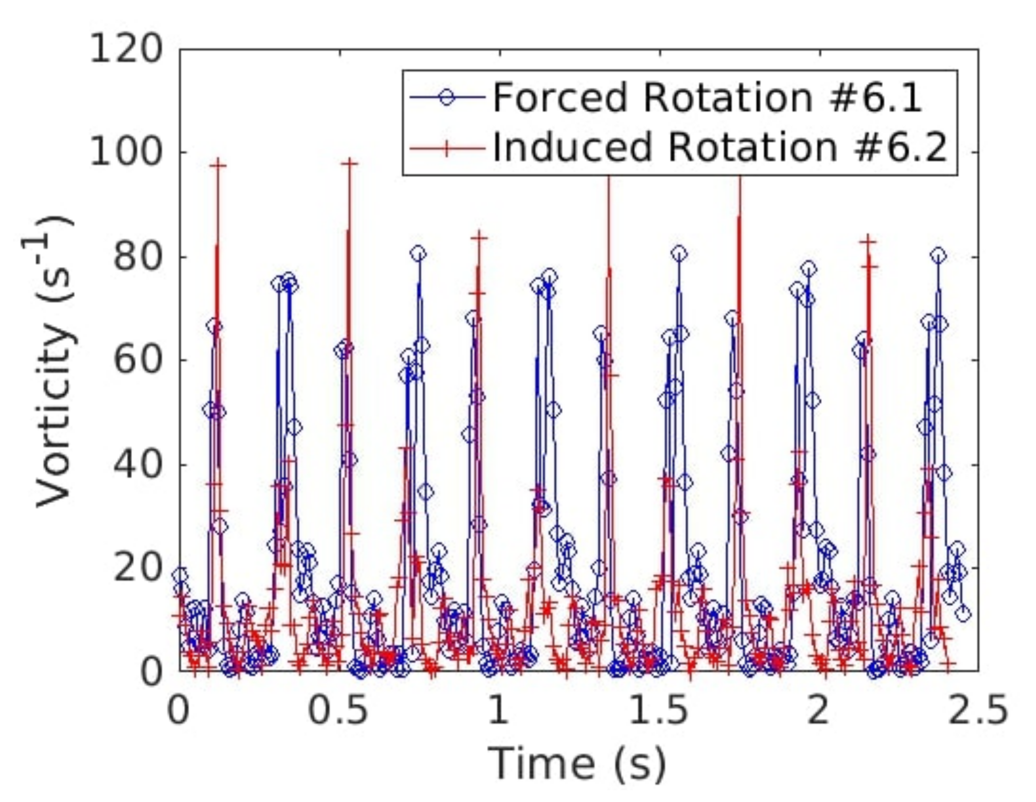
The same methodology was used for the vertical axis turbine. The final free flow-induced angular velocity averaged on two full rotations reached 15.5 . Unlike that for the horizontal axis turbine, the flow-induced angular velocity signal contained peaks. They were due to the effect of the upflow blade on the two others through the generated vortexes (Figure 32). Because of this, the signal in the wake contained a lot more harmonics than the signal of the horizontal axis turbine (Figure 33). The difference in the harmonics intensity was due to the acceleration/deceleration phases in the flow-induced case. It was more difficult to analyze the signal of the vertical axis turbine because of the interactions between the blades through the fluid. However, the main frequencies were conserved between the forced and flow-induced cases, with a primary peak around 4 Hz. Once again, the flow-induced rotation did not seem to disturb the fluid solution as shown in Figure 34.
4. Conclusions
In this paper, a numerical study for horizontal and vertical axis tidal turbines was carried out. Simulations showed that the results were sensitive to mesh precision. After reaching a level 8 refinement, the solution became independent of the mesh resolution. The level of refinement varied with the size of the turbulent structures that we wanted to simulate. To study the performance of a turbine, a finer refinement should be applied near the blades. It becomes useless to have a fine mesh in the wake if the only goal of the study is to predict the turbine’s performance. Nevertheless, a coarse mesh does not allow capturing small-size fluid structures in the wake. The comparison with experimental data shows that our model underestimated the energy losses in the wake as well as the and , but the error did not exceed 10% for the converged mesh case. The results given by a relatively coarse mesh are still better than a 2D simulation [28] for performance and far-field wake predictions. This may be due to the fact that 3D simulations capture the tip vortexes that have a strong effect on the performance and the wake behavior.
A flow-induced rotation approach is also presented. The results were compared to equivalent forced rotation to assess their coherence. The rotor behavior was consistent with the free turbines turning in the correct direction at a very high rotational speed. The lack of experimental data for turbine free rotation is a limitation to completely validating the model. Nevertheless, flow-induced rotation code cannot be used in this format: a brake should be implemented to model the energy recuperation and the control system of the turbine. Then, it would be possible to study both the turbine performance, directly based on its energy production, and its starting phase. We could also predict the amount of electricity produced as a function of the flow and rotor speeds using an energy conversion model. The rotor speed would be controlled by the brake’s power. Once this step has been reached, a new comparison with “forced rotation” cases could be made for validation. Flow-induced rotation will help in studying the impact of mass variation (due to a change in the turbine material or fouling by organisms such as barnacles and mussels on the rotor, i.e., their settlement on the rotor and their numbers) on the starting phase. However, that will also be useful for developing a new type of turbine that could start with a low flow speed, by studying the starting phase and the performance at the same time. Prototype turbines with vertical axes and variable diameters are currently being developed, and we believe that our approach could be used before the scale models are built.
Author Contributions
Conceptualization, I.R. and A.-C.B.; Methodology, I.R. and A.-C.B.; Software, I.R.; Investigation, I.R., A.-C.B.; Writing–Original Draft Preparation, I.R.; Writing–Review & Editing, I.R., A.-C.B. and J.-C.D.; Supervision, A.-C.B. and J.-C.D.; Funding Acquisition, A.-C.B. and J.-C.D. All authors have read and agreed to the published version of the manuscript.
Funding
The research was supported by the “Région Normandie” through a PhD grant (no grant number) and by the “Université de Caen Normandie” (no grant number).
Institutional Review Board Statement
Not applicable.
Informed Consent Statement
Not applicable.
Data Availability Statement
The author will provide OpenFoam files and result data on request.
Acknowledgments
The authors are grateful to the CRIANN for the calculation facilities and technical support. We thank Patrice Robin for his English revision.
Conflicts of Interest
The authors declare no conflict of interest. The funders had no role in the design of the study; in the collection, analyses, or interpretation of data; in the writing of the manuscript; or in the decision to publish the results.
Abbreviations
| Parameters | Definitions | Units |
| D | Rotor diameter | |
| R | Rotor radius | |
| Computational domain inlet surface | - | |
| Computational domain outlet surface | - | |
| Computational domain side surfaces | - | |
| Surface normal vector | - | |
| Surface normal vector in the blade referential | - | |
| Surface tangential vector in the blade referential | - | |
| Kinematic viscosity | ||
| Rotor angular velocity | ||
| Computational domain | - | |
| p | Fluid pressure | |
| Fluid density | ||
| Inlet velocity magnitude | ||
| Tip speed ratio |
References
- Eurel, K.; Sullivan, P.; Gleason, M.; Hettinger, D.; Heimiller, D.; Lopez, A. An Improved Global Wind Resource Estimate for Integrated Assessment Models. Energy Econ. 2019, 64, 552–567. [Google Scholar]
- Raoux, A.; Tecchio, S.; Pezy, J.; Lassalle, G.; Degraer, S.; Wilhelmson, D.; Cachera, M.; Ernande, B.; Le Guen, C.; Haraldsson, M.; et al. Benthic and fish aggregation inside an offshore wind farm: Which effects on the trophic web functioning? Ecol. Indic. 2019, 72, 33–46. [Google Scholar] [CrossRef] [Green Version]
- Weiss, C.; Guanche, R.; Ondiviela, B.; Castellanos, O.; Juanes, J. Marine renewable energy potential: A global perspective for offshore wind and wave exploitation. Energy Convers. Manag. 2018, 177, 43–54. [Google Scholar] [CrossRef]
- Encarnacion, J.; Johnstone, C.; Ordonez-Sanchez, S. Design of a Horizontal Axis Tidal Turbine for Less Energetic Current Velocity Profiles. J. Mar. Sci. Eng. 2019, 7, 197. [Google Scholar] [CrossRef] [Green Version]
- Euler, L. Principes généraux du mouvement des fluides. Mémoires de l’Académie des Sciences de Berlin 1757, 11, 274–315. [Google Scholar]
- Lee, C.; Kim, B.; Kim, N. A simple lagrangian PDF model for wall-bounded turbulent flows. KSME Int. J. 2000, 14, 900–911. [Google Scholar] [CrossRef]
- Mycek, P.; Pinon, G.; Lothodé, C.; Dezotti, A.; Carlier, C. Iterative solver approach for turbine interactions: Application to wind or marine current turbine farms. Appl. Math. Model. 2017, 41, 331–349. [Google Scholar] [CrossRef] [Green Version]
- Hansen, M.; Sorensen, J.; Michelsen, J.; Sorensen, N. A global Navier-Stokes rotor prediction model. In Proceedings of the 35th Aerospace Sciences Meeting and Exhibit, Reno, NV, USA, 6–9 January 1997. [Google Scholar]
- Liu, Y.; Xiao, Q.; Incecik, A.; Peyrard, C.; Wan, D. Establishing a fully coupled CFD analysis tool for floating offshore wind turbines. Renew. Energy 2017, 112, 280–301. [Google Scholar] [CrossRef] [Green Version]
- Osbourne, N.; Groulx, D.; Penesis, I. Three dimensional simulation of a horizontal axis tidal turbine—Comparison with experimental results. In Proceedings of the 2nd Asian Wave and Tidal Energy Conference (AWTEC), Tokyo, Japan, 27–30 July 2014. [Google Scholar]
- Antheaume, S.; Maître, T.; Achard, J.-L. Hydraulic Darrieus turbines efficiency for free fluid flow conditions versus power farms conditions. Renew. Energy 2008, 33, 2186–2198. [Google Scholar] [CrossRef]
- Rivier, A.; Bennis, A.C.; Jean, G.; Dauvin, J.C. Numerical simulations of biofouling effects on the tidal turbine hydrodynamic. Int. Mar. Energy J. 2018, 1, 101–109. [Google Scholar] [CrossRef]
- Abdul Rahman, A.; Venugopal, V.; Thiebot, J. On the Accuracy of Three-Dimensional Actuator Disc Approach in Modelling a Large-Scale Tidal Turbine in a Simple Channel. Energies 2018, 11, 2151. [Google Scholar] [CrossRef] [Green Version]
- Vogel, C.; Willden, R.; Houlsby, G. Blade element momentum theory for a tidal turbine. Ocean Eng. 2018, 169, 215–226. [Google Scholar] [CrossRef]
- Dumitrescu, H.; Cardos, V. Wind Turbine Aerodynamic Performance by Lifting Line Method. Int. J. Rotating Mach. 1998, 169, 141–149. [Google Scholar] [CrossRef] [Green Version]
- Grondeau, M.; Guillou, S.; Mercier, P.; Poizot, E. Wake of a Ducted Vertical Axis Tidal Turbine in Turbulent Flows, LBM Actuator-Line Approach. Energies 2019, 12, 4273. [Google Scholar] [CrossRef] [Green Version]
- Song, S.; Demirel, Y.K.; Atlar, M.; Shi, W. Prediction of the fouling penalty on the tidal turbine performance and development of its mitigation measures. Appl. Energy 2020, 276, 115498. [Google Scholar] [CrossRef]
- Devolder, B.; Schmitt, P.; Rauwoens, P.; Elsäßer, B.; Troch, P. A Review of the Implicit Motion Solver Algorithm in OpenFOAM to Simulate a Heaving Buoy. In Proceedings of the 18th Numerical Towing Tank Symposium, Marstrand, Sweden, 28–30 September 2015. [Google Scholar]
- Srivastava, A.; Akhtar, H.; Gupta, A.; Kumar, R. Hydrodynamic Analysis of the Ship Hull. Int. J. Emerg. Technol. Eng. Res. 2019, 4, 25–28. [Google Scholar]
- Guo, X.; Gao, Z.; Li, X.; Yang, J.; Moan, T. Loading and Blade Deflection of a Tidal Turbine in Waves. Offshore Mech. Arct. Eng. 2019, 141, 041902. [Google Scholar] [CrossRef]
- Mycek, P. Numerical and Experimental Study of the Behaviour of Marine Current Turbines. Ph.D. Thesis, University of Le Havre, Le Havre, France, 2013. [Google Scholar]
- Menchaca Roa, A. Numerical Analysis of Vertical Axis Water Current Turbines Equipped with a Channelling Device. Ph.D. Thesis, University of Grenoble, Saint-Martin-d’Hères, France, 2011. [Google Scholar]
- Kiho, S.; Shiono, M.; Suzuki, K. The power generation from tidal currents by darrieus turbine. Renew. Energy 1996, 9, 1242–1245. [Google Scholar] [CrossRef]
- Smagorinsky, J. General circulations experiments with the primitive equations. Mon. Weather Rev. 1963, 91, 99–164. [Google Scholar] [CrossRef]
- Katopodes, N. Chapter 8—Turbulent Flow. In Free-Surface Flow; Environmental Fluid Mechanics; Butterworth-Heinemann: Oxford, UK, 2019; pp. 540–615. [Google Scholar]
- Greenshields, C. OpenFoam User Guide, Version 6; OpenFOAM Foundation, 2018. Chapter 3.5. Available online: https://cfd.direct/openfoam/user-guide/v8-standard-solvers/ (accessed on 12 December 2020).
- Marten, D.; Peukert, J.; Pechlivanoglou, G.; Nayeri, C.; Paschereit, C. QBLADE: An Open Source Tool for Design and Simulation of Horizontal and Vertical Axis Wind Turbines. Int. J. Emerg. Technol. Adv. Eng. 2013, 3, 264–269. [Google Scholar]
- Delafin, P.L.; Guillou, S.; Sommeria, J.; Maitre, T. Mesh sensitivity of vertical axis turbine wakes for farm simulations. In Proceedings of the Congrès Français de Mécanique, Brest, France, 26–30 August 2019. [Google Scholar]
Figure 1.
General characteristics (a) and design (b) of the IFREMER-LOMC turbine [21], University of Le Havre, 2013.
Figure 1.
General characteristics (a) and design (b) of the IFREMER-LOMC turbine [21], University of Le Havre, 2013.

Figure 2.
Geometry of the Darrieus tidal turbine [22], University of Grenoble, 2011.
Figure 2.
Geometry of the Darrieus tidal turbine [22], University of Grenoble, 2011.

Figure 3.
Scheme of one iteration of PimpleFoam performed and repeated until the reaching of the convergence criteria. and are, respectively, the estimate of the velocity matrix and pressure matrix. and are the corrected pressure and velocity fields at iteration n.
Figure 3.
Scheme of one iteration of PimpleFoam performed and repeated until the reaching of the convergence criteria. and are, respectively, the estimate of the velocity matrix and pressure matrix. and are the corrected pressure and velocity fields at iteration n.

Figure 4.
and for a blade profile (red line).

Figure 5.
Energy recovery chain for real life (red box), the forced rotation (blue box) and the flow induced rotation (green box). Black arrows represent the energy transfer.
Figure 5.
Energy recovery chain for real life (red box), the forced rotation (blue box) and the flow induced rotation (green box). Black arrows represent the energy transfer.

Figure 6.
Three-dimensional views of the horizontal tidal turbine with a hub: front (left panel) and sideways (right panel) views.
Figure 6.
Three-dimensional views of the horizontal tidal turbine with a hub: front (left panel) and sideways (right panel) views.

Figure 7.
Same legend as for previous figure but without a hub.

Figure 8.
View of the X–Y plane of the computational domain with boundary conditions. D is the rotor diameter. U is the flow velocity in , P is the pressure in , and is the pressure at the calculated point closest to the wall. The red square delimits the arbitary mesh interface (AMI) zone, and the blue circle shows the rotor position. The two black lines (1.2D and 2D) and the black cross are the extraction lines and the probe, respectively, used in the model validation in Section 3.2.

Figure 9.
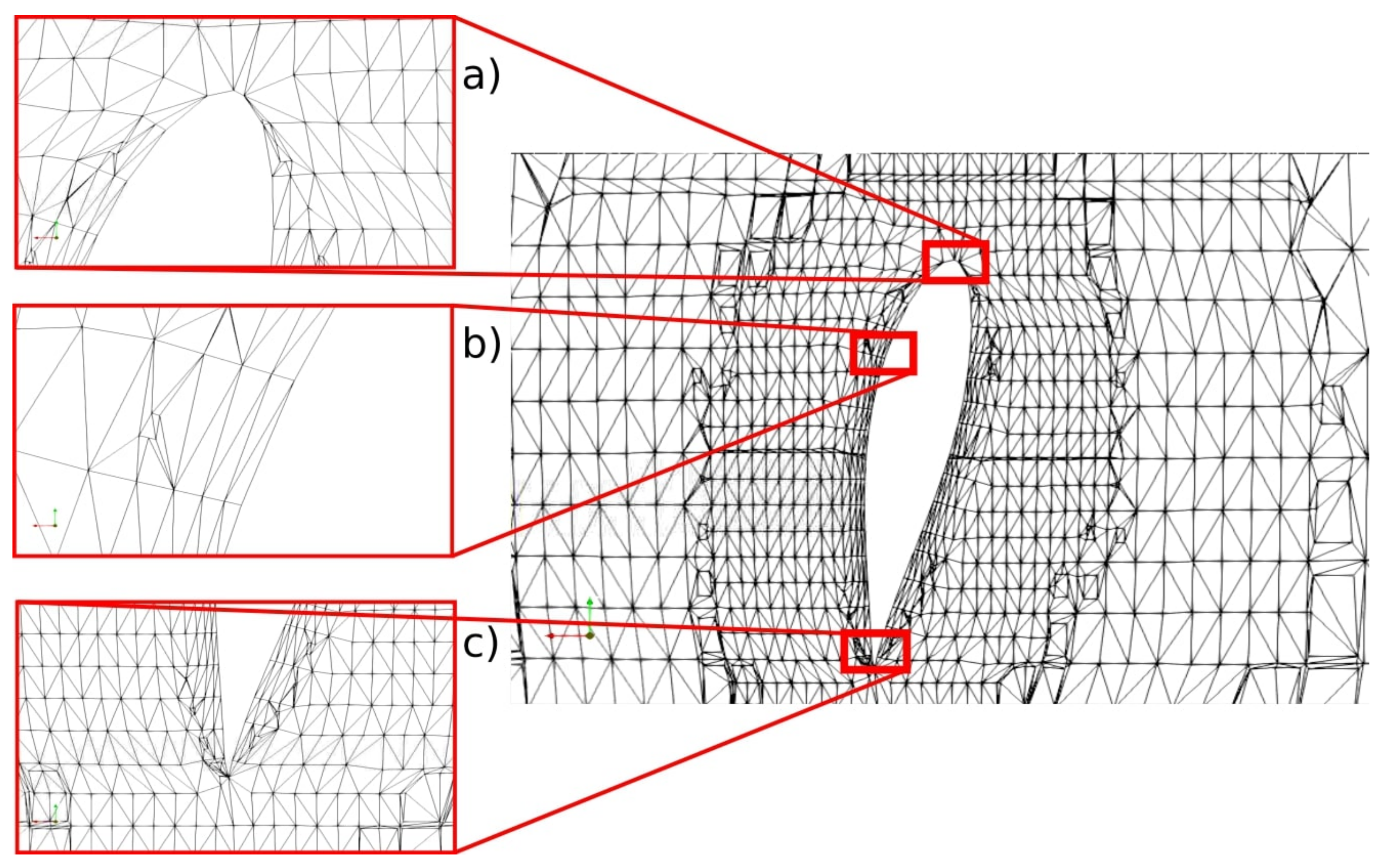
Blade section for a level 5 refinement—the coarsest mesh (#2.1) with a close-up on leading edge (a), trailing edge (c) and upper surface (b). Distorted elements are due to the visualization section.
Figure 9.
Blade section for a level 5 refinement—the coarsest mesh (#2.1) with a close-up on leading edge (a), trailing edge (c) and upper surface (b). Distorted elements are due to the visualization section.

Figure 10.
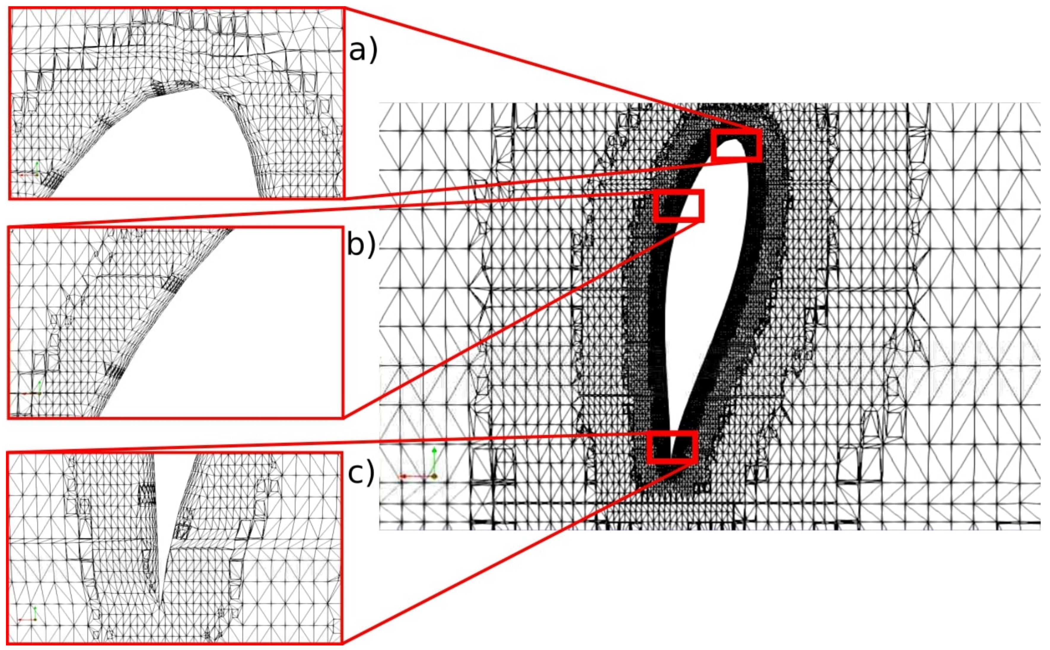
Blade section for a level 9 refinement—the finest mesh (#2.4) with a close-up on leading edge (a), trailing edge (c) and upper surface (b). Distorted elements are due to the visualization section.
Figure 10.
Blade section for a level 9 refinement—the finest mesh (#2.4) with a close-up on leading edge (a), trailing edge (c) and upper surface (b). Distorted elements are due to the visualization section.

Figure 11.
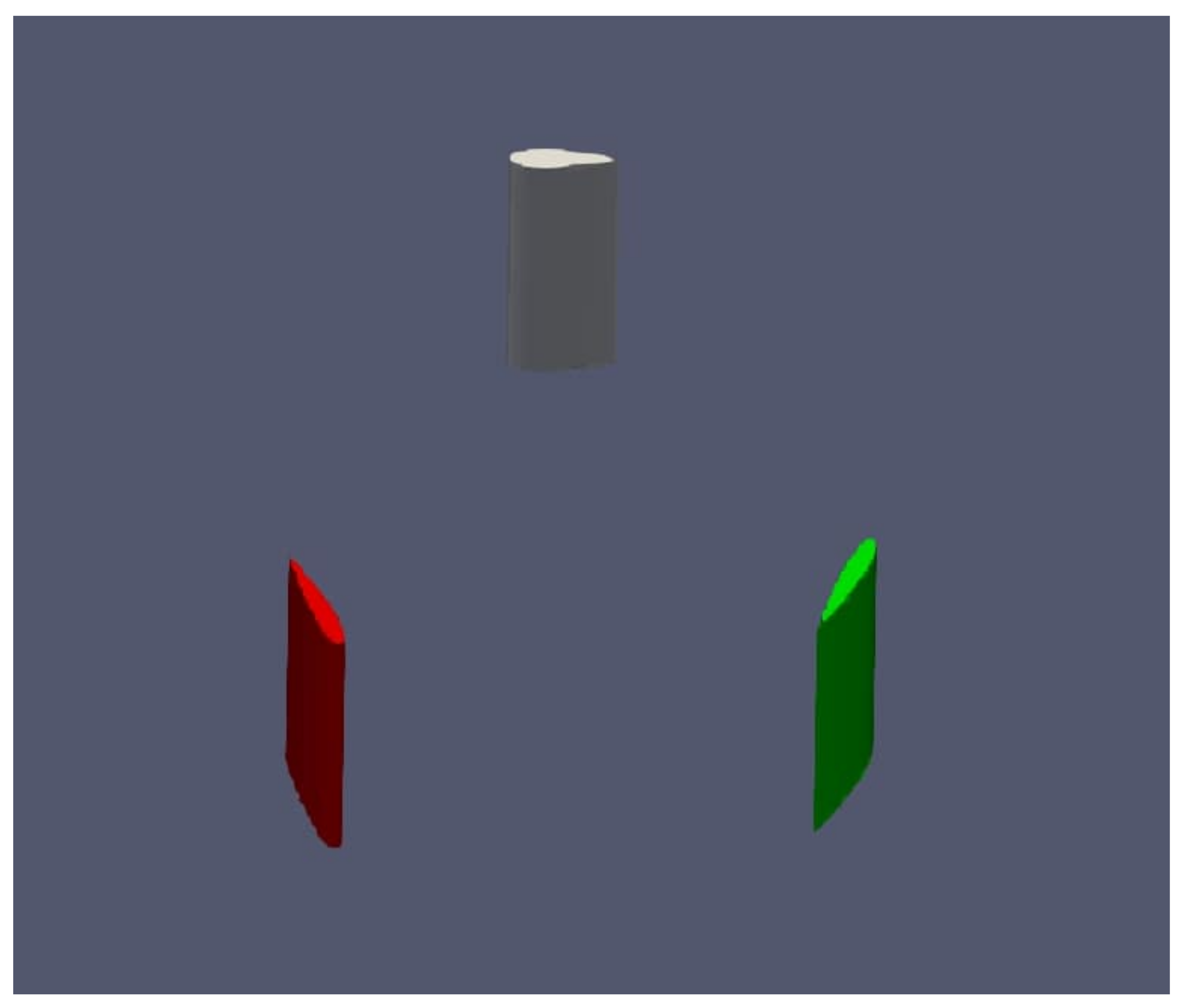
Three-dimensional geometry of the blades of the vertical axis tidal turbine without hub for a sideways view.
Figure 11.
Three-dimensional geometry of the blades of the vertical axis tidal turbine without hub for a sideways view.

Figure 12.
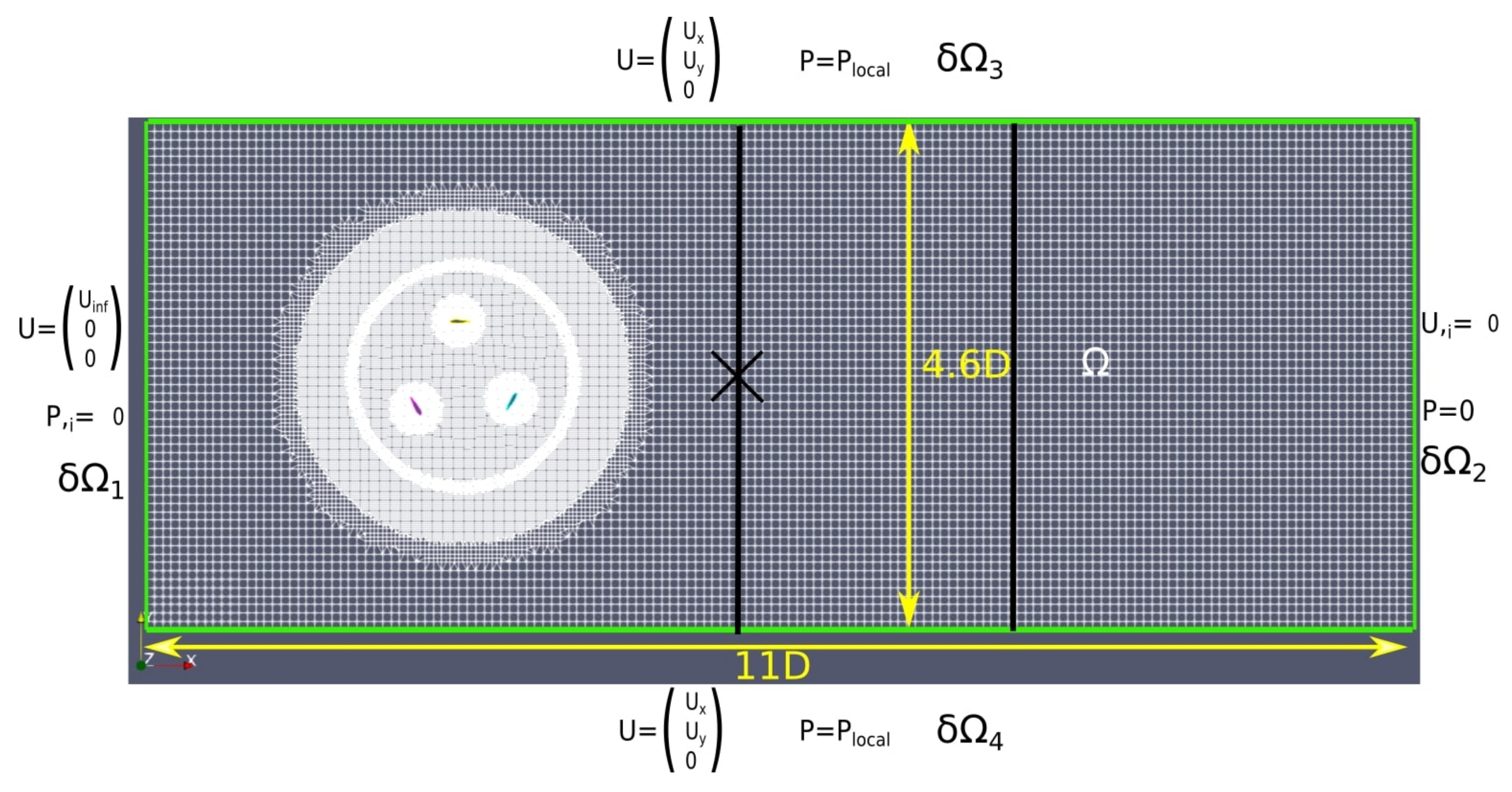
View of X–Y plane for the computational domain with boundary conditions (in green). D is the rotor’s diameter in . U is the flow velocity in , and P is the pressure in . The two black lines (2D and 4D) and the black cross are the extraction lines and the probe, respectively, used in the model validation in Section 3.2.
Figure 12.
View of X–Y plane for the computational domain with boundary conditions (in green). D is the rotor’s diameter in . U is the flow velocity in , and P is the pressure in . The two black lines (2D and 4D) and the black cross are the extraction lines and the probe, respectively, used in the model validation in Section 3.2.

Figure 13.
magnitude along for #1, #2.0, #2.4 and #3 at = 1.2.

Figure 14.
Same legend as previous one but for = 2.

Figure 15.
Time evolution of the vorticity magnitude close to the rotor, inside the AMI zone ( = 2), for coarse (#1 with red line) and refined (#2 with blue line) meshes.
Figure 15.
Time evolution of the vorticity magnitude close to the rotor, inside the AMI zone ( = 2), for coarse (#1 with red line) and refined (#2 with blue line) meshes.

Figure 16.
Time evolution of the power coefficient (Cp) with coarse (red line) and fine (blue line) mesh refinement in the wake.
Figure 16.
Time evolution of the power coefficient (Cp) with coarse (red line) and fine (blue line) mesh refinement in the wake.

Figure 17.
Time evolution of Cp for the cases with (#3 red line) and without a hub (#2.0 blue line).
Figure 17.
Time evolution of Cp for the cases with (#3 red line) and without a hub (#2.0 blue line).

Figure 18.
Cp time evolution for cases #2.0 (blue), #2.1 (red), #2.2 (green), #2.3 (pink) and #2.4 (cyan).
Figure 18.
Cp time evolution for cases #2.0 (blue), #2.1 (red), #2.2 (green), #2.3 (pink) and #2.4 (cyan).

Figure 19.
Relative difference between Cp after 1 s of simulation for cases #2.0 (blue lozenge), #2.1 (red dot), #2.2 (green square), #2.3 (pink plus), #2.4 (cyan cross) and #2.4.
Figure 19.
Relative difference between Cp after 1 s of simulation for cases #2.0 (blue lozenge), #2.1 (red dot), #2.2 (green square), #2.3 (pink plus), #2.4 (cyan cross) and #2.4.

Figure 20.
time evolution for the cases with (#3) and without a hub (#2.0).

Figure 21.
time evolution according to the level of refinement for cases #2.0 (blue), #2.1 (red), #2.2 (green), #2.3 (pink) and #2.4 (cyan).
Figure 21.
time evolution according to the level of refinement for cases #2.0 (blue), #2.1 (red), #2.2 (green), #2.3 (pink) and #2.4 (cyan).

Figure 22.
Relative difference in according to the level of refinement for cases #2.0 (blue lozenge), #2.1 (red dot), #2.2 (green square), #2.3 (pink plus), #2.4 (cyan cross) and #2.4.
Figure 22.
Relative difference in according to the level of refinement for cases #2.0 (blue lozenge), #2.1 (red dot), #2.2 (green square), #2.3 (pink plus), #2.4 (cyan cross) and #2.4.

Figure 23.
Non-dimensional velocity profiles according to the non-dimensional position for experimental data (red lozenges) and model (#2.4) as . The mismatch at was due to the missing hub in the numerical case.
Figure 23.
Non-dimensional velocity profiles according to the non-dimensional position for experimental data (red lozenges) and model (#2.4) as . The mismatch at was due to the missing hub in the numerical case.

Figure 24.
Same legend as for previous figure, but profiles were taken at . The mismatch at was due to the missing hub in the numerical case.
Figure 24.
Same legend as for previous figure, but profiles were taken at . The mismatch at was due to the missing hub in the numerical case.

Figure 25.
depending on the position comparison between case #5 (blue line) and experimental data (red lozenges) at .
Figure 25.
depending on the position comparison between case #5 (blue line) and experimental data (red lozenges) at .

Figure 26.
depending on the position comparison between case #5 (blue line) and experimental data (red lozenges) at .
Figure 26.
depending on the position comparison between case #5 (blue line) and experimental data (red lozenges) at .

Figure 27.
Time evolution of the power coefficient Cp for case #5 (blue line with crosses) and experimental data (red line with plus). The black line is the Cp mean value starting at 0.5 s.
Figure 27.
Time evolution of the power coefficient Cp for case #5 (blue line with crosses) and experimental data (red line with plus). The black line is the Cp mean value starting at 0.5 s.

Figure 28.
Time evolution of the drag coefficient for case #5 (blue line with crosses) and experimental data (red line with plus). The black line is the Cp mean value starting at 0.5 s.
Figure 28.
Time evolution of the drag coefficient for case #5 (blue line with crosses) and experimental data (red line with plus). The black line is the Cp mean value starting at 0.5 s.

Figure 29.
Time evolution of the angular velocity for cases #4.0 (red line), #4.1 (green line) and #4.2 (blue line).
Figure 29.
Time evolution of the angular velocity for cases #4.0 (red line), #4.1 (green line) and #4.2 (blue line).

Figure 30.
Time evolution of the vorticity magnitude at the probe position (, ) after phase shift correction for #4.0 (red line), #4.1 (green line) and #4.2 (blue line).
Figure 30.
Time evolution of the vorticity magnitude at the probe position (, ) after phase shift correction for #4.0 (red line), #4.1 (green line) and #4.2 (blue line).

Figure 31.
Frequency-based spectra of vorticity for the cases #4.0 (red line), #4.1 (green line) and #4.2 (blue line).
Figure 31.
Frequency-based spectra of vorticity for the cases #4.0 (red line), #4.1 (green line) and #4.2 (blue line).

Figure 32.
Time evolution of the angular velocity for forced (blue line, #6.1) and induced (red line, #6.2) rotation.
Figure 32.
Time evolution of the angular velocity for forced (blue line, #6.1) and induced (red line, #6.2) rotation.

Figure 33.
Frequency-based spectra of the vorticity for forced (blue line, #6.1) and induced (red line, #6.2) rotation cases.
Figure 33.
Frequency-based spectra of the vorticity for forced (blue line, #6.1) and induced (red line, #6.2) rotation cases.

Figure 34.
Time evolution of the fluid vorticity at the probe location for forced (blue line, #6.1) and induced (red line, #6.2) rotation.
Figure 34.
Time evolution of the fluid vorticity at the probe location for forced (blue line, #6.1) and induced (red line, #6.2) rotation.


Table 1.
Summary of the characteristic lengths of the cells relative to the levels of refinement.
| Levels | Characteristic Length |
|---|---|
| Level 1 | |
| Level 2 | |
| Level 3 | |
| Level 4 | |
| Level 5 | |
| Level 6 | |
| Level 7 | |
| Level 8 | |
| Level 9 |
Table 2.
Summary of test cases for the horizontal axis turbine according to the level of refinement on the blades and in the wake, the presence or absence of a hub, and the total number of points in the mesh (Nb).
Table 2.
Summary of test cases for the horizontal axis turbine according to the level of refinement on the blades and in the wake, the presence or absence of a hub, and the total number of points in the mesh (Nb).
| Mesh | Level on Blades | Level in Wake | Hub | Nb () |
|---|---|---|---|---|
| Reference case (#1) | Level 6 | Level 1 | No | 1 |
| Wake case (#2.0) | Level 6 | Level 3 | No | 1.9 |
| Blade 5 (#2.1) | Level 5 | Level 3 | No | 1.6 |
| Blade 7 (#2.2) | Level 7 | Level 3 | No | 3.5 |
| Blade 8 (#2.3) | Level 8 | Level 3 | No | 9 |
| Blade 9 (#2.4) | Level 9 | Level 3 | No | 12 |
| Hub case (#3) | Level 6 | Level 3 | Yes | 2.2 |
| Flow-induced L6 (#4.0) | Level 6 | Level 3 | No | 1.9 |
| Forced free rotation speed L6 (#4.1) | Level 6 | Level 3 | No | 1.9 |
| Flow-induced L7 (#4.2) | Level 7 | Level 3 | No | 3.5 |
Table 3.
Summary of test cases for vertical axis turbine according to the level of refinement on the blades and in the wake, the presence or absence of a hub, and the total number of points in the mesh (Nb).
Table 3.
Summary of test cases for vertical axis turbine according to the level of refinement on the blades and in the wake, the presence or absence of a hub, and the total number of points in the mesh (Nb).
| Mesh | Level on Blades | Level in Wake | Hub | Nb () |
|---|---|---|---|---|
| Forced for validation (#5) | Level 6 | Level 3 | No | 1.2 |
| Forced free speed (#6.1) | Level 6 | Level 3 | No | 1.2 |
| Flow induced (#6.2) | Level 6 | Level 3 | No | 1.2 |
Table 4.
Table of the physical parameters used in simulations for horizontal and vertical axis cases.
Table 4.
Table of the physical parameters used in simulations for horizontal and vertical axis cases.
| Parameter | Horizontal Axis Turbine | Vertical Axis Turbine | Unit |
|---|---|---|---|
| 1025 | 998 | ||
| 4 | 2 | - |
Table 5.
Summary of the Cp values after 1 s of simulation depending on the level of refinement on the blades. The relative difference compared to the level 9 simulation is given in the last column.
Table 5.
Summary of the Cp values after 1 s of simulation depending on the level of refinement on the blades. The relative difference compared to the level 9 simulation is given in the last column.
| Level | Case | Cp | Relative Difference |
|---|---|---|---|
| 5 | #2.1 | 0.2688 | |
| 6 | #2.0 | 0.1341 | |
| 7 | #2.2 | 0.0787 | |
| 8 | #2.3 | 0.0095 | |
| 9 | #2.4 | 0 |
Table 6.
Summary of the Cd values after 1 s of simulation depending on the level of refinement on the blades. The relative difference compared to the level 9 simulation is given in the last column.
Table 6.
Summary of the Cd values after 1 s of simulation depending on the level of refinement on the blades. The relative difference compared to the level 9 simulation is given in the last column.
| Level | Case | Cd | Relative Difference |
|---|---|---|---|
| 5 | #2.1 | 0.5698 | 0.0501 |
| 6 | #2.0 | 0.6120 | 0.0.0203 |
| 7 | #2.2 | 0.0025 | |
| 8 | #2.3 | 0.0020 | |
| 9 | #2.4 | 0 |
Table 7.
Coefficient values with their relative differences with the experiment data.
| Coefficient | Value | Relative Difference |
|---|---|---|
| 0.3729 | 0.070 | |
| 0.3887 | 0.031 | |
| 0.5998 | 0.1552 | |
| 0.6418 | 0.09 |
Table 8.
Coefficient values with their relative differences with the experiment data.
| Coefficient | Experimental | Numerical | Relative Difference |
|---|---|---|---|
| 0.24 | 0.2779 | 0.1576 | |
| 1.13 | 1.3806 | 0.1800 |
Publisher’s Note: MDPI stays neutral with regard to jurisdictional claims in published maps and institutional affiliations. |
© 2021 by the authors. Licensee MDPI, Basel, Switzerland. This article is an open access article distributed under the terms and conditions of the Creative Commons Attribution (CC BY) license (http://creativecommons.org/licenses/by/4.0/).
Share and Cite
MDPI and ACS Style
Robin, I.; Bennis, A.-C.; Dauvin, J.-C. 3D Simulation with Flow-Induced Rotation for Non-Deformable Tidal Turbines. J. Mar. Sci. Eng. 2021, 9, 250. https://doi.org/10.3390/jmse9030250
AMA Style
Robin I, Bennis A-C, Dauvin J-C. 3D Simulation with Flow-Induced Rotation for Non-Deformable Tidal Turbines. Journal of Marine Science and Engineering. 2021; 9(3):250. https://doi.org/10.3390/jmse9030250
Chicago/Turabian StyleRobin, Ilan, Anne-Claire Bennis, and Jean-Claude Dauvin. 2021. "3D Simulation with Flow-Induced Rotation for Non-Deformable Tidal Turbines" Journal of Marine Science and Engineering 9, no. 3: 250. https://doi.org/10.3390/jmse9030250
Note that from the first issue of 2016, this journal uses article numbers instead of page numbers. See further details here.