
Generating Synthetic Sidescan Sonar Snippets Using Transfer-Learning in Generative Adversarial Networks


1
German Aerospace Center, Institute for the Protection of Maritime Infrastructures, Fischkai 1, D-27572 Bremerhaven, Germany
2
Institute of Water-Acoustics, Sonar-Engineering and Signal-Theory, City University of Applied Sciences Bremen, Neustadtswall 30, D-28199 Bremen, Germany
3
Institute of Technologies and Management of the Digital Transformation, University of Wuppertal, Rainer-Gruenter-Straße 21, D-42119 Wuppertal, Germany
*
Author to whom correspondence should be addressed.
J. Mar. Sci. Eng. 2021, 9(3), 239; https://doi.org/10.3390/jmse9030239
Submission received: 8 January 2021
/
Revised: 9 February 2021
/
Accepted: 15 February 2021
/
Published: 24 February 2021
(This article belongs to the Special Issue Underwater Computer Vision and Image Processing)
Abstract
:The training of a deep learning model requires a large amount of data. In case of sidescan sonar images, the number of snippets from objects of interest is limited. Generative adversarial networks (GAN) have shown to be able to generate photo-realistic images. Hence, we use a GAN to augment a baseline sidescan image dataset with synthetic snippets. Although the training of a GAN with few data samples is likely to cause mode collapse, a combination of pre-training using simple simulated images and fine-tuning with real data reduces this problem. However, for sonar data, we show that this approach of transfer-learning a GAN is sensitive to the pre-training step, meaning that the vanishing of the gradients of the GAN’s discriminator becomes a critical problem. Here, we demonstrate how to overcome this problem, and thus how to apply transfer-learning to GANs for generating synthetic sidescan snippets in a more robust way. Additionally, in order to further investigate the GAN’s ability to augment a sidescan image dataset, the generated images are analyzed in the image and the frequency domain. The work helps other researchers in the field of sonar image processing to augment their dataset with additional synthetic samples.
1. Introduction
Collecting a dataset of sidescan sonar images from objects underwater is a cumbersome task since the location of the objects is, on principle, not known in advance. As an alternative, manually placing objects on the seafloor and capturing images with a sidescan sonar mounted on an autonomous underwater vehicle (AUV) is very time- and cost-intensive, especially if a high variability in the dataset is desired. Thus, simulating sonar data has been part of research efforts for several years [1,2,3]. The simulated data can be used to enrich the real dataset in order to improve the automatic analysis of sonar images, e.g., by having a larger dataset for the training of a deep-learning-based classifier. In recent years, generative adversarial networks (GAN) [4] have become a successful algorithm for generating synthetic images. Their field of application ranges from face-generation [5,6] to image translation tasks [7]. Much research work regarding GANs has been done in designing architectures and training methods which leverage the quality of the generated images, as in StyleGAN2 [6], which uses a special style-based generator to produce high-resolution images. A comprehensive review of state-of-the-art GANs for various image processing tasks can be found in [8].
Recently, GANs have been applied to the field of underwater acoustic imaging [9,10,11,12]. By generating synthetic high-quality sonar images, the necessity of a large database of real images may be reduced. However, the training process of a GAN also requires training data, and a small training dataset may increase the probability of the occurrence of mode collapse [13]. In the case of mode collapse, the GAN generator produces the same image regardless of the input noise, and is not able to recover from this. Several approaches have been developed in recent years to improve the training of a GAN when only few data are available [14,15,16,17,18,19]. In [19], the so-called stochastic discriminator augmentation is used to artificially increase the amount of training data and prevent the generator from learning these augmentations. However, thousands of images are still required to train a high-resolution GAN like StyleGAN2. In addition to data augmentation, the current research focuses on transfer-learning methods for GANs in cases with few data samples [14,15,16,17]. During the transfer-learning in [16,17] the first layers of the discriminator, the discriminator and generator, are kept fixed. Zhao et al. propose an adaptive filter modulation to further adapt the weights in the fixed layers of the discriminator and generator [17]. Both methods show good results when applied to natural images, even if fewer than 1.000 images are used for transfer-learning. However, these approaches are based on transferring knowledge from a large dataset of natural RGB images to other natural RGB images. Since the characteristics of sidescan sonar images are fundamentally different from those natural images, most features learned in the pre-training, such as ones based on color or specific shapes, are useless.
In most approaches that use GANs for generating sonar images, the GANs are trained to learn an image-translation from low-complexity ray-traced images to real sonar images [9,10]. These approaches use hundreds of real sonar images from an object, which seems few compared to other large deep-learning datasets. However, several sea trials are required to capture this amount of real sonar data. Having fewer real sonar images can be a critical factor in the image-translation, since many ray-traced images would be mapped to only a few real samples. In [12], ray-traced snippets of tires are used in a pre-training phase of a GAN so that it can learn to generate the geometric properties. Afterwards, a subsequent fine-tuning step is used to make this GAN generate realistic sidescan sonar snippets. This procedure of transfer-learning has been shown to decrease the occurrence of mode collapse.
We expand our previous work [12] and show that while the problem of mode collapse is reduced, the pre-training makes the GAN very sensitive to the input distribution. On the training dataset for the fine-tuning step, the gradient of the discriminator of the GAN vanishes, i.e., the gradient, becomes zero, leaving the GAN unable to learn. Several experiments are conducted to find the best way to prevent the discriminator’s gradient from vanishing. The result is a robustification of the transfer-learning process of a GAN. Afterwards, additional analyses of the generated images are carried out to investigate the quality and variability of the generated data as well as the quality in the frequency domain.
In summary, the main contributions of this paper are:
- An in-depth analysis of the generation of sidescan sonar image snippets using transfer-learning in GANs;
- A solution to the problem of the vanishing gradient when fine-tuning the discriminator;
- An analysis of the generated sidescan sonar snippets which shows that this transfer-learned GAN can slightly improve the classification accuracy of a convolutional neural network (CNN) on an unbalanced dataset.
The remainder of this paper is structured as follows: Section 2 describes the real and simulated data used in this work. Furthermore, the GAN used for generating the synthetic sonar snippets and the procedure of transfer-learning this GAN is explained. In Section 3, the vanishing of the discriminator’s gradient and ways to deal with this problem are analyzed. Later in this section, the generated images are used to augment a dataset for classification purposes. Additionally, by clustering the generated images, the variability in the images is analyzed. Finally, in Section 4, the main findings of this work are summarized and discussed.
2. Materials and Methods
2.1. Real Sidescan Sonar Image Data
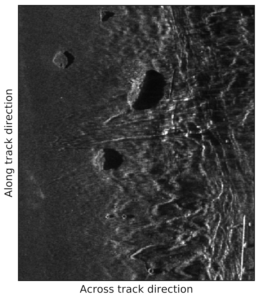
Over the course of several sea and harbor expeditions, sidescan sonar data were collected with an Edgetech 2205 sidescan sonar mounted on a SeaCat AUV (ATLAS ELEKTRONIK GmbH, Bremen, Germany). The sidescan sonar operates at a center frequency of 850 kHz, with a bandwidth of 45 kHz. An experimental signal-processing chain produces gray-scaled images in a waterfall manner, i.e., the individual signals of each ping period are consecutively stacked on top of each other. These waterfall images have a pixel resolution of 10 cm in along and across the track direction. Figure 1 shows an example of a processed waterfall image.
Several different object classes were manually labeled in these sidescan images. This work focuses on the objects of class Tire, due to their well-defined geometric properties, which are required when modeling the object in the ray-tracer. Since some trials were carried out in the same area, multiple snippets from the same object exist. The snippets are split nearly 50/50 between training and test sets, with snippets from the same tire being either all in the training or all in the test set. In Table 1, an example of the snippets and the number of samples in the training and test dataset are listed. As one can see, the number of samples of the class Tire is very limited. However, Steiniger et al. showed that, using transfer-learning, a GAN can be trained with such a small dataset [12].
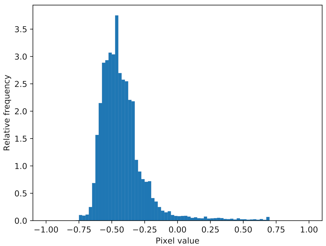
All pixels in the waterfall images are clipped to the interval , in order to increase the contrast in the image. Prior to extracting the object snippets, the pixel values are linearly mapped to the interval . The extracted snippets are rescaled to pixels using bicubic interpolation. Images from the port-side sonar are flipped such that the shadow of an object always lies on the right side of the object. During training, the dataset is augmented using horizontal flipping, since vertical flipping would cause the shadow to lie on the left side of the object again. The histogram of the pixel values from all tire snippets after the aforementioned processing steps is shown in Figure 2.
2.2. Ray-Traced Sonar Snippets
For the pre-training step of the TransfGAN, explained in Section 2.3, ray-traced images from tires are used. Similar to [10,12], the ray-tracer Povray is used to generate synthetic sidescan sonar snippets. Those images can be calculated quickly and in different scenarios, e.g., distance from the AUV to the object. A Python script is used to automatically adapt the Povray simulation, run it and extract the snippet. When extracting the snippet from the whole simulated scene, a small random shift is applied, such that the position of the object in the snippet varies slightly. This reflects the process of manual labeling and extracting real snippets. The parameters vary, and their value-ranges in the simulation are given in Table 2. The resolution is set such that it matches the one from the sonar processing.
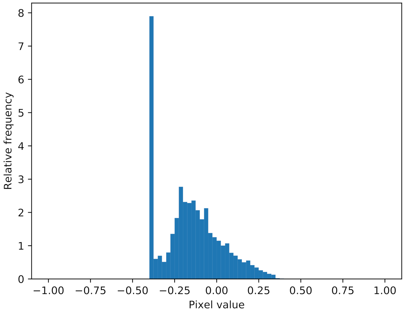
In total 10,000 slightly different snippets were generated. They were split into training and test sets, with a ratio of 2:1. Figure 3 shows three examples of ray-traced tires. When used in the pre-training, the snippets are rescaled to pixels, again using bicubic interpolation. The histogram of the ray-traced images is displayed in Figure 4. Compared to the real sidescan snippets, a characteristic of the simulation becomes visible, which is that no structure is applied to the object or the background. One the one hand, this makes the ray-tracing step as simple as possible but on the other hand, it means that each simulated image mainly consists of three different pixel values, which does not reflect a common distribution in sonar images. The strong peak in the histogram at −0.4 arises from the fact that the intensity of the highlight and background varies with the distance from the AUV to the object but the intensity of the shadow stays the same.Since the histogram is calculated from all simulated snippets, the variation in highlight and background intensity is averaged out. Furthermore, a shift between the two histograms can be observed, indicating a brighter background in the ray-traced snippets. Thus, the main purpose of the ray-traced snippets is to give the GAN information about the geometric shape of the highlight and shadow regions in the image. Adapting the pixel distribution in the ray-traced snippets to better match the real data is a task for future work.
2.3. Training a GAN with Transfer-Learning
A GAN is a combination of a generator and a discriminator network which are trained alternately so that the generator learns to map a noise distribution onto a distribution given by the input data. The discriminator’s task is to reject samples created by the generator, forcing the generator to produce better images, which are more difficult to distinguish from the real data. A common problem when training a GAN is the so-called mode collapse [20], where the generator produces the same image regardless of the input noise. Transfer-learning has shown to improve the training of a GAN and to reduce the occurrence of mode collapse [12,17]. The TransfGAN described in [12] is in a first pre-training step trained with ray-traced images, which should help the generator to learn the geometric shape of the object. In a second step, the pre-trained GAN is fine-tuned with the real sidescan snippets. Figure 5 shows the individual training steps of the TransfGAN.
For the structure of the generator and discriminator network, the ones from [12], where an auxiliary classifier GAN (ACGAN) [21] is used, are adapted. An ACGAN uses the class of an object as an additional input to the generator, and as an additional output to be predicted by the discriminator. This has been shown to increase the quality of the generated images and is a way to condition the GAN to generate images for a given class. However, in this work, only one class is considered, which makes the auxiliary loss introduced by the ACGAN needless. Thus, our networks have no conditional class input and the discriminator has only one fully connected output layer to predict if the sample it receives is real or fake. The configurations of both networks are shown in Table 3 and Table 4, respectively. The generator network G takes a latent vector as an input and generates a synthetic image . Transposed convolutional layers are used to upsample the latent vector to the required image size of pixels. The input to the discriminator network D is either a real image or a generated one. For each image, this network outputs a probability that the image is real, i.e., for a perfect discriminator and .
The TransfGAN is pre-trained for 500 epochs with a batch size of 100 using the Adam optimizer [22], with a learning rate of 0.0002 and an exponential decay rate for the 1st moment estimates of 0.5. Both networks are trained alternately, where the discriminator is set to minimize
and the generator to minimize
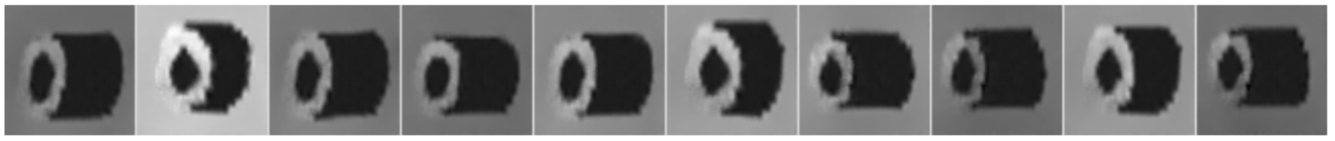
The latent vector contains 100 samples of a uniform distribution. Some generated samples from the pre-trained TransfGAN are shown in Figure 6.
After pre-training, the TransfGAN is fine-tuned with the real sidescan data. The fine-tuning takes place for 200 Epochs and a batch size of 36, so one iteration covers all real and augmented tire snippets. The learning rates for the generator and discriminator are selected using a grid search over the values , while the exponential decay rate for the 1st momentum estimates is kept at 0.5.
3. Results
3.1. Analysis of the Vanishing Gradient
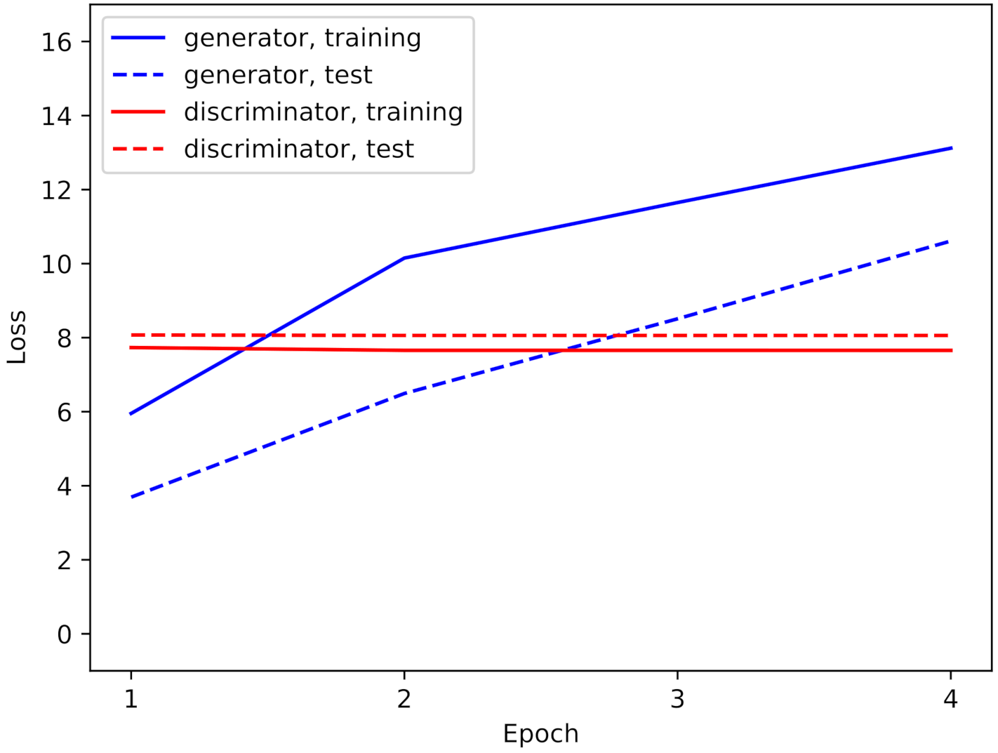
During the fine-tuning step of the TransfGAN, the loss behaves as shown in Figure 7. The loss of the discriminator remains constant while the loss of the generator increases.
Looking at the training process of a neural network, the weights are updated using the gradient of a loss function with respect to the individual weights. In the very basic stochastic gradient descent, the update follows the rule
where are the weights from the i-th iteration, is the learning rate, l is the loss function and all calculations are taken element-wise. Using the Adam optimizer [22] the update rule modifies to
where
and
where are hyperparameters. Here, the gradient of the loss function with respect to the weights is used again. The exponential moving averages of the gradient m and the squared gradient v are initialized with a value of zero. Consequently, if this gradient is zero, no update to the weights is made. Figure 8 shows the gradients of the discriminator over the first four epochs for the real sidescan snippet (red) and the fake images generated by the TransfGAN’s generator (blue). It becomes clear that the gradient of the TransfGAN’s discriminator vanishes when it is trained with the real sidescan snippets. Due to the chain rule of calculus used in the back-propagation algorithm for training a neural network, a vanishing gradient in the last layer of the network leads to a gradient of zero in the remaining ones. Furthermore, the GAN is not able to recover from this vanishing gradient problem and will stay in this stage in all consecutive epochs.
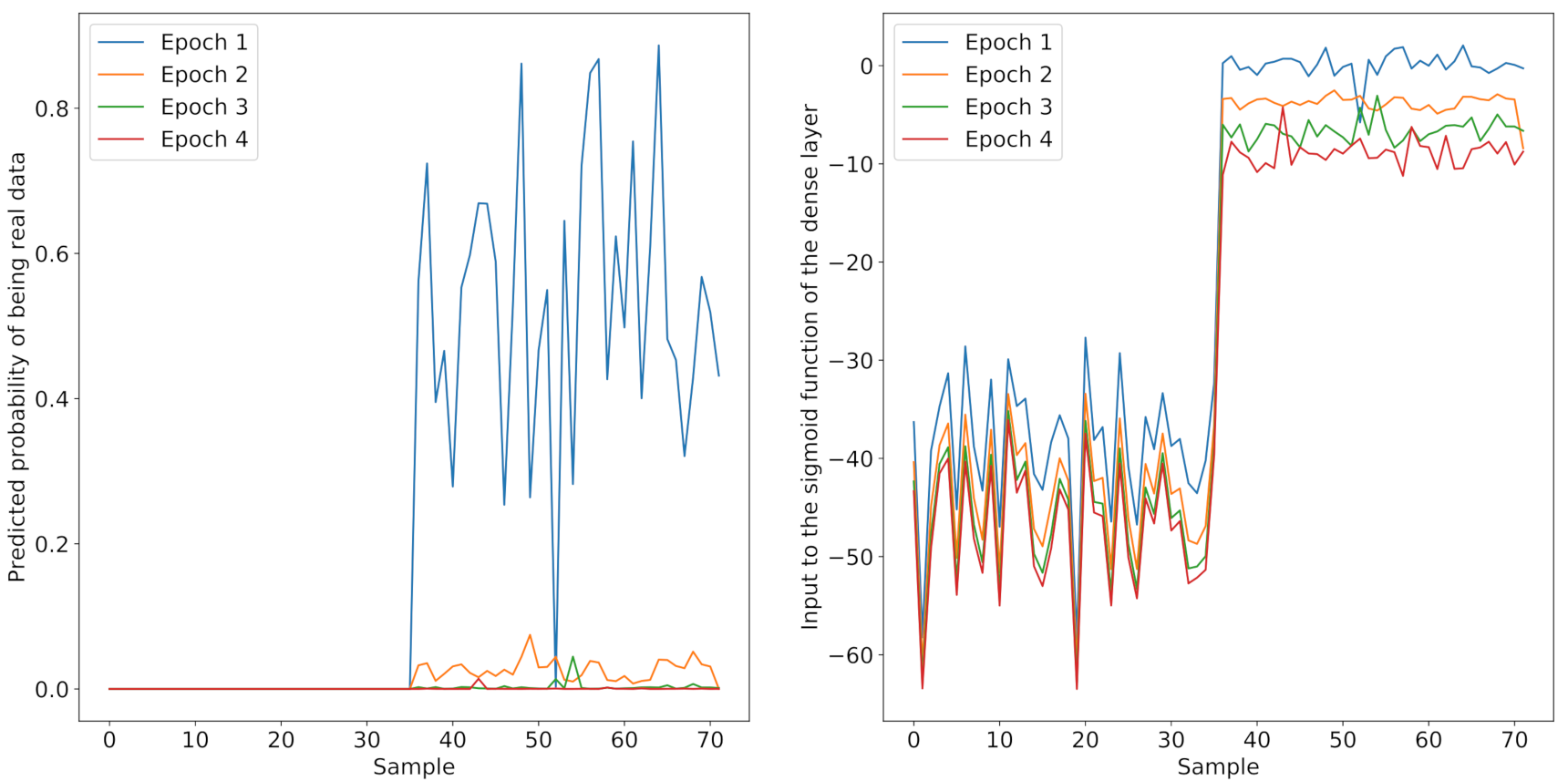
In order to explain the occurrence of the vanishing gradient in the discriminator, Figure 9 displays the predictions of the discriminator before updating the weights for the first four epochs. For the real sidescan snippets (sample 0–35), the discriminator classifies all images as fake. The right sub-figure in Figure 9 shows the output of the dense layer prior to processing by the sigmoid function. For the real samples, the sigmoid function saturates. Note that a sigmoid(−40) is already . This reveals a fundamental problem in the transfer-learning of the GAN. During the pre-training, the discriminator sees ray-traced images as real images. These ray-traced images often consist of only a few pixel values, as shown in the histogram in Figure 4. This makes it likely that the discriminator will reject all samples which differ from this pixel-value distribution. In the fine-tuning step, the sidescan sonar snippets become the real images, but due to the pre-training, the discriminator will reject them. This problem remains if, in the pre-training step, a small portion of noise is added to the ray-traced images in order to disturb the pixel value distribution. However, the effect of adjusting the pixel distribution in the highlight, shadow and background regions of the ray-traced snippets according to a more realistic distribution still needs to be investigated. In the following section, experiments are conducted to investigate possible solutions to this vanishing gradient problem.
3.2. Experimental Study
Since the vanishing gradient in the discriminator only becomes visible in the fine-tuning step, this would make it necessary to re-initialize the GAN and to repeat the pre-training. A more convenient way of doing this would be to make the fine-tuning step more robust, so that it can deal with the vanishing gradient. Two slightly different approaches are analyzed in this study. In Experiment “All”, the weights of all layers in the discriminator are re-initialized prior to the fine-tuning step. Only the generator keeps the information from the pre-training step, while the discriminator is trained from scratch. This, however, would delete already learned features of the discriminator, which may still be useful for classifying the sidescan snippet into real or fake, e.g., basic geometric features. Therefore, in the Experiment “Last”, the re-initialization of only the last layer of the discriminator, i.e., the fully connected layer, will be analyzed. Here, the features learned by the convolutional layers in the discriminator (see Table 4) are used in the fine-tuning step.
For both experiments, a grid-search over the learning rate is carried out to determine its optimum value. The learning rate for the generator and for the discriminator is allowed to differ since the (partial) re-initialization of the discriminator may give the generator a head start in the fine-tuning phase. For the same reason, training only the discriminator for a few epochs before fine-tuning the whole GAN is analyzed as well. During the grid search, the learning rates are set to . In all experiments, the TransfGAN is fine-tuned for 200 epochs. This number of epochs is sufficient to see if the applied method is able to train the TransfGAN without vanishing gradient. All experiments are conducted three times to account for the randomness in the re-initialization, resulting in a total of 300 experiment runs. While reporting the results of all these runs is beyond the scope of this article, the main findings are presented.
One outcome from the previous analysis of the vanishing gradient is that the loss of the discriminator stays constant if its gradient vanishes. Thus, a decaying loss indicates a success in countering the vanishing gradient. However, this criterion alone does not allow for direct statements about the quality of the generated images. A qualitative analysis of the images generated by the TransfGAN after fine-tuning will be carried out to rate the success of the two approaches “All” and “Last”. The criteria for sufficient quality of the generated images are:
- Physically meaningful highlight and shadow;
- Shadow connected to the right side of the object;
- Realistic pixel value distribution in highlight, shadow and background regions;
- No mode collapse.
As expected in most cases, both re-initialization approaches solve the problem of the vanishing gradient. Only for a discriminator learning rate of does the problem remain. Since a gradient of zero means no update in the discriminator, the extra training also does not help in these learning rate configurations. The learning rate is too high for the discriminator to converge to a minimum.
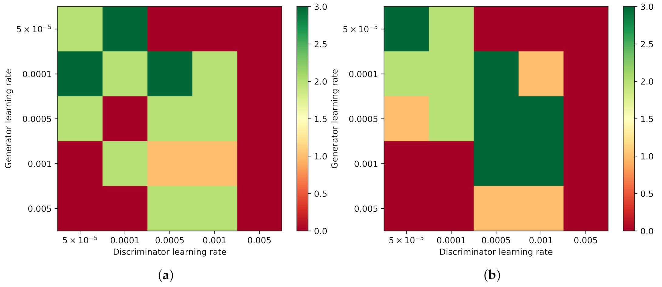
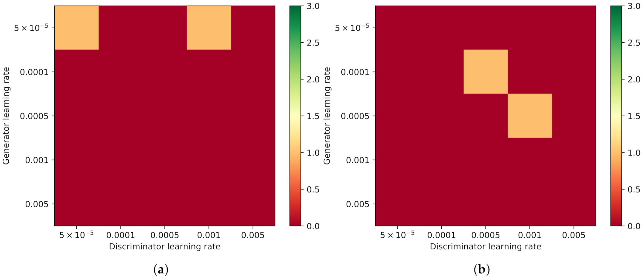
For all configurations of the experiments, the quality of the generated images is rated according to the criteria defined above. If all criteria are satisfied, a value of one is manually assigned to this configuration and a zero otherwise. Figure 10 shows the rating quality of the images for the grid search configurations when re-initializing the last layer (Experiment “Last”). Because the training is done three times per experiment, the quality rating can be averaged over these three runs. A dark green value indicates that, in all three runs, the quality was good according to the criteria, and the light green indicates that only two of the three trained TransfGANs produce good images. The orange field encodes one TransfGAN which produces good images, and the red one indicates that all images lack one or all quality characteristics.
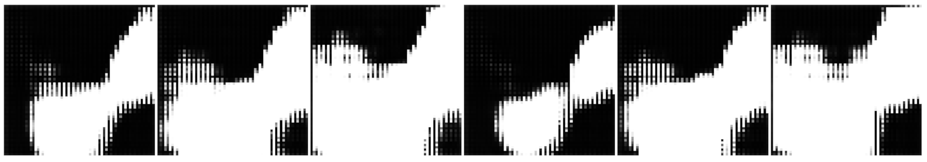
In Experiment “Last”, the images for lack quality because they are not showing a realistic pixel distribution due to the remaining presence of the vanishing gradient. For low generator learning rates () and higher discriminator learning rates, the generator is not able to generate good images and a noisy pattern is visible. Examples of bad-quality images are given in Figure 11. This pattern remains visible if the TransfGAN is trained for an additional 300 epochs.
If the generator learning rate is large (), it can move into some regions in the loss-space where no highlight and shadow are generated. An example for this failure is shown in Figure 12. This type of error occurs with and without the extra training of the discriminator and for all discriminator learning rates.
When all layers of the discriminator are re-initialized (Experiment “All”), the TransfGAN is not able to learn to generate realistic sidescan snippets, as can be seen in Figure 13. Since, in this experiment, only the generator is able to benefit from the pre-training, the results indicate that the number of training samples is not enough to train the whole discriminator from scratch.
Besides the noisy pattern or cases in which no object at all is generated, another error arising using this approach is that the images look blurry. Figure 14 shows some examples of this type of error, which occurs mostly for larger in combination with smaller . In addition, the presence of mode collapse can be observed in these examples, since all images look the same but were generated by a different noise vector. Mode collapse happened in multiple runs in different learning rate combinations in Experiment “All”, but not in Experiment “Last”, where only the last layer of the discriminator was re-initialized. This again indicates that it is essential to keep information from the pre-training in the discriminator during fine-tuning when the number of training samples is limited.
3.3. Generated Image Analysis
In order to analyze the quality of the generated images from the TransfGAN, of which only the last layer was re-initialized, three additional experiments are carried out. First, besides the qualitative analysis from the previous section, the ability of the generated images to serve as an augmentation dataset for a deep learning classifier is analyzed. In addition, the diversity in the generated samples is investigated. Finally, an analysis of the frequency domain of the images is carried out.
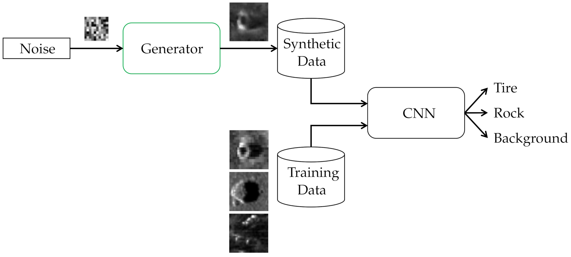
For the first experiment, a CNN is used to classify sidescan sonar snippets into the classes Tire, Rock and Background. The number of samples in each class is given in Table 5, where an imbalance between the number of samples of class Tire and Rock or Background can be seen. The structure of the CNN is taken from [12] and shown in Table 6.
This CNN is trained once with the training set specified in Table 5, and once with an additional 18 tire samples generated by a TransfGAN. Figure 15 illustrates this augmentation scheme.
Following the results from the previous experiment, re-initialization of the last layer of the discriminator was applied to the TransfGAN. Three different configurations of the TransfGAN, which have been shown to generate good images, are compared:
- , , no extra training of the discriminator prior to the fine-tuning
- , , no extra training of the discriminator prior to the fine-tuning
- , , with extra training of the discriminator prior to the fine-tuning
The balanced accuracy
and the macro F1 score
with are used as performance measures. The classification experiments were carried out ten times to account for the random initialization of the CNN. Table 7 reports the mean and standard deviation of the two metrics over these ten runs.
The results show a slight improvement in balanced accuracy and in the macro F1 score of 1% when the training dataset is augmented with generated snippets. Only a negligible difference is seen between the performance achieved from using different TransfGANs. Compared to the results from [12], the performance of the baseline CNN without synthetic augmentation is worse, which can be explained by differences in the sonar data themselves. The increase in classification performance due to the synthetic augmentation is not as large either. Since the variability of the data used for augmentation is a critical factor for potential performance increase, the ability of the TransfGANs used in the classification experiment to generate different images is further investigated.
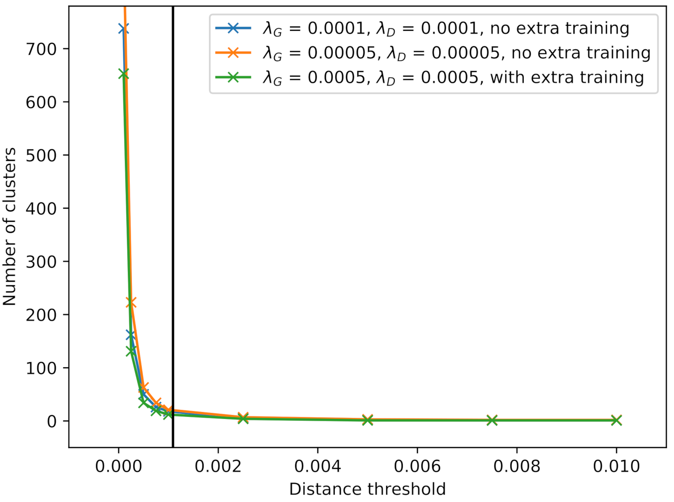
To measure the variability in the generated images, 1000 snippets are generated and clustered by use of the pixel-wise Euclidean distance
between two images and , where, for the generated snippets, . This distance measure is sensitive to translation, i.e., if the same tire was generated by the TransfGAN but placed at different locations inside the snippet, the distance would be large. Since translation can be seen as a type of additional augmentation, it should not harm the variability measure. The pixel-wise Euclidean distance is calculated between all pairs of the 1000 images. Starting with the first image, all other images with a distance smaller than a certain threshold form a cluster to this image. The next not-already-clustered image is then taken as the starting point for the next cluster. Finally, the number of clusters can be seen as the number of different images generated by the TransfGAN, or, in other words, as a measure for image variability. All three TransfGANs from the classification experiment are analyzed in this way. Figure 16 displays the number of clusters for different thresholds. The black line indicates the mean distance between all images as a reference. If the distance threshold for calculating the clusters is set too high, it can be observed that the resulting images, which serve as the center of each cluster, still look very similar. From this observation, the threshold can be set to 0.001 in order to give a reasonable number of different images. For this threshold, the number of clusters is 12, 18 and 21, respectively. When generating the 18 snippets for the augmentation dataset, the probability of generating a very similar image multiple times is high, which may explain the only slight increase in classification performance.
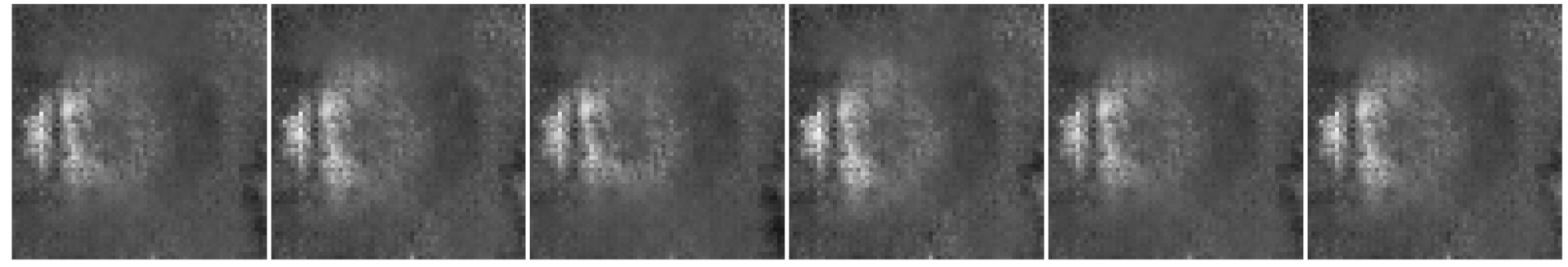
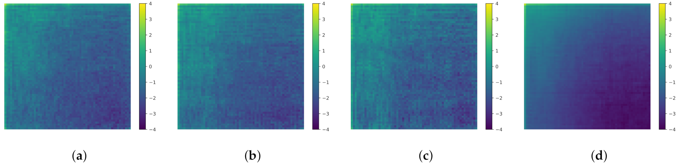
Finally, the generated images are analyzed in the frequency domain. The work of [23] has shown that images generated by a GAN often contain artifacts in the frequency domain which make these images easy to detect as fake when they are processed in the frequency domain. The images from the previous experiment are transformed using the 2D discrete cosine transformation, as is done in [23]. The mean spectra over the 1000 images for the three TransfGANs are displayed in Figure 17 together with the mean spectrum for the real tire images. The upper left corner of the images indicates the low-frequency components and the lower right corner the high-frequency components, respectively. The spectra are displayed in a logarithmic scaling.
All three spectra of the generated images look more noisy compared to the one of the real sidescan snippets, but do not show the artifacts described in [23]. The authors of [23] argue that the artifacts arise due to the upsampling methods used in the generator of the GANs which they have studied. They focus on GANs which were trained on the celebA and LSUN bedrooms datasets, containing images with more details compared to sidescan snippets. Moreover, the resolution of the images is larger than the one of the sidescan snippets with , which results in one fewer upsampling operation. Consequently, the effect from the upsampling on the spectra is smaller.
4. Discussion and Conclusions
This work has contributed to the field of generating synthetic sidescan sonar data by giving an in-depth analysis of a transfer-learning procedure to train a GAN with limited sonar data. The vanishing of the gradient of the discriminator has been shown to be a general problem when applying transfer-learning to GANs, since, in the pre-training, the discriminator may converge into a region where it will reject real samples in the fine-tuning step. This may not be as critical for applications other than imaging sonar, where more complex data can already be used in the pre-training step. However, with the idea in mind that the data in the pre-training should be simple in order to quickly create this data and to learn simple features in this step, finding a way to deal with the vanishing of the discriminator’s gradient becomes necessary. Our presented solution of re-initializing the discriminators last layer prior to the fine-tuning step has shown to make the training of the TransfGAN more robust. No vanishing gradient or mode collapse is present in this case. However, the increase in the performance of a classifier CNN when augmented with synthetic data from this GAN is small. Due to the re-initialization, some information from the pre-training is lost. Furthermore, the training set is very small, leading to a low variability in the images generated by the TransfGAN. A larger dataset may improve the generation capability of the TransfGAN, and thus the performance of a classifier even further. In addition, some information about the pixel-value distribution in sonar images can also be drawn from background images in which no object is present. Such snippets can easily be extracted from a sidescan sonar image. Extracting and feeding this information into the fine-tuning process of the TransfGAN may improve the quality and variability of the generated images. Moreover, adapting the pixel distribution in the highlight, shadow and background regions of the ray-traced images according to a more realistic distribution for sidescan sonar images and its effect on the transfer-learning needs to be investigated. Finally, future work will also focus on additional ways to train a CNN for the classification of a small sidescan sonar image dataset. Transferring knowledge from well-known CNNs like EfficientNet [24], pre-trained on natural images, to the sonar domain, e.g., by training on a gray-scaled version of the Imagenet dataset or other data more similar to sonar images, will be investigated.
Author Contributions
Conceptualization, Y.S., T.M. and D.K.; methodology, Y.S.; software, Y.S.; validation, Y.S., T.M. and D.K.; formal analysis, Y.S. and T.M.; investigation, Y.S. and T.M.; resources, Y.S. and D.K.; data curation, Y.S.; writing—original draft preparation, Y.S.; writing—review and editing, T.M. and D.K.; visualization, Y.S.; supervision, T.M. and D.K.; project administration, D.K. All authors have read and agreed to the published version of the manuscript.
Funding
This research received no external funding.
Institutional Review Board Statement
Not applicable.
Informed Consent Statement
Not applicable.
Data Availability Statement
The data presented in this study are available on request from the corresponding author.
Acknowledgments
The authors would like to thank the employees of the ATLAS ELEKTRONIK GmbH and especially Johannes Groen for their technical support.
Conflicts of Interest
The authors declare no conflict of interest.
Sample Availability
Samples of the compounds are available from the authors.
References
- Bell, J.M.; Linnett, L.M. Simulation and analysis of synthetic sidescan sonar images. IEE Proc. Radar Sonar Navig. 1997, 144, 219–226. [Google Scholar] [CrossRef]
- Coiras, E.; Groen, J. Simulation and 3D reconstruction of side-looking sonar images. In Advances in Sonar Technology; Rui Silva, S., Ed.; IntechOpen: Rijeka, Croatia, 2009. [Google Scholar] [CrossRef] [Green Version]
- Pailhas, Y.; Petillot, Y.; Capus, C.; Brown, K. Real-time sidescan simulator and applications. In Proceedings of the OCEANS 2009 MTS/IEEE BREMEN, Bremen, Germany, 11–14 May 2009; pp. 1–6. [Google Scholar] [CrossRef]
- Goodfellow, I.J.; Pouget-Abadie, J.; Mirza, M.; Xu, B.; Warde-Farley, D.; Ozair, S.; Courville, A.; Bengio, Y. Generative adversarial nets. In Advances in Neural Information Processing Systems 27; Ghahramani, G., Welling, M., Cortes, C., Lawrence, N.D., Weinberger, K.Q., Eds.; MIT Press: Cambridge, MA, USA, 2014; Volume 2, pp. 2672–2680. [Google Scholar]
- Karras, T.; Aila, T.; Laine, S.; Lehtinen, J. Progressive growing of GANs for improved quality, stability, and variation. arXiv 2017, arXiv:1710.10196. [Google Scholar]
- Karras, T.; Laine, S.; Aittala, M.; Hellsten, J.; Lehtinen, J.; Aila, T. Analyzing and improving the image quality of StyleGAN. In Proceedings of the 2020 IEEE/CVF Conference on Computer Vision and Pattern Recognition (CVPR), Virtual Conference, 13–19 June 2020; pp. 8107–8116. [Google Scholar] [CrossRef]
- Isola, P.; Zhu, J.Y.; Zhou, T.; Efros, A.A. Image-to-image translation with conditional adversarial networks. In Proceedings of the 2017 IEEE Conference on Computer Vision and Pattern Recognition (CVPR), Honolulu, HI, USA, 21–26 July 2017; pp. 5967–5976. [Google Scholar] [CrossRef] [Green Version]
- Wang, L.; Chen, W.; Yang, W.; Bi, F.; Yu, F.R. A State-of-the-Art Review on Image Synthesis With Generative Adversarial Networks. IEEE Access 2020, 8, 63514–63537. [Google Scholar] [CrossRef]
- Karjalainen, A.I.; Mitchell, R.; Vazquez, J. Training and validation of automatic target recognition systems using generative adversarial networks. In Proceedings of the 2019 Sensor Signal Processing for Defence Conference (SSPD), Brighton, UK, 9–10 May 2019; IEEE: Piscataway, NJ, USA, 2019; pp. 1–5. [Google Scholar] [CrossRef]
- Reed, A.; Gerg, I.D.; McKay, J.D.; Brown, D.C.; Williams, D.P.; Jayasuriya, S. Coupling rendering and generative adversarial networks for artificial SAS image generation. In Proceedings of the OCEANS 2019 MTS/IEEE SEATTLE, Seattle, WA, USA, 27–31 October 2019. [Google Scholar] [CrossRef] [Green Version]
- Jegorova, M.; Karjalainen, A.I.; Vazquez, J.; Hospedales, T.M. Unlimited resolution image generation with R2D2-GANs. In Proceedings of the Global OCEANS 2020 MTS/IEEE Singapore-U.S. Gulf Coast, Virtual Conference, 5–14 October 2020. [Google Scholar]
- Steiniger, Y.; Stoppe, J.; Meisen, T.; Kraus, D. Dealing with highly unbalanced sidescan sonar image datasets for deep learning classification tasks. In Proceedings of the Global OCEANS 2020 MTS/IEEE Singapore-U.S. Gulf Coast, Virtual Conference, 5–14 October 2020. [Google Scholar]
- Arora, S.; Ge, R.; Liang, Y.; Zhang, Y. Generalization and equilibrium in generative adversarial nets (GANs). In Proceedings of the 34th International Conference on Machine Learning, Sydney, Australia, 6–11 August 2017; Precup, D., Teh, Y.W., Eds.; PMLR: Cambridge, MA, USA, 2017. [Google Scholar]
- Noguchi, A.; Harada, T. Image Generation From Small Datasets via Batch Statistics Adaptation. In Proceedings of the 2019 IEEE/CVF International Conference on Computer Vision (ICCV), Seoul, Korea, 27 October–2 November 2019; pp. 2750–2758. [Google Scholar] [CrossRef] [Green Version]
- Wang, Y.; Gonzalez-Garcia, A.; Berga, D.; Herranz, L.; Khan, F.S.; van de Weijer, J. MineGAN: Effective Knowledge Transfer From GANs to Target Domains With Few Images. In Proceedings of the 2020 IEEE/CVF Conference on Computer Vision and Pattern Recognition (CVPR), Virtual Conference, 13–19 June 2020; pp. 9329–9338. [Google Scholar] [CrossRef]
- Mo, S.; Cho, M.; Shin, J. Freeze the Discriminator: A Simple Baseline for Fine-Tuning GANs. arXiv 2020, arXiv:2002.10964. [Google Scholar]
- Zhao, M.; Cong, Y.; Carin, L. On leveraging pretrained GANs for generation with limited data. In Proceedings of the 37th International Conference on Machine Learning, Virtual Conference, 12–18 July 2020; Daumé, H., Singh, A., Eds.; PMLR: Cambridge, MA, USA, 2020. [Google Scholar]
- Zhao, S.; Liu, Z.; Lin, J.; Zhu, J.Y.; Han, S. Differentiable Augmentation for Data-Efficient GAN Training. In Advances in Neural Information Processing Systems 33; Larochelle, H., Ranzato, M., Hadsell, R., Balcan, M.F., Lin, H., Eds.; MIT Press: Cambridge, MA, USA, 2020. [Google Scholar]
- Karras, T.; Aittala, M.; Hellsten, J.; Laine, S.; Lehtinen, J.; Aila, T. Training Generative Adversarial Networks with Limited Data. In Advances in Neural Information Processing Systems 33; Larochelle, H., Ranzato, M., Hadsell, R., Balcan, M.F., Lin, H., Eds.; MIT Press: Cambridge, MA, USA, 2020. [Google Scholar]
- Arora, S.; Zhang, Y. Do GANs actually learn the distribution? An empicical study. arXiv 2017, arXiv:1706.08224. [Google Scholar]
- Odena, A.; Olah, C.; Shlens, J. Conditional image synthesis with auxiliary classifier GANs. In Proceedings of the 34th International Conference on Machine Learning, Sydney, Australia, 6–11 August 2017; Precup, D., Teh, Y.W., Eds.; PMLR: Cambridge, MA, USA, 2017; Volume 70, pp. 2642–2651. [Google Scholar]
- Kingma, D.P.; Ba, J. Adam: A method for stochastic optimization. In Proceedings of the 3rd International Conference on Learning Representations, San Diego, CA, USA, 7–9 May 2015; Bengio, Y., LeCun, Y., Eds.; 2015. [Google Scholar]
- Frank, J.; Eisenhofer, T.; Schönherr, L.; Fischer, A.; Kolossa, D.; Holz, T. Leveraging frequency analysis for deep fake image recognition. In Proceedings of the 37th International Conference on Machine Learning, Virtual Conference, 12–18 July 2020; Daumé, H., Singh, A., Eds.; PMLR: Cambridge, MA, USA, 2020. [Google Scholar]
- Tan, M.; Le, Q. EfficientNet: Rethinking Model Scaling for Convolutional Neural Networks. In Proceedings of the 36th International Conference on Machine Learning, Long Beach, CA, USA, 9–15 June 2019; Chaudhuri, K., Salakhutdinov, R., Eds.; PMLR: Cambridge, MA, USA, 2019; pp. 6105–6114. [Google Scholar]
Figure 1.
Example of a waterfall sidescan sonar image.

Figure 2.
Histogram of the sidescan sonar snippets’ pixel values.

Figure 3.
Examples of ray-traced tires.

Figure 4.
Histogram of the ray-traced snippets pixel values.

Figure 5.
Training process of the TransfGAN. (a) The initial TransfGAN is generating noise and will be trained with ray-traced images. (b) The pre-trained TransfGAN produces images containing basic geometric features. (c) In the fine-tuning step, the discriminator needs to distinguish between the generated ray-traced images and the real sidescan sonar snippets. (d) Finally, the generator produces images similar to the real data.

Figure 6.
Examples of images by the pre-trained TransfGAN.

Figure 7.
Training and test loss of the generator and discriminator for the first four epochs.

Figure 8.
Gradients of the discriminators dense layer during fine-tuning.

Figure 9.
Predictions of the discriminator during fine-tuning.

Figure 10.
Quality of the generated images when re-initializing the discriminators last layer. (a) No extra training of the discriminator. (b) With extra training of the discriminator.
Figure 10.
Quality of the generated images when re-initializing the discriminators last layer. (a) No extra training of the discriminator. (b) With extra training of the discriminator.

Figure 11.
Noise pattern in the generated images.

Figure 12.
Generated images without object and shadow visible.

Figure 13.
Quality of the generated images when re-initializing all layers of the discriminators. (a) No extra training of the discriminator. (b) With extra training of the discriminator.
Figure 13.
Quality of the generated images when re-initializing all layers of the discriminators. (a) No extra training of the discriminator. (b) With extra training of the discriminator.

Figure 14.
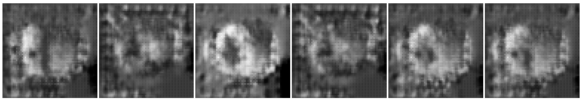
Blurry generated images with mode collapse visible.

Figure 15.
Augmentation of a CNN with samples generated by the trained TransfGAN.

Figure 16.
Number of cluster for different thresholds.

Figure 17.
Mean spectra of the images from (a) TransfGAN with λG = 0.0001, λD = 0.0001 no extra training, (b) TransfGAN with λG = 0.00005, λD = 0.00005, no extra training, (c) TransfGAN with λG = 0.0005, λD = 0.0005 with extra training, (d) the real sidescan dataset.
Figure 17.
Mean spectra of the images from (a) TransfGAN with λG = 0.0001, λD = 0.0001 no extra training, (b) TransfGAN with λG = 0.00005, λD = 0.00005, no extra training, (c) TransfGAN with λG = 0.0005, λD = 0.0005 with extra training, (d) the real sidescan dataset.


Table 1.
Labeled classes and division into training and test set.
| Object Class | Example Snippet | Number in Training Set | Number in Test Set |
|---|---|---|---|
| Tire |  | 18 | 17 |
Table 2.
Parameters varied in the ray-tracing simulation.
| Parameter | Range |
|---|---|
| sinking depth | 0 m–0.15 m |
| flight height | 2 m–6 m |
| across track distance | 5 m–30 m |
| outer tire radius | 0.5 m–0.6 m |
| inner tire radius | 0.26 m–0.3 m |
Table 3.
Generator of the TransfGAN.
| Layer | Neurons | Kernel Size | Stride | Padding | Activation Function | Feature Map Dimension |
|---|---|---|---|---|---|---|
| Input | - | - | - | - | - | |
| Dense | 3456 | - | - | - | relu | |
| Reshape | - | - | - | - | - | |
| Conv2DTranspose | 384 | - | relu | |||
| BatchNormalization | - | - | - | - | - | |
| Conv2DTranspose | 192 | relu | ||||
| BatchNormalization | - | - | - | - | - | |
| Conv2DTranspose | 96 | relu | ||||
| BatchNormalization | - | - | - | - | - | |
| Conv2DTranspose | 1 | tanh |
Table 4.
Discriminator of the TransfGAN.
| Layer | Neurons | Kernel Size | Stride | Padding | Activation Function | Feature Map Dimension |
|---|---|---|---|---|---|---|
| Input | - | - | - | - | - | |
| Conv2D | 32 | leaky relu | ||||
| Dropout | - | - | - | - | - | |
| Conv2D | 64 | leaky relu | ||||
| Dropout | - | - | - | - | - | |
| Conv2D | 128 | leaky relu | ||||
| Dropout | - | - | - | - | - | |
| Conv2D | 256 | leaky relu | ||||
| Dropout | - | - | - | - | - | |
| Dense (real/fake) | 1 | - | - | - | sigmoid |
Table 5.
Labeled classes for the classification task and division into training and test sets.
| Object Class | Number in Training Set | Number in Test Set |
|---|---|---|
| Tire | 18 | 17 |
| Rock | 36 | 210 |
| Background | 36 | 210 |
Table 6.
CNN used for classification.
| Layer | Neurons | Kernel Size | Stride | Padding | Activation Function | Feature Map Dimension |
|---|---|---|---|---|---|---|
| Input | - | - | - | - | - | |
| Conv2D | 16 | relu | ||||
| BatchNormalization | - | - | - | - | - | |
| Conv2D | 16 | relu | ||||
| BatchNormalization | - | - | - | - | - | |
| MaxPooling | - | - | - | |||
| Conv2D | 32 | relu | ||||
| BatchNormalization | - | - | - | - | - | |
| MaxPooling | - | - | - | |||
| Dropout | - | - | - | - | - | |
| Dense | 100 | - | - | - | relu | |
| Dropout | - | - | - | - | - | |
| Dense | 3 | - | - | - | softmax |
Table 7.
Experiments for the synthetic augmentation of the training dataset with the TransfGAN.
| Experiment | ||
|---|---|---|
| no GAN | 0.6230 ± 0.0153 | 0.6238 ± 0.0134 |
| , , no extra training | 0.6322 ± 0.0173 | 0.6316 ± 0.0141 |
| , , no extra training | 0.6367 ± 0.0249 | 0.6351 ± 0.0208 |
| , , with extra training | 0.6368 ± 0.0227 | 0.6349 ± 0.0180 |
Publisher’s Note: MDPI stays neutral with regard to jurisdictional claims in published maps and institutional affiliations. |
© 2021 by the authors. Licensee MDPI, Basel, Switzerland. This article is an open access article distributed under the terms and conditions of the Creative Commons Attribution (CC BY) license (http://creativecommons.org/licenses/by/4.0/).
Share and Cite
MDPI and ACS Style
Steiniger, Y.; Kraus, D.; Meisen, T. Generating Synthetic Sidescan Sonar Snippets Using Transfer-Learning in Generative Adversarial Networks. J. Mar. Sci. Eng. 2021, 9, 239. https://doi.org/10.3390/jmse9030239
AMA Style
Steiniger Y, Kraus D, Meisen T. Generating Synthetic Sidescan Sonar Snippets Using Transfer-Learning in Generative Adversarial Networks. Journal of Marine Science and Engineering. 2021; 9(3):239. https://doi.org/10.3390/jmse9030239
Chicago/Turabian StyleSteiniger, Yannik, Dieter Kraus, and Tobias Meisen. 2021. "Generating Synthetic Sidescan Sonar Snippets Using Transfer-Learning in Generative Adversarial Networks" Journal of Marine Science and Engineering 9, no. 3: 239. https://doi.org/10.3390/jmse9030239
Note that from the first issue of 2016, this journal uses article numbers instead of page numbers. See further details here.