Propagation of Solitary Waves over a Submerged Slotted Barrier


Department of Hydraulic and Ocean Engineering, National Cheng Kung University, Tainan 701, Taiwan
*
Author to whom correspondence should be addressed.
J. Mar. Sci. Eng. 2020, 8(6), 419; https://doi.org/10.3390/jmse8060419
Submission received: 24 May 2020
/
Revised: 5 June 2020
/
Accepted: 6 June 2020
/
Published: 9 June 2020
(This article belongs to the Special Issue Waves and Ocean Structures)
Abstract
:In this article, the interaction of solitary waves and a submerged slotted barrier is investigated in which the slotted barrier consists of three impermeable elements and its porosity can be determined by the distance between the two neighboring elements. A new experiment is conducted to measure free surface elevation, velocity, and turbulent kinetic energy. Numerical simulation is performed using a two-dimensional model based on the Reynolds-Averaged Navier-Stokes equations and the non-linear k-ɛ turbulence model. A detailed flow pattern is illustrated by a flow visualization technique. A laboratory observation indicates that flow separations occur at each element of the slotted barrier and the vortex shedding process is then triggered due to the complicated interaction of those induced vortices that further create a complex flow pattern. During the vortex shedding process, seeding particles that are initially accumulated near the seafloor are suspended by an upward jet formed by vortices interacting. Model-data comparisons are carried out to examine the accuracy of the model. Overall model-data comparisons are in satisfactory agreement, but modeled results sometimes fail to predict the positions of the induced vortices. Since the measured data is unique in terms of velocity and turbulence, the dataset can be used for further improvement of numerical modeling.
1. Introduction
Coastal structures are typically employed to reduce wave energy so as to mitigate coastal hazards for protecting the local residence [1] and coastal species [2]. On designing the structure, not only providing strong protection for the shore but also involving environmentally-friendly consideration should be balanced. In recent years, submerged-type structures have been extensively considered as alternative choices [3,4] to enhance water exchange and retain natural coastal landscape for a recreational purpose. On the other hand, coastal structures may have permeable parts, which leads to attenuate additional wave energy through viscous dissipation within the porous media [5,6]. A typical permeable structure mostly consisted of rubble-mounted elements. However, permeable objects can be built using several impermeable parts with slots to vary the porosity, which is known as screen-type barriers [7,8]. The classic type of barrier feature is thin, rigid, vertical, perforated, and surface-piercing, which is beneficial to account for economic and environmental concerns.
As reviewed in Huang et al. [9], most available studies in the literature have focused on evaluating the hydraulic performance in terms of wave reflection (R), transmission (T), and dissipation (D) coefficients, where surface-piercing-type barriers received more attention than those of submerged-type ones. Wu and Hsiao [7] numerically investigated solitary waves over a submerged dual-slotted-barrier system using a well-validated wave model based on the Reynolds-Averaged Navier-Stokes equations (RANS) by providing a simple empirical formula for estimating RTD coefficients, where wave conditions and porosities of each barrier are considered as the primary parameters for the estimations. However, the flow fields of wave interactions with slotted barriers were studied sparsely. Although several numerical studies have provided simulated flow fields around slotted barriers [8,10], flow separation is one of the complicated phenomena in fluid mechanics and may not be able to be resolved accurately using numerical models unless the model has been rigorously validated through detailed model-data comparisons [11]. Using the particle image velocimetry (PIV), Liu and Al-Banaa [12] studied non-breaking solitary waves runup on a vertical surface-piercing barrier, and Wu et al. [13] investigated breaking solitary waves over a submerged bottom-mounted barrier. However, the flow fields due to the interaction of solitary waves and a submerged slotted barrier were not understood.
In practical applications, the elements of slotted barrier can be installed either horizontally or vertically, and, thus, the problem to be solved results in two-dimensional and three-dimensional setup for horizontal and vertical slotted barriers, respectively. Thomson [14] stated that the orientations of slotted barriers had an influence on transmitted waves based on experimental observation, where the horizontal slotted barrier appeared to be more effective in reducing wave transmission. In addition, choosing the shape of slotted barriers is one of the factors affecting the hydraulic performance. Krishnakumar et al. [15] stated that the slotted barrier with sharp edge elements such as square, rectangle, and triangle result in lower wave transmission but higher wave reflection than those consisting of circular shape elements. Additionally, Huang et al. [9] indicated that the rectangular element of perforated barriers may help generate more energy dissipation due to flow separation around the sharp edge elements of slotted barriers. Therefore, based on statements mentioned in available literature, the horizontal slotted barrier with rectangular elements may be the optimized setup as effective coastal structures, which can be considered a two-dimensional (2D) problem.
In this study, the primary aim is to investigate and understand the flow fields of solitary waves interacting with a submerged slotted barrier experimentally and numerically. A new experiment is performed in a laboratory-scale wave flume to measure the free surface displacement time series, the ensemble-averaged flow velocities, and the turbulent kinetic energy. Numerical simulation is carried out based on the RANS equations for the mean flow fields and the non-linear k-ɛ turbulence closure model to approximate the Reynolds stresses [16,17]. Detailed flow fields are addressed based on laboratory observations. Model-data comparisons in terms of the free surface elevation time series, the mean velocities, and the turbulent kinetic energy are performed to examine the accuracy of the numerical model and point out the limitation of numerical simulations.
2. Research Methods
2.1. Experiment
An experiment was conducted in a 2D glass-walled and glass-bottomed wave flume, which allowed the use of optical-based and image-based measuring systems. The flume dimensions are 22.0 m long, 0.50 m wide, and 0.76 m deep, located at Tainan Hydraulics Laboratory, National Cheng Kung University, Taiwan. A computer-controlled piston-type wavemaker was installed at one end of the flume and a sloping beach with a layer of concrete units was constructed at the other end to dissipate the transmitted wave energy. The slotted barrier was designed with an overall dimension of 10 cm high and 2 cm thick, which is identical to the study of a solid barrier under solitary waves [13], and was consisted of three identical square elements with a dimension of 2 cm × 2 cm made by transparent acrylic units. Therefore, the resulting porosity of the slotted barrier is 0.40. The slotted barrier was suspended in the wave flume with 2 cm freely from the top of the structure to the free surface and from the lower end of the barrier to the seafloor. The slotted barrier was installed around the middle of the flume at the constant water depth region, where the water depth h is 14 cm. Two different wave heights H were considered in the experiment for which H/h = 0.29 and 0.18.
Figure 1 shows the experimental layout, apparatus, definitions of variables used in this study and flowchart for instrument synchronization. Four capacitance-type wave gauges were employed to measure the free surface elevation time series in which two of them were positioned in front of the slotted barrier for recording incident and reflected waves, and the other two are instrumented behind the barrier for measuring transmitted waves. All wave gauges were synchronized with the wavemaker for 60-s recording with a sampling rate of 100 Hz. The first wave gauge (WG1) was used to define the wave height and reference the time origin as the wave crest passing over this wave gauge. The origin of the coordinate system (x, z) = (0, 0) was defined at the intersection of the seafloor and the leading edge of the submerged slotted barrier.
Flow velocities were measured by a time-resolved PIV system, which consisted of a high-speed camera and a continuous laser [18]. Instantaneous particle images were captured by an 8-bit digital CMOS camera (MS55K2, Canadian Photonic Labs Inc) with a resolution of 1280 × 1020 pixels and a maximum 1,000 framing rate per second (fps). Images were captured by using an in-house software of the camera, which was also used in Reference [19], and the camera was triggered by an external signal from the wavemaker. A single field of view (FOV) that covered an area of 239.2 mm × 190.6 mm in the vicinity of the slotted barrier (see Figure 1 for relative location) was used. A 2w continuous laser was employed as a light source to illuminate the measuring region. The frame rate of the PIV system was set to 200 fps and, thus, the temporal resolution of the velocity field was 199 fps while a 50-fps recording was set for flow visualization, which provides the path line of the flow fields to help identify the induced vortices qualitatively. Since the same PIV system with a similar setup has been used, the estimation of uncertainty for velocity determination can be referred to Reference [20]. Raw PIV images were processed using a multi-pass algorithm [21]. The analyses were starting from 128 × 128 pixels and ending with 32 × 32 pixels with a 50% overlap. Spurious velocity vectors were removed from the cross-correlated velocity fields using a dynamic mean value filter and a local median filter (3 × 3 vectors) [22]. No attempt was made to smooth or interpolate the cross-correlated velocity fields. The experiments were repeated under identical initial and boundary conditions up to 20 and 10 times for the cases of H/h = 0.29 and 0.18, respectively. The Reynolds-decomposition method was used to obtain the ensemble-averaged free surface elevation and the flow velocity. Due to the limited repeated runs, the turbulent kinetic energy could only be estimated for the case of H/h = 0.29.
2.2. Numerical Model
In recent years, the RANS-type model has been extensively used in coastal and ocean engineering applications, such as tsunami runup [23,24], wave-current interactions [25], and waves interacting with structures [26,27]. In this study, a 2D depth-resolving and phase-resolving viscous numerical wave model is used to simulate the interaction of a solitary wave and a submerged slotted barrier. The physics behind the model is based on the RANS equations to describe the mean flow fields and the non-linear k-ε closure model to approximate the Reynold stresses by means of the turbulent kinetic energy (k) and the turbulent dissipation rate (ε). The model solves the RANS equations by using the finite-difference two-step projection method [28]. The free surface displacement during wave-structure interactions is traced by the volume of fluid method [29]. The no-slip condition is implemented at the solid boundaries and the zero-stress condition is applied to the mean free surface for neglecting the air-flow effect. The surface tension is not considered in this study. Solitary waves, where the wave conditions are identical to those of experiments, are generated through the inflow boundary by giving the theoretical solutions [30] in terms of free surface displacement along with the corresponding horizontal and vertical velocities. The radiation boundary condition is utilized for allowing the wave outgoing the computational domain to eliminate significant reflection. More detailed information about the numerical implementation can refer to References [16,17]. The model used in this study has been rigorously validated against experimental measurements in terms of velocity and turbulence for coastal-related problems such as solitary wave interactions with a submerged impermeable breakwater [31], submerged permeable structure [5], surface-piercing barrier [12], and submerged bottom-mounted barrier [13]. However, the flow-field accuracy for solitary wave interactions with a slotted barrier, especially focusing on flow separations, has not been investigated yet.
The numerical setup used herein can be very similar to the studies of solitary waves interacting with a bottom-mounted barrier [13] and dual-solid-barrier [7]. However, the wave-induced flow fields are much more complicated due to flow separation that occurs by each element of the slotted barrier. Furthermore, those induced vortices are expected to interact with each other to further create a complex flow pattern like the vortex shedding process [32]. As a result, such complicated phenomena are very difficult to accurately simulate. The flow separation is closely linked and inseparable from the development of the boundary layer flow, especially near the surfaces of the bottom boundary and the object elements. Typically, to avoid tremendous computational efforts, the RANS model always employed a log-law model to simplify the boundary layer flow using a logarithmic velocity profile because the tiny thickness of the boundary layer may not be able to be directly resolved, especially for the wave condition with a high Reynolds number. However, such simplification may lead to inaccurate results in the vicinity of flow separation regions under wave actions [31]. The laminar boundary layer characteristics under solitary waves can be estimated from the formula derived by Reference [33] and later improved by Reference [34]. The estimated boundary layer thickness (BLT) is expressed as:
in which C is the wave celerity of a solitary wave, KC is to estimate the duration of a solitary wave, and υ is the kinematic viscosity of the fluid. According to Equation (1) with h = 14 cm, the estimated BLT for the case of H/h = 0.29 is around 1.0 mm whereas, for the case of H/h = 0.18, the estimated BLT is around 1.1 mm. The higher the H/h, the thinner the estimated BLT. Following Reference [34] for the treatment of solid boundaries, the region within 0 ≤ z/BLT ≤ 5 is resolved by 20 grids whereas the region within 5 ≤ z/BLT ≤ 10 is resolved by 10 grids with uniform distributions of numerical meshes. By doing this, for the case of H/h = 0.29, the minimum resolution is set to 0.25 mm. After performing sensitivity analyses on the use of different grid resolutions, it is found that the modeled results for the region within 0 ≤ z/BLT ≤ 10 resolved by 40 grids and more grids are almost the same, so that the results presented in this study employ 40 numerical grids to resolve 10 times of the estimated BLT for all solid boundaries, including the seafloor and the surfaces in the vicinity of each element of the slotted barrier. The computational domain is designed as −2.5 m ≤ x ≤ 2.4 m and 0.0 m ≤ z ≤ 0.2 m, where the origin is defined at the weather side of the slotted barrier like the definition used in the experiments.
3. Results and Discussion
3.1. Free Surface Elevation
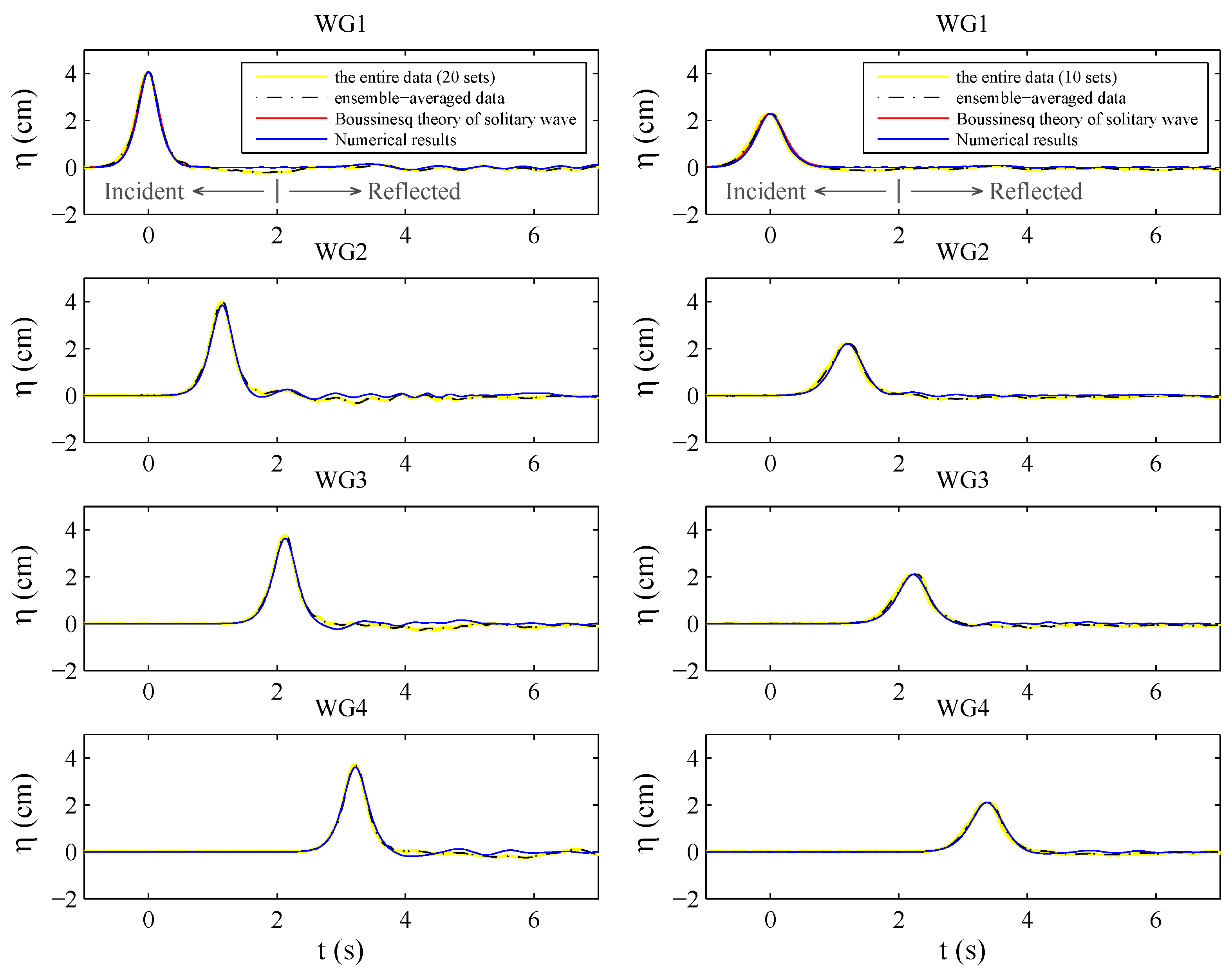
To verify the initial force of solitary waves, comparisons between experimental measurements and numerical simulations are performed for time histories of the free surface elevations at selected locations. Figure 2 shows the model-data comparisons for four wave gauges (see Figure 1 for relative locations) where the left and right columns demonstrate the results obtained from the cases of H/h = 0.29 and 0.18, respectively. Since the numerical wave tank is shorter than that of the physical experiment, numerical wave heights are decided by matching the measured wave heights at WG1, where the time origin is also referenced. For experiments, all instantaneous measurement and mean free surface elevations are plotted in the same figure for each position of wave gauges. All measured data almost overlap with each other and show the high repeatability of experiments. Quantitatively, the standard deviation for incident wave heights obtained from all 20 trials for the case of H/h = 0.29 is around 0.2 mm while the standard deviation for the case of H/h = 0.18 obtained from 10 repetitions is less than 0.1 mm. This, once again, indicates the high repeatability of the present experiments. In addition, model-data comparisons reveal that numerical calculations for both wave conditions fit the measurements well for the main waveforms in terms of incident and reflected waves recorded by WG1 and WG2 and transmitted waves recorded by WG3 and WG4. Moreover, the theoretical solutions of the solitary wave [30] are also plotted at WG1 of Figure 1 for both cases. It is evident that comparisons show satisfactory agreements between theoretical, measured, and model waveforms of solitary waves. Furthermore, the wave transmission coefficients (CT) can be simply calculated by the wave height ratio, which is obtained from WG4 and WG1. The estimated CT was around 0.86 and 0.83 for the cases of H/h = 0.29 and 0.18, respectively.
3.2. Flow Visualization
Resolving the generation and evolution of vortices at the initial stage of flow separation relies on a very high-resolution PIV system, as the scale of those vortices are too small to be fully resolved and the velocities there are also small compared to the velocities due to pure wave actions. Some previous studies [35,36] have raised the same difficulty, so that further efforts on quantitating those tiny vortices are necessary. To provide a better understanding of the flow separation induced flow fields, a flow visualization technique was used to qualitatively define the flow characteristics. The particle tracking technique was employed for flow visualization by carefully adjusting the camera exposure to generate path lines of the induced flow pattern. The size of FOV for using the particle tracking technique is identical to that used in the PIV measurement. However, the temporal resolution is reduced to 50 fps. Although the induced flow fields for those of two wave conditions reveal different strengths and movements of induced vortices, the overall phenomena in terms of the flow pattern are nearly the same. Therefore, only the flow visualization for the case of H/h = 0.29 is presented herein and their differences of varying wave conditions are provided by means of a model-data comparison for velocity fields.
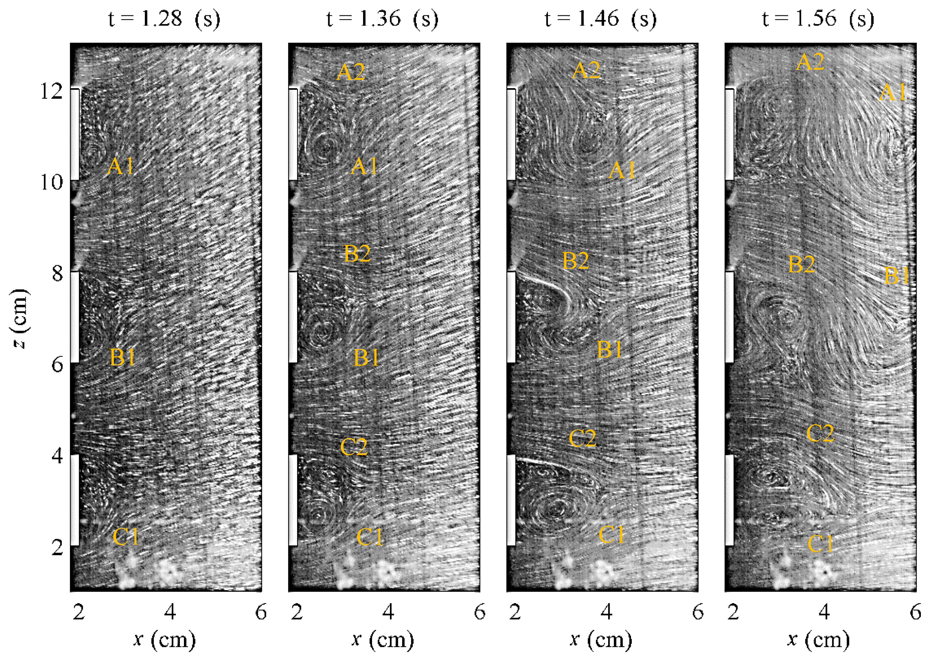
Flow visualization images were re-sized in order to better demonstrate those tiny vortices due to flow separation. Figure 3 shows a close view for the initial stage of flow separation while Figure 4 and Figure 5 show the stage of the vortices’ interaction. Based on laboratory observations, the phenomena of flow separation occurred at both sides of each element and, for all three elements of the slotted barrier, the vortices in the lower end of the element are induced first and the vortices in the upper side of the element are induced later. This may be partly due to the slight pressure difference between the upper and lower parts of the element. The lower part has relatively large hydrostatic pressure whereas the upper side suffers a relatively low pressure. The induced vortices are labelled in Figure 3, Figure 4 and Figure 5 and the rule for labelling vortices is followed. The upper, middle, and lower elements are, respectively, named as A, B, and C, and the sequence of induced vortices are numbered. For example, the first vortex induced by the first element is labelled as A1.
As shown in Figure 3 at t = 1.28 s, distinct vortices are visible at the lower end of the elements, i.e., A1, B1, and C1. At t = 1.36 s, the size and its strength of the lower vortices gradually increase and then the vortices induced by the upper sides of the elements, i.e., A2, B2, and C2, are generated slightly later, where their sizes are smaller and strengths are weaker than those of A1, B1, and C1. At t = 1.46 s, the vortices A1 and B1 convect downstream and its pathline is cut out by the vortices induced by the upper end of the elements, i.e., A2 and B2, and new vortices are then generated from the edges of the elements due to flow separation. Such phenomena of vortices’ interaction are like the vortex shedding process of uniform flow passing through an obstacle [32]. Moreover, it is found that the time instant of shedding out of the vortices induced by the lower end of the elements is different. As can be seen at t = 1.56 s, the vortex A1 sheds out of the vortex street first. This is followed by B1. The vortices induced by the lowest element form a pair of almost symmetric vortices, i.e., C1 and C2, with different rotating directions.
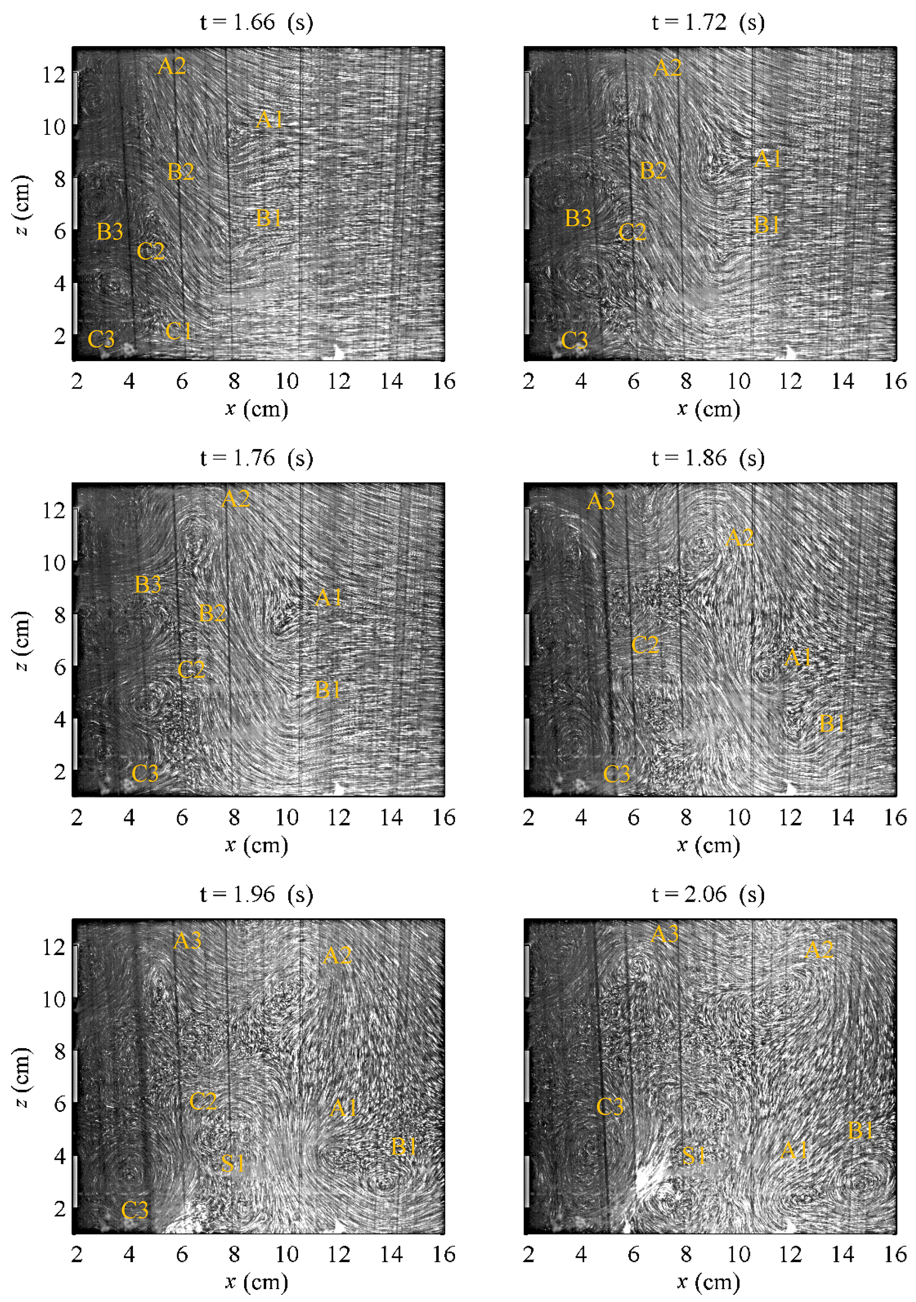
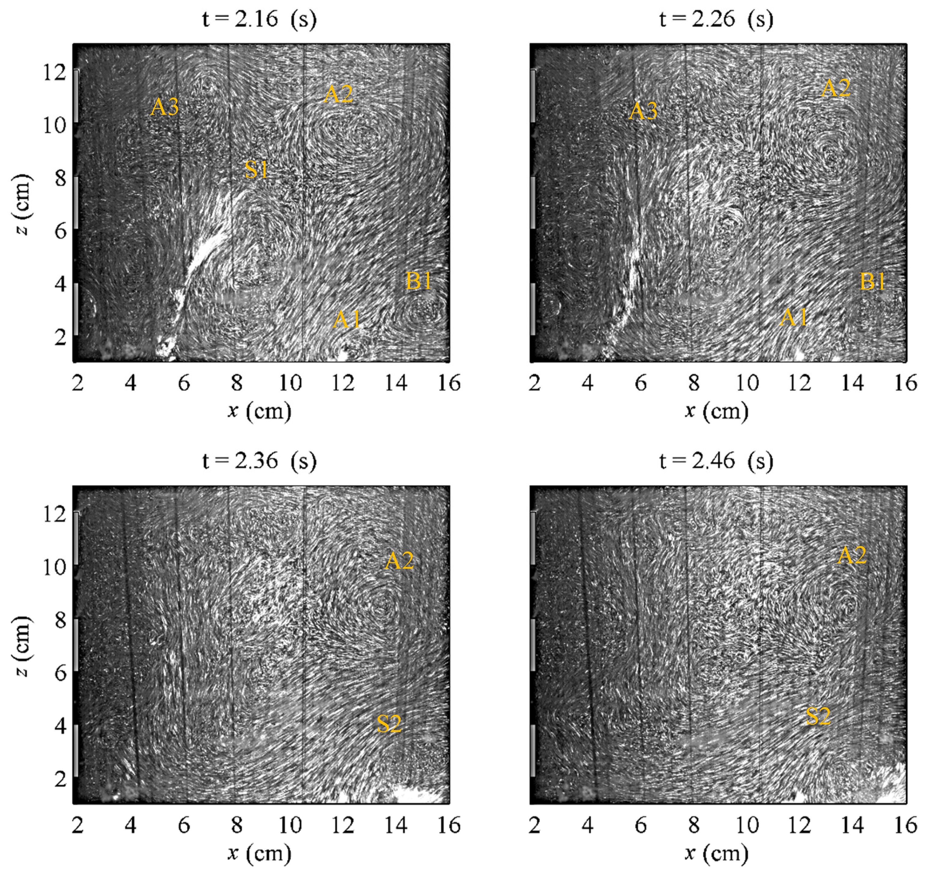
In Figure 4, before t = 1.56 s, the flow is dominated by the acceleration part of the solitary wave, i.e., before the arrival of the wave crest. After t = 1.56 s, the deceleration part of the solitary wave then passes over the slotted barrier. As t = 1.66 s to 1.72 s, the vortices A1 and B1 move downward due to the decrease of the free surface. Then, until t = 2.06 s, those two vortices move downward to the bottom and eventually merge together to form a distinct counterclockwise vortex due to the same rotating direction, i.e., t ≥ 2.36 s in Figure 5. In between t = 1.66 s to 1.86 s, the vortices A2, B2, and C2 are then shed out of the vortex street to further induce vortices. Vortex A2 moves upward to reach the free surface. Vortices B2 and C2 also slightly move upward and then eventually diffuse due to the complicated vortices’ interaction. In addition, a distinct vortex A3 is later induced by the first element with a clockwise rotation, i.e., at t = 1.86 s, and a counterclockwise-rotating vortex C3 occurs by the lowest element. At t = 1.96 s, a clockwise-rotating vortex is generated due to the viscous effect of the bottom boundary, i.e., S1. Then, a strong upward vertical velocity is visible at t = 2.06 s due to the opposite rotating directions between C3 and S1, which indicates possible sediment suspension of the seafloor. In Figure 5, a considerable amount of seeding particles originally accumulated near the bottom is suspended upward due to the strong vertical velocity gradient at t = 2.16–2.26 s. Furthermore, the vortex S2 merged from A1 and B1 may also lead to sediment suspension at t = 2.36–2.46 s. In practical engineering using submerged breakwaters, the scour of seafloor is mostly found near the toe of the breakwater. However, in this study, possible scour by means of seeding particle suspension is found in the shoreward direction. It will be interesting and of great importance as an extended work to conduct a mobile seabed experiment for the same obstacle setup.
3.3. Velocity Fields
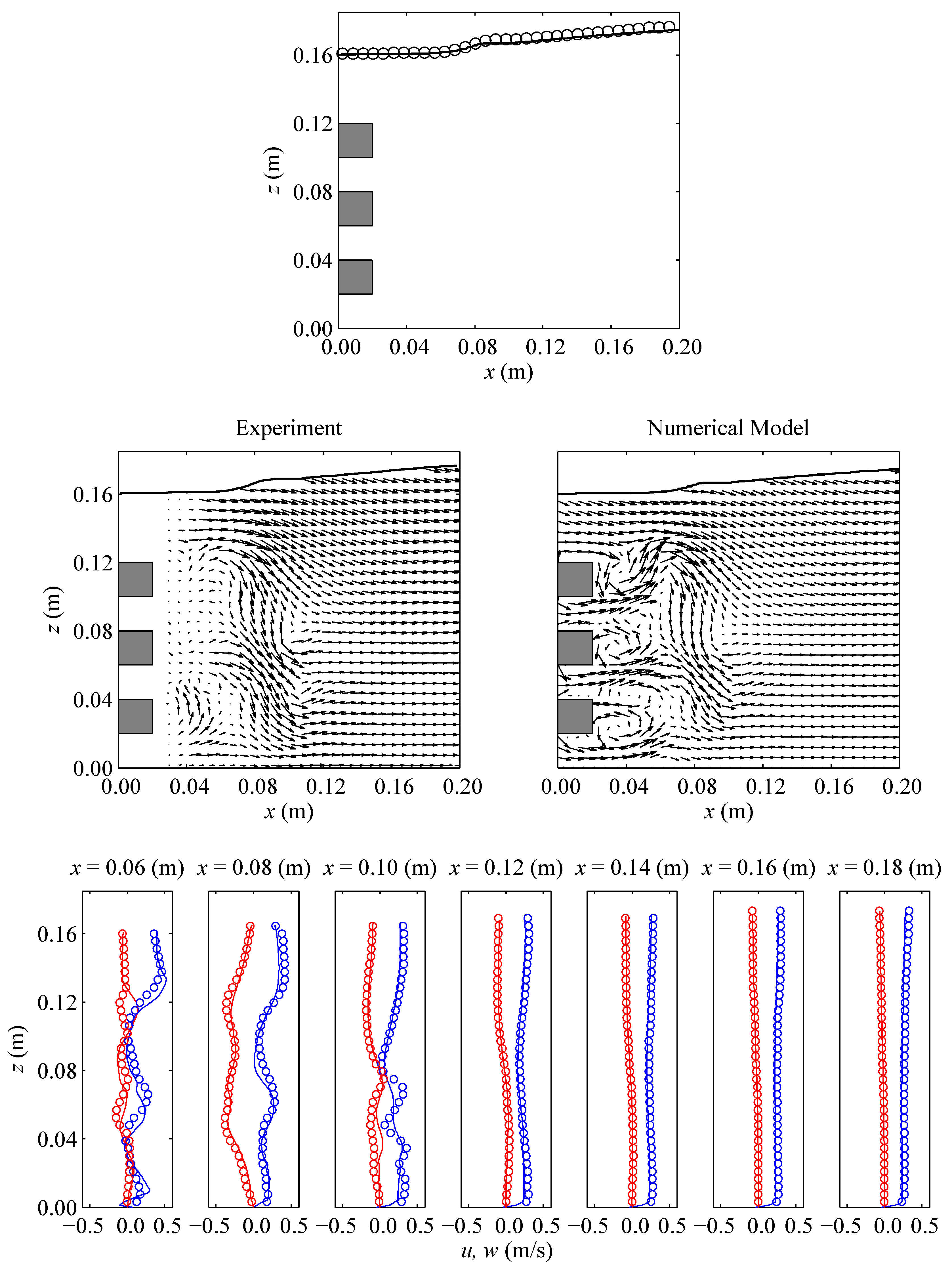
Given that free surface deformations are clearly illuminated by a laser and imaged by the PIV camera, the free surface displacements can be detected and used for model-data comparisons in spatial variations. Figure 6, Figure 7, Figure 8, Figure 9 and Figure 10 present detailed model-data comparisons in terms of spatial distribution of free surface elevation (top column), velocity fields (middle column), and corresponding velocity profiles in both horizontal and vertical components (lower column) for the cases of H/h = 0.29 (Figure 6, Figure 7, Figure 8 and Figure 9) and H/h = 0.18 (Figure 10). For velocity profiles, seven cross-sections are uniformly selected from x = 0.06 m to x = 0.18 m with an identical interval of 0.02 m. It is remarked in these cases that the selected locations of velocity profiles may not be the same between experiments and numerical modeling because their resolutions in space are essentially different. As such, the closest locations between measurements and simulations are selected for comparisons, and no interpolation of the results is attempted. Since the laser was illuminated from the bottom of the flume, those near each element of the slotted barrier and free surface may not be well-illuminated, so that those data have been removed in order to avoid providing inaccurate velocity information.
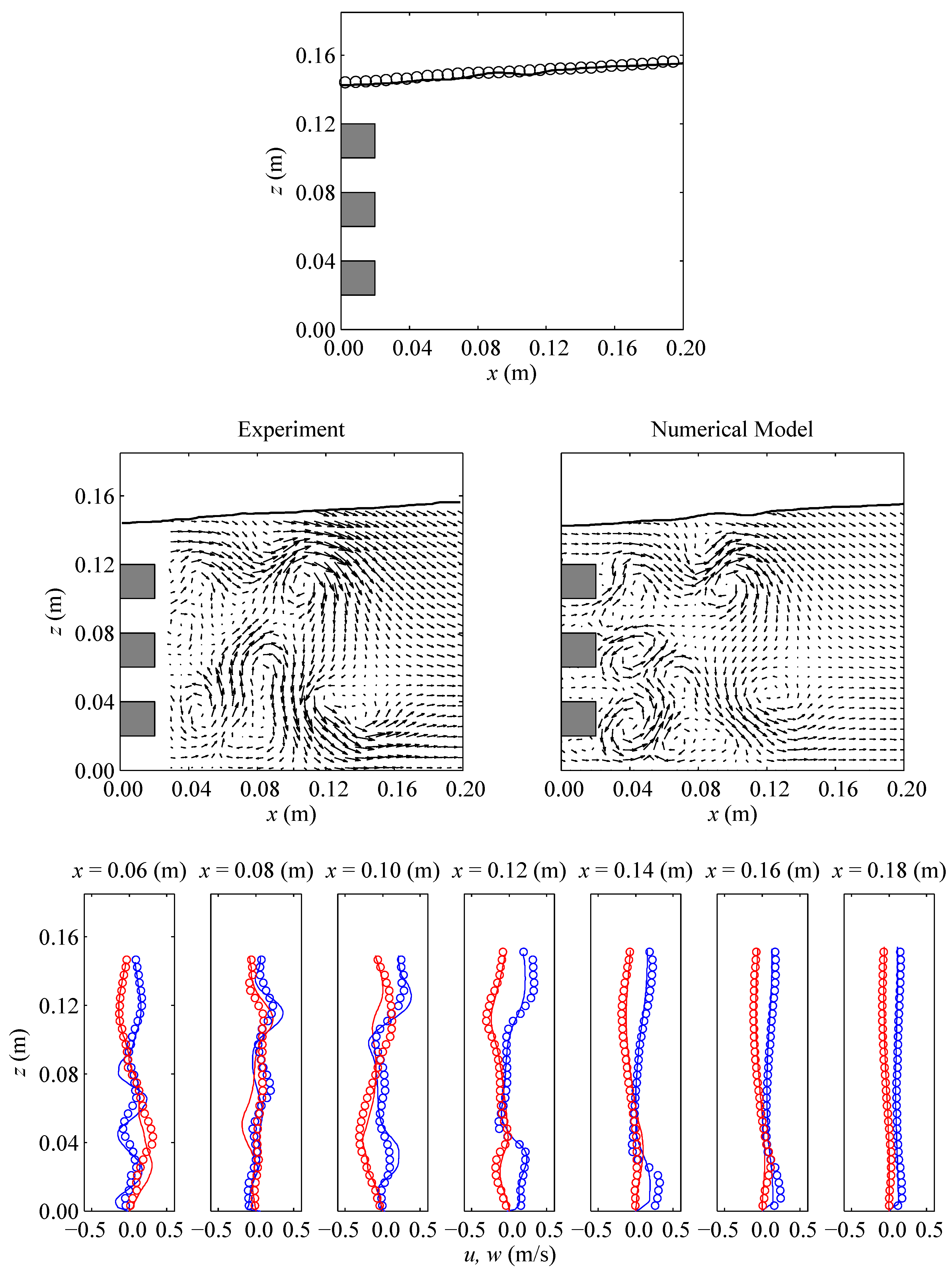
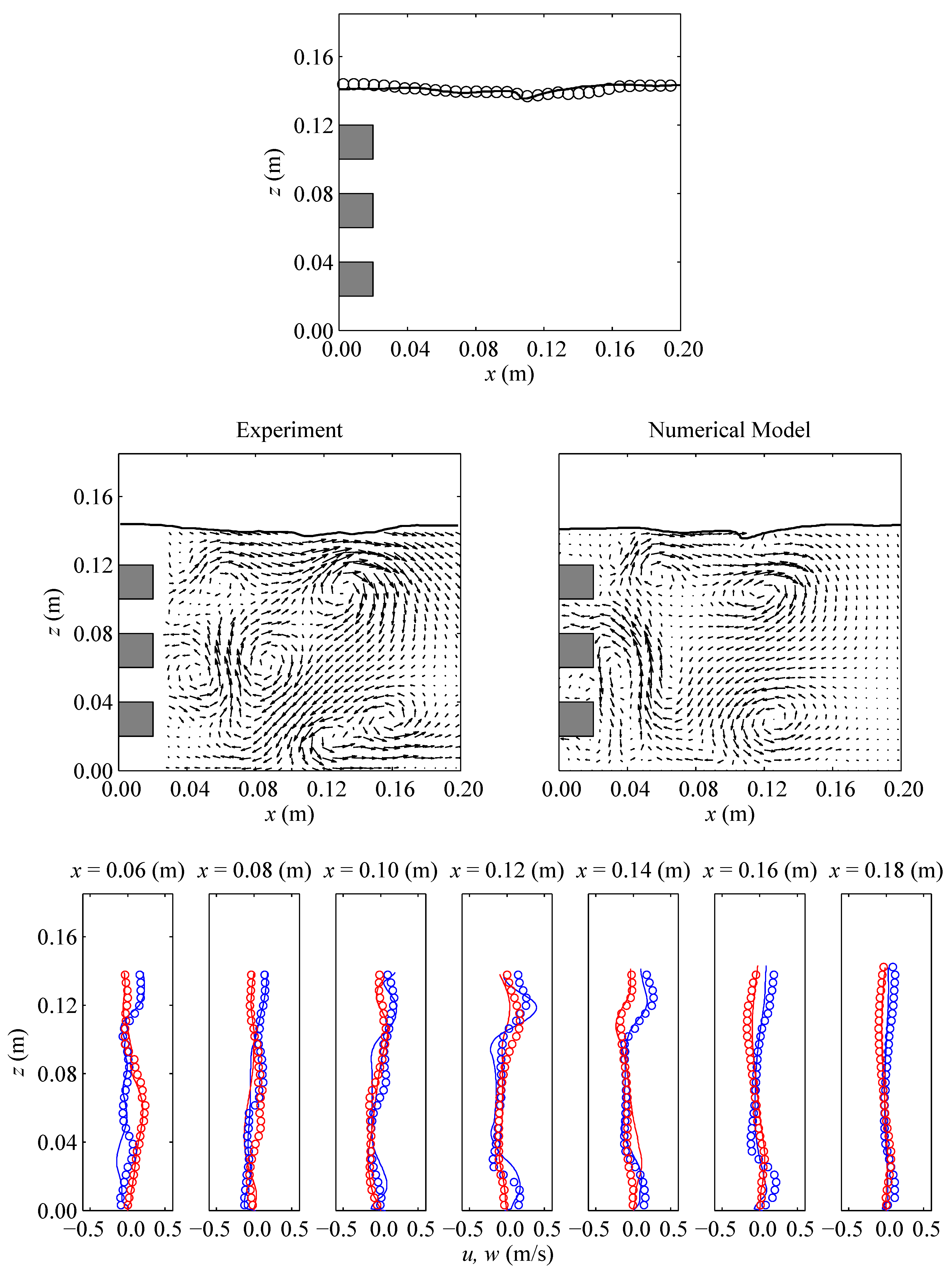
Figure 6 shows the time instant that the solitary wave crest is at the leading edge of the slotted barrier, belonging to the initial stage of flow separation. In Figure 7, the crest of the solitary wave has entirely passed over the slotted barrier and the velocity fields reveal the start of the vortex shedding process. The physical phase for the interaction of vortices is demonstrated in Figure 8. Distinct vortices A1, A2, A3, B1, C2, C3, and S1 are clearly visible and resolved by PIV measurements and RANS simulations. Figure 9 demonstrates the time instant of the strong upward velocity like a vertical jet shot from the bottom, which causes significant seeding particles suspended. These are initially accumulated near the seafloor. Model-data comparisons show that the free surface deformation during the interaction of a solitary wave and a submerged slotted barrier can be well-captured by the present RANS model, where the wave heights and phases at different time instants show satisfactory agreements. However, for the velocity fields, modeled results at some points fail to fit measured data. More specifically, the modeled results fit the measurements very well at the initial stage of flow separation, as shown in Figure 6 and Figure 7. Significant discrepancies are observed during the vortex shedding process, which can be seen in Figure 8 and Figure 9, and can be summarized into three main reasons. First, the positions of the induced vortices between the physical experiment and numerical model are not always the same, which causes significant variations after complicated vortices interact. Second, the vortices A1 and B1 at t = 2.16 s are not yet merged into a distinct vortex S2 in the measurement whereas the numerical results show those two vortices have been merged already at that time instant (see Figure 9). Third, it seems that the modeled flow fields are affected by the deceleration part of the solitary wave more than those of experiments, so that the entire flow fields are somewhat shifted to the opposite direction of the propagating wave (see Figure 8 and Figure 9). Except those discrepancies, model-data comparisons are generally in satisfactory agreements. The main feature of the flow pattern can be simulated well by the model, including the initial stage of flow separation, an overall vortex shedding process, and an upward vertical velocity due to the interaction between vortices C3 and S1, which may further trigger sediment suspension locally.
Another model-data comparison is made for the case of H/h = 0.18. Since the overall flow pattern is mostly identical to the case of H/h = 0.29, only a few stages are slightly different from those of H/h = 0.29. As such, only one time instant for a model-data comparison is provided. Experimentally, one of the variations of varying wave conditions is that the time instant for merging vortices A1 and B1 into S1 is earlier than the case of H/h = 0.29. Figure 10 shows the time instant at t = 2.32 s, which is 0.6 s behind the wave crest arriving at the leading edge of the slotted barrier. The two vortices A1 and B1 have merged into a distinct vortex S1. In addition, the upward vertical jet is much closer to the barrier than the case of H/h = 0.29, which is around 0.04 m and 0.06 m for the cases of H/h = 0.18 and H/h = 0.29, respectively. In addition, modeled results again fit the measured data well for overall comparisons, but some detail flow fields cannot be simulated well, especially for the positions of the induced vortices and their sequential interactions. One of the reasons may be due to the use of a two-equation turbulence model, which may be oversimplified for representing the effects of turbulent flow fields. RANS equations with a two-equation turbulence closure model is useful for practical applications [37], as only mean flow fields are simulated. However, detailed flow fields due to complicated wave-structure interactions may not be accurately simulated. Various efforts have been made using different approaches prior to demonstrate the simulations presented herein, such as employing very fine mesh to resolve the flow characteristics near the solid boundaries instead of using the log-law approach. As one of the ongoing works, further attempts may be considered using different two-equation turbulence models, such as those used in Reference [37], and various concepts of turbulence representation, such as a LES (large-eddy-simulation) model [38].
3.4. Turbulent Kinetic Energy
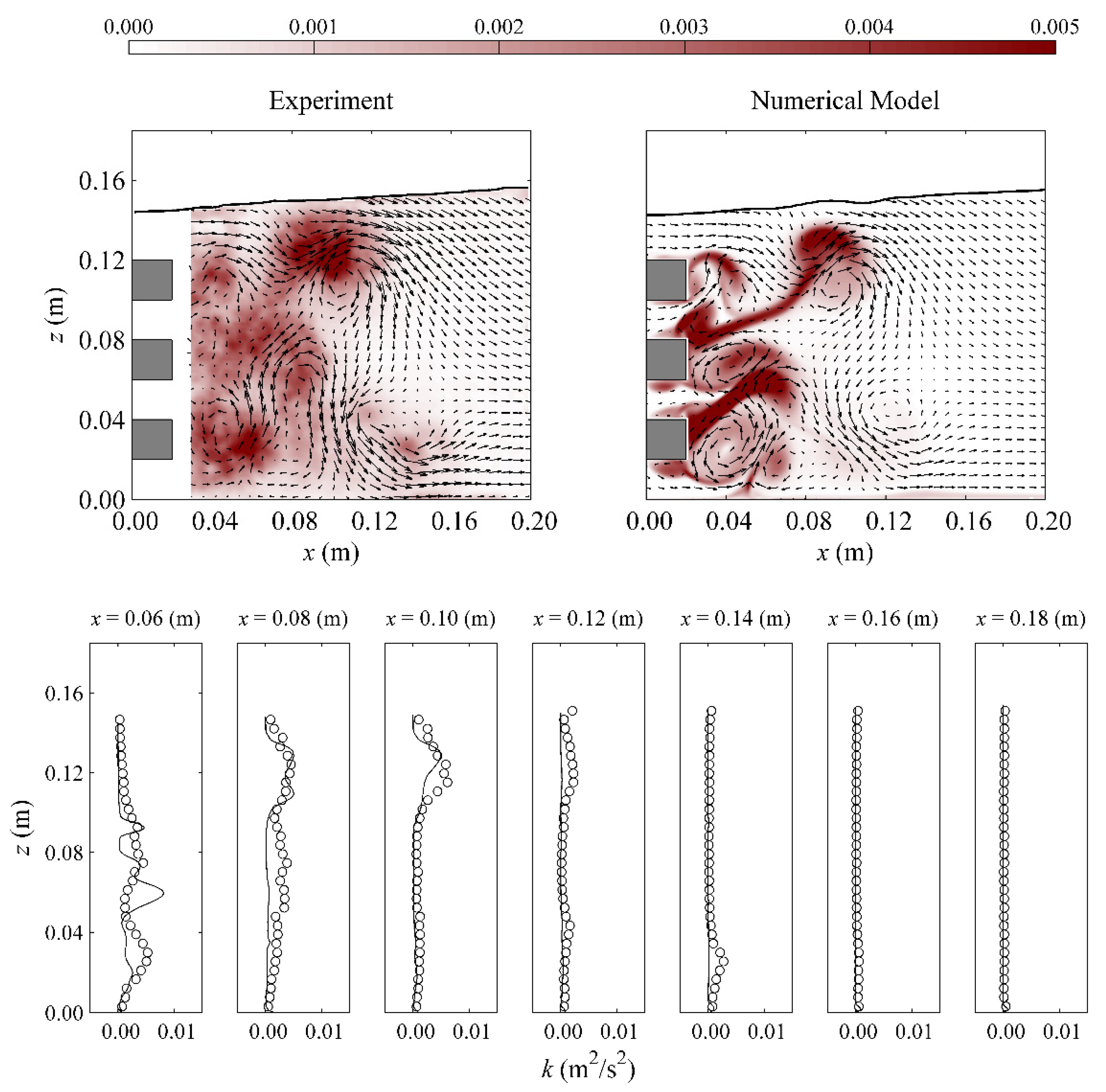
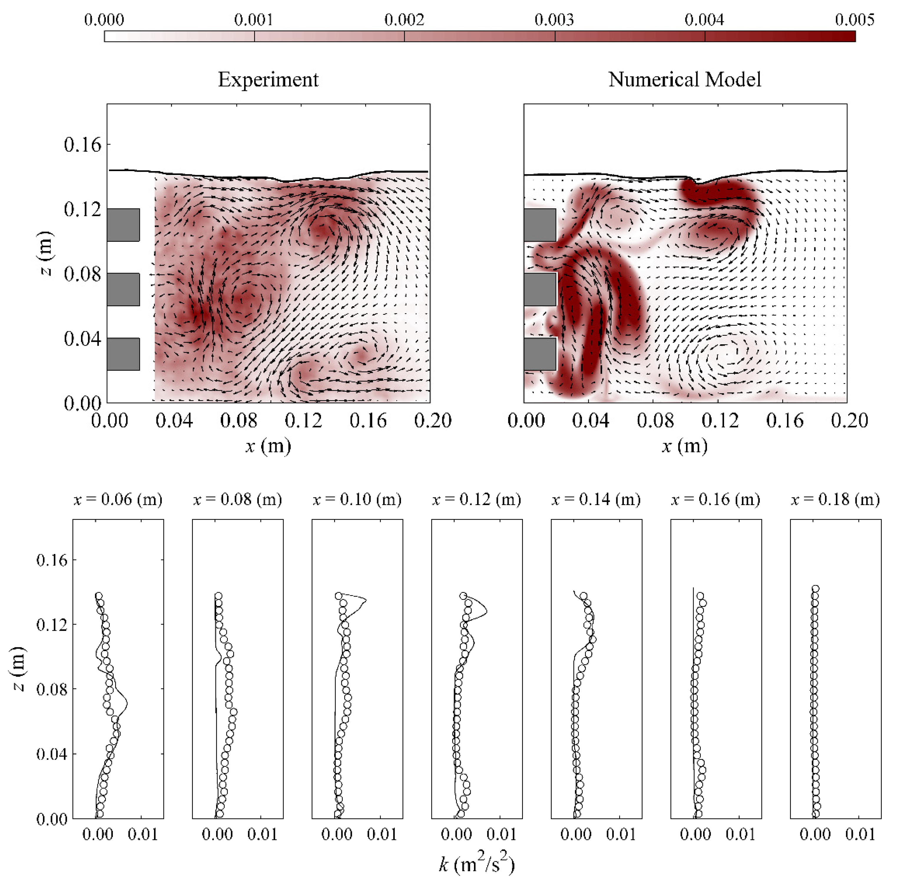
According to References [39,40], meaningful turbulence characteristics can be estimated through ensemble averaging over 16 or more repetitions of the same experiments under identical initial and boundary conditions. As a result, only the case of H/h = 0.29 can be used to estimate the turbulent kinetic energy based on measured velocity information. Detailed information on how to obtain turbulence characteristics can be found in References [5,12,13,39,40]. Model-data comparison in terms of spatial distribution of turbulent kinetic energy (TKE) and its corresponding cross-sections is presented, where the profile locations of TKE are identical to those of velocity fields. Since TKE generation and evolution at the initial stage of flow separation are surrounded by each element of the slotted barrier also in order to reduce the number for figures, only the time instants showing significant TKE evolution, i.e., t = 1.96 s and 2.16 s, are demonstrated and the other physical phases are described concisely. In Figure 11 and Figure 12, the TKE fields are superimposed with velocity maps to help identify the locations of induced vortices and TKE.
At the initial stage of flow separation, TKE is generated from the slots of two neighboring elements with a local maximum TKE around 0.005 m2/s2 for both measured and modeled results. At t = 1.76 s, the measured local maximum TKE induced by vortices A2 and B2 are around values of 0.006 m2/s2 and 0.005 m2/s2, respectively, whereas the modeled TKE induced by vortices A2 and B2 are around values of 0.005 m2/s2 and 0.002 m2/s2, respectively. As shown in Figure 11, the local maximum TKE is introduced by vortex A2 with a value of around 0.006 m2/s2 for measurement and around 0.005 m2/s2 for simulation. Another important phase of TKE is due to the upward vertical jet at t = 2.16 s, as shown in Figure 12, where the measured and modeled local maximum TKE are around 0.005 m2/s2 and 0.006 m2/s2, respectively. As mentioned in the previous section, the locations of induced vortices between measured and modeled results are not identical, which are also shown for the vortices induced by TKE, so that it is more appropriate to find a local maximum value of a specific vortex for a model-data comparison. Detailed comparisons are made for cross-section TKE. In general, the overall trend of TKE profiles fits the measurements with reasonable agreement.
4. Conclusions
In this study, the interaction of solitary waves and a submerged slotted barrier was investigated experimentally and numerically. An experiment was conducted to measure free surface elevations using wave gauges and velocity fields using a time-resolved PIV. A 2D depth-resolving and phase-resolving wave model based on the 2D RANS equations and the non-linear k-ε turbulence closure model was employed to reproduce the experiments.
Due to the highly complex nature of flow fields from wave-structure interactions, flow visualization was also utilized to help identify the detailed flow characteristics of tiny vortices that may not be measured using present PIV. Numerically, very fine meshes were used to resolve the velocities near all solid boundaries instead of using a log-law approach. Model-data comparisons were performed in terms of free surface elevation, velocity, and turbulence characteristics. Overall, the comparisons were in satisfactory agreements. Expect few inaccurate predictions for the positions of induced vortices. Since most of the existing literature paid attention to evaluating the hydraulic performance of slotted barriers, to the best knowledge of the authors, no available study provides the detailed velocity and turbulence information of a slotted barrier under a water wave. This is the first dataset providing detailed measurements on solitary wave interactions with a submerged slotted barrier, which can be used as a benchmark case for further development of the numerical model and for model validation.
According to laboratory observations, the flow separation of each element of the slotted barrier and the vortex shedding process was triggered due to the interaction of those induced vortices to generate a complicated flow pattern. It was also found that, for this setup, an upward vertical velocity with a significant strength of velocity and turbulence was qualitatively observed and quantitatively measured, which showed a large number of suspended seeding particles. These were originally accumulated near the seafloor. This indicates that there may be potential scouring near the submerged slotted barrier and this may result in a local geometry change. Numerical simulation also confirmed those findings. As part of ongoing work, it will be interesting to conduct a mobile seabed experiment for a submerged slotted barrier under a solitary wave to investigate the possibility of scouring the seafloor. In addition, only one obstacle setup was considered in the experiment. The gap of each element and the designed water depth may also be critical factors affecting the formation of velocity fields as well as the vortex shedding process, which should be worthy of investigation.
Author Contributions
Y.-T.W. and S.-C.H. conceived the research topic. Y.-T.W. performed experiments, numerical simulations, and data analyses. Y.-T.W. and S.-C.H. wrote the paper. All authors have read and agreed to the published version of the manuscript.
Funding
The Ministry of Science and Technology, Taiwan (MOST 108-2218-E-006-053-MY3, 108-2221-E-006-087-MY3) and the Water Resources Agency of Ministry of Economic Affairs, Taiwan (MOEAWRA1090350) funded this research. Yun-Ta Wu appreciates the support of the Open Fund Research SKHL1813 of Sichuan University for a short-term visit in 2019.
Acknowledgments
The author sincerely appreciates the staffs of Tainan Hydraulics Laboratory of NCKU for their help in conducting the experiments.
Conflicts of Interest
The authors declare no conflict of interest.
References
- Strusińska-Correia, A. Tsunami mitigation in Japan after the 2011 Tōhoku tsunami. Int. J. Disaster Risk Reduct. 2017, 22, 397–411. [Google Scholar] [CrossRef]
- Ware, M.; Long, J.W.; Fuentes, M.M.P.B. Using wave runup modeling to inform coastal species management: An example application for sea turtle nest relocation. Ocean Coast. Manag. 2019, 173, 17–25. [Google Scholar] [CrossRef]
- Lara, J.L.; Garcia, N.; Losada, I.J. RANS modelling applied to random wave interaction with submerged permeable structures. Coast. Eng. 2006, 53, 395–417. [Google Scholar] [CrossRef]
- Kobayashi, N.; Meigs, L.; Ota, T.; Melby, J. Irregular breaking wave transmission over submerged porous breakwater. J. Waterw. Port Coast. Eng. 2007, 133, 104–116. [Google Scholar] [CrossRef]
- Wu, Y.-T.; Hsiao, S.-C. Propagation of solitary waves over a submerged permeable breakwater. Coast. Eng. 2013, 81, 1–18. [Google Scholar] [CrossRef]
- Pourteimouri, P.; Hejazi, K. Development of an integrated numerical model for simulating wave interaction with permeable submerged breakwaters using extended Navier–Stokes equations. J. Mar. Sci. Eng. 2020, 8, 87. [Google Scholar] [CrossRef] [Green Version]
- Wu, Y.-T.; Hsiao, S.-C. Propagation of solitary waves over double submerged barriers. Water 2017, 9, 917. [Google Scholar] [CrossRef] [Green Version]
- Yao, Y.; Tang, Z.; He, F.; Yuan, W. Numerical investigation of solitary wave interaction with double row of vertical slotted piles. J. Eng. Mech. 2018, 144, 04017147. [Google Scholar] [CrossRef]
- Huang, Z.; Li, Y.; Liu, Y. Hydraulic performance and wave loadings of perforated/slotted coastal structures: A review. Ocean Eng. 2011, 38, 1031–1053. [Google Scholar] [CrossRef]
- Meringolo, D.D.; Aristodemo, F.; Veltri, P. SPH numerical modeling of wave–perforated breakwater interaction. Coast. Eng. 2015, 101, 48–68. [Google Scholar] [CrossRef]
- Wang, D.; Liu, P.L.F. An ISPH with k–ε closure for simulating turbulence under solitary waves. Coast. Eng. 2020, 157, 103657. [Google Scholar] [CrossRef]
- Liu, P.L.-F.; Al-Banaa, K. Solitary wave runup and force on a vertical barrier. J. Fluid Mech. 2004, 505, 225–233. [Google Scholar] [CrossRef]
- Wu, Y.-T.; Hsiao, S.-C.; Huang, Z.-C.; Hwang, K.-S. Propagation of solitary waves over a bottom-mounted barrier. Coast. Eng. 2012, 62, 31–47. [Google Scholar] [CrossRef]
- Thomson, G.G. Wave Transmission through Multi-Layered Wave Screens. Master’s Thesis, Queen’s University, Kingston, ON, Canada, 2000. [Google Scholar]
- Krishnakumar, C.; Sundar, V.; Sannasiraj, S.A. Hydrodynamic performance of single- and double-wave screens. J. Waterw. Port Coast. Eng. 2010, 136, 59–65. [Google Scholar] [CrossRef]
- Lin, P.; Liu, P.L.-F. A numerical study of breaking waves in the surf zone. J. Fluid Mech. 1998, 359, 239–264. [Google Scholar] [CrossRef]
- Lin, P.; Liu, P.L.-F. Turbulence transport, vorticity dynamics, and solute mixing under plunging breaking waves in surf zone. J. Geophys. Res. 1998, 103, 15677–15694. [Google Scholar] [CrossRef]
- Lin, C.; Wong, W.-Y.; Kao, M.-J.; Tsai, C.-P.; Hwung, H.-H.; Wu, Y.-T.; Raikar, R.V. Evolution of velocity field and vortex structure during run-down of solitary wave over very steep beach. Water 2018, 10, 1713. [Google Scholar] [CrossRef] [Green Version]
- Chen, Y.-Y.; Li, M.-S. Evolution of breaking waves on sloping beaches. Coast. Eng. 2015, 95, 51–65. [Google Scholar] [CrossRef]
- Wu, Y.-T.; Hsiao, S.-C. Generation of stable and accurate solitary waves in a viscous numerical wave tank. Ocean Eng. 2018, 167, 102–113. [Google Scholar] [CrossRef]
- Mori, N.; Chang, K.-A. Introduction to Mpiv. Available online: http://www.oceanwave.jp/softwares/mpiv/ (accessed on 1 February 2014).
- Raffel, M.; Willert, C.E.; Kompenhans, J. Particle Image Velocimetry; Springer: Berlin/Heidelberg, Germany, 1998. [Google Scholar]
- Choi, B.H.; Kim, D.C.; Pelinovsky, E.; Woo, S.B. Three-dimensional simulation of tsunami run-up around conical island. Coast. Eng. 2007, 54, 618–629. [Google Scholar] [CrossRef]
- Kim, D.C.; Kim, K.O.; Pelinovsky, E.; Didenkulova, I.; Choi, B.H. Three-dimensional tsunami runup simulation for the port of Koborinai on the Sanriku coast of Japan. J. Coast. Res. 2013, 266–271. [Google Scholar] [CrossRef]
- Hsiao, Y.; Tsai, C.-L.; Chen, Y.-L.; Wu, H.-L.; Hsiao, S.-C. Simulation of wave-current interaction with a sinusoidal bottom using OpenFOAM. Appl. Ocean Res. 2020, 94, 101998. [Google Scholar] [CrossRef]
- Pelinovsky, E.; Choi, B.H.; Talipova, T.; Woo, S.B.; Kim, D.C. Solitary wave transformation on the underwater step: Asymptotic theory and numerical experiments. Appl. Math. Comput. 2010, 217, 1704–1718. [Google Scholar] [CrossRef]
- Moideen, R.; Ranjan Behera, M.; Kamath, A.; Bihs, H. Effect of girder spacing and depth on the solitary wave impact on coastal bridge deck for different airgaps. J. Mar. Sci. Eng. 2019, 7, 140. [Google Scholar] [CrossRef] [Green Version]
- Chorin, A.J. Numerical solution of the Navier–Stokes equations. Math. Comput. 1968, 22, 745–762. [Google Scholar] [CrossRef]
- Hirt, C.W.; Nichols, B.D. Volume of fluid (VOF) method for the dynamics of free boundaries. J. Comput. Phys. 1981, 39, 201–225. [Google Scholar] [CrossRef]
- Boussinesq, M.J. Théorie de l’intumescence liquide, appelée onde solitaire ou de translation, se propageant dans un canal rectangulaire. CR Acad. Sci. Paris 1871, 72, 755–759. [Google Scholar]
- Chang, K.-A.; Hsu, T.-J.; Liu, P.L.-F. Vortex generation and evolution in water waves propagating over a submerged rectangular obstacle: Part i. Solitary waves. Coast. Eng. 2001, 44, 13–36. [Google Scholar] [CrossRef]
- Lin, C.; Hsieh, S.; Lin, W.; Raikar, R. Characteristics of recirculation zone structure behind an impulsively started circular cylinder. J. Eng. Mech. 2012, 138, 184–198. [Google Scholar] [CrossRef]
- Tanaka, H.; Sumer, B.M.; Lodahl, C. Theoretical and experimental investigation on laminar boundary layers under cnoidal wave motion. Coast. Eng. J. 1998, 40, 81–98. [Google Scholar] [CrossRef]
- Huang, C.-J.; Dong, C.-M. On the interaction of a solitary wave and a submerged dike. Coast. Eng. 2001, 43, 265–286. [Google Scholar] [CrossRef]
- Lin, C.; Ho, T.-C.; Chang, S.-C.; Hsieh, S.-C.; Chang, K.-A. Vortex shedding induced by a solitary wave propagating over a submerged vertical plate. Int. J. Heat Fluid Flow 2005, 26, 894–904. [Google Scholar] [CrossRef]
- Lin, C.; Chang, S.-C.; Ho, T.C.; Chang, K.-A. Laboratory observation of solitary wave propagating over a submerged rectangular dike. J. Eng. Mech. 2006, 132, 545–554. [Google Scholar] [CrossRef]
- Higuera, P.; Lara, J.L.; Losada, I.J. Three-dimensional interaction of waves and porous coastal structures using OpenFOAM®. Part ii: Application. Coast. Eng. 2014, 83, 259–270. [Google Scholar] [CrossRef]
- Wu, Y.-T.; Yeh, C.-L.; Hsiao, S.-C. Three-dimensional numerical simulation on the interaction of solitary waves and porous breakwaters. Coast. Eng. 2014, 85, 12–29. [Google Scholar] [CrossRef]
- Chang, K.-A.; Liu, P.L.-F. Experimental investigation of turbulence generated by breaking waves in water of intermediate depth. Phys. Fluids 1999, 11, 3390–3400. [Google Scholar] [CrossRef]
- Huang, Z.-C.; Hsiao, S.-C.; Hwung, H.-H.; Chang, K.-A. Turbulence and energy dissipations of surf-zone spilling breakers. Coast. Eng. 2009, 56, 733–746. [Google Scholar] [CrossRef]
Figure 1.
Overview of experimental set-up, facilities (not to scale), and definitions of the variable assigned for the submerged slotted barrier.
Figure 1.
Overview of experimental set-up, facilities (not to scale), and definitions of the variable assigned for the submerged slotted barrier.

Figure 2.
Model-data comparison in terms of free surface elevation time series at four different locations, i.e., WG1 to WG4, for the cases of H/h = 0.29 (left column) and H/h = 0.18 (right column), respectively.
Figure 2.
Model-data comparison in terms of free surface elevation time series at four different locations, i.e., WG1 to WG4, for the cases of H/h = 0.29 (left column) and H/h = 0.18 (right column), respectively.

Figure 3.
Flow visualization at the initial stage of flow separation at different time instants from t = 1.28–1.56 s for the case of H/h = 0.29.
Figure 3.
Flow visualization at the initial stage of flow separation at different time instants from t = 1.28–1.56 s for the case of H/h = 0.29.

Figure 4.
Flow visualization at the stage of a vortices’ interaction at different time instants from t = 1.66–2.06 s for the case of H/h = 0.29.
Figure 4.
Flow visualization at the stage of a vortices’ interaction at different time instants from t = 1.66–2.06 s for the case of H/h = 0.29.

Figure 5.
Flow visualization at the stage of vortices’ interaction at different time instants from t = 2.16–2.46 s for the case of H/h = 0.29.
Figure 5.
Flow visualization at the stage of vortices’ interaction at different time instants from t = 2.16–2.46 s for the case of H/h = 0.29.

Figure 6.
Comparison between measured (o) and modeled (–) results for the case of H/h = 0.29 at t = 1.56 s in terms of free surface elevation (top panel), velocity fields (middle panel), and corresponding velocity profiles (lower panel). For the lower panel, blue and red indicate horizontal and vertical velocities, respectively.

Figure 7.
Comparison between measured (o) and modeled (–) results for the case of H/h = 0.29 at t = 1.76 s in terms of free surface elevation (top panel), velocity fields (middle panel), and corresponding velocity profiles (lower panel). For the lower panel, blue and red indicate horizontal and vertical velocities, respectively.

Figure 8.
Comparison between measured (o) and modeled (–) results for the case of H/h = 0.29 at t = 1.96 s in terms of free surface elevation (top panel), velocity fields (middle panel), and corresponding velocity profiles (lower panel). For the lower panel, blue and red indicate horizontal and vertical velocities, respectively.

Figure 9.
Comparison between measured (o) and modeled (–) results for the case of H/h = 0.29 at t = 2.16 s in terms of free surface elevation (top panel), velocity fields (middle panel), and corresponding velocity profiles (lower panel). For the lower panel, blue and red indicate horizontal and vertical velocities, respectively.

Figure 10.
Comparison between measured (o) and modeled (–) results for the case of H/h = 0.18 at t = 2.32 s in terms of free surface elevation (top panel), velocity fields (middle panel), and corresponding velocity profiles (lower panel). For the lower panel, blue and red indicate horizontal and vertical velocities, respectively.

Figure 11.
Comparison between measured (o) and modeled (–) results for the case of H/h = 0.29 at t = 1.96 s in terms of spatial distributions (top panel, unit: m2/s2) and corresponding vertical cross–sections (lower panel) of turbulent kinetic energy.
Figure 11.
Comparison between measured (o) and modeled (–) results for the case of H/h = 0.29 at t = 1.96 s in terms of spatial distributions (top panel, unit: m2/s2) and corresponding vertical cross–sections (lower panel) of turbulent kinetic energy.

Figure 12.
Comparison between measured (o) and modeled (–) results for the case of H/h = 0.29 at t = 2.16 s in terms of spatial distributions (top panel, unit: m2/s2) and corresponding vertical cross–sections (lower panel) of turbulent kinetic energy.
Figure 12.
Comparison between measured (o) and modeled (–) results for the case of H/h = 0.29 at t = 2.16 s in terms of spatial distributions (top panel, unit: m2/s2) and corresponding vertical cross–sections (lower panel) of turbulent kinetic energy.

© 2020 by the authors. Licensee MDPI, Basel, Switzerland. This article is an open access article distributed under the terms and conditions of the Creative Commons Attribution (CC BY) license (http://creativecommons.org/licenses/by/4.0/).
Share and Cite
MDPI and ACS Style
Wu, Y.-T.; Hsiao, S.-C. Propagation of Solitary Waves over a Submerged Slotted Barrier. J. Mar. Sci. Eng. 2020, 8, 419. https://doi.org/10.3390/jmse8060419
AMA Style
Wu Y-T, Hsiao S-C. Propagation of Solitary Waves over a Submerged Slotted Barrier. Journal of Marine Science and Engineering. 2020; 8(6):419. https://doi.org/10.3390/jmse8060419
Chicago/Turabian StyleWu, Yun-Ta, and Shih-Chun Hsiao. 2020. "Propagation of Solitary Waves over a Submerged Slotted Barrier" Journal of Marine Science and Engineering 8, no. 6: 419. https://doi.org/10.3390/jmse8060419
Note that from the first issue of 2016, this journal uses article numbers instead of page numbers. See further details here.