Evaluating Strong Currents at a Fairway in the Finnish Archipelago Sea
by
 , , ,
, , ,
Hedi Kanarik
1,* ,
,
Laura Tuomi
1,
Pekka Alenius
1,
Mikko Lensu
1,
Elina Miettunen
2 and
Riikka Hietala
1 1
Finnish Meteorological Institute, Erik Palménin aukio 1,00560 Helsinki, P.O. Box 503, FI-00101 Helsinki, Finland
2
Finnish Environment Institute, Latokartanonkaari 11, 00790 Helsinki, Finland
*
Author to whom correspondence should be addressed.
J. Mar. Sci. Eng. 2018, 6(4), 122; https://doi.org/10.3390/jmse6040122
Submission received: 7 September 2018
/
Revised: 9 October 2018
/
Accepted: 10 October 2018
/
Published: 19 October 2018
(This article belongs to the Section Physical Oceanography)
Abstract
:Safe navigation in complex archipelagos requires knowledge and understanding of oceanographic conditions in the fairways. We have studied oceanographic conditions and their relation to weather in a crossing in the Finnish archipelago, which is known to have events when strong currents affect marine traffic. Our main dataset is ADCP (Acoustic Doppler Current Profiler) current measurements, done in the cross section of five months in 2013. We found that the local currents flow mainly to two directions, either to north-northeast (NNE) or to south-southwest (SSW), which is nearly perpendicular to the deepest fairway in the area. The mean value of the currents in the surface layer was 0.087 ms, but during the high wind situations, the current speed rose over 0.4 ms. These strong currents were also shown, according to AIS (Automatic Identification System) data, to cause drift of the vessels passing the cross section, though the effect of wind and current to the ship may sometimes be hard to separate. We studied whether the strong currents could be predicted from routine observations of wind and sea level available in the area, and we found that prediction of these currents is possible to some extent. We also found that winds of over 10 ms blowing from NW (300–350) and SE (135–180) generated strong currents of over 0.2 ms, whereas most commonly measured winds from SW (190–275) did not generate currents even with winds as high as 15 ms.
1. Introduction
Complicated archipelagos are often heavily trafficked areas and have narrow fairways that may pass islands in a very near distance. The Archipelago Sea in South-Western Finland in the Baltic Sea is such an area. It consists of some 40,000 rocky islands and islets, and there are many narrow fairways through it, which are used by large passenger ferries many times a day. Such conditions are challenging for safe navigation. In our case, there is one special site in the Archipelago Sea, the Lövskär crossing, where two fairways cross in a small basin between larger islands. It is known to be a place where strong currents along the fairways may occasionally affect the ships.
In the Baltic Sea, which is a semi-enclosed, shallow, brackish water sea, located in north-eastern Europe, one characteristic feature is that there are no strong permanent currents. The long-term mean circulation is weak with mean current speed of 5–10 cm/s. In an individual high-wind or storm situation, the current speeds can be up to 0.5 ms or even higher in narrow straits. The surface salinity in the Archipelago Sea varies from 4 g/kg to 6 g/kg, and there is a weak halocline in only a few deeper areas. The annual temperature range at the surface is from freezing point to roughly 20 C. In the more open and deeper areas, a two-layer stratification is formed during late spring and summer. The stratification is typically strongest in late July or early August when the thermocline reaches its maximum depth. The strong seasonal stratification is a feature that affects current conditions, too. In the Baltic Sea, the short-term sea level variations are mainly driven by meteorological forcing, seiches and the changes in the total volume of the Baltic Sea. The range of these variations is about 1.7 m in the southern part and 2 m in the northern part [1]. The tides are small and contribute only by order of a few centimetres. The Archipelago Sea typically has an ice cover during winter. During an average ice season, most of the area has an ice cover. Even during the mild winters, there is ice in the inner archipelago [2].
There are only a few operational current measurement in the Baltic Sea, since real-time current measurements are not easy to obtain. High frequency (HF) radars that are used in several coastal areas and harbours to measure currents and provide real-time data for the marine traffic are not operable in most part of the Baltic Sea due to low salinity. In the Baltic Sea, they are only used in the Kattegat area, which is on the North Sea side of the Danish Straits and has significantly higher salinity than the rest of the Baltic Sea. HF radars have been shown to give good results and are in operational use e.g., in the Norwegian coast, where they are also used to improve the circulation model performance [3] and recently in the Kattegat area [4].
In order to receive real-time data from moored current measurements, such as Acoustic Doppler Current Profiler (ADCP), a cable is needed, and this is typically possible only close to the shoreline. One example of such a mooring in the Archipelago Sea area is the ADCP at the Utö Atmospheric and Marine research station [5]. Also, there are some real-time oceanographic buoys and stations elsewhere in the Baltic Sea that include current measurements, such as the Huvudskär Ost and FINO2 (www.fino2.de) stations. However, most of the recent current measurements in the Baltic Sea have been collected during measurement campaigns (e.g., [6,7,8]).
Surface currents can also be obtained from satellite data. Ocean Surface Current Analyses Real-time project (OSCAR) has provided global satellite-based ocean surface current products with 1/3 degree horizontal and five-day temporal resolution since 1993 [9]. The resolution of this product is too coarse for the Baltic Sea, but there have been studies to retrieve higher resolution surface current fields for the Baltic Sea (e.g., [10,11]).
As continuous current measurements in the Baltic Sea are sparse, especially in the archipelagos, the knowledge of the relations between forcing and currents is rather limited. Such knowledge is needed in order to use other routinely available observations, such as winds or sea level, as proxy for currents at such places. Therefore, gaining specific information based on measurements or validated model simulations about the conditions is important, as well as linking these to the atmospheric and marine forcing, such as winds, sea level, tides and waves. Relationship between winds and currents has been studied in different coastal areas based on measured data (e.g., [12,13,14]). These studies show that it is not always easy to find correlation between surface winds and currents, since there are other factors that affect the local current field, such as tides or coastal fronts. However, strong wind events of over 15 ms have been shown to have clear connection with current fields, e.g., by [13]. The studies about coastal currents are often related to specific questions and needs of the coastal community, such as the safety of the marine traffic, pollution prevention, water exchange between coastal semi-enclosed basins and open sea areas [15,16,17,18,19], and to the environmental monitoring of the state of coastal seas [13].
There are only a few studies on the currents in the Archipelago Sea. There have been no permanent current measurements from this area. [20] was the first to do a large measurement campaign to evaluate the overall physical conditions in the Archipelago Sea and to use the results to evaluate how to sustainably use and develop the area. This campaign took place between the months of May and November for four years (1974–1977), and it involved current measurements at 15 different locations. However, this study focused on the inner archipelago sea area—close to the Finnish shoreline—so that the south-westernmost measurement point was close to the Seili station, which is about 10 km east from the studied Lövskär cross section (See location of Seili profiling buoy and ADCP (Lövskär cross section) in Figure 1). According to that study, the monthly averages of current speeds varied between 0.01–0.10 ms, and the strongest currents measured at the Seili station were around 0.46 ms. Some Finnish current measurements from 1977 in the Archipelago Sea have shortly been referenced in [21]. Those measurements indicated maximum current speeds of round 0.5 ms to even 0.91 ms in different places.
Recently, Tuomi et al. [22] studied circulation and transports in the Archipelago Sea using a 3D hydrodynamic model. They found that there was large year-to-year variability in the surface circulation and that in the narrow channels the current speeds could reach quite high values during autumn and winter time. The evaluation of the accuracy of these model results was only based on temperature and salinity data, since there were no current data readily available for the analyses.
To study the current conditions in the Lövskär crossing in more detail, a bottom-mounted ADCP was installed in the crossing for a period of five months. In our study, we present results obtained from these measurements. First, we discuss methods to ensure the data quality of the ADCP measurements. Then, we characterise typical current conditions in the crossing and take a closer look at the formation of strong current events that might affect the marine traffic in the Lövskär crossing. We also evaluate the relations between the strong current events and measured winds at coastal weather stations. Furthermore, we use our findings to estimate the frequency of the strong current events on the basis of a long time-series of wind measurements from the Archipelago Sea.
2. Measurement Datasets
2.1. ADCP Measurements
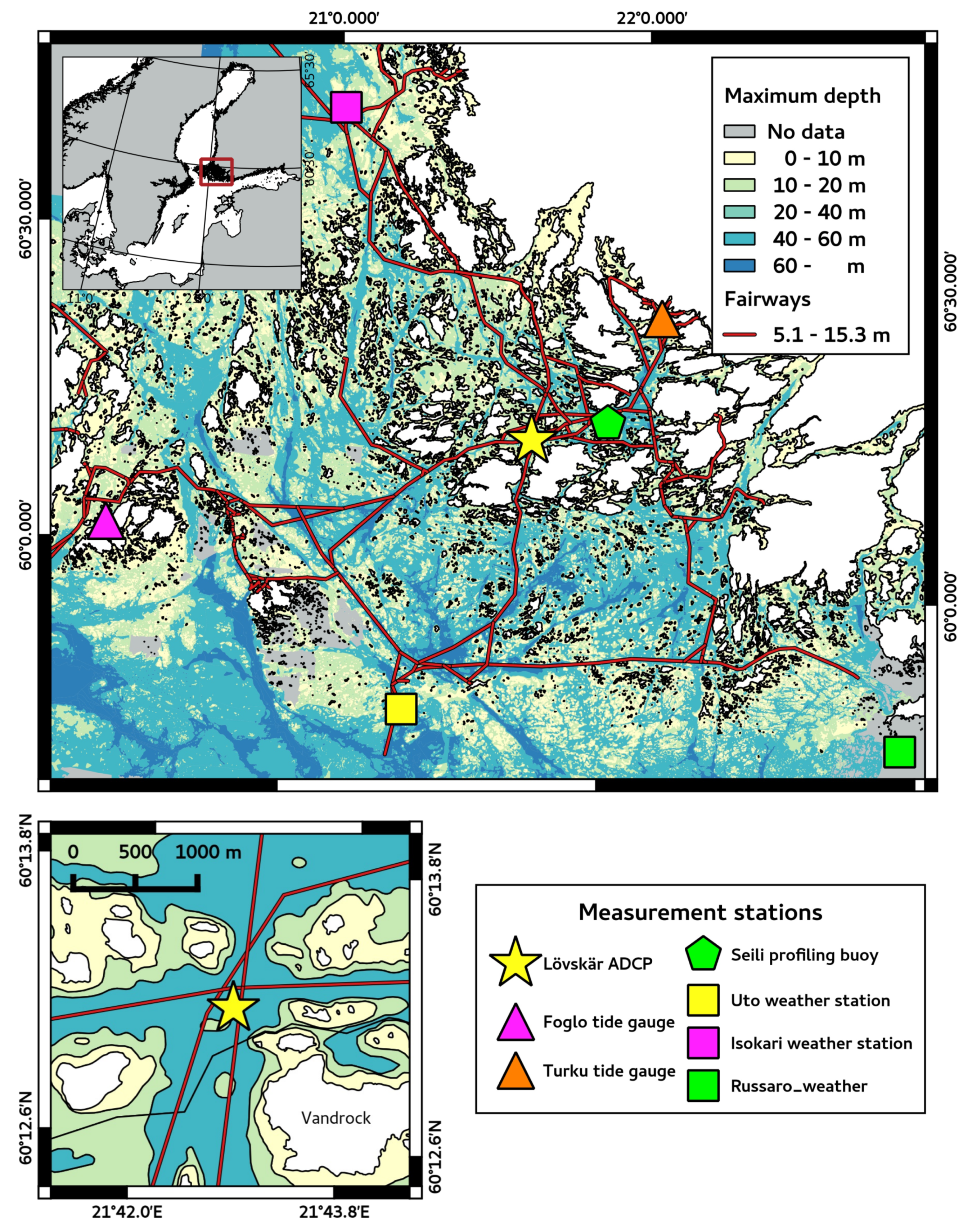
Current measurements were carried out in the Finnish Archipelago Sea near Lövskär Island (6013.183 N, 2142.800 E, Figure 1) between 18 June and 13 November 2013. Bathymetry of the measurement area—based on nautical charts from the Finnish Transport Agency—is shown in Figure 1. The site was chosen to be in a flat-bottom area that is also as deep as possible but under the fairways so that it measures the current conditions that the ships feel when passing by the basin. We expected that even big ships less affect the currents than natural forcing at that point, though the ships certainly have some effect on currents in the archipelago [23].
Current profiles were measured with bottom-mounted 300 kHz Workhorse Sentinel ADCP by Teledyne RD Instruments. The ADCP was bottom mounted in the centre of the cross section of two highly trafficked ship lanes (Figure 1). The measurement range was from about 5 m above the sea bed to 5 m below the surface, together 34 m. The depth cell (bin) size was 1 m and the measurement interval 20 min. Each velocity measurement is a weighted average of 120 pings around the midpoint of each depth cell.
2.2. Oceanographic Data
We used sea level and water temperature measurements from the routine observation stations in the Archipelago Sea to evaluate the connection between sea level and stratification in the area. The closest tide gauges are located by Turku (6025.8 N, 2206.0 E) and by Föglö Degerby (6001.8 N, 2022.8 E). Locations are shown in Figure 1. We used hourly values of sea level for the whole period in question.
2.3. Meteorological Data
We used measured wind speed and direction from FMI’s automatic weather stations (AWS) on Utö (59.78 N, 21.37 E), Isokari (60.72 N, 21.03 E) and Russarö (59.77 N, 22.95 E). Locations also shown in Figure 1. Wind data with 10-min intervals were used for the period from which the ADCP measurements were available. Also, a longer period (1961–2016) of wind measurements from Utö was used with three-hour intervals to evaluate the occurrence and directionality of strong wind events. Further information on this 56-year dataset reader is referred to in Laakso et al. [5].
3. Quality Control of ADCP Data
The quality control—henceforth QC—we used is mainly based on information about the measurement process recorded by the ADCP and the surrounding conditions it had when the averaged end product was given. ADCP performs an internal quality-control procedure, which includes checks of return signal correlation, false target rejection (e.g., fish) and homogeneity of the measurement area [25]. ADCP saves information of these internal checks, which we used in our QC procedures.
Scatterers—that enable the ADCP to receive a signal—can also cause different types of errors to the ADCP signals: (1) if there are no scatterers or there are too few of them, ADCP is unable to measure the current (2) if the scatterers move relative to the surrounding water, we get a false estimate of the water speed. ADCP can automatically detect large fast scatterers, such as fish, and discard these signals from the final current estimate. However, zooplankton movement can cause problems for data quality, especially around the strong density gradients, such as thermocline.
Typically, near-surface or near-bottom data need to be removed from the dataset due to the strong side lobe of the return signal from these layers. For our device, the contaminated area is at least 6% of the vertical measurement range as the transducer angle is 20°, which resulted in us having reliable data 5 m from the water surface downwards. The number of acceptable bins can vary due to sea level variation. In our case, sea level variations in the area were small compared to the bin size, so it did not affect the vertical measurement range.
Our main source of quality-control instructions were [26,27]. We used three quality flags according to SeaDataNet’s [28] recommendation: 1—good (values are confidently known to be valid), 3—unreliable (data quality can be questionable, but is not necessarily invalid) and 4—bad (data didn’t pass quality thresholds and shouldn’t be used without further analysis).
In the QC procedure, we used five different qualifiers: BIT (Built-In Test), Correlation, Echo intensity, PG (Percent Good) and Error velocity (Table 1). BIT represents the health of the measurement device and values different from zero are error codes. Correlation refers to correlation in the return signals that needs to be high enough in at least three beams for measurement to be reliable. Echo intensity is not a measure of quality as such, but it can be used to identify amount of scatterers in the sea and large jumps in echo intensity in time can indicate the presence of fish or other disturbances in the measurement dataset that internal QC was not able recognize [27]. Percent good values tell how many pings passed internal QC and were able to produce velocity solution. PG1 value gives the percentage of solutions made with three beams—meaning that one beam didn’t pass internal QC test—and PG4 percentage measured using all four beams [25]. Error velocity detects errors in measurement caused by inhomogeneity of the currents or malfunction in device [29]. Measurements made with 4 beams give two values of vertical motion and error velocity is the difference of these two values. Error velocity is high if one of the beams measures very different values from others. The threshold of this test is based on minimum accepted standard deviation (), which value depends on the bin size, device frequency and amount of pings averaged.
We used averaged echo intensity and flagged the data using error velocity only if PG4-value was over 10%. In addition, we used time and distance to the sea–air or sea–seabed interface to delimit data and checked the data for suspicious movements of the mooring. The minimum accepted standard deviation in our measurements was 12.4 mm/s. The threshold values for each qualifier were determined according to References [26,27] and are presented in Table 1. For further information of these qualifiers cf. [27].
The QC rejected 0.8% of the data. Most of these values were near to the thermocline depth, and as they occurred typically during dusk/night, we assume these to be related to zooplankton activity. In July and August, there were some events where ADCP measured very strong—around 0.3–0.4 ms—currents in few-metre layer above the thermocline. After some consideration, we marked these cases manually as probably bad (3), as they didn’t seem physically possible and because they occurred at the same time of the day as zooplankton activity was high. Most prominent occurrences of this behaviour happened on 7th July and between 20th–26th August. This extra precaution of the quality didn’t affect the uppermost layer—which is mainly studied in this paper. The total amount of rejected data was 1.4%.
In the subsequent analysis, we only use data with quality flag 1—good.
4. Results
4.1. Currents at Lövskär Crossing
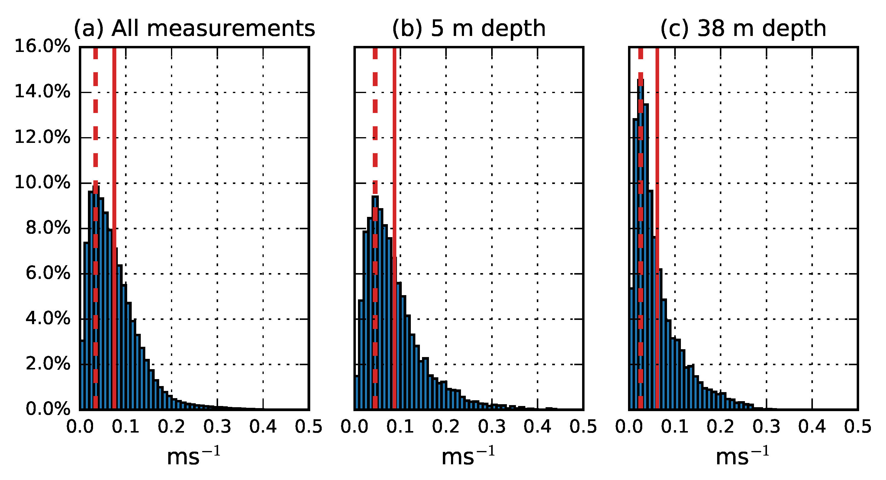
During the measurement period of 18th June to 13th November, 2013, the time and depth averaged measured current speed was 0.075 ms with a mode of 0.034 ms and standard deviation of 0.054 ms (Figure 2). Of the values, 74% were less than 0.10 ms and only 3% exceeded the magnitude of 0.20 ms. The current speeds were usually larger near the surface than near the bottom, as expected. However, there was not a large difference in the maximum values between the surface and bottom. In the near surface layer, at 5 m depth, the maximum measured value was 0.44 ms, and in the near bottom layer, 38 m depth, the value was 0.41 ms. As most of the measured current speeds were significantly smaller than 0.1 ms, occasional stronger currents, of over 0.2 ms, shifted the arithmetic mean of the current speed towards higher values (Figure 2). Because of this, we consider the mode to be a more descriptive value for overall conditions in the area.
The current directions were largely affected by the geometry and bathymetry of the area (Figure 1). There are four main directions from which the water masses can enter the measuring site: S, W, N and E straits. S and W straits are long wider straits, going between larger islands and connecting the cross section to more open sea areas of the Archipelago Sea and the Baltic Proper. N and E straits are surrounded by a large amount of different-sized islands, E strait being narrowest of these.
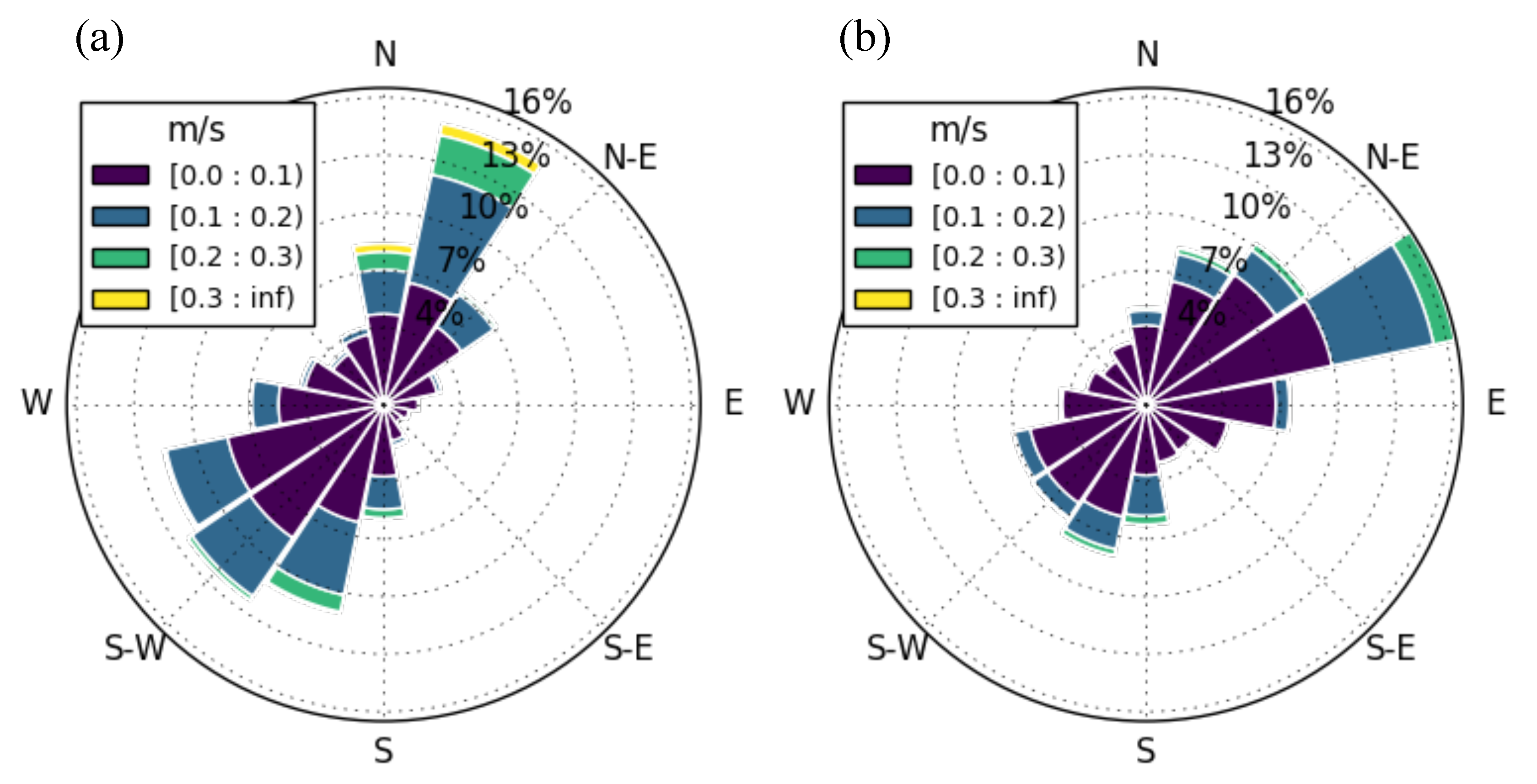
Current measurements showed that the currents had two main directions in the cross-section: NE and SW (Figure 3). In the surface layer (at 5 m depth), the prevailing direction was NNE with 14.7% of the cases (Figure 3a), whereas the prevailing direction near the bottom (at 38 m depth) was towards east-northeast (ENE) with 16.4% of the cases (Figure 3b).
4.1.1. Connection between Measured Winds and Near-Surface Currents
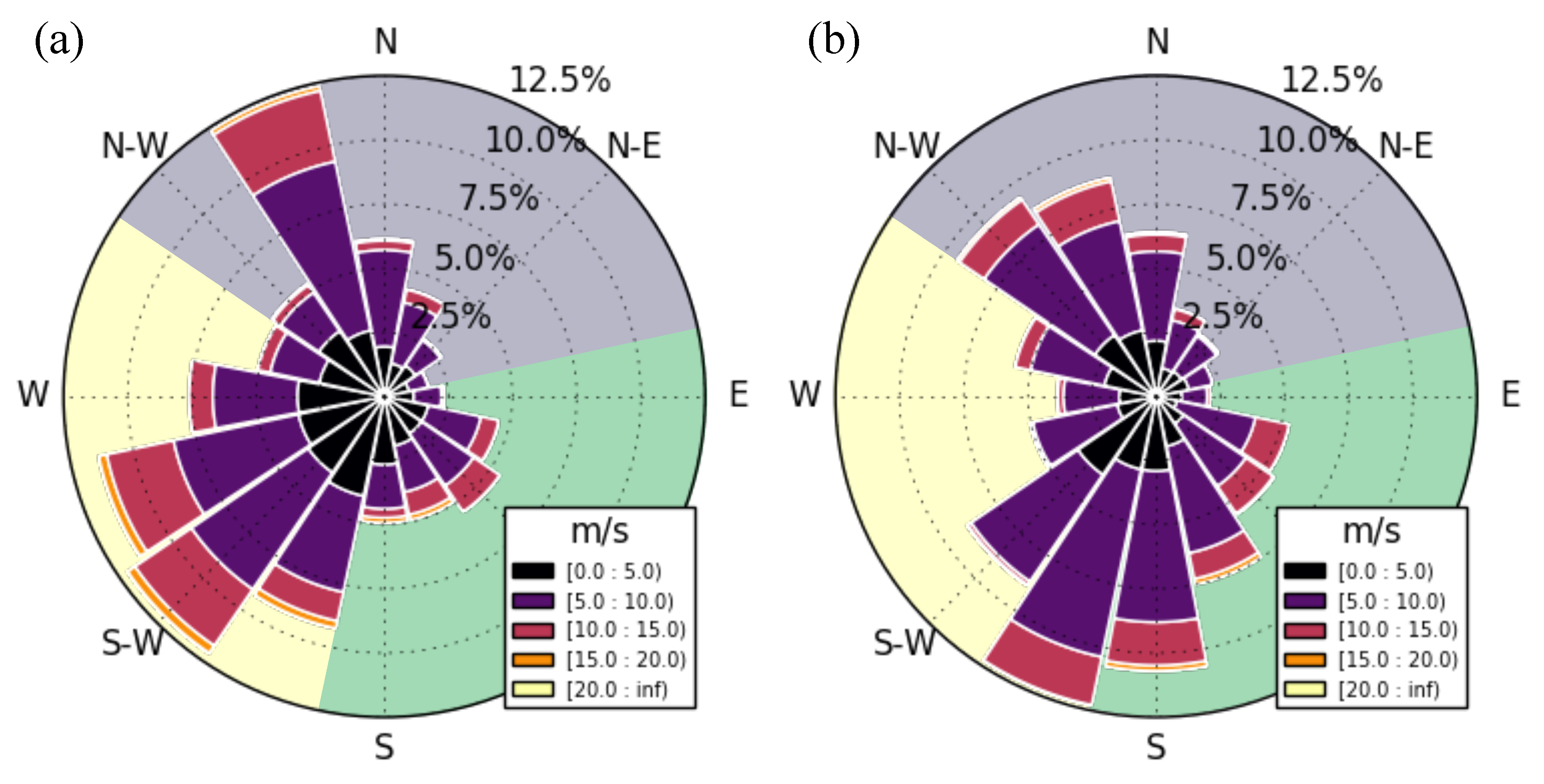
In order to study how the wind conditions induce and affect the currents, we studied in more detail the near-surface currents. We divided the dataset into three different sectors according to flow behaviour and the geometry of the measurement location. The goal was to have these sectors representing the main channels through which the wind induces currents into the cross section. Wind directions were first divided into 16 equal-sized sectors, centring the sectors to the main cardinal directions. From these sectors, we combined three sectors based on directional distribution of the currents and the shapes of outer areas of straits: 79–190, 191–303 and 304–78, which we henceforth call S, W and N respectively (Table 2, Figure 4). We did not separate E strait from N, as the surrounding conditions in these straits were similar. Both had a large amount of small islands and there was no clear geographical separation between them considering the surface currents. Moreover, only 11% of the winds measured at Utö station were from NNE and E (11°–100°) and only 0.8% of them had a speed of over 10 ms. Thus this definition did not have a significant effect on the results.
Of the currents, 45.6% were from westerly strait (Table 2) resulting from the prevailing wind direction that was from SW (Figure 4). The northern strait was the second most common with 32.1% of the currents coming from that direction. This is in good accordance with earlier studies about the wind conditions in the northern Baltic Proper (e.g., [31]), according to which SW and N are the most prominent wind directions in the Baltic Proper, while easterly winds are the least common.
The currents entering from the western strait are generally weaker than those from the S and N straits. The mean current speed from W sector was 0.077 ms and mode 0.035 ms, whereas the mean and mode of speed from N sector was 0.099 ms and 0.045 ms and from S 0.092 ms and 0.045 ms (Table 2, Figure 5d–f). As the W sector has the strongest winds overall (Figure 5g–i), this indicates that the westerly strait is not very optimal for winds to drive currents. The most likely reason behind this is the shape of the strait, that curves from a 225 angle by a more open archipelago to the 270 by the cross section (Figure 1). The turning of currents towards the right, due to the Coriolis force [32], makes this sector even more unfavourable for formation of strong currents with SW winds. The case is slightly opposite in the S strait, where the mode of the current speed is largest (0.057 ms Table 2). It is deeper and wider with fewer small islands restricting the flow (Figure 1). Also, the curve in the southern part of the strait allows water to enter the strait more easily. The current magnitude distribution is somewhat different with winds from the northern sector (Figure 5, current magnitude histogram on right) as it has fewer weaker currents, below 0.07 ms, but the amount of stronger, over 0.15 ms, currents is somewhat similar to the distribution of currents from S sector.
4.1.2. Seasonal Variability
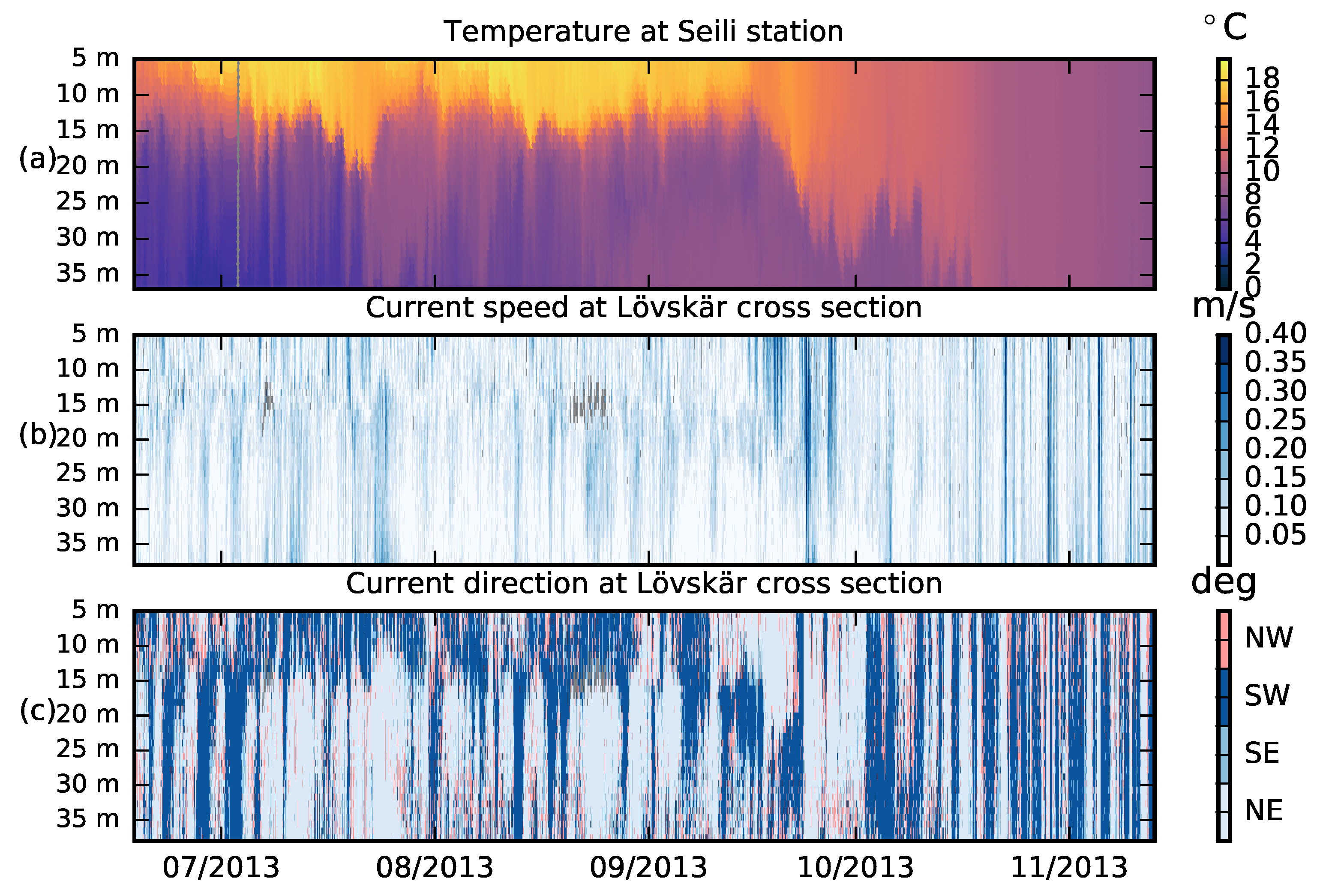
The measured currents showed strong vertical stratification from the beginning of the measurement period, 18th June until 23th September, which was the density stratified summer season (Figure 6). Interestingly, in the lower depths, the direction was often opposite to that of the upper layer (5–15 m). In the surface layer, the prevailing direction was towards SW; whereas, in the bottom layer, it was towards NE. The stratification is related to the seasonal thermocline, which limits the effect of wind stress to the upper mixed layer. The surface mixed layer breaks in autumn due to overturning induced by cooling and wind-induced mixing. Both temperature and current measurements showed the mixing and breaking of the vertical stratification between 24th September and 14th October. After the mixing, the wind-driven currents penetrated through the whole water column.
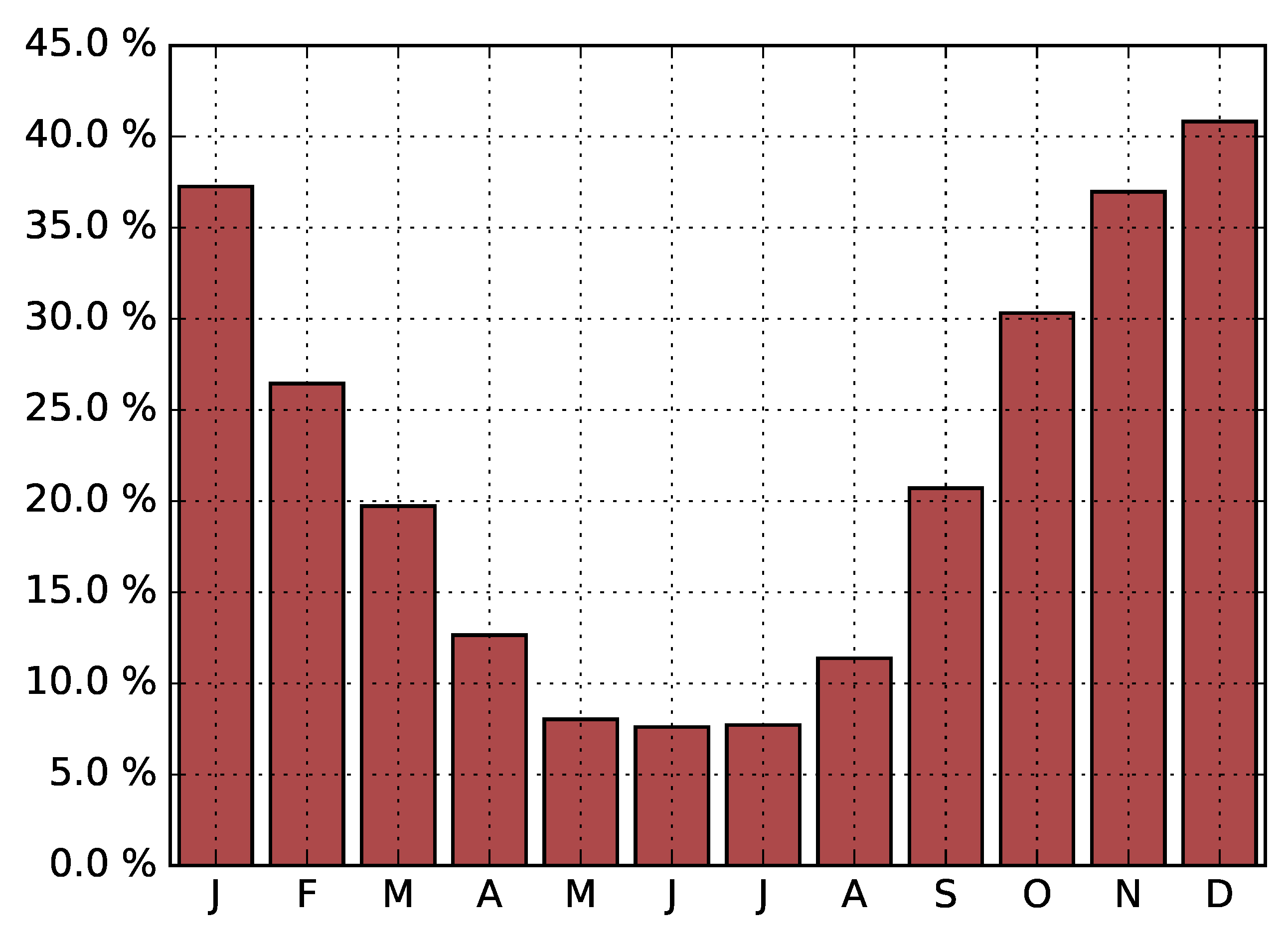
Generally, the current speeds are much stronger during autumn, than during the summer. This is due to the seasonality of the winds; during autumn and winter, the wind speeds are typically higher than during spring and summer (Figure 7).
4.2. Strong Current Events
To further evaluate the occurrence and frequency of strong currents, which may affect the marine traffic at the Lövskär crossing, we extracted events during which the current speed stayed consistently over 0.2 ms for at least 3 h for closer evaluation. In the whole measured water column, the current speed exceeded 0.2 ms about 3% of the time and in the surface-most 5 m layer about 6% of the time. In total, there were 22 events which fulfilled the criteria. Of these 22 events, four had surface current speed of over 0.4 ms (Table 3).
Average duration of all events reaching over 0.2 ms was 3.4 h, and for the more closely studied 22 events, this was about 7 h, ranging between 3–13.3 h. Four of these events occurred during the time the seasonal thermocline was present, and then the strong currents appeared only in the surface mixed layer. Moreover, the current speeds were generally weaker compared to the events in late summer and autumn. Of the 22 events, 11 occurred in September during the time when the seasonal overturning process started and was active. These cases were long-lasting, strong events (Figure 6, late September). During Autumn, after the overturning, there were seven events with strong currents. Compared to earlier events, the strong currents here were measured over the whole water column. These events varied from the weakest—18th October—with a maximum value of 0.27 ms to the strongest—22th October—with a maximum value of 0.44 ms.
As wind stress is the main driver of the surface currents in our study area, we evaluated the relationship between the strong current events at Lövskär (Figure 3) and the high wind events at Utö and at Isokari (Figure 4). Both of these weather stations are relatively far from the ADCP location (cf. Figure 1), but can be considered as representative for the overall wind conditions in this area. As the Utö AWS is located in the southern edge of the archipelago, it well represents the winds blowing from the open sea area south of the Archipelago Sea. On the other hand, Isokari AWS represents open sea conditions north of the archipelago. Furthermore, we used sea-level measurements at two tide gauges to evaluate the sea-level changes due to the strong current events. For a detailed description of the datasets, see Section 2.2.
4.2.1. Influence of Wind Direction to Currents
All of the 22 strong current events were induced by wind speed of over 10 ms but shorter lasting events occasionally formed with wind speed slightly over 5 ms. However, not all high wind events resulted in strong currents. Due to the narrowness and geometry of the channels, formation of strong currents is more sensitive to the wind direction than the wind speed.
Winds of over 10 ms occurred most often from W sector, with 54% of all winds over this magnitude blowing from there (Figure 4a). Considering the N sector, Utö had winds of over 10 ms mainly from NNW, but Isokari measurements showed that the Archipelago Sea experiences these winds both from NW and N (Figure 4b). Winds from S sector were the least common, but there were still many occasions when winds of over 10 ms were measured. The measurement period had only a few measurements of wind speed over 20 ms and all of them occurred in the autumn months after thermocline had eroded.
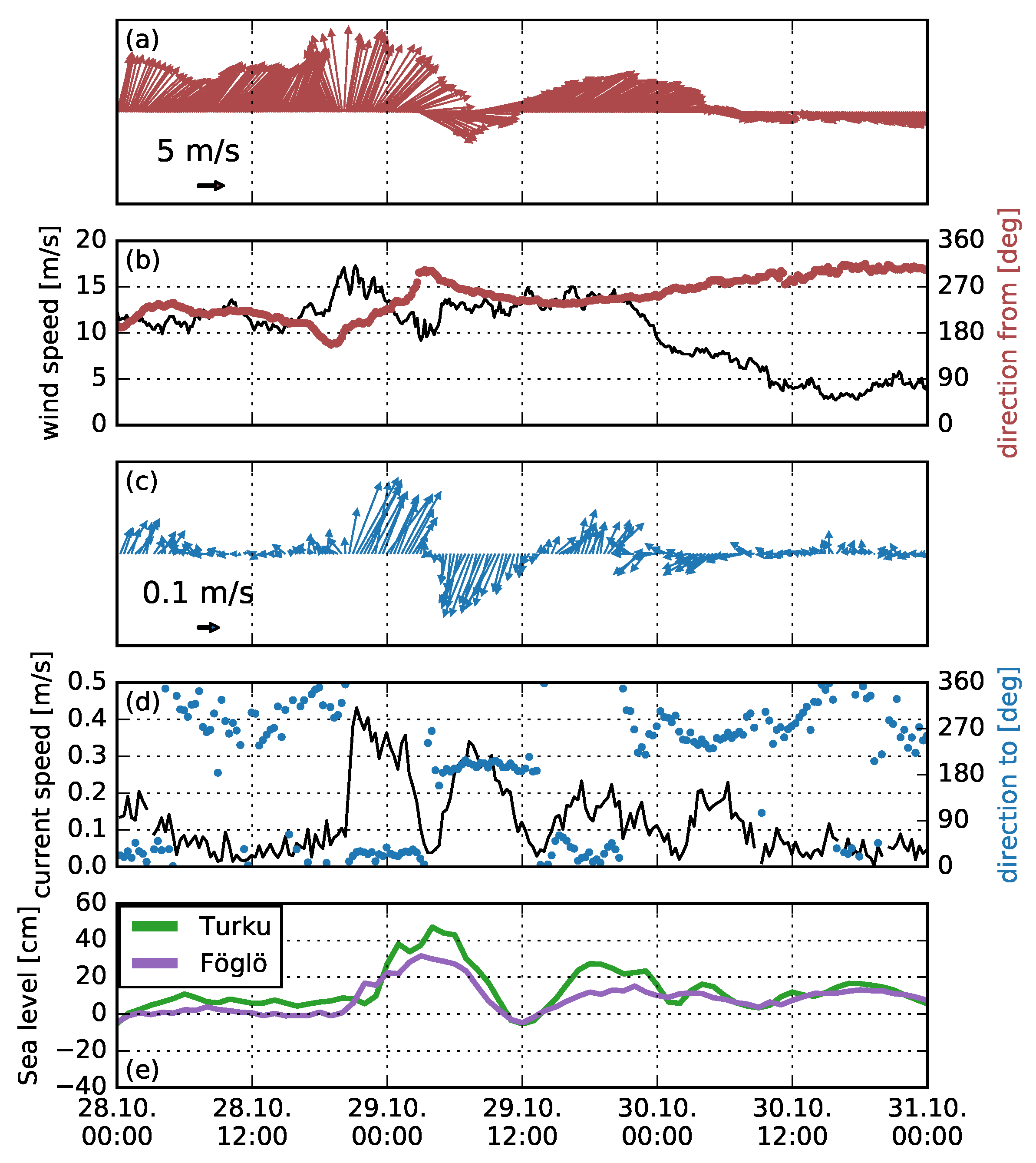
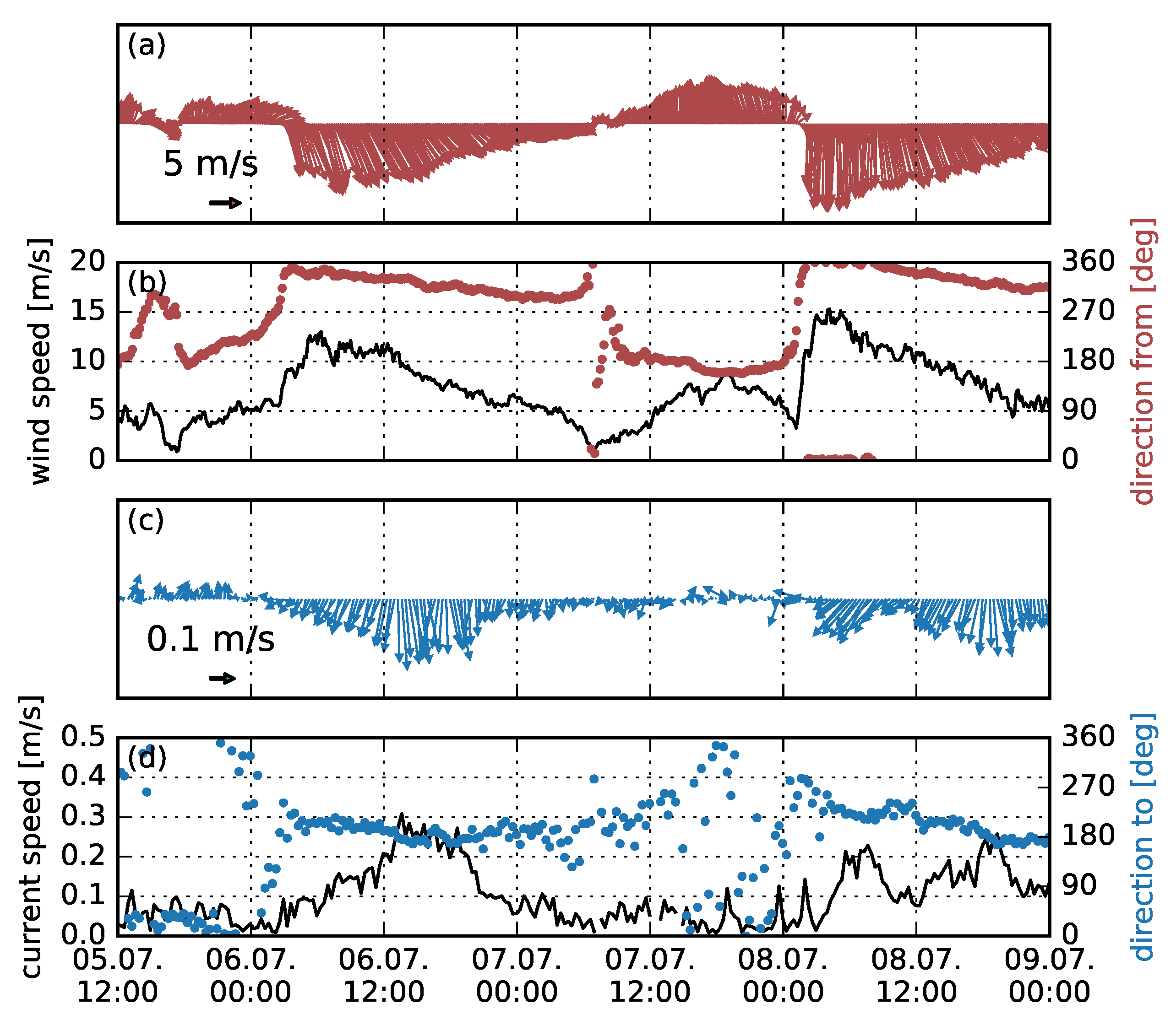
By studying the connection between the strong current events and Utö winds, we were able to conclude that the S strait is most open for direct influence of the strong winds. Three out of four cases, where current magnitude reached over 0.4 ms (Table 3), were along this strait. One of these strong current events occurred on 22 October (Figure 8), when the current speed rose as wind steadily grew while blowing from SSE. Measurements show that relatively small increase in wind speed and turning to favourable direction can induce a rapid increase in the currents’ speed, as was the case on 28 October (Figure 9). In this event, the sea level rise in Turku followed the wind and current peaks and the changes were small. Thus the sea level cannot be used as a proxy for high current speeds.
We used winds from the Isokari AWS to study connection between wind and current speed from the northerly sector. Based on these measurements, NNW is the most favourable direction for creating strong current events (Figure 10). From the northerly sector, the seasonal stratification had the most prominent effect on the magnitude of the surface currents. On 6th July, NW winds of a magnitude slightly over 10 ms induced a current event with a magnitude of 0.31 ms that lasted 6.3 h, whereas on 18th October, after the mixing of the water column, 15 ms N winds generated an event of 0.27 ms that lasted only 3 h. During the period, when the stratification exists, the momentum flux from the atmosphere is mainly received by the upper mixed layer, which is the most probable reason behind the differences of these two cases.
As SW winds were prevailing during our study period and had the most cases of wind speeds of over 10 ms, we expected to identify many cases of strong currents from this sector. However, as mentioned in Section 4.1, currents from winds from this sector were generally weaker than from N or S. Even a wind event in which over 10 ms wind speed lasted over a day, occasionally peaking to 15 ms induced currents of only 0.17 ms (not shown). It can also be noted that when wind speed turns to the W sector during a strong current event, the current speed reduced quite rapidly (Figure 8, on 22nd October).
Due to the small amount of high wind cases from the easterly sector, we were not able to determine the directional range of winds that would induce strong currents from this sector. However there was one occasion in which wind speed of over 10 ms from 135 was able to induce strong currents, whereas the same wind speed from 100 was not.
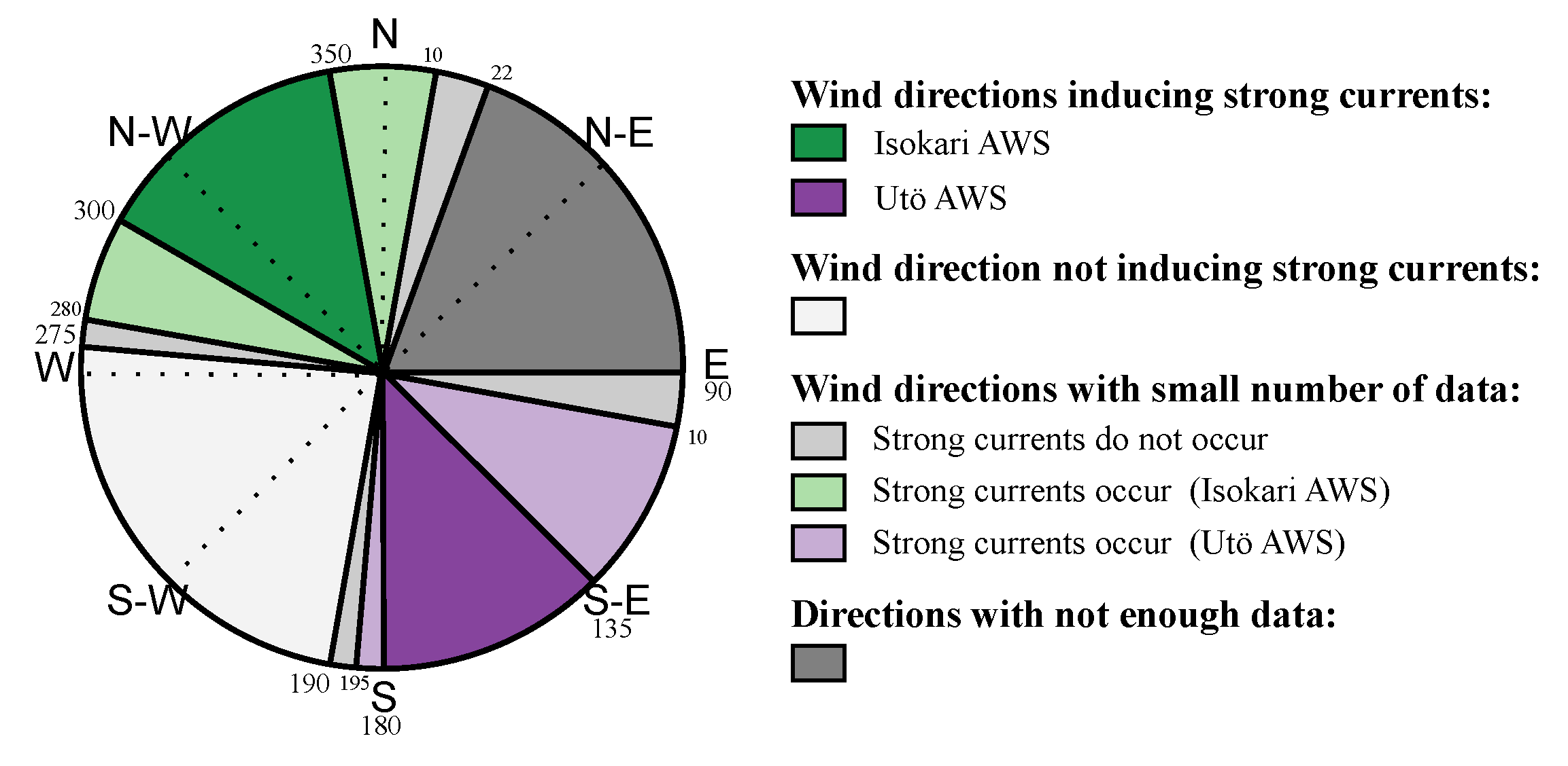
A summary of the directions that induce strong currents at the Lövskär crossing is presented in Figure 11.
4.2.2. Occurrence of Winds from Favourable DirectionsSubsubsection added
We studied the prevalence of the wind directions that induced strong currents using 56 years of measurements from Utö AWS. This is the period from which there are synoptic observations available at three-hour intervals. We chose Utö data for this analysis as it has longer temporal coverage than Isokari and has been earlier used in oceanographic studies by e.g., [5,22]. While contemplating the following results, one should note that Utö is not the most representative station for winds from the northerly sector, and the directional distribution measured there differs from actual winds experienced in northern parts of the Archipelago Sea. Therefore, the true relation of the SE and NW winds inducing the strong currents in the Lövskär crossing might slightly differ from the ones presented here.
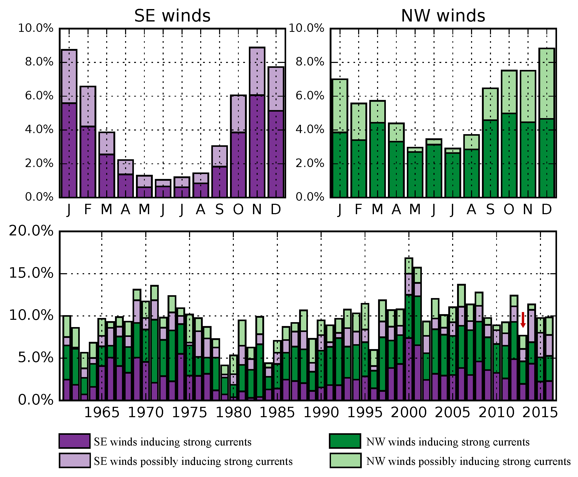
The long-term directional distribution of the winds was similar to our 5-month observation period (not shown). The prevailing directions were SW and NNW. However, the occurrence of easterly winds was more significant in the long-term time series than during our study period. The occurrence of winds of over 10 ms had some inter-annual variation (Figure 12, lower panel). Furthermore, occurrences of the SE winds have stronger seasonal variability than that of the NW winds (Figure 12, definition of the SE and NE sectors are given in Figure 11).
Winds of over 10 ms from the SE and NW occur annually on average 6.5% of the time from the directions we identified as winds that induce strong currents. The amount increases to 9.8% of the time if we include sectors that were identified as ones that probably induce strong currents. In our study year, 2013, the occurrence of SE and NW winds was rather low. Only 4.6% of the winds fulfilled the conditions of inducing strong currents (7.7%, if we include also probable directions). However, the seasonal distribution of these wind events was different from the average conditions (not shown), and our dataset included a large part of the events that occurred in 2013.
4.2.3. Return Currents Induced by Sea Level Change
The strong winds and currents induced sea level variation in the Archipelago Sea. Typically, the change in the sea level was of an order of a few tens of centimetres. Generally, northerly winds lowered and southerly winds raised the sea level in the Turku and Föglö stations (see locations in Figure 1). Winds of 15 ms caused the largest variations in sea level. During the strongest current events, which induced sea level changes of over 20 cm, the sea level reached maximum or minimum values typically 4–7 h after the wind and current speed maximum.
Two of the current events of over 0.4 ms induced the sea level to rise over 40 cm. One of these events was at the end of October (Figure 9) and the other at the beginning of November. In both of these cases, SE winds induced currents to a northerly direction, which was followed by a weaker current towards the opposite direction. Although the return currents were weaker than the main event inducing it, they both had values of over 0.3 ms. A similar event was seen on 9th November when the sea level rose over 40 cm. Then, the current speed rose to 0.35 ms and was followed by a counter current with a magnitude of 0.24 ms.
In all of these three cases, the return current peaked around half a day after initial event, and currents reached their minimum value around the same time as the sea level at Turku tide gauge peaked.
4.2.4. Discrepant Cases
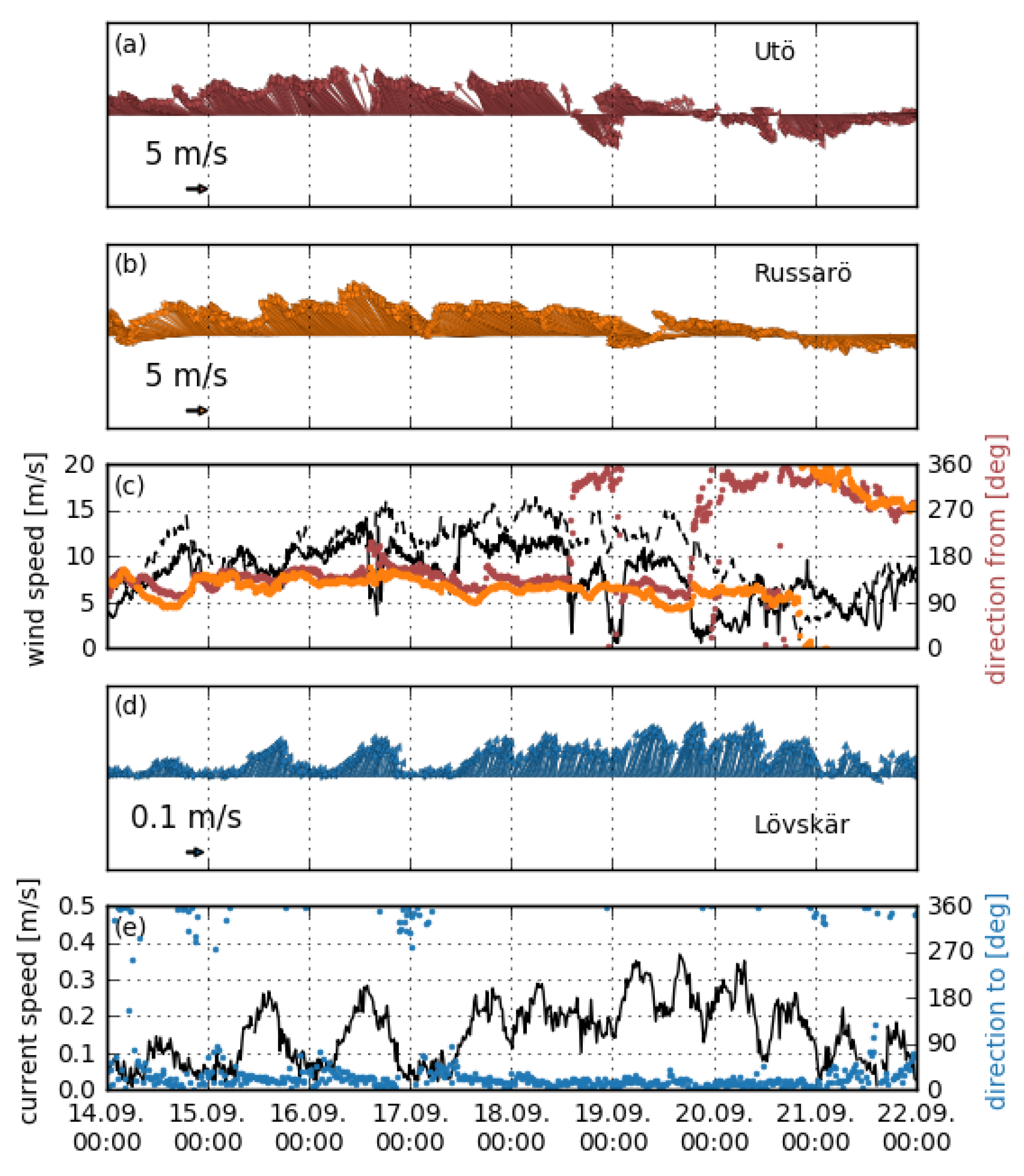
There were also a few strong current events that we were not able to directly connect to wind measurements at the Utö and Isokari stations. One such event was between 14th and 20th September, when there were strong northward currents up to 0.37 ms (Figure 13). For the first few days, the strong currents were clearly induced by winds that were also visible by the Utö measurements. At Utö, the wind speed mostly exceeded 10 ms for over 2.5 days, starting from 16th September. On the 18th, winds at the Utö station suddenly weakened and started to oscillate between NW and SE, finally settling to the NW. However, at the Russarö station, in the Gulf of Finland, located east of the study area (location shown in Figure 1), the wind speed was over 10 ms and even occasionally 15 ms from the ESE from 16th to 20th September. These ESE winds induced strong currents in the Finnish coast of the Gulf of Finland, which turned towards the Archipelago Sea, being the most probable cause of the strong currents at the Lövskär crossing.
Also, during the time when the seasonal overturning took place, there were strong currents from 23th to 28th September, that could not be entirely linked to strong winds. During these events, the vertical component of the current was occasionally significantly higher than on average.
4.2.5. Note about Comparison to Ship AIS Data
To study if we could identify, how the strong currents affect the marine traffic, we used AIS2 data from the Lövskär crossing. For detailed analysis, we selected the strong current event induced by SE winds on 22 October (Figure 8). The AIS data includes ship identification number, position, speed, course, heading and rate of turn data. We selected 6 ships that passed the Lövskär crossing along the 15.3 m deep Utö–Naantali fairway crossing the area (The fairway can be seen in Figure 1). All except one of the vessels were passenger ferries. In the analysis, we used AIS data from 2 × 2 nmi area centered in the location of the ADCP.
We evaluated ship drift using course over ground (COG) and heading (HDG) of the ship. Ships passing the cross section around 7 pm on 22nd October experienced a notable drift of 58 cm occurring at the same time as strong currents of 0.436 ms were measured at the Lövskär crossing. Although, the strong currents are the most probable cause of the ship drift in this case, one should keep in mind that there are also other things that might cause drift, such as strong wind. A more detailed study is needed to further analyse how marine traffic at the Lövskär crossing is affected by the strong currents.
5. Discussion
We have analysed the current measurements made at a crossing of two fairways in the Archipelago Sea. It is a place where the currents have been reported to affect ship navigation (personal communication with Finnish Transport Agency officials) and especially the ships going along the East-West fairway (cf. Figure 1) may feel strong currents (and wind) from the side. The data used in this study came from a specific measurement campaign that was intended to study strong currents in the crossing. To extend the analysis, we also used other routine observations, such as wind and sea-level data, to evaluate the conditions inducing strong current events. These routine observations are continuously available to the sea traffic control centre and can be used to identify strong current events that could have an effect on the safety of the marine traffic at the Lövskär crossing.
Our analysis showed that strong currents of over 0.2 ms regularly occur in the cross section. During our study period of five months, there were 22 strong current events during which the current stayed over 0.2 ms for at least 3 h. In most of these cases, we were able to connect with high wind events measured at Utö or Isokari AWS. However, we also noticed that, in some cases, it is not so trivial to straightforwardly link the strong currents with wind measurements and sea level measurements at nearby locations. As we saw from the case on the 16th to 20th August (in Section 4.2.4), the Utö and Isokari measurements we used to evaluate the connection between the strong winds and currents did not alone explain this situation. The event was most likely induced by a strong wind event ongoing in the Gulf of Finland, shown at Russarö AWS measurements. Therefore, more data is needed to thoroughly find the connection between the forcing winds and the currents in this area. Also, reanalysed current fields could be used to evaluate the overall circulation conditions in the area.
Even with all the complexity of the phenomena considered, it was possible to identify and link most of the strong current events to the measured wind speed and direction at Utö and Isokari. This enables us to forecast some of the strong current events based on wind measurements at the Utö station. As operational current forecasting in such a complex area requires horizontal resolution of a few hundred metres, the present operational systems—e.g., the CMEMS Baltic Sea physical analysis and forecasts system (marine.copernicus.eu, product BALTICSEA_ANALYSIS_FORECAST_PHY_003_006)—with a horizontal resolution of 1 nmi, are not able to resolve the currents in the narrow channels of the Archipelago Sea. Because of this, being able to use wind measurements to forecast strong current events might be beneficial for the safety of shipping in this area.
Our observation period of 5 months didn’t include a sufficient range of strong winds from all the directions and this limits the extension of our analysis. Easterly winds during our observation period were less common than on average and we were not able to conduct analysis from this range of winds at all. Scarceness of the observations from other directions also made it difficult to identify the directions from which wind direction changes from generating strong currents to the cross section and not generating them.
The wind measurements at Utö 1961–2016 showed that the occurrence of the winds of over 10 ms is more common in late autumn and winter, indicating that then strong current events could be occurring in the cross-section even more frequently than during our study period. We also showed that the generation of strong currents was quite sensitive for wind direction. The SE (135°–180°) and NW (300°–350°) sectors were identified as sectors that induce strong currents, when the wind speed from these sectors exceeds 10 ms for a sufficiently long time (at least 3 h). There was a great deal of inter-annual variation in the high wind speeds from this sector. During our study year, 2013, only 5% of winds fulfilled the criteria of possibly inducing strong currents in the cross section. This was a relatively low value, since the highest percentages were up to 12% e.g., in years 2000 and 2001.
We used AIS data to evaluate, whether we can see the effect of strong currents in the marine traffic passing the Lövskär crossing. The interpretation of the data requires more thorough analysis, as the drift is influenced by several factors, not only currents. However, we found that AIS data can be used to identify the events, when ships experience drift, which gives possibilities to study how often currents affect marine traffic in the crossing.
6. Conclusions
We studied strong currents in a fairway crossing in a coastal archipelago based on ADCP measurements to see whether occasional strong currents in the area could be predicted using existing routine observations. Our analysis showed that, due to the bathymetry and geometry of the crossing and the surrounding islands, there was a clear connection between the strong current events, of over 0.2 ms and measured winds at the two automatic weather stations in the southern and northern edge of the Archipelago Sea. Our analysis showed that the generation of strong current events was also very sensitive to the wind directions as there were only limited sectors from which high winds were able to induce strong currents in the crossing, namely the SE (135°–180°) and NE (300°–350°).
From these NE and SE sectors, even winds of slightly over 5 ms caused short events of currents of over 0.2 ms. However, long lasting, strong current events require winds of over 10 ms and all of the events having currents speeds of over 0.4 ms were connected to winds of over 15 ms. Interestingly, the SW winds (190°–275°), which prevail in this area and have the largest percentage of the winds over 10 ms, were not able to induce strong currents in the fairway crossing. Measurements showed that even 15 ms winds from SW did not induce currents of over 0.2 ms in the cross section.
Some of the strong current events were accompanied by a strong increase in the sea level. In these events, there was a return current some time after the wind forcing had stopped, which was around a quarter of magnitude smaller than the initial current. There were also a few cases in which we were not able to find a direct connection between the strong current events and wind measurements at Utö and Isokari. One of these events was induced by strong winds and currents in the northern part of the Gulf of Finland, and others were connected to the overturning of the water column and eroding of seasonal stratification. These type of cases are difficult to predict only by using measured data from the Archipelago Sea.
Author Contributions
P.A. and R.H. conceived and designed the measurement campaign. Quality control of the ADCP data and data analysis were done by H.K. with great help from M.L. and P.A. while analysing the results. Writing of the paper was conducted mainly by H.K. and L.T., with large participation on editing by P.A. and E.M. M.L. performed the analysis of AIS data, E.M. provided her expertise on the modelling of the Archipelago Sea and R.H. on the ADCP measurements.
Funding
This work has been partly funded by Merenkulun säätiö / Sjöfartsstiftelsen.
Acknowledgments
The map was produced using free and open source software QGIS (https://qgis.org/en/site/) and we thank Sakari Äärilä for helping with the usage. Bathymetric data and fairways were extracted from the Finnish Transport Agency’s open data service (https://julkinen.liikennevirasto.fi/oskari/), licensed under the Creative Commons 4.0 International (CC BY 4.0) licence (https://creativecommons.org/licenses/by/4.0/deed.fi) retrieved 17 August 2018. The coastline was obtained from the European Environment Agency’s service (https://www.eea.europa.eu/data-and-maps/data/eea-coastline-for-analysis-1/gis-data/europe-coastline-shapefile), retrieved 7 December 2017.
Conflicts of Interest
The authors declare no conflict of interest. The founding sponsors had no role in the design of the study; in the collection, analyses, or interpretation of data; in the writing of the manuscript, and in the decision to publish the results.
Abbreviations
The following abbreviations are used in this manuscript:
| ADCP | Acoustic Doppler Current Profiler |
| AIS | Automatic Identification System |
| AWS | Automatic Weather Station |
| BIT | Built-In Test |
| CMEMS | Copernicus Marine Environment Monitoring Service |
| E | East |
| ENE | East-North-East |
| ESE | East-South-East |
| FMI | Finnish Meteorological Institute |
| HF | High Frequency |
| MDPI | Multidisciplinary Digital Publishing Institute |
| N | North |
| NE | North-East |
| NNE | North-North-East |
| NW | North-West |
| NNW | North-North-West |
| QC | Quality Control |
| S | South |
| SE | South-East |
| SSE | South-South-East |
| SW | South-West |
| SSW | South-South-West |
| UTC | Universal Time Coordinated |
| W | West |
References
- Johansson, M.M. Sea Level Changes on the Finnish Coast and Their Relationship to Atmospheric Factors. Ph.D. Thesis, Finnish Meteorological Institute, Helsinki, Finland, 2014. [Google Scholar]
- Seinä, A.; Peltola, J. Jäätalven kestoaika ja kiintojään paksuustilastoja Suomen merialueilla 1961–1990—Duration of the ice season and statistics of fast ice thickness along the Finnish coast 1961–1990. Finn. Mar. Res. 1991, 258, 3–46. [Google Scholar]
- Breivik, Ø.; Sætra, Ø. Real time assimilation of HF radar currents into a coastal ocean model. J. Mar. Syst. 2001, 28, 161–182. [Google Scholar] [CrossRef]
- Axell, L.; Liu, Y. Application of 3-D ensemble variational data assimilation to a Baltic Sea reanalysis 1989–2013. Tellus A Dyn. Meteorol. Oceanogr. 2016, 68, 24220. [Google Scholar] [CrossRef]
- Laakso, L.; Mikkonen, S.; Drebs, A.; Karjalainen, A.; Pirinen, P.; Alenius, P. 100 years of atmospheric and marine observations at the Finnish Utö Island in the Baltic Sea. Ocean Sci. 2018, 14, 617–632. [Google Scholar] [CrossRef]
- Hietala, R.; Lundberg, P.; Nilsson, J.A. A note on the deep-water inflow to the Bothnian Sea. J. Mar. Syst. 2007, 1, 255–264. [Google Scholar] [CrossRef]
- Lilover, M.J.; Elken, J.; Suhhova, I.; Liblik, T. Observed flow variability along the thalweg, and on the coastal slopes of the Gulf of Finland, Baltic Sea. Estuar. Coast. Shelf Sci. 2017, 195, 23–33. [Google Scholar] [CrossRef]
- Suhhova, I.; Liblik, T.; Lilover, M.J.; Lips, U. A descriptive analysis of the linkage between the vertical stratification and current oscillations in the Gulf of Finland. Boreal Environ. Res. 2018, 23, 83–103. [Google Scholar]
- Dohan, K. Ocean surface currents from satellite data. J. Geophys. Res. Oceans 2017, 122, 2647–2651. [Google Scholar] [CrossRef] [Green Version]
- Gade, M.; Seppke, B.; Dreschler-Fischer, L. Mesoscale surface current fields in the Baltic Sea derived from multi-sensor satellite data. Int. J. Remote Sens. 2012, 33, 3122–3146. [Google Scholar] [CrossRef]
- Suchandt, S.; Andreas, L.; Runge, H. Analysis of ocean surface currents with TanDEM-X ATI: A case study in the Baltic Sea. In Proceedings of the 2014 IEEE International on Geoscience and Remote Sensing Symposium, Quebec City, QC, Canada, 13–18 July 2014. [Google Scholar] [CrossRef]
- Breaker, L.C.; Gemmill, W.H.; DeWitt, P.; Crosby, D.S. A curious relationship between the winds and currents at the western entrance of the Santa Barbara Channel. J. Geophys. Res. Oceans 2003, 108. [Google Scholar] [CrossRef] [Green Version]
- Cutroneo, L.; Ferretti, G.; Scafidi, D.; Ardizzone, G.D.; Vagge, G.; Capello, M. Current observations from a looking down vertical V-ADCP: Interaction with winds and tide? The case of Giglio Island (Tyrrhenian Sea, Italy). Oceanologia 2017, 59, 139–152. [Google Scholar] [CrossRef]
- Ghaffari, P.; Chegini, V. Acoustic Doppler Current Profiler observations in the southern Caspian Sea: Shelf Currents and flow field off Feridoonkenar Bay, Iran. Ocean Sci. 2010, 6, 737–748. [Google Scholar] [CrossRef]
- Roach, A.; Aagaard, K.; Pease, C.; Salo, S.; Weingartner, T.; Pavlov, V.; Kulakov, M. Direct measurements of transport and water properties through the Bering Strait. J. Geophys. Res. Oceans 1995, 100, 18443–18457. [Google Scholar] [CrossRef]
- Dufresne, C.; Duffa, C.; Rey, V. Wind-forced circulation model and water exchanges through the channel in the Bay of Toulon. Ocean Dyn. 2014, 64, 209–224. [Google Scholar] [CrossRef]
- De Serio, F.; Mossa, M. Assessment of hydrodynamics, biochemical parameters and eddy diffusivity in a semi-enclosed Ionian basin. Deep Sea Res. Part II Top. Stud. Oceanogr. 2016, 133, 176–185. [Google Scholar] [CrossRef]
- Malcangio, D.; Melena, A.; Damiani, L.; Mali, M.; Saponieri, A. Numerical study of water quality improvement in a port through a forced mixing system. WIT Trans. Ecol. Environ. 2017, 220, 69–80. [Google Scholar]
- Mali, M.; Malcangio, D.; Dell’Anna, M.M.; Damiani, L.; Mastrorilli, P. Influence of hydrodynamic features in the transport and fate of hazard contaminants within touristic ports. Case study: Torre a Mare (Italy). Heliyon 2018, 4, e00494. [Google Scholar] [CrossRef] [PubMed]
- Virtaustutkimuksen Neuvottelukunta. Saaristomeren Virtaustutkimus; Merenkulkuhallitus, Merikarttaosasto: Turku, Finland, 1979. (In Finnish) [Google Scholar]
- Ambjörn, C.; Gidhagen, L. Vatten- och materialtransporter mellan Bottniska viken och Östersjön RHO 19 (Water and material transports between the Gulf of Bothnia and the Baltic Proper). In SMHI Rapporter Hydrologi och Oceanografi; Sveriges Meteorologiska och Hydrologiska Institut: Norrköping, Sweden, 1979. [Google Scholar]
- Tuomi, L.; Miettunen, E.; Alenius, P.; Myrberg, K. Evaluating hydrography, circulation and transport in a coastal archipelago using a high-resolution 3D hydrodynamic model. J. Mar. Syst. 2018, 180, 24–36. [Google Scholar] [CrossRef]
- Stefan, H.G.; Riley, J. Mixing of a Stratified River by Barge Tows. Water Resour. Res. 1985, 21, 1085–1094. [Google Scholar] [CrossRef]
- Loisa, O.; Körber, J.H.; Laaksonlaita, J.; Kääriä, J. High-resolution monitoring of stratification patterns in the Archipelago Sea, Northern Baltic Sea, using an autonomous moored vertical profiling system. In Proceedings of the OCEANS 2017—Anchorage, Anchorage, AK, USA, 18–21 September 2017; pp. 1–6. [Google Scholar]
- RD Instruments. Workhorse Commands and Output Data Format; P/N 957-6156-00; RD Instruments Acoustic Doppler Solutions: San Diego, CA, USA, 2001. [Google Scholar]
- Symonds, D.R. QA/QC Parameters for Acoustic Doppler Current Profilers; Application Note; Teledyne RD Instruments A Teledyne Techologies Company: San Diego, CA, USA, 2006. [Google Scholar]
- Book, J.W.; Perkins, H.; Signell, R.P.; Wimbush, M. The Adriatic Circulation Experiment Winter 2002/2003 Mooring Data Report: A Case Study in ADCP Data Processing; NRL/MR/7330–07-8999; US Naval Research Laboratory: John C. Stennis Space Center, MS, USA, 2007. [Google Scholar]
- SeaDataNet. Data Quality Control Procedures, 6th Framework of EC DG Research, SeaDataNet, 2.0 ed. 2010. Version 2. Available online: https://www.seadatanet.org/Standards/Data-Quality-Control (accessed on 24 November 2016).
- RD Instruments. Acoustic Doppler Current Profiler Principles of Operation, A Practical Primer, P/N 957-6156-00; Teledyne RD Instruments A Teledyne Techologies Company: San Diego, CA, USA, 2011.
- Kanarik, H. ADCP Virtausmittausten Laaduntarkastusmenetelmien KehittäMinen ja Soveltaminen Saaristomerellä. Master’s Thesis, University of Helsinki, PL 3 (Fabianinkatu 33), Helsinki, Finland, 2018. [Google Scholar]
- Soomere, T. Anisotropy of wind and wave regimes in the Baltic Proper. J. Sea Res. 2003, 49, 305–316. [Google Scholar] [CrossRef]
- Ekman, V.W. On the influence of the earth’s rotation on ocean-currents. Arkiv för Matematik, Astronomi och Fysik 1905, 2, 1–53. [Google Scholar]
| 1. | minimum accepted standard deviation |
| 2. | AIS (Automatic Identification System) is VHF system for broadcasting the navigational data. |
Figure 1.
Map of the study area. The Lövskär cross section is presented in the lower left corner of the figure. Bathymetry and the locations of the fairways (deeper than 5 m) extracted from the Finnish Transport Agency’s open data base are shown. Areas in which bathymetric data were not available are presented with grey colour. The coast line is based on open-access data from the European Environment Agency.

Figure 2.
Current speed distribution over the whole water column (a), at the upper-most measured depth (b) and at the bottom-most measured depth (c). Solid red line represents arithmetic mean and dashed red line mode of the measurements.
Figure 2.
Current speed distribution over the whole water column (a), at the upper-most measured depth (b) and at the bottom-most measured depth (c). Solid red line represents arithmetic mean and dashed red line mode of the measurements.

Figure 3.
Current rose from measurements at 5 m depth (a) and at 38 m depth (b). Current direction is given as the direction where the flow is going to.
Figure 3.
Current rose from measurements at 5 m depth (a) and at 38 m depth (b). Current direction is given as the direction where the flow is going to.

Figure 4.
Wind roses from Utö (a) and Isokari (b) AWS June 18–November 13, 2013. Directions are given as the direction from where the wind is blowing. S (green), W (light yellow) and N (grey) sectors used in the study of strong current events are indicated on the background of the wind roses.
Figure 4.
Wind roses from Utö (a) and Isokari (b) AWS June 18–November 13, 2013. Directions are given as the direction from where the wind is blowing. S (green), W (light yellow) and N (grey) sectors used in the study of strong current events are indicated on the background of the wind roses.

Figure 5.
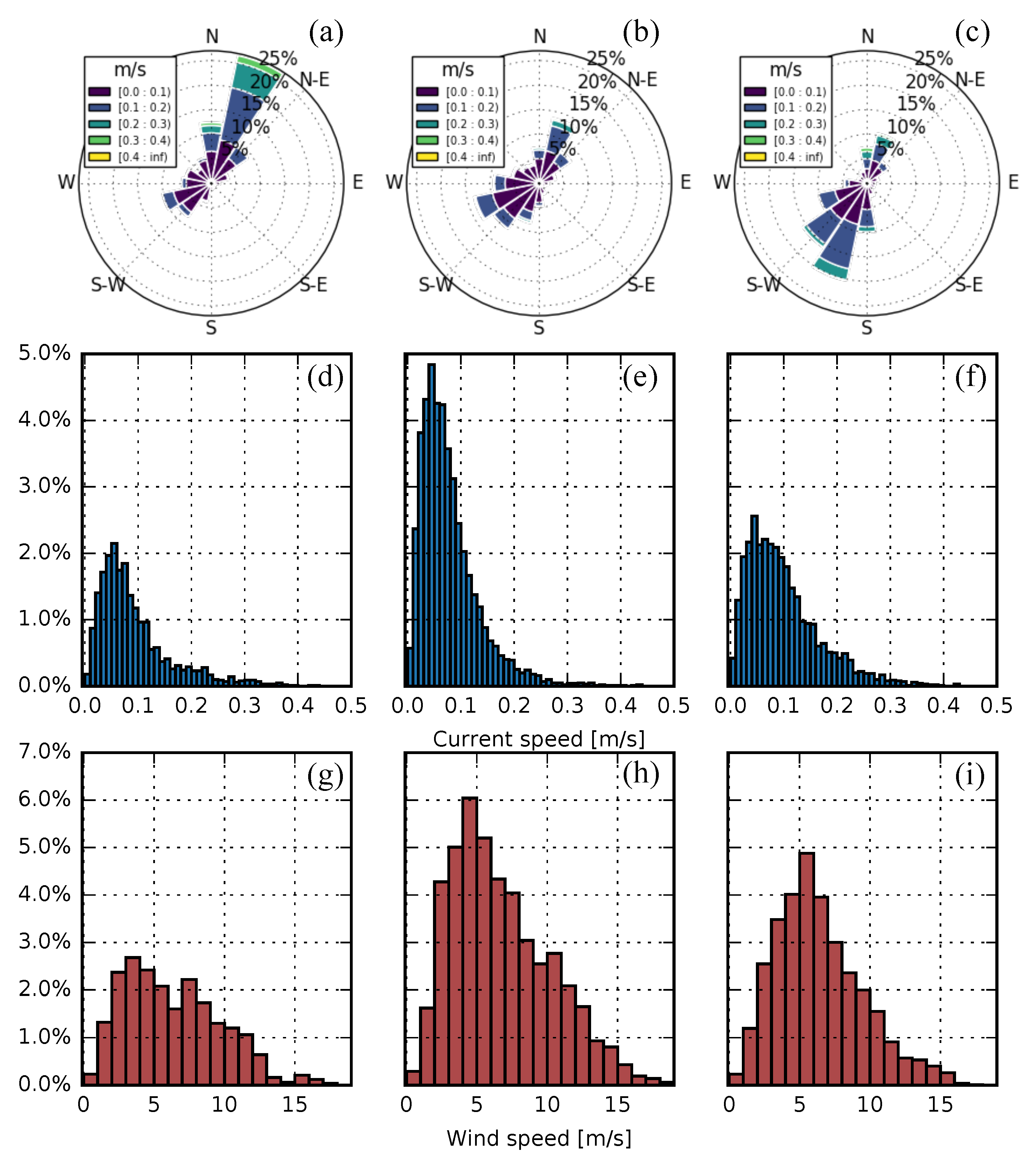
Current roses (a–c), histograms of the current speed (d–f) and histograms of the wind speed (g–i) for the S (left panels), W (middle panels) and N (right panels) sectors. Definition of sectors are shown in Figure 4. Percentages in the histograms represent the amount of currents and winds from a certain magnitude range from shown sector compared to the amount of measurements from the whole dataset. Only currents measured at 5 m depth are presented.
Figure 5.
Current roses (a–c), histograms of the current speed (d–f) and histograms of the wind speed (g–i) for the S (left panels), W (middle panels) and N (right panels) sectors. Definition of sectors are shown in Figure 4. Percentages in the histograms represent the amount of currents and winds from a certain magnitude range from shown sector compared to the amount of measurements from the whole dataset. Only currents measured at 5 m depth are presented.

Figure 6.
Temperature at Seili station (a), current magnitude (b) and the direction (c) at Lövskär cross section. Seili measurements have vertical coverage of 2–45 m, but only depths with the same range as current measurements are shown in this figure. Missing data points are shown as grey.
Figure 6.
Temperature at Seili station (a), current magnitude (b) and the direction (c) at Lövskär cross section. Seili measurements have vertical coverage of 2–45 m, but only depths with the same range as current measurements are shown in this figure. Missing data points are shown as grey.

Figure 7.
Percentage of winds of over 10 ms in each month. Based on Utö measurements from years 1961–2016.
Figure 7.
Percentage of winds of over 10 ms in each month. Based on Utö measurements from years 1961–2016.

Figure 8.
Wind speed and direction at Utö AWS (a,b) with current speed and direction at Lövskär crossing (c,d) during 21–24 October 2013. Locations of the measurement stations shown in Figure 1.
Figure 8.
Wind speed and direction at Utö AWS (a,b) with current speed and direction at Lövskär crossing (c,d) during 21–24 October 2013. Locations of the measurement stations shown in Figure 1.

Figure 9.
Wind speed and direction at Utö AWS (a,b), current speed and direction at Lövskär crossing (c,d) and sea level variation at Turku and Föglö tide gauges (e) 28–31 October 2013. Locations of the measurement stations shown in Figure 1.
Figure 9.
Wind speed and direction at Utö AWS (a,b), current speed and direction at Lövskär crossing (c,d) and sea level variation at Turku and Föglö tide gauges (e) 28–31 October 2013. Locations of the measurement stations shown in Figure 1.

Figure 10.
Wind speed and direction at Isokari AWS (a,b) with current speed and direction at Lövskär crossing (c,d) 5–9 July 2013. Locations of the measurement stations shown in Figure 1.
Figure 10.
Wind speed and direction at Isokari AWS (a,b) with current speed and direction at Lövskär crossing (c,d) 5–9 July 2013. Locations of the measurement stations shown in Figure 1.

Figure 11.
Wind directions distributed to the sectors according to their capability to induce strong currents at Lövskär crossing.
Figure 11.
Wind directions distributed to the sectors according to their capability to induce strong currents at Lövskär crossing.

Figure 12.
Monthly occurrences of winds over 10 ms from directions known to induce strong currents from years 1961–2016. Yearly occurrence of the favourable directions is shown in the bottom-most panel. Our study year of 2013 is pin pointed with a red arrow. Directions in question are visualised in Figure 11.

Figure 13.
Wind speed and direction at Utö and Russarö AWS (a–c), current speed and direction at Lövskär crossing (d,e) during 14–22 September 2013. In (c), magnitude of Utö winds is marked with solid line and Russarö winds with dashed line. Directions are marked with colours following the practice in upper panels. Locations of the measurement stations shown in Figure 1.


Table 1.
Threshold values used for ADCP (Acoustic Doppler Current Profiler) quality control.
| Parameter | Good Data (1) | Unreliable Data (3) | Bad Data (4) |
|---|---|---|---|
| BIT | 0 | ≠ 0 | — |
| Correlation | corr(of ≥3 beams) | corr(of 2 beams) | corr(of ≤1 beam) |
| Echo | No jump | jump >= 20 dB in time | — |
| Percent Good | PG1 + PG4 ≥ 60% | 60% > PG1 + PG4 > 35% | PG1+PG4 ≤ 35% |
| Error velocity | < | >1 and < | > |
Table 2.
Statistics of currents induced by winds from the S, W and N sectors. Gaps in wind and current data caused 0.8% of the data to be incomparable for this analysis.
Table 2.
Statistics of currents induced by winds from the S, W and N sectors. Gaps in wind and current data caused 0.8% of the data to be incomparable for this analysis.
| Current from | Wind from | Share | Max | Min | Mean | Mode |
|---|---|---|---|---|---|---|
| % | ms | ms | ms | ms | ||
| S sector | 79–190 (E–S) | 21.5 | 0.436 | 0.002 | 0.092 | 0.057 |
| W sector | 191–303(SSW–WNW) | 45.6 | 0.434 | 0.001 | 0.077 | 0.035 |
| N sector | 304–78(NW–ENE) | 32.1 | 0.427 | 0.002 | 0.099 | 0.045 |
Table 3.
Strongest measured current events, which exceeded 0.4 ms.
| Time [UTC] | Duration | Max Value [ms] |
|---|---|---|
| 2013/09/23 13:37–2013/09/23 23:57 | 9 h 20 min | 0.427 |
| 2013/10/22 14:37–2013/10/22 21:57 | 7 h 20 min | 0.436 |
| 2013/10/28 20:37–2013/10/29 02:17 | 5 h 40 min | 0.432 |
| 2013/11/05 03:37–2013/11/05 11:57 | 8 h 20 min | 0.434 |
© 2018 by the authors. Licensee MDPI, Basel, Switzerland. This article is an open access article distributed under the terms and conditions of the Creative Commons Attribution (CC BY) license (http://creativecommons.org/licenses/by/4.0/).
Share and Cite
MDPI and ACS Style
Kanarik, H.; Tuomi, L.; Alenius, P.; Lensu, M.; Miettunen, E.; Hietala, R. Evaluating Strong Currents at a Fairway in the Finnish Archipelago Sea. J. Mar. Sci. Eng. 2018, 6, 122. https://doi.org/10.3390/jmse6040122
AMA Style
Kanarik H, Tuomi L, Alenius P, Lensu M, Miettunen E, Hietala R. Evaluating Strong Currents at a Fairway in the Finnish Archipelago Sea. Journal of Marine Science and Engineering. 2018; 6(4):122. https://doi.org/10.3390/jmse6040122
Chicago/Turabian StyleKanarik, Hedi, Laura Tuomi, Pekka Alenius, Mikko Lensu, Elina Miettunen, and Riikka Hietala. 2018. "Evaluating Strong Currents at a Fairway in the Finnish Archipelago Sea" Journal of Marine Science and Engineering 6, no. 4: 122. https://doi.org/10.3390/jmse6040122
Note that from the first issue of 2016, this journal uses article numbers instead of page numbers. See further details here.