
Linking Coral Reef Remote Sensing and Field Ecology: It’s a Matter of Scale

Abstract
:
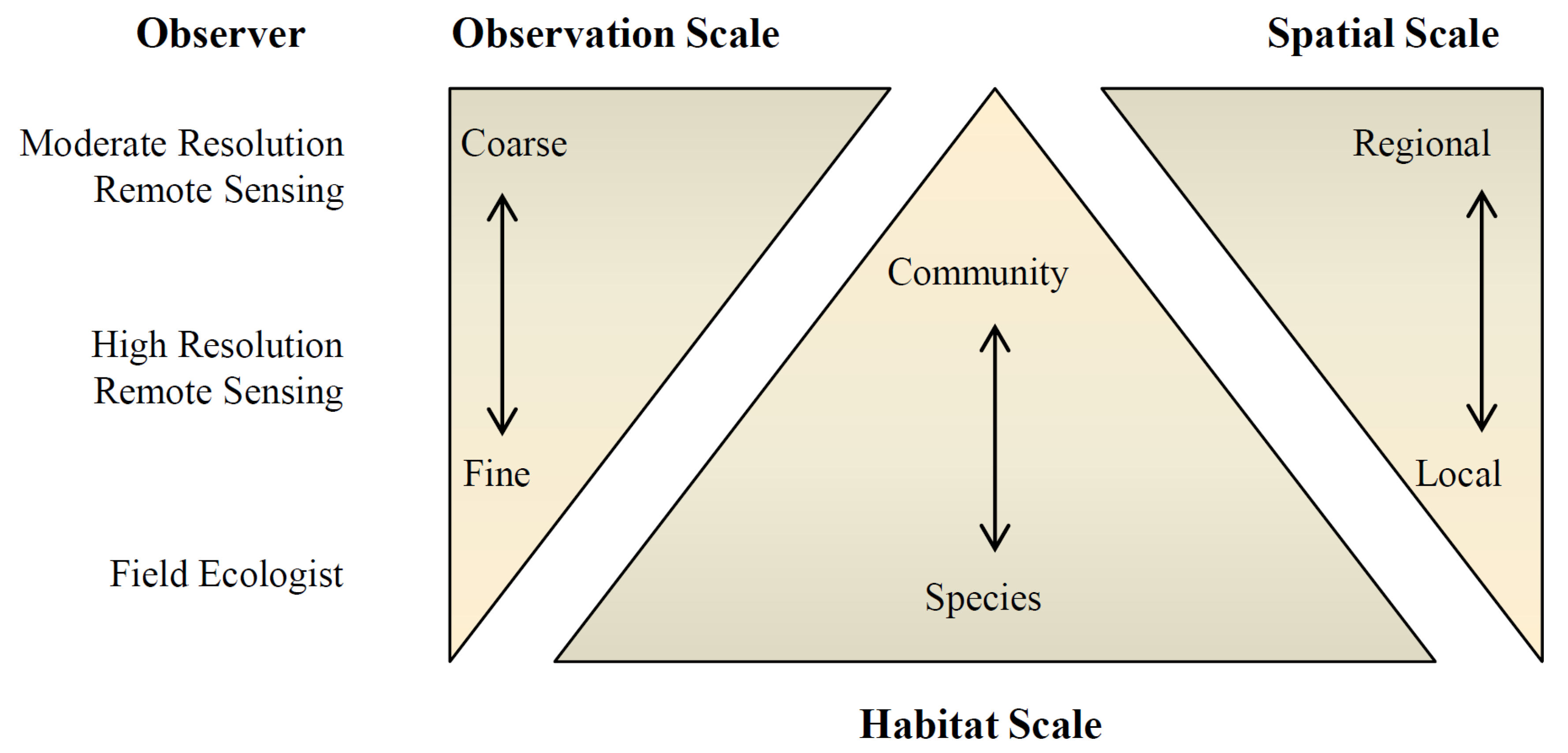
1. Introduction
2. Materials and Methods
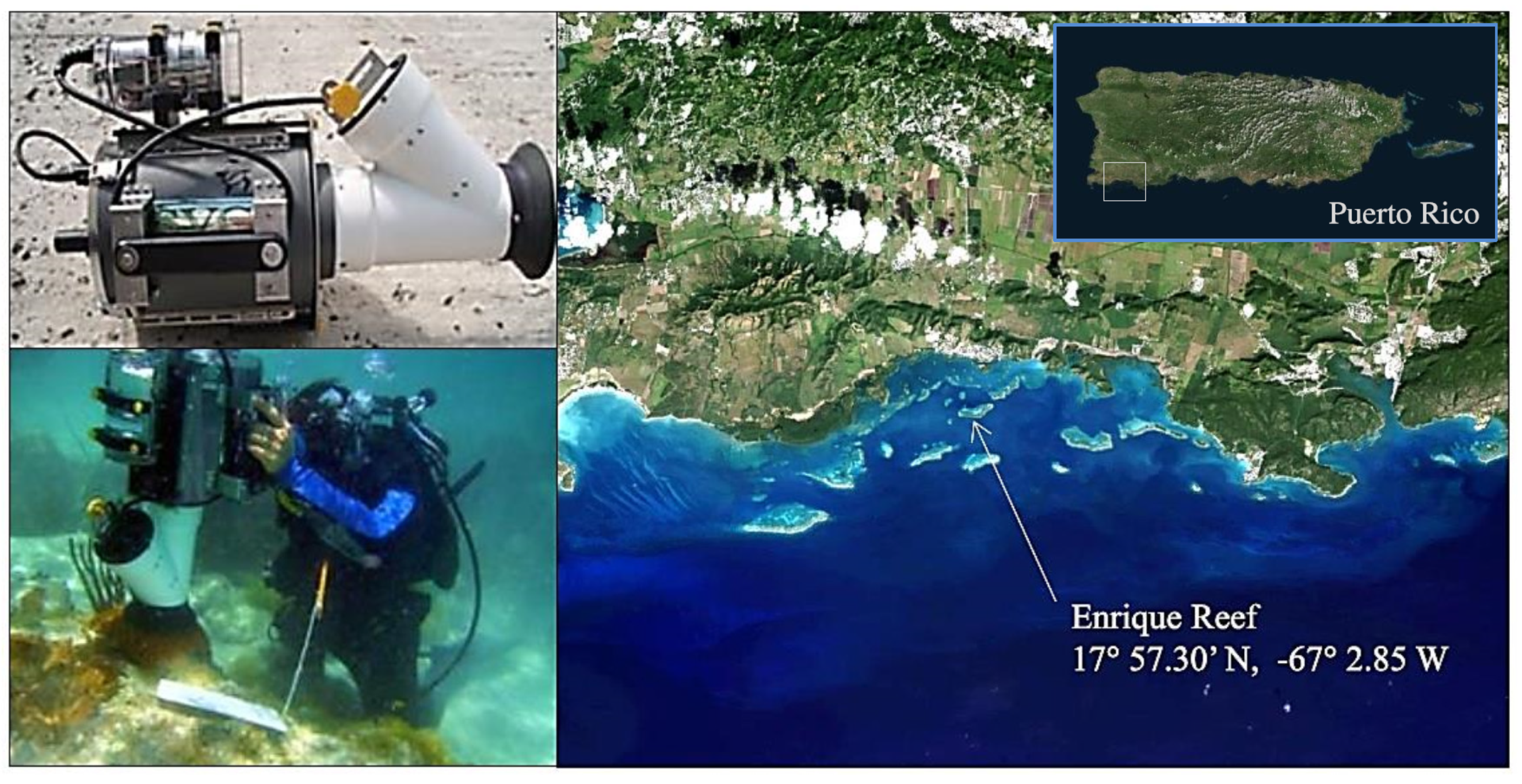
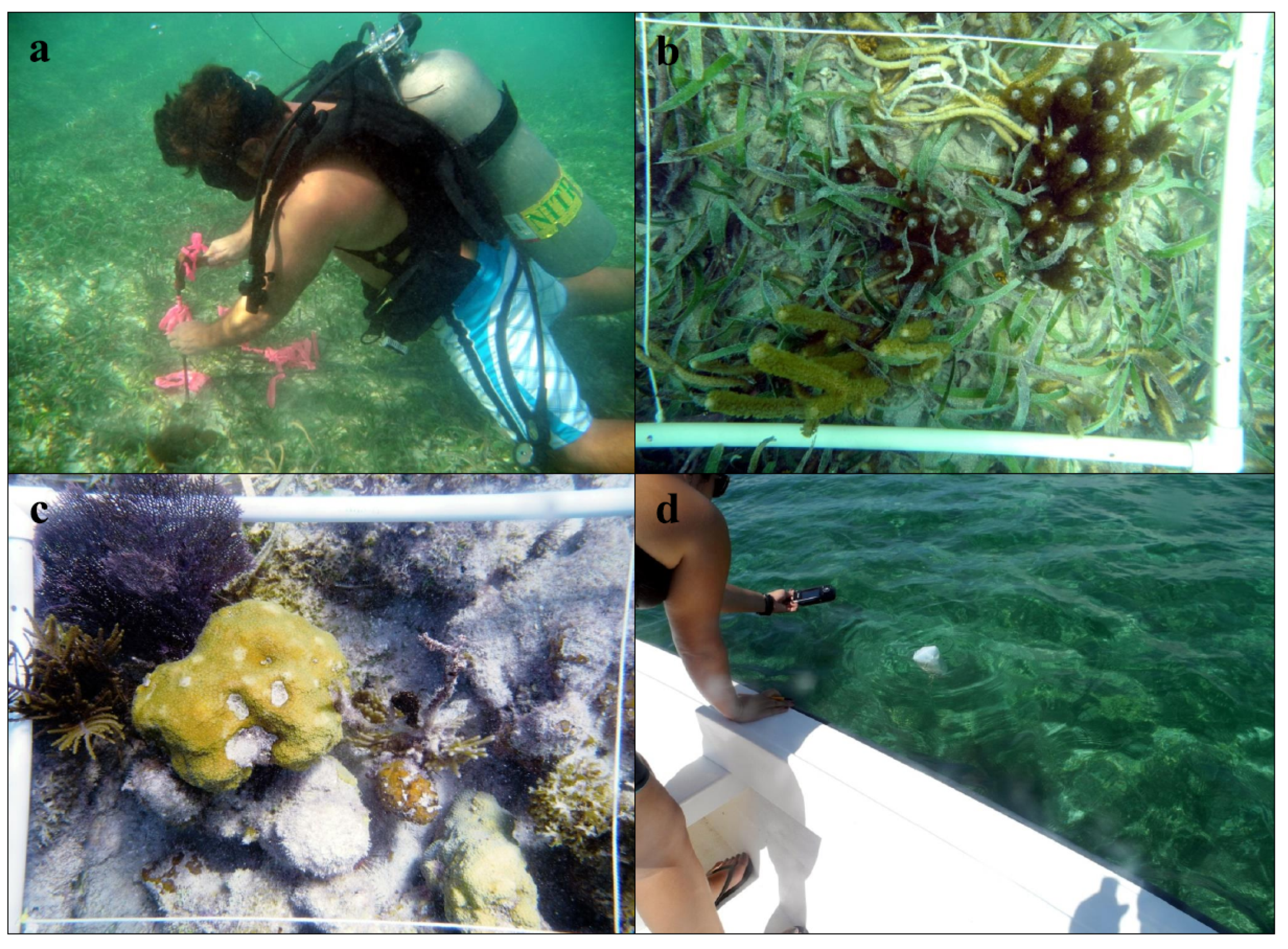
2.1. Reef Field Spectra

2.2. Separability Analysis and Water Column Modeling
2.3. Field Estimates of Biodiversity

3. Results
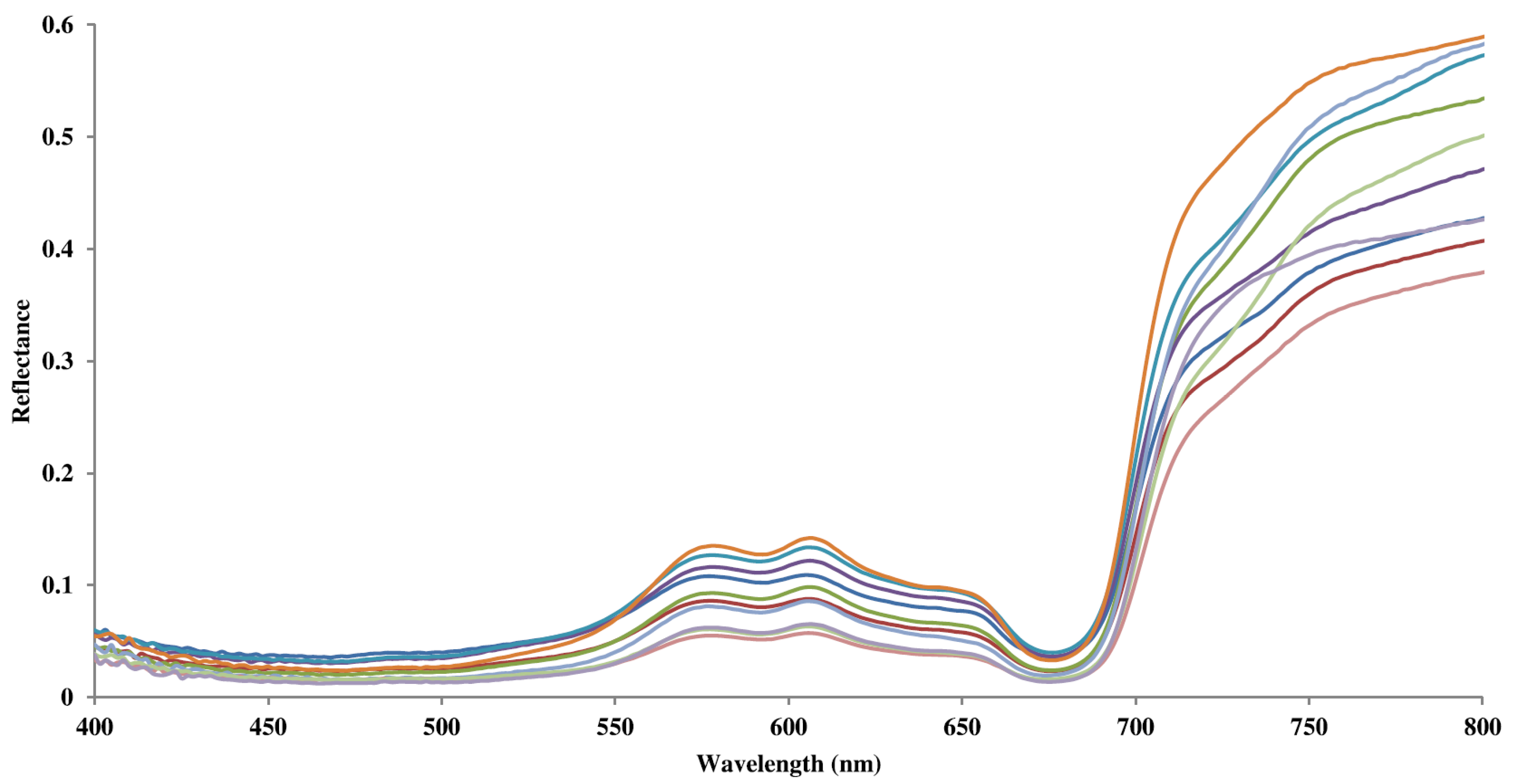
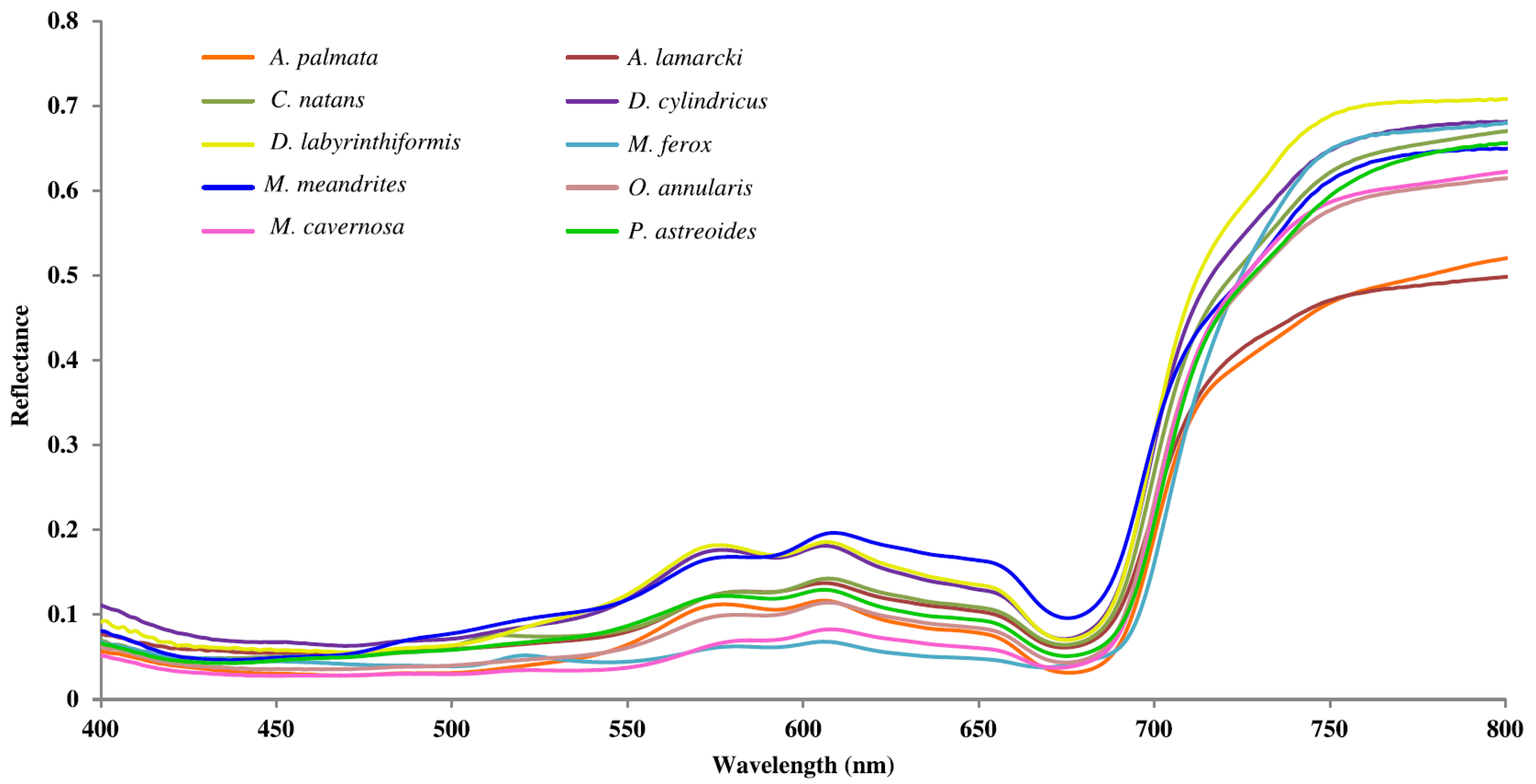
3.1. Reef Field Spectra

| Phylum | Individuals | Species/Type | Samples | Spectra R |
|---|---|---|---|---|
| Cnidaria | 73 | 25 | 5556 | 1389 |
| Porifera | 34 | 11 | 2028 | 507 |
| SAV (seagrass/algae) | Numerous | 4 | 1268 | 317 |
| Sand/Substrate | Numerous | 1 | 548 | 137 |
| Totals | 107 | 41 | 9400 | 2350 |


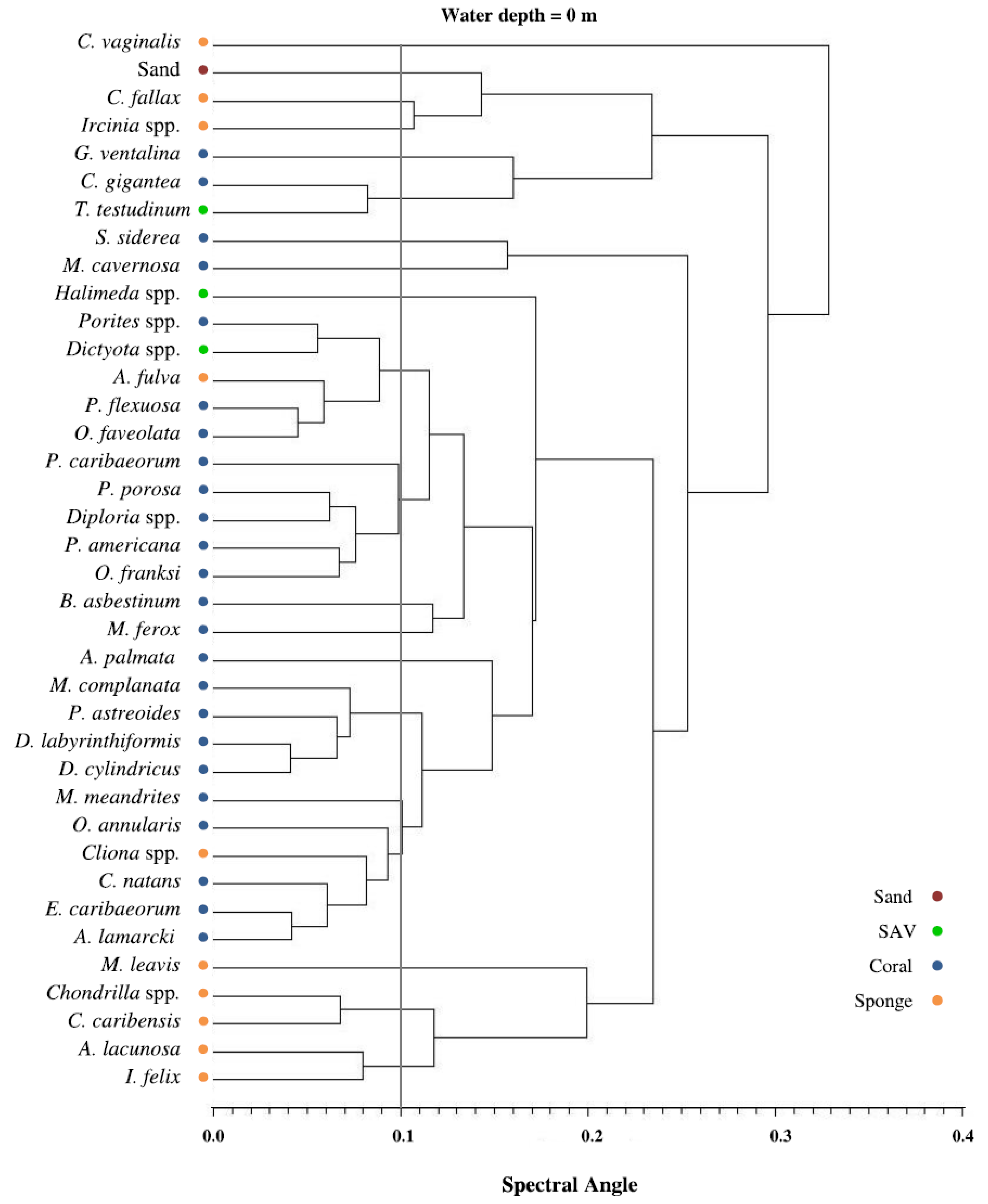
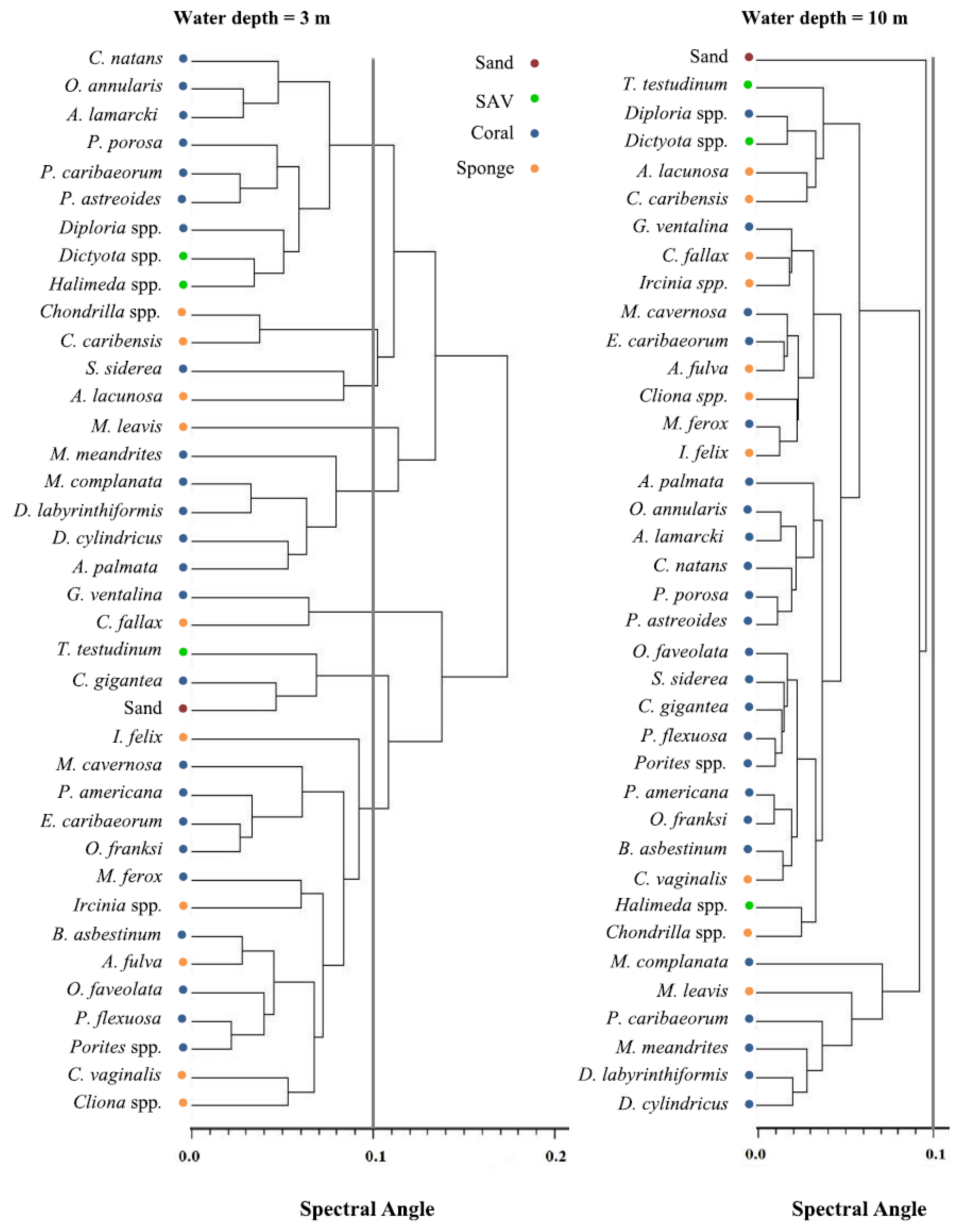
3.2. Spectral Separability


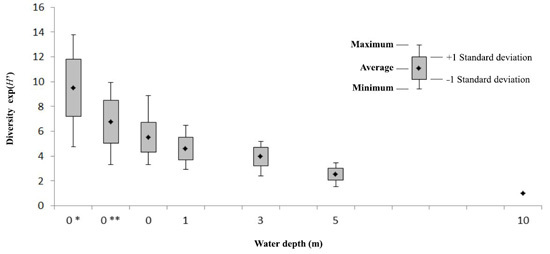
3.3. Field Estimates of Biodiversity

4. Discussion

5. Conclusions
Acknowledgments
Author Contributions
Conflicts of Interest
References
- Kerr, J.T.; Ostrovsky, M. From space to species: Ecological applications for remote sensing. Trends Ecol. Evol. 2003, 18, 299–305. [Google Scholar] [CrossRef]
- Turner, W.; Spector, S.; Gardiner, N.; Fladeland, M.; Sterling, E.; Steininger, M. Remote sensing for biodiversity science and conservation. Trends Ecol. Evol. 2003, 18, 306–314. [Google Scholar] [CrossRef]
- Wang, K.; Franklin, S.E.; Guo, X.; Cattet, M. Remote sensing of ecology, biodiversity and conservation: A review from the perspective of remote sensing specialists. Sensors 2010, 10, 9647–9667. [Google Scholar] [CrossRef] [PubMed]
- Walther, G.; Post, E.; Convey, P.; Menzel, A.; Parmesan, C.; Beebee, T.; Fromentin, J.; Hoegh-Guldberg, O.; Bairlein, F. Ecological responses to recent climate change. Nature 2002, 416, 389–395. [Google Scholar] [CrossRef] [PubMed]
- Hoegh-Guldberg, O.; Bruno, J.F. The impact of climate change on the world’s marine ecosystems. Science 2010, 328, 1523–1528. [Google Scholar] [CrossRef]
- Ateweberhan, M.; Feary, D.A.; Keshavmurthy, S.; Chen, A.; Schleyer, M.H.; Sheppard, C.R. Climate change impacts on coral reefs: Synergies with local effects, possibilities for acclimation, and management implications. Mar. Pollut. Bull. 2013, 74, 526–539. [Google Scholar] [CrossRef] [PubMed]
- Scopélitis, J.; Andréfouët, S.; Phinn, S.; Chabanet, P.; Naim, O.; Tourrand, C.; Done, T. Changes of coral communities over 35 years: Integrating in situ and remote-sensing data on Saint-Leu Reef (la Réunion, Indian Ocean). Estuar. Coast. Shelf Sci. 2009, 84, 342–352. [Google Scholar] [CrossRef]
- Scopélitis, J.; Andréfouët, S.; Phinn, S.; Arroyo, L.; Dalleau, M.; Cros, A.; Chabanet, P. The next step in shallow coral reef monitoring: Combining remote sensing and in situ approaches. Mar. Pollut. Bull. 2010, 60, 1956–1968. [Google Scholar] [CrossRef] [PubMed]
- Joyce, K.E. Spectral index development for mapping live coral cover. J. Appl. Remote Sens. 2013, 7, 073590. [Google Scholar] [CrossRef] [Green Version]
- Goodman, J.; Purkis, S.; Phinn, S. Coral Reef Remote Sensing: A Guide for Mapping, Monitoring, and Management; Goodman, J.A., Purkis, S.J., Phinn, S.R., Eds.; Springer Netherlands: Dordrecht, The Netherlands, 2013; pp. 1–436. [Google Scholar]
- Green, A. Designing a resilient network of marine protected areas in Kimbe Bay, West New Britain, Papua New Guinea. Oryx 2009, 43, 488–498. [Google Scholar] [CrossRef]
- Dalleau, M.; Andréfouët, S.; Wabnitz, C.C.; Payri, C.; Wantiez, L.; Pichon, M.; Friedman, K.; Vigliola, L.; Benzoni, F. Use of habitats as surrogates of biodiversity for efficient coral reef conservation planning in Pacific Ocean islands. Conserv. Biol. 2010, 24, 541–552. [Google Scholar] [CrossRef] [PubMed]
- Eakin, C.M.; Nim, C.; Brainard, R.; Aubrecht, C.; Elvidge, C.; Gledhill, D.; Muller-Karger, F.; Mumby, P.; Skirving, W.; Strong, A.; et al. Monitoring coral reefs from space. Oceanography 2010, 23, 118–133. [Google Scholar] [CrossRef]
- Medina, O.; Manian, V.; Chinea, J.D. Biodiversity assessment using hierarchical agglomerative clustering and spectral unmixing over hyperspectral images. Sensors 2013, 13, 13949–13959. [Google Scholar] [CrossRef] [PubMed]
- Mumby, P.J.; Skirving, W.; Strong, A.E.; Hardy, J.T.; Ledrew, E.F.; Hochberg, E.J.; Stumpf, R.P.; David, L.T. Remote sensing of coral reefs and their physical environment. Mar. Pollut. Bull. 2004, 48, 219–228. [Google Scholar] [CrossRef] [PubMed]
- Hochberg, E.; Atkinson, M. Capabilities of remote sensors to classify coral, algae, and sand as pure and mixed spectra. Remote Sens. Environ. 2003, 85, 174–189. [Google Scholar] [CrossRef]
- Lucas, R.; Mitchell, A.; Bunting, P. Hyperspectral remote sensing of tropical and subtropical forests. In Hyperspectral Remote Sensing for Assessing Carbon Dynamics and Biodiversity of Forests; Margaret Kalacska, G., Sanchez-Azofeifa, A., Eds.; CRC Press: London, UK, 2008; pp. 47–86. [Google Scholar]
- Goodman, J.; Ustin, S. Classification of benthic composition in a coral reef environment using spectral unmixing. J. Appl. Remote Sens. 2007, 1, 011501. [Google Scholar] [CrossRef]
- Lesser, M.P.; Mobley, C.D. Bathymetry, water optical properties, and benthic classification of coral reefs using hyperspectral remote sensing imagery. Coral Reefs 2007, 26, 819–829. [Google Scholar] [CrossRef]
- Herkül, K.; Kotta, J.; Kutser, T.; Vahtmäe, E. Relating remotely sensed optical variability to marine benthic biodiversity. PLoS One 2013, 8, e55624. [Google Scholar] [CrossRef] [PubMed]
- Joyce, K.; Phinn, S.; Roelfsema, C. Live coral cover index testing and application with hyperspectral airborne image data. Remote Sens. 2013, 5, 6116–6137. [Google Scholar] [CrossRef]
- Hochberg, E.J.; Atkinson, M.J.; Apprill, A.; Andréfouët, S. Spectral reflectance of coral. Coral Reefs 2004, 23, 84–95. [Google Scholar] [CrossRef]
- Karpouzli, E.; Malthus, T.J.; Place, C.J. Hyperspectral discrimination of coral reef benthic communities in the western Caribbean. Coral Reefs 2004, 23, 141–151. [Google Scholar] [CrossRef]
- Hedley, J.D.; Mumby, P.J.; Joyce, K.E.; Phinn, S.R. Spectral unmixing of coral reef benthos under ideal conditions. Coral Reefs 2004, 23, 60–73. [Google Scholar] [CrossRef]
- Hedley, J.D.; Roelfsema, C.M.; Phinn, S.R.; Mumby, P.J. Environmental and sensor limitations in optical remote sensing of coral reefs: Implications for monitoring and sensor design. Remote Sens. 2012, 4, 271–302. [Google Scholar] [CrossRef]
- Hochberg, E.; Atkinson, M.; Andréfouët, S. Spectral reflectance of coral reef bottom-types worldwide and implications for coral reef remote sensing. Remote Sens. Environ. 2003, 85, 159–173. [Google Scholar] [CrossRef]
- Hedley, J.D.; Mumby, P.J. Biological and remote sensing perspectives of pigmentation in coral reef organisms. Adv. Mar. Biol. 2002, 43, 277–317. [Google Scholar] [PubMed]
- Hedley, J. A three-dimensional radiative transfer model for shallow water environments. Opt. Express 2008, 16, 21887–21902. [Google Scholar] [CrossRef] [PubMed]
- Hedley, J.; Roelfsema, C.; Phinn, S.R. Efficient radiative transfer model inversion for remote sensing applications. Remote Sens. Environ. 2009, 113, 2527–2532. [Google Scholar] [CrossRef]
- Botha, E.J.; Brando, V.E.; Anstee, J.M.; Dekker, A.G.; Sagar, S. Increased spectral resolution enhances coral detection under varying water conditions. Remote Sens. Environ. 2013, 131, 247–261. [Google Scholar] [CrossRef]
- Pettorelli, N.; Safi, K.; Turner, W. Satellite remote sensing, biodiversity research and conservation of the future. Philos. Trans. R. Soc. Lond. B Biol. Sci. 2014, 369, 20130190. [Google Scholar] [CrossRef] [PubMed]
- Lubin, D.; Li, W.; Dustan, P.; Mazel, C.H.; Stamnes, K. Spectral signatures of coral reefs: Features from space. Remote Sens. Environ. 2001, 137, 127–137. [Google Scholar] [CrossRef]
- Knudby, A.; Jupiter, S.; Roelfsema, C.; Lyons, M.; Phinn, S. Mapping coral reef resilience indicators using field and remotely sensed data. Remote Sens. 2013, 5, 1311–1334. [Google Scholar] [CrossRef]
- Knudby, A.; LeDrew, E.; Newman, C. Progress in the use of remote sensing for coral reef biodiversity studies. Prog. Phys. Geogr. 2007, 31, 421–434. [Google Scholar] [CrossRef]
- Ziskin, D. Describing coral reef bleaching using very high spatial resolution satellite imagery: Experimental methodology. J. Appl. Remote Sens. 2011, 5, 053531. [Google Scholar] [CrossRef]
- Hedley, J.; Roelfsema, C.; Koetz, B.; Phinn, S. Capability of the Sentinel 2 mission for tropical coral reef mapping and coral bleaching detection. Remote Sens. Environ. 2012, 120, 145–155. [Google Scholar] [CrossRef]
- Holden, H. Accuracy assessment of hyperspectral classification of coral reef features. Geocarto Int. 2000, 15, 7–14. [Google Scholar] [CrossRef]
- Yamano, H.; Tamura, M. Detection limits of coral reef bleaching by satellite remote sensing: Simulation and data analysis. Remote Sens. Environ. 2004, 90, 86–103. [Google Scholar] [CrossRef]
- Anderson, D.A.; Armstrong, R.A.; Weil, E. Hyperspectral sensing of disease stress in the Caribbean reef-building coral, Orbicella faveolata—Perspectives for the field of coral disease monitoring. PLoS One 2013, 8, e81478. [Google Scholar] [CrossRef] [PubMed]
- Wiens, J. Spatial scaling in ecology. Funct. Ecol. 1989, 3, 385–397. [Google Scholar] [CrossRef]
- Marceau, D.J. The scale issue in social and natural sciences. 1999, 25, 347–356. [Google Scholar]
- Blaschke, T.; Geoffrey, J. Obect-oriented image analysis and scale-space: Theory, methods, and evaluating multiscale lanscape structure. Int. Arch. Photogramm. Remote Sens. 2001, 34, 22–29. [Google Scholar]
- Roelfsema, C.M.; Phinn, S.; Jupiter, S.; Comley, J.; Beger, M.; Patterson, E. The application of object based analysis of high spatial resolution imagery for mapping large coral reef systems in the west pacific at geomorphic and benthic community spatial scales. In Proceedings of the IEEE International Ultrasonics Symposium (IUS), San Diego, CA, USA, 11–14 October 2010; pp. 4346–4349.
- Goodman, J. Hyperspectral Remote Sensing of Coral Reefs: Deriving Bathymetry, Aquatic Optical Properties and a Benthic Spectral Unmixing Classification Using AVIRIS Data in the Hawaiian Islands. Ph.D. Dissertation, University of California, Davis, Davis, CA, USA, 2004. [Google Scholar]
- Goodman, J. 2007 Puerto Rico Hyperspectral Mission: Image Acquisition and Field Data Collection; University of Puerto Rico: San Juan, PR, USA, 2008; p. 56. [Google Scholar]
- Rueda, C.; Wrona, A. SAMS Spectral Analysis & Management System Users Manual; University of California, Davis: Davis, CA, USA, 2003. [Google Scholar]
- Lee, Z.; Carder, K.L.; Mobley, C.D.; Steward, R.G.; Patch, J.S. Hyperspectral remote sensing for shallow waters. I. A semi-analytical model. Appl. Opt. 1998, 37, 6329–6338. [Google Scholar] [CrossRef] [PubMed]
- Lee, Z.; Carder, K.L.; Mobley, C.D.; Steward, R.G.; Patch, J.S. Hyperspectral remote sensing for shallow waters. 2. Deriving bottom depths and water properties by optimization. Appl. Opt. 1999, 38, 3831–3843. [Google Scholar] [CrossRef] [PubMed]
- Kruse, F.A.; Lefkoff, A.B.; Boardman, J.W.; Heidebrecht, K.B.; Shapiro, A.T.; Barloon, P.J.; Goetz, A.F. The spectral image processing system (SIPS)-interactive visualization and imaging spectrometer data. Remote Sens. Environ. 1993, 44, 145–163. [Google Scholar] [CrossRef]
- Exelis Visual Information Solutions. Interactive Data Language 8.3 Reference Guide. Available online: http://www.exelisvis.com/docs/using_idl_home.html (accessed on 14 October 2014).
- Goodman, J.A.; Vélez-Reyes, M.; Rosario-Torres, S. An update on SeaBED: A TestBED for validating subsurface aquatic hyperspectral remote sensing algorithms. SPIE Remote Sens. 2008, 2. [Google Scholar] [CrossRef]
- Dethier, M.; Graham, E.; Cohen, S.; Tear, L. Visual versus random-point percent cover estimations: “Objective is not always better”. Mar. Ecol. Prog. Ser. 1993, 96, 93–100. [Google Scholar] [CrossRef]
- Pante, E.; Dustan, P. Getting to the point: Accuracy of point count in monitoring ecosystem change. J. Mar. Biol. 2012, 2012, 1–7. [Google Scholar] [CrossRef]
- Whittaker, R. Evolution and measurement of species diversity. Taxon 1972, 22, 213–251. [Google Scholar] [CrossRef]
- Jost, L. Partitioning diversity into independent alpha and beta components. Ecology 2007, 88, 2427–2439. [Google Scholar] [CrossRef] [PubMed]
- Hochberg, E.J.; Apprill, A.M.; Atkinson, M.J.; Bidigare, R.R. Bio-optical modeling of photosynthetic pigments in corals. Coral Reefs 2006, 25, 99–109. [Google Scholar] [CrossRef]
- Torres-Pérez, J.; Guild, L.; Armstrong, R. Hyperspectral distinction of two Caribbean shallow-water corals based on their pigments and corresponding reflectance. Remote Sens. 2012, 4, 3813–3832. [Google Scholar] [CrossRef]
- Segura, J. Water depth effects in photosynthetic pigment content of the benthic algae Dictyota dichotoma and Udotea petiolata. Aquat. Bot. 1981, 11, 373–378. [Google Scholar] [CrossRef]
- Roelfsema, C.M.; Phinn, S.R.; Udy, N.; Maxwell, P. An integrated field and remote sensing approach for mapping Seagrass cover, Moreton Bay, Australia. J. Spat. Sci. 2009, 54, 45–62. [Google Scholar] [CrossRef]
- Fuller, R.M.; Groom, G.B.; Mugisha, S.; Ipulet, P.; Pomeroy, D.; Katende, A.; Bailey, R.; Ogutu-ohwayo, R. The intergration of field survey and remote sensing for biodiversity assessement: A case study in the tropical forests and wetlands of Sango Bay, Uganda. Biol. Conserv. 1998, 86, 379–391. [Google Scholar] [CrossRef]
- Andréfouët, S.; Muller-Karger, Mumby, J.; McField, M.; Hu, C. Revisiting coral reef connectivity. Coral Reefs 2002, 21, 43–48. [Google Scholar] [CrossRef]
© 2014 by the authors; licensee MDPI, Basel, Switzerland. This article is an open access article distributed under the terms and conditions of the Creative Commons Attribution license ( http://creativecommons.org/licenses/by/4.0/).
Share and Cite
Lucas, M.Q.; Goodman, J. Linking Coral Reef Remote Sensing and Field Ecology: It’s a Matter of Scale. J. Mar. Sci. Eng. 2015, 3, 1-20. https://doi.org/10.3390/jmse3010001
Lucas MQ, Goodman J. Linking Coral Reef Remote Sensing and Field Ecology: It’s a Matter of Scale. Journal of Marine Science and Engineering. 2015; 3(1):1-20. https://doi.org/10.3390/jmse3010001
Chicago/Turabian StyleLucas, Matthew Q., and James Goodman. 2015. "Linking Coral Reef Remote Sensing and Field Ecology: It’s a Matter of Scale" Journal of Marine Science and Engineering 3, no. 1: 1-20. https://doi.org/10.3390/jmse3010001