1. Introduction
Autonomous underwater vehicles (AUVs) have uses in a variety of industries, including the oil and gas industry, the detection of marine life, and environmental monitoring [
1,
2,
3]. The increasing demand for AUVs is driven by technological advancements, such as downsizing, improved processing power, and upgraded sensors [
4,
5]. AUVs are becoming more cost-effective and their capabilities are improving, making them a viable option for a variety of applications.
Simultaneous localization and mapping (SLAM) is a difficult topic in underwater robotics since the aquatic environment is frequently crowded and dynamic, and reliable measurements are difficult to collect [
6]. Complex procedures, such as surveying targets throughout a large territory, can be completed more quickly if more working vehicles are employed [
7].
The field of cooperative SLAM has made significant strides in recent years [
8,
9]. In contrast, the majority of cooperative SLAM research was conducted with the aid of underwater cameras or side-scan sonar [
10]. Underwater visual SLAM is only successful when the AUV is operating in very clear water near the ocean floors [
11]. Furthermore, the precision of cooperative side-scan sonar SLAM relies heavily on the quantity of undersea features such as manganese nodules [
12]. Cooperative bathymetric SLAM based on multibeam sonar is the strategy that lends itself best to mapping and navigating underwater environments when compared to the approaches outlined previously.
The effectiveness of a underwater cooperative SLAM system is based on the quality of the communications channel [
13]. Due to the fact that communication via the acoustic channel has a low bandwidth (less than one kilobit per second), high latency (because signals travel at the speed of sound, which is approximately 1500 m per second), and is even unreliable (packet loss can occur), it is extremely difficult to send a substantial amount of bathymetric data via the acoustic channel [
14]. However, unlike the visual and side-scan sonar SLAM approaches, the bathymetric SLAM method lacks identifying characteristics. Therefore, it is difficult to compress bathymetric data by deleting their landmarks. Typically, octree methods are used to compress bathymetric data [
15], but the quantity of data is still too high for underwater acoustic transmission; sparse pseudo-input Gaussian processes (SPGPs) approach is also employed [
16], but the quality of the reconstructed map cannot be guaranteed.
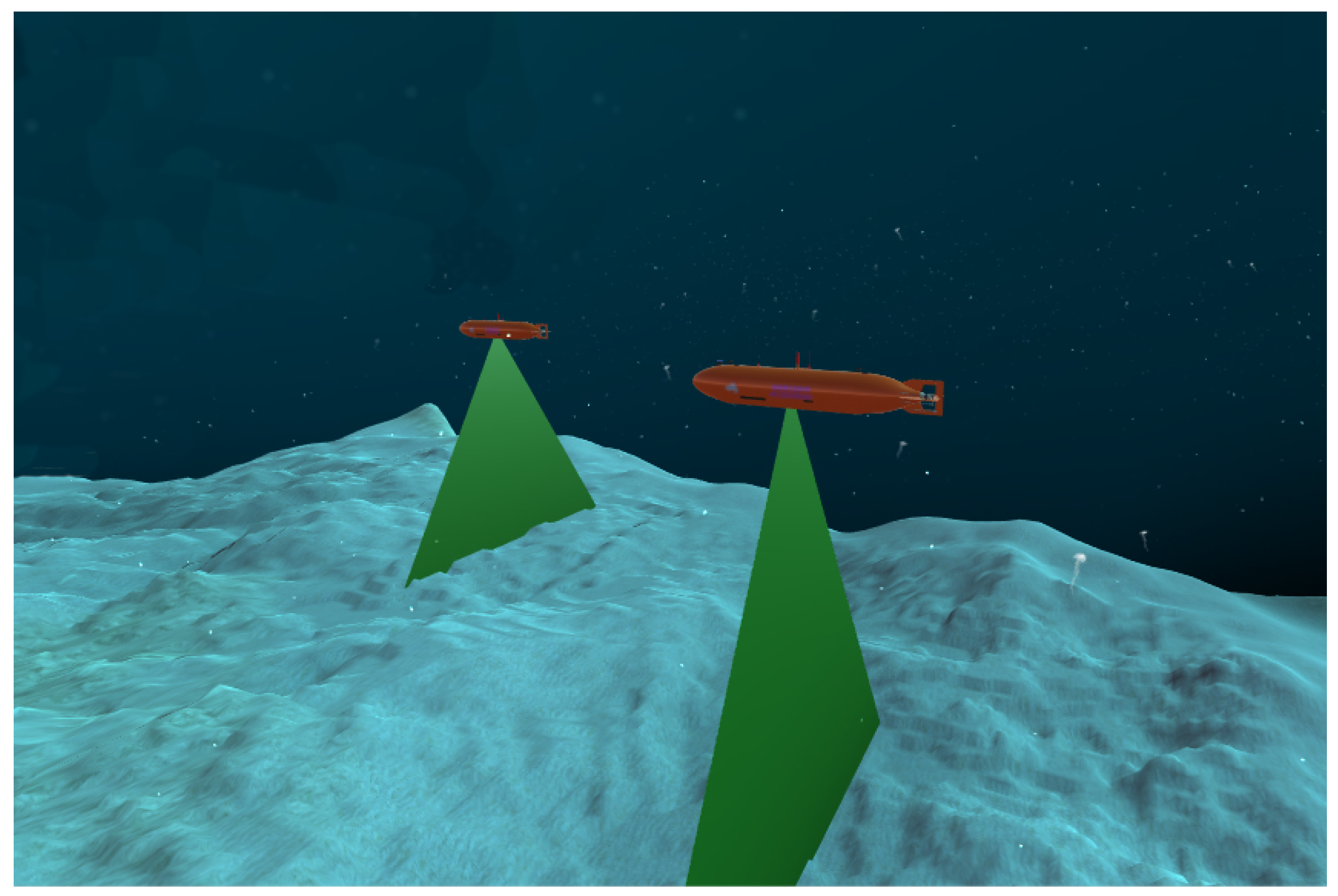
Figure 1 displays a typical situation in which Multiple Autonomous Underwater Vehicles (MAUVs) are used to discover underwater locations. Several AUVs equipped with underwater positioning equipment, including inertial navigation systems, multibeam sonars, and compass sensors, investigate the target region in this scenario. AUVs can only communicate with one another using underwater acoustic modems due to the lack of electromagnetic radiation in the underwater environment. This article examines ways to compress terrain data to a file size that can be sent through underwater acoustic modems.
The contribution of this paper has two main points:
1. This paper proposed a representation approach for multibeam bathymetry maps based on a quadtree structure. The quadtree structure storage depth map is able to better recover the 2.5-dimensional model, where the depth information is represented in two dimensions (x and y), while the third dimension (z) represents the depth, of seabed terrain detection, which, in turn, makes it possible for the map to take a lesser amount of storage space. Because the method described above for converting a gridded map to a quadtree map does not result in any loss of accuracy, the possibility that AUVs would use the map for collaborative SLAM is increased.
2. In order to compare and evaluate different compression algorithms (girding approach, SPGPs method, octree-based method, and the quadtree-based method presented here), as well as the compressed storage space and accuracy, several tests have been developed. These tests utilizes retrospective simulation to play back the dataset obtained by the authors during sea trials.
2. Related Wroks
2.1. Bathymetry Data Processing
Two 1300 km tracks of SEASAT altimeter data and related bathymetry are analyzed using the linear response function technique in the Musician Seamounts region north of Hawaii [
17]. An empirical method for predicting seafloor facies from multibeam bathymetry and acoustic backscatter data obtained in central Santa Monica Bay, California, has been developed [
18]. White [
19] investigate the effectiveness of linear and non-linear filtering techniques for removing impulse spikes from a digital bathymetry signal. The primary focus of [
20] is the compilation and editing of NOAA, individual scientists, SIO, NGA, JAMSTEC, IFREMER, GEBCO, and NAVOCEANO raw soundings. Merwade [
21] discusses the effect of spatial trend on isotropic interpolation algorithms. Uunk [
22] provide a fully automated method for deriving the daily intertidal beach bathymetry from video images of low-sloping beaches with intermittent intertidal bar emergence. Hasan [
23] predict the distribution of benthic biological habitats by integrating backscatter angular response with MBES bathymetry, backscatter mosaic, and their derivatives in a classification process using a random forests (RF) machine learning method. Using multi-temporal satellite pictures and random forest machine learning to generate a generic depth estimate model, a method for mapping shallow water bathymetry was devised [
24]. Guo used an airborne laser bathymetry (ALB) technology with digital full waveform signal collection to generate a bathymetry map from a full waveform echo signal [
25]. Wang described the quantitative approach of terrain suitability and the grid parameter solution method for optimal partition of suitable matching region [
26,
27], which increased the precision of terrain reference navigation navigation for AUVs.
2.2. Bathymetry Data Application
Bathymetry information has numerous applications. Lyons [
28] offer a method for mapping bathymetry and seagrass in shallow coastal waters by merging field survey data and high spatial resolution, multi-spectral satellite image data. Sembiring [
29] demonstrate the potential use of nearshore bathymetry calculated from video data in a coastal operational model for the Dutch Coast that forecasts daily waves, water levels, and rip currents. At Thorpeness, Suffolk, UK, Atkinson [
30] investigated the use of radar to derive nearshore bathymetry at a difficult site. Another important use of bathymetry data is terrain-matching navigation and bathymetry-based SALM. Ma expanded on AUV terrain matching navigation [
31], while Wang introduced estimate of confidence intervals to improve navigation precision [
32]. Cong [
33] and Ma [
34] suggested a technique for AUV path planning in terrain-aided navigation. Ma investigated the fundamentals of AUV robust bathymetric SLAM [
35] and presented a multi-window consistency method (MCM) to enhance the algorithm’s resilience [
36]. Zhang suggested using a particle filter for AUV bathymetric SLAM [
37,
38]. Ling presented an AUV active bathymetric SLAM approach [
39] that allows AUVs to choose their own routes for exhaustively exploring a region.
2.3. Multi-AUVs Detection
Due to the characteristics of the underwater environment, robot communication offers several challenges [
40]. Girod [
41] examine an acoustic ranging system that operates effectively in the face of several kinds of interference, but returns inaccurate results in non-line-of-sight settings. Adaptive Hybrid Automatic Repeat Request (HARQ) is used to provide reliable communications in the face of connection faults [
42]. Arun Kumar [
43,
44] proposes a kind of fog computing to improve the cloud computing of the Internet of Things, and provides a way to reduce energy consumption for multi-robot cooperative networking. Tsiogkas [
45] focused on the scientific field of underwater archaeology. Remmas [
46] discusses the management of a highly-maneuverable autonomous underwater vehicle for diver-tracking based on the data fusion of visual and audio signals recorded by low-cost sensors. Robotic cooperation and autonomy across many domains, autonomous mission planning, and the fusion of multi-domain data are described by Ross [
47]. Hilger examined the constraints of auditory communication in this respect in the realm of multi-AUV collaborative SLAM [
48]. Paull extracted landscape characteristics with an AUV equipped with side-scan sonar (SSS) [
13]. Ma employed multi-beam sonar terrain data to do this [
16], however employing SPGP’s approach to compress the map results in unclear map restoration problems.
3. System Definition
Considering the circumstance shown in
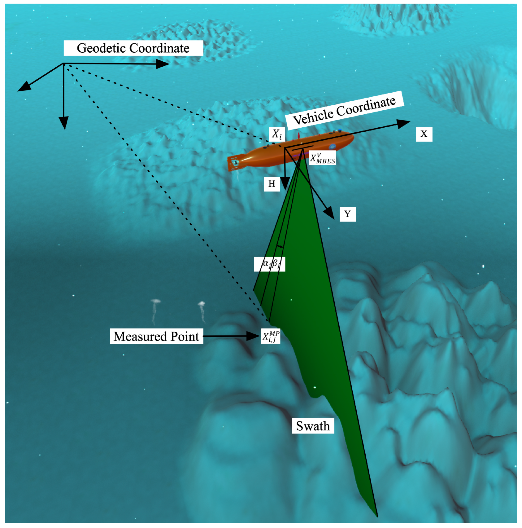
Figure 2, the AUV bathymetric detection system is specified. This system uses AUVs equipped with multibeam echo sonar (MBES) to measure the terrain of the bottom. AUVs navigate at the same depth to ensure optimal mapping precision and vehicle coverage.
are the states of the vehicle at consecutive instants of time
i where
is the number of states of the vehicle throughout the course of a mission. Dead reckoning (DR) systems are used to provide navigation data, including the vehicle’s control vectors
.
Bathymetric data obtained by MBES contains distances and angles (, where represents the number of beams broadcast by MBES) from the MBES head to the terrain, and the measured points are the sites where the beams hit the terrain. The horizontal locations () and terrain depths () of measured places at consecutive instants of time i may be calculated using bathymetric measurements collected with the MBES and related navigation data.
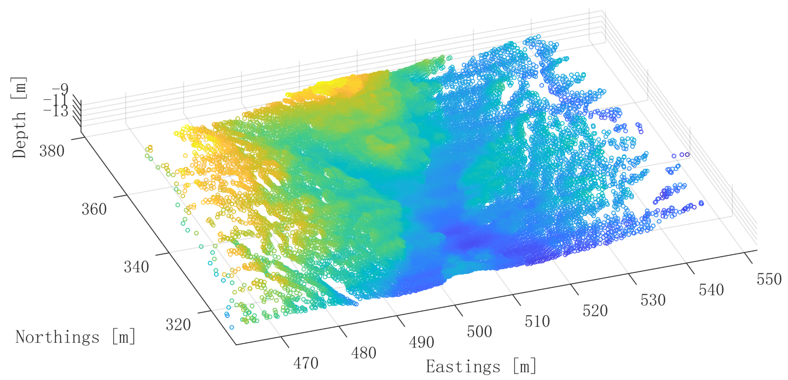
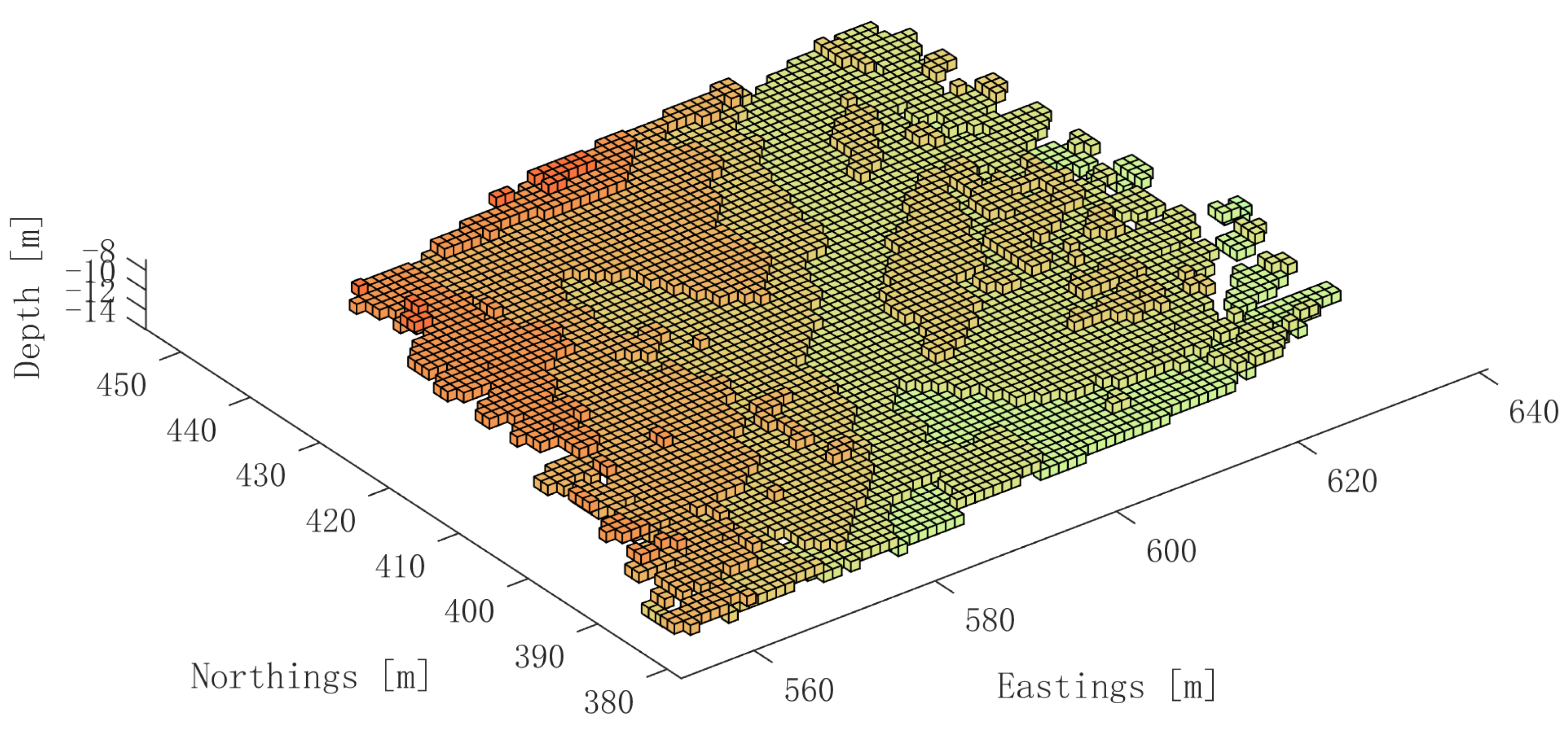
A 3D point cloud bathymetry map obtained by an AUV is seen in
Figure 3. The Eastings and Northings labels on the x and y axes reflect the geodetic coordinates used to measure location in the easting and northing directions, respectively. This map will used as an example in subsequent portions of the study.
In this bathymetric SLAM system, similar to a real multi-AUV cooperative detection situation, the sub-map incorporates bathymetric data and vehicle statuses, which the AUVs utilize for SLAM to produce exact maps while self-locating. Specifically, a sub-map comprises of a vehicle’s local trajectory plus a collection of swaths, with each swath including a significant number of measured points. The kth sub-maps created by the AUV are designated as (), where is the total number of sub-maps created by the AUV. When a vehicle creates a new sub-map, it will broadcast this sub-map using acoustic packets, and another vehicle will identify loop closures between this sub-map and all past sub-maps by recording these packets. After acquiring these loop closures, AUVs will complete SLAM using graph optimization algorithms or filtering algorithms.
4. Bathymetry Map Representation Method
4.1. Girding Approach
The Girding methodology has been thoroughly developed, and there are already numerous effective solutions. In the process of translating a point cloud map into a girding map, interpolation methods, such as Inverse Distance Weighting (IDW) [
49], Kriging [
50], and Natural Neighbor Interpolation (NNI) [
51] are often utilized. Using these techniques, the values of girding map cells are approximated based on the values of surrounding points within the point cloud data.
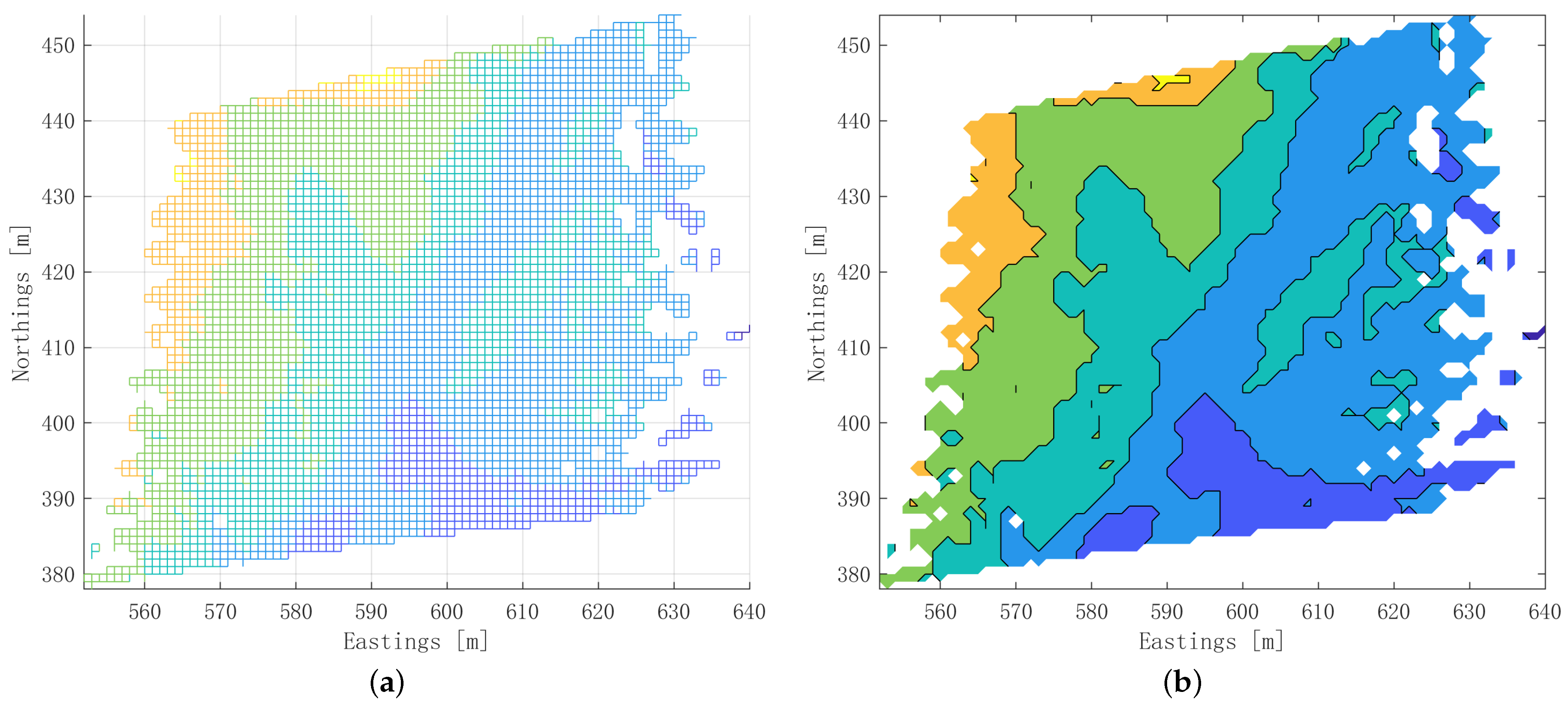
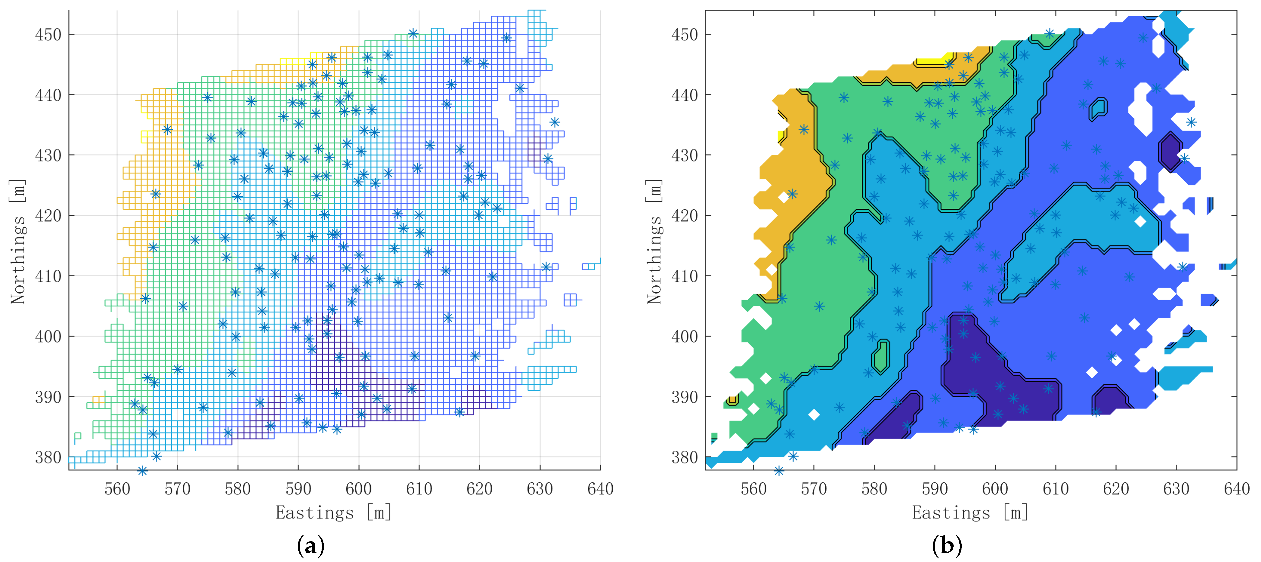
Figure 4a is a girding map converted from the test map (
Figure 3) using the girding approach.
Figure 4b is the contour map obtained from the girding map (
Figure 4a).
The girding technique can describe terrain depth maps fast and precisely, and it plays a significant role in the area of map storage. However, for the scenario of multi-AUVs cooperative detection, there is a greater need for storing space owing to the constraint of bandwidth. The girding map must be further compressed before it can be used, since its storage space is quite vast.
4.2. Sparse Pseudo-Input Gaussian Processes (SPGPs) Method
The sparse pseudo-input Gaussian processes (SPGPs) registration approach is used for registration and prediction by building an SPGPs model using historical data. Set of input points used to approximate the function being modeled by the Gaussian process. Instead of utilizing all of the training dataset’s input points, a subset of pseudo-points is chosen to represent the whole dataset. These pseudopoints are selected to offer a decent approximation of the function being modeled while minimizing the model’s computing expense. In contrast to conventional Gaussian processes registration (GPR) approaches, the SPGPs model is trained using just a limited number of pseudo points that retain the majority of the sub-map’s information, as opposed to all previous bathymetric data. Sub-maps may be sent if an AUV compresses the sub-map into certain pseudo points and calculates the hyperparameters of the SPGPs model associated with the sub-map, then the compressed sub-map is rebuilt in other AUVs.
The pseudo-point selection of SPGPs and associated theoretical derivation are available in Ma’s article [
16], thus they will not be duplicated here. Algorithm 1 is a proposed map compression algorithm utilizing SPGPs.
| Algorithm 1 Compression of Seafloor Terrain Maps using SPGPs |
| Require: Seafloor terrain maps, Pseudopoints |
| Ensure: Compressed terrain maps |
| 1: Train the SPGPs model using the pseudopoints |
| 2: Compute the mean and covariance function for each terrain map |
| 3: Predict the terrain maps based on the mean and covariance function |
| 4: for each terrain map do |
| 5: Compute the difference between the predicted terrain map and the actual terrain
map |
| 6: Store the difference in a separate variable |
| 7: end for |
| 8: Compress the difference variable |
| 9: Store the compressed difference variable along with the mean and covariance function
for each terrain map |
| 10: return The compressed terrain maps |
Figure 5a depicts the recovered map of the seafloor in the test map (
Figure 3), which was compressed using the SPGPs approach.
Figure 5b is the contour map obtained from the recovered map (
Figure 5a). In this scenario, 150 pseudo-input points are chosen. It is evident that the original map’s elevation change has been maintained, and that employing 150 points and hyperparameters to express the map may significantly minimize the amount of storage space required. However, this approach has the drawback of being a lossy compression method. A approach that is not only capable of lossless compression but also requires a modest amount of storage space may improve SLAM across various AUVs.
4.3. Octree-Based Method
The octree space occupancy approach for describing seafloor terrain maps is based on the concept of hierarchical spatial division. The octree approach breaks 3D space into progressively smaller cubes or octants, until each octant is tiny enough to reflect the terrain map’s depth. The octree map depicts the depth of the seabed topography via the occupancy of the three-dimensional space of the seabed.
In this approach, spatial partitioning is accomplished recursively, beginning with a single big cube that completely encloses the terrain map. The cube is then subdivided into eight smaller octants, each of which may be further subdivided if necessary. The leaf nodes of the octree structure hold data about the space filled by the seafloor terrain, whereas the non-leaf nodes store data regarding the occupancy of their children. Algorithm 2 depicts the algorithm flow.
Depending on the required resolution for a given application, several stop criteria may be configured. The objective of this research was to accomplish lossless compression of the gridded map, hence the stop criterion for the octree approach was set equal to the grid map resolution.
The octree space occupancy map created by the test map is shown in
Figure 6. When the voxel size of the octree map is sufficiently tiny (the same as the resolution of the girding map), it may be considered a lossless compression of the girding map. However, the map consumes a storage space of 10.8 kb, which surpasses the amount of data that AUVs can send in the time it takes to construct a submap (The bandwidth of high-performance underwater acoustic modems carried by the majority of AUVs is around 1000 bits per second. A data transfer of 10.8 kb per submap, which is equal to
88,473 bits and requires 88.47 s if sent by an AUV. Every 40 s, a new submap is formed, hence 10.8 kb is too huge to be sent by the existing AUVs). Therefore, this compression approach is not optimal for sharing maps between AUVs.
| Algorithm 2 Octree spatial occupancy method for representing seafloor terrain girding maps |
| Require: Seafloor terrain girding maps, voxel size, maximum tree depth |
| Ensure: The compressed octree representation of the seafloor terrain |
| 1: Convert each girding map into a voxel grid with the specified voxel size |
| 2: Initialize an octree with the maximum tree depth |
| 3: for each voxel in the voxel grid do |
| 4: if the voxel is occupied then |
| 5: CAdd the voxel into the octree |
| 6: end if |
| 7: end for |
| 8: Prune the octree by removing empty voxels and merging nearby occupied voxels |
| 9: Compress the octree by encoding the information of each node into a compact representation |
| 10: return The compressed octree representation of the seafloor terrain |
4.4. Quadtree-Based Method
A two-dimensional area is subdivided into four subregions according to the notion of describing seafloor topography maps using a quadtree structure. A node represents each subregion in the quadtree structure. This hierarchical technique efficiently represents sparse data by saving just the nodes that contain relevant information.
For terrain data, as illustrated in
Figure 7, the top-down building strategy is utilized. First, the whole landscape is treated as a node C0, which is at the minimum separation rate level. Divide into four child nodes C1, C2, C3, C4 of identical size; and the C1 node may be segmented into C5, C6, C7, C8.
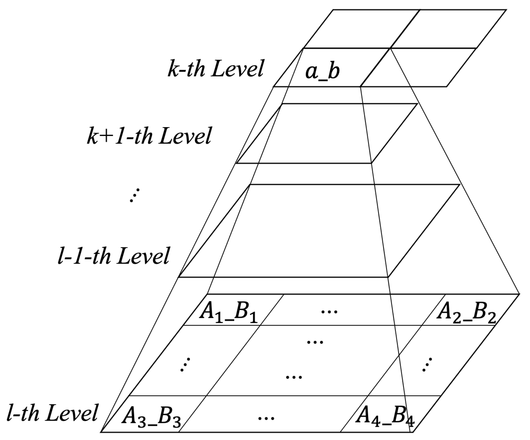
The number of data blocks rises with two to the
th power, where
n is the number of levels, as seen in the block hierarchical organizing technique (
Figure 8). If there is a data block
in the
kth layer, then the following formula may be used to determine the number
of all data blocks in the corresponding
l (
) layer:
Additionally, the names of the data blocks at the four corners of the
l (
) layer corresponding to
are
,
,
, and
, determined using the following formulas:
As seen in Algorithm 3, the premise of employing a quadtree approach to record seabed terrain maps requires encoding the maps as a hierarchical data structure in which each node corresponds to a square region on the map. The tree is formed by splitting the map into four squares of equal size, which serve as the current node’s children. This procedure is repeated until each leaf node represents a single square with identical seafloor terrain depth. Since the quadtree structure is separated into two-dimensional planes to store data, it resembles the 2.5D structure of the seabed topographic map, making it a more suitable way for map expression. In essence, the quadtree approach used in this work offers an alternate representation of a 2.5D grid-based map. The compression resolution is identical to that of the original gridded map, and so is the depth of each point in the resultant map. Thus, it is a form of lossless compression.
Table 1 summarizes the four algorithms from the theoretical level, including advantages and disadvantages, computational complexity and data storage requirement.
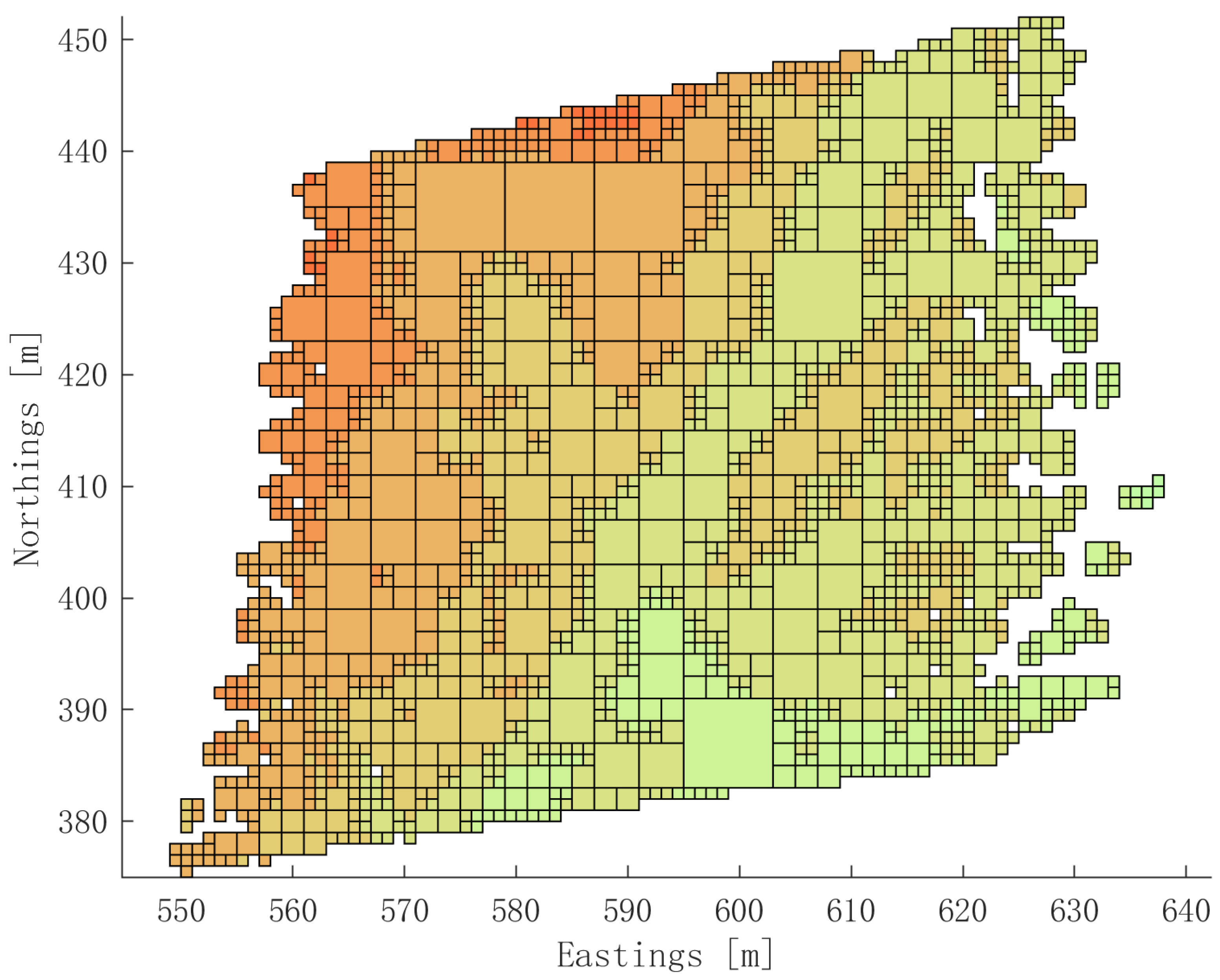
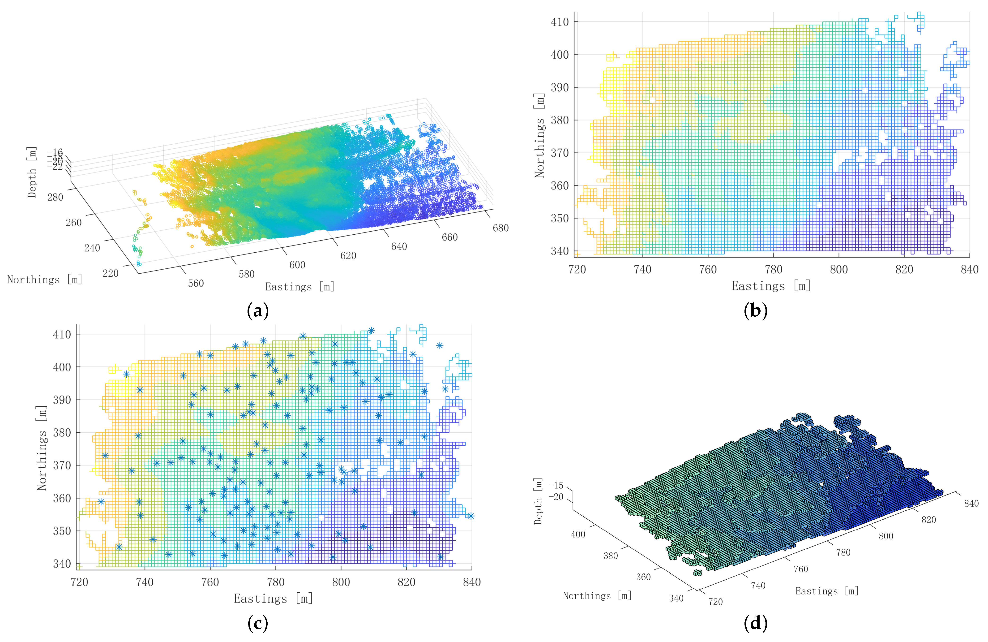
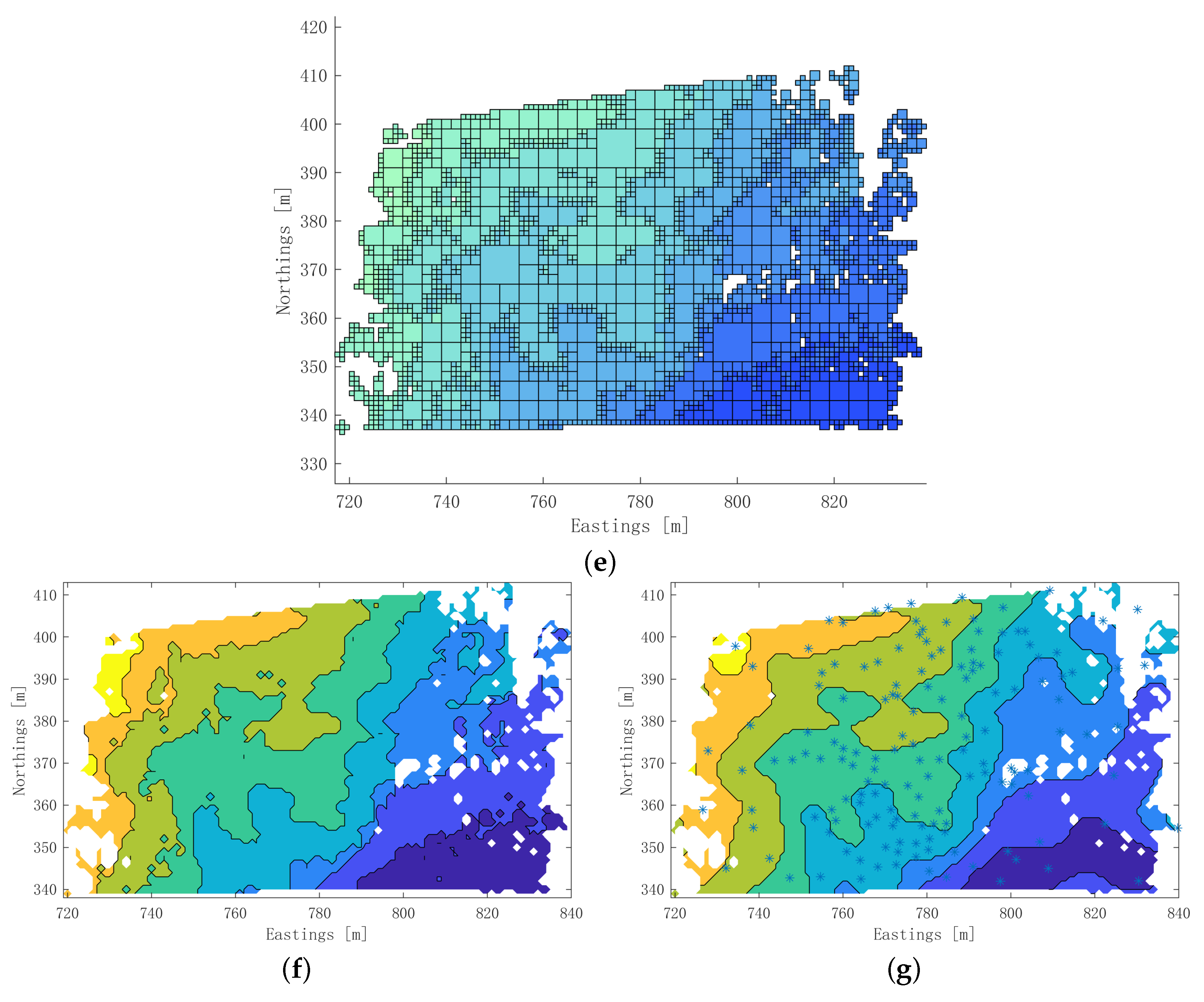
The quadtree representation map created by the test map is shown in
Figure 9. When the precision of the leaf node and the girding map are same, it may be considered a lossless compression of the girding map, similar to the octree map. In certain large regions with the same depth, the area is expressed by one or several large nodes, therefore conserving storage space. In certain huge regions with the same depth, the area is expressed by one or more large nodes, therefore conserving storage space. The map requires just 1936 bytes of storage space, allowing for its transmission.
| Algorithm 3 Quadtree representation of seabed terrain grid maps |
| Require: Terrain grid maps |
| Ensure: Quadtree representation of seabed terrain grid maps |
| 1: Initialize quadtree structure |
| 2: for each cell in the grid map do |
| 3: Assign cell value to corresponding node in quadtree |
| 4: Check if cell value satisfies subdivision criteria |
| 5: if subdivision criteria is satisfied then |
| 6: Subdivide node into 4 child nodes |
| 7: end if |
| 8: end for |
| 9: return Quadtree representation of seabed terrain grid maps |
5. Experiments and Settings
5.1. Datasets
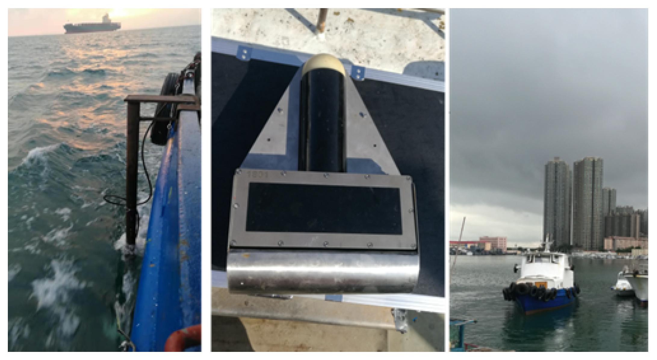
This section utilizes information from an experiment performed at sea near Qingdao, China. As shown in
Figure 10, a vessel equipped with multibeam sonar and INS devices was used to collect data from the East China Sea (
Figure 11).
Using two GNNS receivers of the XW-GI5651 INS/GNSS integrated navigation system mounted in the longitudinal portion of a vessel, the GPS trajectories of the vehicle were acquired. Using the system, the heading, pitch, and roll angles were measured with angular accuracies of O(), O(), and O(), respectively, at a frequency of 4 Hz.
In order to acquire bathymetric data, a shipborne T-sea CMBS200 MBSE operating at a frequency of 4 Hz was used. This sonar has a working bandwidth of 40 kHz and a center frequency of 200 kHz. It has a horizontal beamwidth of more than 1 degree and a vertical beamwidth of more than 2 degrees, both of which are remarkable. Horizontal field of vision larger than or equal to 140 degrees; detection range greater than or equal to 300 m; and distance resolution greater than or equal to 2 cm. In the experiment, 101 submaps were employed, including the test map used before (
Figure 3).
5.2. Map Compressing
In this work, we will assess the efficacy of four distinct compression techniques for displaying submaps of seabed landscape. In total, 101 maps have been chosen for compression testing. The objective is to evaluate and determine the most economical and effective compression technique for portraying complicated and high-resolution seabed landscape data. To guarantee a fair and thorough assessment, we will measure the performance of each technique using encoding time and storage utilization.
This research used a computer platform with the following specifications: an AMD Ryzen 3700X CPU, an NVIDIA GeForce RTX 2060 Super GPU, and 32 GB of DDR4 memory. This setup is adequate for the computing requirements of this study’s activities and is capable of giving dependable and efficient performance for the compression of seabed terrain maps. In addition, the machine is equipped with a 64-bit operating system and adequate storage space to support the datasets used in this research.
Under the multi-AUV cooperation situation, the robot will transmit the obtained submap. The acquisition time for each of the 101 submaps in the dataset is an average of 39.9 s, totaling 4030.5 s. Combining the performance of the already prevalent AUV underwater acoustic transmission modem (1000 bit/s), we determined the qualification line for the size of a single sub-map file after map compression to be 40,000 bit, or 5000 byte.
6. Results
In the experiment, 101 submaps were compressed using four different algorithms (Girding, SPGPs, Octree, Quadtree).
In addition to the previously used test map (
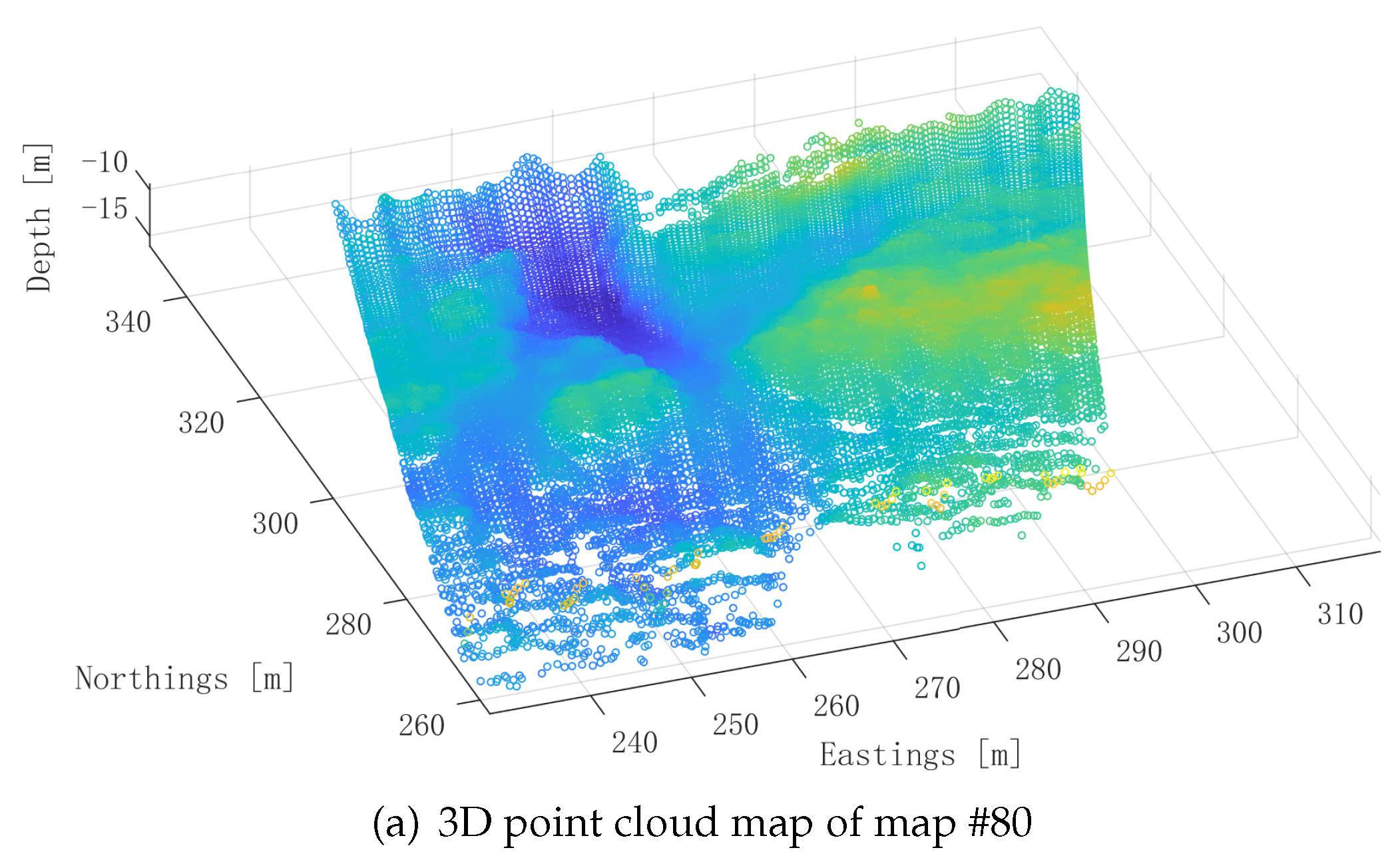
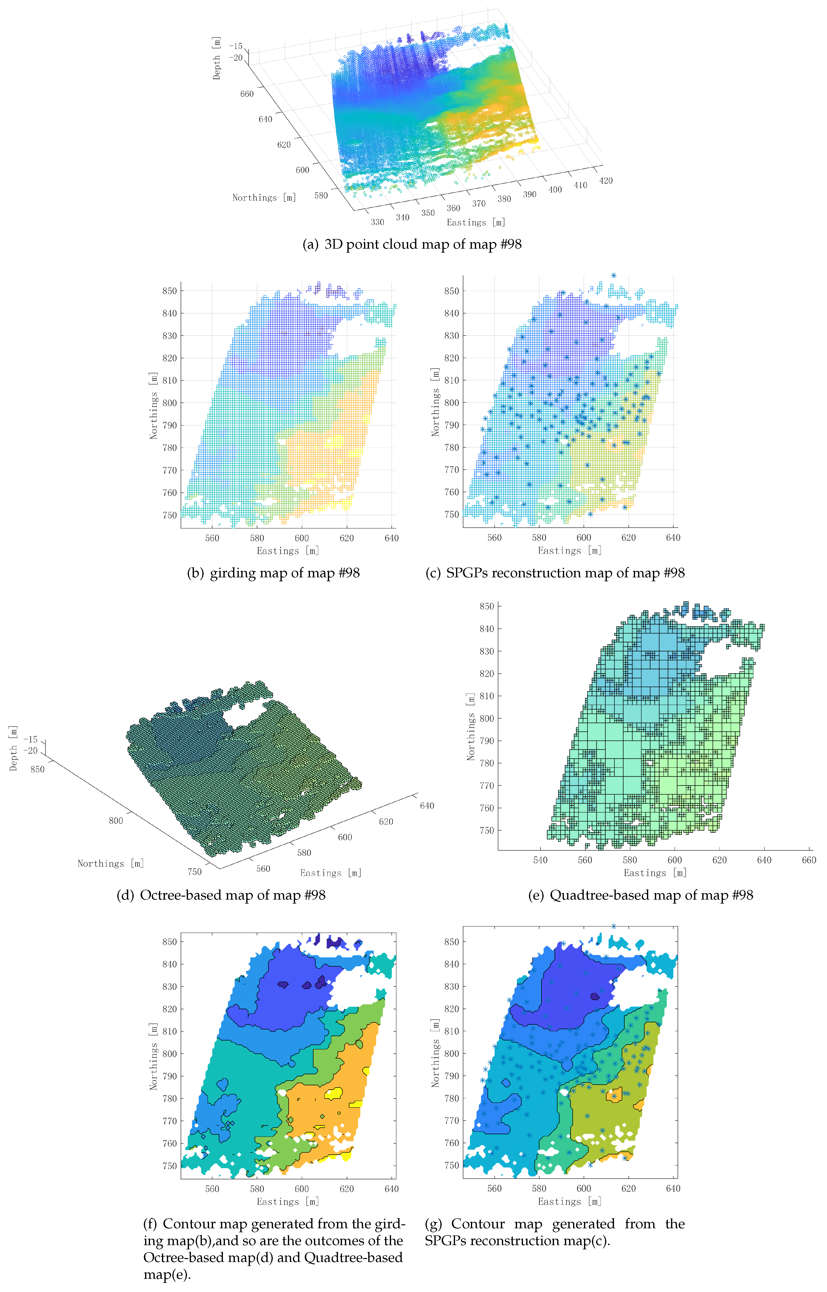
Figure 3), the test results of three maps (No. #74, #80, and #98) are shown as examples in
Figure 12,
Figure 13 and
Figure 14, respectively. It can be shown that, as predicted in the theoretical section, all four approaches can represent the seabed terrain depth map extremely effectively, among which SPGPs is a lossy compression, while the octree method and the quadtree method are lossless compression of the girding map.
In terms of disk space savings, the four methods vary significantly. According to
Figure 15 and
Table 2, the average space consumed by the four methods is 1 kilobyte, 2 kilobytes, 1 kilobyte, and 1 kilobyte, respectively. In the preceding section, a qualifying line was given in each submap of 5000 bytes, or 5 kb; hence, in multi-robot cooperation situations, only maps generated using SPGPs and quadtree map representation techniques may be sent out.
7. Discussion
Using improved techniques for underwater mapping has been a major field of study in recent years. The fundamental reason for selecting this subject was to improve the effectiveness of multi-robot cooperation for underwater research. By deploying numerous robots to collaborate, a larger area may be mapped in less time, and the mapping process as a whole can be quickened.
The approach presented for underwater mapping employs the quadtree structure. This approach may be used to compress maps, making it perfect for settings with limited storage capacity. Unfortunately, the quadtree structure technique, like the SPGPs method, has a significant computational cost.
This approach achieves lossless compression on the girding map since the same resolution as the girding map is employed. In other words, map reconstruction errors stem from the rasterization process and not the compression strategy. Experiments indicate the efficiency of the compression.
Considering the viability of using both techniques for deep-sea exploration, both techniques may be used with certain considerations. For instance, underwater communication is possible using acoustic modems. Nevertheless, the performance of these modems must be considered to guarantee that the maps can be sent between AUVs effectively. In addition, the high computational cost of these approaches may not be a serious concern in deep water research since newer AUVs are equipped with strong processors capable of performing complicated computations.
8. Conclusions
In this study, a representation method for multibeam bathymetry maps based on a quadtree structure was developed. The following conclusions can be drawn:
1. The bathymetric map of the seafloor may be compressed and restored using the suggested quadtree structure-based method.
2. This approach requires less disk space than the existing method and can also assure map accuracy. The average size of the 101 sub-maps employed in the experiment is 2571 bytes, making it feasible to transfer maps across AUVs.
By using offered techniques for underwater mapping has the potential to considerably improve the effectiveness of underwater exploration. Although the suggested approaches provide a number of benefits, including a reduction in map storage needs, the high computational cost may be a disadvantage. Additionally though, with the developments of AUV technology and underwater communication, these techniques may be used to explore the deep oceans.
In future study, we will examine the performance of multi-AUV collaborative SLAM systems after transmitting compressed maps using this compression approach, as well as other relevant studies.
Author Contributions
Conceptualization, Z.C. and T.M.; methodology, Z.C. and Y.L. (Yu Ling); software, Z.C. and H.D.; validation, Y.L. (Ye Li), Z.L., C.Q. and T.M.; investigation, Y.L. (Ye Li), Z.C., Q.Z., S.X. and T.M.; resources, Y.L. (Ye Li) and T.M.; writing—original draft preparation, Z.C.; writing—review and editing, Y.L. (Ye Li) and T.M.; visualization, H.D., Y.L. (Yu Ling) and M.Y.; supervision, Y.L. (Ye Li) and T.M.; funding acquisition, Y.L. (Ye Li) and T.M. All authors have read and agreed to the published version of the manuscript.
Funding
This work was supported in part by Hainan Provincial Joint Project of Sanya Yazhou Bay Science and Technology City, Grant No: 520LH006; in part by the National Natural Science Foundation of China under Grant 52001093; in part by the High-level scientific research guidance project of Harbin Engineering University, under Grant 3072022TS0102.
Institutional Review Board Statement
Not applicable.
Informed Consent Statement
Not applicable.
Data Availability Statement
Not applicable.
Conflicts of Interest
The authors declare no conflict of interest.
References
- Maurelli, F.; Krupiński, S.; Xiang, X.; Petillot, Y. AUV localisation: A review of passive and active techniques. Int. J. Intell. Robot. Appl. 2021, 6, 1–24. [Google Scholar] [CrossRef]
- Chen, P.; Li, Y.; Su, Y.; Chen, X.; Jiang, Y. Review of AUV underwater terrain matching navigation. J. Navig. 2015, 68, 1155–1172. [Google Scholar] [CrossRef]
- Paull, L.; Saeedi, S.; Seto, M.; Li, H. AUV navigation and localization: A review. IEEE J. Ocean. Eng. 2013, 39, 131–149. [Google Scholar] [CrossRef]
- Edge, C.; Enan, S.S.; Fulton, M.; Hong, J.; Mo, J.; Barthelemy, K.; Bashaw, H.; Kallevig, B.; Knutson, C.; Orpen, K.; et al. Design and experiments with LoCO AUV: A low cost open-source autonomous underwater vehicle. In Proceedings of the 2020 IEEE/RSJ International Conference on Intelligent Robots and Systems (IROS), Las Vegas, NV, USA, 24 October 2020–24 January 2021; pp. 1761–1768. [Google Scholar]
- Yan, J.; Ban, H.; Luo, X.; Zhao, H.; Guan, X. Joint localization and tracking design for AUV with asynchronous clocks and state disturbances. IEEE Trans. Veh. Technol. 2019, 68, 4707–4720. [Google Scholar] [CrossRef]
- Zhao, W.; He, T.; Sani, A.Y.M.; Yao, T. Review of slam techniques for autonomous underwater vehicles. In Proceedings of the 2019 International Conference on Robotics, Intelligent Control and Artificial Intelligence, Shanghai, China, 20–22 September 2019; pp. 384–389. [Google Scholar]
- Ouyang, X.; Zeng, F.; Lv, D.; Dong, T.; Wang, H. Cooperative Navigation of UAVs in GNSS-Denied Area With Colored RSSI Measurements. IEEE Sens. J. 2021, 21, 2194–2210. [Google Scholar] [CrossRef]
- Özkahraman, Ö.; Ögren, P. Collaborative Navigation-Aware Coverage in Feature-Poor Environments. In Proceedings of the 2022 IEEE/RSJ International Conference on Intelligent Robots and Systems (IROS), Kyoto, Japan, 23–27 October 2022; pp. 10066–10073. [Google Scholar]
- Luvisutto, A.; Miolato, M.; AlMaleki, O.; Al Marzooqi, A.; Traversi, E.; De Masi, G. Advanced Modeling Techniques for Mission Planning of Marine Multi-Vehicles systems: What’s Next? In Proceedings of the OCEANS 2022, Chennai, India, 21–24 February 2022; pp. 1–6. [Google Scholar]
- Schmidt, H.; Leonard, J. GOATS’2002, Multi-AUV Cooperative Behavior for Littoral MCM and REA Concurrent Mapping and Localization; Technical Report; Massachusetts Institute of Technology: Cambrigde, MA, USA, 2002. [Google Scholar]
- Zhang, S.; Zhao, S.; An, D.; Liu, J.; Wang, H.; Feng, Y.; Li, D.; Zhao, R. Visual SLAM for underwater vehicles: A survey. Comput. Sci. Rev. 2022, 46, 100510. [Google Scholar] [CrossRef]
- Fallon, M.F.; Kaess, M.; Johannsson, H.; Leonard, J.J. Efficient AUV navigation fusing acoustic ranging and side-scan sonar. In Proceedings of the 2011 IEEE International Conference on Robotics and Automation, Shanghai, China, 9–13 May 2011; pp. 2398–2405. [Google Scholar]
- Paull, L.; Huang, G.; Seto, M.; Leonard, J.J. Communication-constrained multi-AUV cooperative SLAM. In Proceedings of the 2015 IEEE international conference on robotics and automation (ICRA), Seattle, WA, USA, 26–30 May 2015; pp. 509–516. [Google Scholar]
- Yang, Y.; Xiao, Y.; Li, T. A survey of autonomous underwater vehicle formation: Performance, formation control, and communication capability. IEEE Commun. Surv. Tutorials 2021, 23, 815–841. [Google Scholar] [CrossRef]
- Palomer, A.; Ridao, P.; Ribas, D.; Mallios, A.; Vallicrosa, G. Octree-based subsampling criteria for bathymetric SLAM. In Proceedings of the XXXV Jornadas de Automática, Valencia, Spain, 3–5 September 2014; pp. 3–5. [Google Scholar]
- Ma, T.; Zhang, W.; Li, Y.; Zhao, Y.; Zhang, Q.; Mei, X.; Fan, J. Communication-constrained cooperative bathymetric simultaneous localisation and mapping with efficient bathymetric data transmission method. J. Navig. 2022, 75, 1000–1016. [Google Scholar] [CrossRef]
- Dixon, T.H.; Naraghi, M.; McNutt, M.; Smith, S. Bathymetric prediction from Seasat altimeter data. J. Geophys. Res. Ocean. 1983, 88, 1563–1571. [Google Scholar] [CrossRef]
- Dartnell, P.; Gardner, J.V. Predicting seafloor facies from multibeam bathymetry and backscatter data. Photogramm. Eng. Remote Sens. 2004, 70, 1081–1091. [Google Scholar] [CrossRef] [Green Version]
- White, L.; Hodges, B.R. Filtering the signature of submerged large woody debris from bathymetry data. J. Hydrol. 2005, 309, 53–65. [Google Scholar] [CrossRef]
- Becker, J.; Sandwell, D.; Smith, W.; Braud, J.; Binder, B.; Depner, J.; Fabre, D.; Factor, J.; Ingalls, S.; Kim, S.; et al. Global bathymetry and elevation data at 30 arc seconds resolution: SRTM30_PLUS. Mar. Geod. 2009, 32, 355–371. [Google Scholar] [CrossRef]
- Merwade, V. Effect of spatial trends on interpolation of river bathymetry. J. Hydrol. 2009, 371, 169–181. [Google Scholar] [CrossRef]
- Uunk, L.; Wijnberg, K.M.; Morelissen, R. Automated mapping of the intertidal beach bathymetry from video images. Coast. Eng. 2010, 57, 461–469. [Google Scholar] [CrossRef]
- Che Hasan, R.; Ierodiaconou, D.; Laurenson, L.; Schimel, A. Integrating multibeam backscatter angular response, mosaic and bathymetry data for benthic habitat mapping. PLoS ONE 2014, 9, e97339. [Google Scholar] [CrossRef] [Green Version]
- Sagawa, T.; Yamashita, Y.; Okumura, T.; Yamanokuchi, T. Satellite derived bathymetry using machine learning and multi-temporal satellite images. Remote Sens. 2019, 11, 1155. [Google Scholar] [CrossRef] [Green Version]
- Guo, K.; Li, Q.; Wang, C.; Mao, Q.; Liu, Y.; Ouyang, Y.; Feng, Y.; Zhu, J.; Wu, A. Target Echo Detection Based on the Signal Conditional Random Field Model for Full-Waveform Airborne Laser Bathymetry. IEEE Trans. Geosci. Remote Sens. 2022, 60, 1–21. [Google Scholar] [CrossRef]
- Rupeng, W.; Ye, L.; Teng, M.; Zheng, C.; Yusen, G. Underwater digital elevation map gridding method based on optimal partition of suitable matching area. Int. J. Adv. Robot. Syst. 2019, 16, 1729881418824833. [Google Scholar] [CrossRef] [Green Version]
- Rupeng, W.; Ye, L.; Teng, M.; Zheng, C.; Yusen, G.; Yanqing, J.; Qiang, Z. A new model and method of terrain-aided positioning confidence interval estimation. J. Mar. Sci. Technol. 2021, 27, 27–39. [Google Scholar] [CrossRef]
- Lyons, M.; Phinn, S.; Roelfsema, C. Integrating Quickbird multi-spectral satellite and field data: Mapping bathymetry, seagrass cover, seagrass species and change in Moreton Bay, Australia in 2004 and 2007. Remote Sens. 2011, 3, 42–64. [Google Scholar] [CrossRef] [Green Version]
- Sembiring, L.; Van Dongeren, A.; Winter, G.; Van Ormondt, M.; Briere, C.; Roelvink, D. Nearshore bathymetry from video and the application to rip current predictions for the Dutch Coast. J. Coast. Res. 2014, 70, 354–359. [Google Scholar] [CrossRef]
- Atkinson, J.; Esteves, L.S.; Williams, J.W.; McCann, D.L.; Bell, P.S. The application of X-band radar for characterization of nearshore dynamics on a mixed sand and gravel beach. J. Coast. Res. 2018, 85, 281–285. [Google Scholar] [CrossRef]
- Teng, M.; Ye, L.; Yuxin, Z.; Yanqing, J.; Zheng, C.; Qiang, Z.; Shuo, X. An AUV localization and path planning algorithm for terrain-aided navigation. ISA Trans. 2020, 103, 215–227. [Google Scholar] [CrossRef] [PubMed]
- Rupeng, W.; Ye, L.; Teng, M.; Zheng, C.; Yusen, G.; Pengfei, X. Improvements to terrain aided navigation accuracy in deep-sea space by high precision particle filter initialization. IEEE Access 2019, 8, 13029–13042. [Google Scholar] [CrossRef]
- Cong, Z.; Li, Y.; Jiang, Y.; Ma, T.; Gong, Y.; Wang, R.; Wu, H. An evaluation of path-planning methods for autonomous underwater vehicle based on terrain-aided navigation. Int. J. Adv. Robot. Syst. 2019, 16, 1729881419853181. [Google Scholar] [CrossRef] [Green Version]
- Teng, M.; Ye, L.; Yanqing, J.; Rupeng, W.; Zheng, C.; Yusen, G. A dynamic path planning method for terrain-aided navigation of autonomous underwater vehicles. Meas. Sci. Technol. 2018, 29, 095105. [Google Scholar] [CrossRef]
- Ma, T.; Li, Y.; Wang, R.; Cong, Z.; Gong, Y. AUV robust bathymetric simultaneous localization and mapping. Ocean. Eng. 2018, 166, 336–349. [Google Scholar] [CrossRef]
- Teng, M.; Ye, L.; Yuxin, Z.; Zhang, Q.; Jiang, Y.; Zheng, C.; Zhang, T. Robust bathymetric SLAM algorithm considering invalid loop closures. Appl. Ocean. Res. 2020, 102, 102298. [Google Scholar]
- Zhang, Q.; Li, Y.; Ma, T.; Cong, Z.; Zhang, W. Bathymetric particle filter SLAM based on mean trajectory map representation. IEEE Access 2021, 9, 71725–71736. [Google Scholar] [CrossRef]
- Zhang, Q.; Li, Y.; Ma, T.; Cong, Z.; Zhang, W. Bathymetric particle filter SLAM with graph-based trajectory update method. IEEE Access 2021, 9, 85464–85475. [Google Scholar] [CrossRef]
- Ling, Y.; Li, Y.; Ma, T.; Cong, Z.; Xu, S.; Li, Z. Active Bathymetric SLAM for autonomous underwater exploration. Appl. Ocean. Res. 2023, 130, 103439. [Google Scholar] [CrossRef]
- Maurelli, F.; Saigol, Z.; Insaurralde, C.C.; Petillot, Y.R.; Lane, D.M. Marine world representation and acoustic communication: Challenges for multi-robot collaboration. In Proceedings of the 2012 IEEE/OES Autonomous Underwater Vehicles (AUV), Southampton, UK, 24–27 September 2012; pp. 1–6. [Google Scholar]
- Girod, L.; Estrin, D. Robust range estimation using acoustic and multimodal sensing. In Proceedings of the IEEE/RSJ International Conference on Intelligent Robots and Systems, Expanding the Societal Role of Robotics in the the Next Millennium (Cat. No. 01CH37180), Maui, HI, USA, 29 October–3 November 2001; Volume 3, pp. 1312–1320. [Google Scholar]
- Rahmati, M.; Petroccia, R.; Pompili, D. In-network collaboration for CDMA-based reliable underwater acoustic communications. IEEE J. Ocean. Eng. 2019, 44, 881–894. [Google Scholar] [CrossRef] [Green Version]
- Kumar, A.; Sharma, S.; Goyal, N.; Singh, A.; Cheng, X.; Singh, P. Secure and energy-efficient smart building architecture with emerging technology IoT. Comput. Commun. 2021, 176, 207–217. [Google Scholar] [CrossRef]
- Kumar, A.; Sharma, S.; Goyal, N.; Gupta, S.K.; Kumari, S.; Kumar, S. Energy-efficient fog computing in Internet of Things based on Routing Protocol for Low-Power and Lossy Network with Contiki. Int. J. Commun. Syst. 2022, 35, e5049. [Google Scholar] [CrossRef]
- Tsiogkas, N.; Frost, G.; Monni, N.; Lane, D. Facilitating multi-AUV collaboration for marine archaeology. In Proceedings of the OCEANS 2015, Washington, DC, USA, 19–22 October 2015; pp. 1–4. [Google Scholar]
- Remmas, W.; Chemori, A.; Kruusmaa, M. Diver tracking in open waters: A low-cost approach based on visual and acoustic sensor fusion. J. Field Robot. 2021, 38, 494–508. [Google Scholar] [CrossRef]
- Ross, J.; Lindsay, J.; Gregson, E.; Moore, A.; Patel, J.; Seto, M. Collaboration of multi-domain marine robots towards above and below-water characterization of floating targets. In Proceedings of the 2019 IEEE International Symposium on Robotic and Sensors Environments (ROSE), Ottawa, ON, Canada, 17–18 June 2019; pp. 1–7. [Google Scholar]
- Hilger, R.P. Acoustic Communications Considerations for Collaborative Simultaneous Localization and Mapping; Technical Report; Naval Postgraduate School: Monterey, CA, USA, 2014. [Google Scholar]
- Lu, G.Y.; Wong, D.W. An adaptive inverse-distance weighting spatial interpolation technique. Comput. Geosci. 2008, 34, 1044–1055. [Google Scholar] [CrossRef]
- Mueller, T.; Pusuluri, N.; Mathias, K.; Cornelius, P.; Barnhisel, R.; Shearer, S. Map quality for ordinary kriging and inverse distance weighted interpolation. Soil Sci. Soc. Am. J. 2004, 68, 2042–2047. [Google Scholar] [CrossRef]
- Beutel, A.; Mølhave, T.; Agarwal, P.K. Natural neighbor interpolation based grid DEM construction using a GPU. In Proceedings of the 18th SIGSPATIAL International Conference on Advances in Geographic Information Systems, San Jose, CA, USA, 2–5 November 2010; pp. 172–181. [Google Scholar]
| Disclaimer/Publisher’s Note: The statements, opinions and data contained in all publications are solely those of the individual author(s) and contributor(s) and not of MDPI and/or the editor(s). MDPI and/or the editor(s) disclaim responsibility for any injury to people or property resulting from any ideas, methods, instructions or products referred to in the content. |
© 2023 by the authors. Licensee MDPI, Basel, Switzerland. This article is an open access article distributed under the terms and conditions of the Creative Commons Attribution (CC BY) license (https://creativecommons.org/licenses/by/4.0/).


 ,
, 


