
Influences of Gap Flow on Air Resistance Acting on a Large Container Ship

1
Faculty of Transportation Mechanical Engineering, University of Science and Technology—The University of Danang, Danang 550000, Vietnam
2
Department of Marine System Engineering, Graduate School of Engineering, Osaka Metropolitan University, Sakai, Osaka 599-8531, Japan
*
Author to whom correspondence should be addressed.
J. Mar. Sci. Eng. 2023, 11(1), 160; https://doi.org/10.3390/jmse11010160
Submission received: 8 December 2022
/
Revised: 20 December 2022
/
Accepted: 31 December 2022
/
Published: 9 January 2023
(This article belongs to the Section Ocean Engineering)
Abstract
:In terms of speed lost and fuel consumed, wind loads are considered one of the main factors for large ship design, especially for container ships. Alongside water resistance, air resistance in strong wind conditions has a significant impact on the fuel efficiency and performance of container ships with large box-type bodies. This paper reports the effects of wind loads acting on a 20,000 TEU container ship carrying large numbers of deck containers using a commercial CFD software program (ANSYS Fluent V14.5 with RANS equation). A 1/255.3 scale model was used in this study to reveal the air resistance on the container ship configuration. The aerodynamic formations of the complex vortices, pressure, velocity contours, and streamlines, as well as the air forces acting on the container ship, are presented and discussed. The pressure distributions show that the gap air flows increase the stagnation pressure at the face side and decrease the pressure on the backside of each container gap through separate eddies. The difference in pressures created in the gaps contribute to the air resistance acting on the ship. It is confirmed that the use of side covers of deck containers to close the gap flows between container blocks can significantly reduce the air resistance for wind directions in the range of 30 to 60 degrees.
1. Introduction
Economic and environmental considerations are two great concerns for any industrial ship design, especially, in terms of lost speed and high fuel consumption [1,2,3,4,5]. As the ship is cruising, the resistances acting on a ship consist of water resistance and air resistance [6]. Typically, for small ships, the air resistance is relatively smaller than the water resistance and can be considered a minor factor in the total resistance [7]. However, for large ships, the wind force is proportional to the projected area of the upper structures above the water and the square of the wind speed. For ships with a large projected area running in a strong wind, air resistance becomes a significant factor and cannot be neglected [8,9,10]. Therefore, how to minimize air resistance has become an important issue for such large ships. To reduce the wind force acting on a non-ballasted ship, Sugata experimentally studied the air resistance using three new types of superstructures including a conventional shape, a lower shape, and a streamlined shape [11]. The experimental study showed that the longitudinal wind force of the ship with the streamlined superstructure decreases by 44% in the fully loaded condition and by 33% in the non-ballast condition in the headwind. In addition, the lateral force decreases by about 30% for the streamlined design.
Air resistance acting on ships has been investigated broadly to reduce fuel consumption and increase ship performance [12,13]. For instance, to provide directly applicable results for container-ship operators and to provide benchmark values for the development of new computational methods, Andersen investigated the effect of container configurations on the wind load by carrying out experimental tests in a wind tunnel [14]. The recommendation to reduce the longitudinal force is to make the configuration as smooth as possible; streamlining can also reduce the longitudinal force for headwinds. Ouchi studied the reduction of the air drag acting on the 6700 TEU over-Panamax container ship in the sea using experimental and numerical methods [15]. The results showed that by setting devices on the deck for smoothing the airflow and arranging the storage, the air resistance can be reduced appropriately. Kim evaluated the design and performance of superstructure modification for reducing the air drag of a container ship [16] Several design concepts and devices on the superstructure of a container ship were suggested to reduce air drag. Gap protectors between container stacks and a visor in front of the upper deck were presented as the most effective way to improve drag reduction for a wide range of heading angles. RANS computations were carried out for three model configurations and compared with the experimental data. A numerical study on reducing the air resistance acting on a ship has been presented using interaction effects between the hull and accommodation [17,18]. The computational results showed that the shape and position of the accommodation on the ship significantly influenced air resistance. In addition, the air resistance acting on a large container ship running in the headwind was reduced by controlling vortices generated at the bow and around the containers on deck. Watanabe et al. [19] experimentally tested methods to reduce air resistance for a scale model of a 20,000 TEU container ship with containers on deck and developed several configurations to reduce air resistance. However, in oblique winds, the airflow passing over the ship becomes more complex because of the existence of many gaps between the deck containers. Although the reduction in air resistance occurring in large container ships has been extensively researched, as in the aforementioned studies, the characteristics of the airflow in gaps between containers have not yet been fully clarified.
Extending the previous study proposed by Watanabe et. al., and Nguyen et al. [19,20], the present study investigates the airflow passing the gaps between container blocks on deck by applying CFD and describes how to control the flow to reduce the air resistance acting on the ship. The CFD results are compared with experimental data obtained from open wind tunnel tests at Osaka Prefecture University [19] and provide the characteristics of the airflow passing a large container ship.
Although in some specific situations of bad weather, a large container ship might not be able to use side covers because the resulting variable loading would affect the safety of the ship, this study considers the normal conditions of weather and full loading of containers on deck to understand the effects of using side covers on reducing the air resistance and provide the flow characteristics over large container ships in the cases of headwinds and oblique winds.
2. Numerical Method
The characteristics of the airflow passing a large container ship are numerically investigated. The computational processes are explained in the following section.
2.1. CAD Modeling
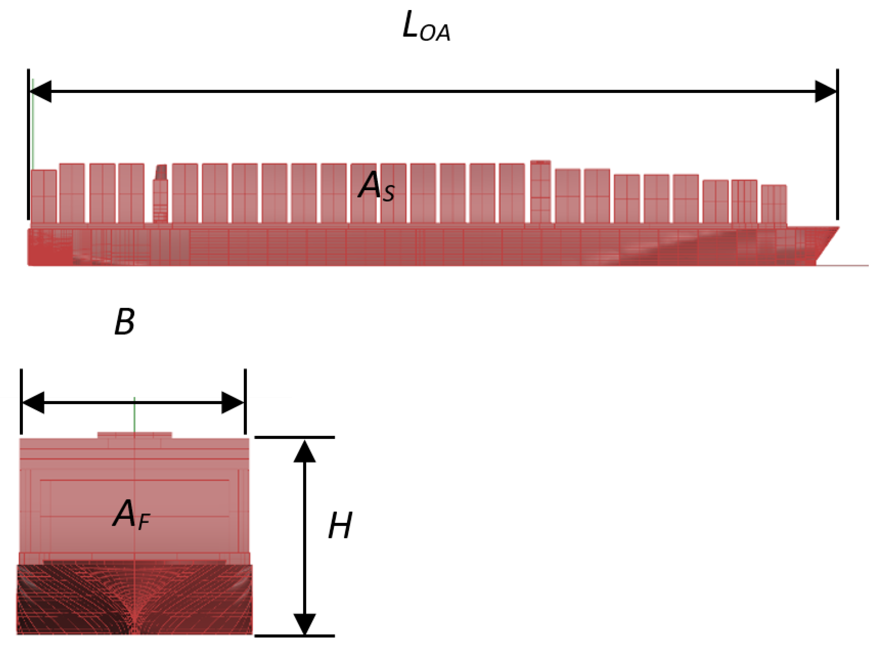
In this study, the same container ship model proposed by Watanabe [19] is used for the simulations. The present CFD calculations are validated using Watanabe’s experimental results. The principal particulars of the 20,000 TEU container ship and its scale model are presented in Table 1. The side and frontal views of the model with deck containers in the fully loaded condition are shown in Figure 1. In the figure, AF is the frontal projected area of the container ship while AS is the side projected area excluding the gaps.
2.2. Computational Fluid Dynamics (CFD)
A commercial CFD software program, ANSYS Fluent V14.5, is used to solve the Reynolds-Averaged Navier-Stokes (RANS) equations for incompressible turbulent flow.
RANS equations are time-averaged equations obtained by decomposing the variables in the instantaneous NS equations into mean (ensemble-averaged or time-averaged) and fluctuation components. Replacing the instantaneous variables with the sum of the mean and the fluctuation components and taking an ensemble average or time average yields the RANS equations [21]:
where and are the mean velocity and mean pressure, and are the fluctuating components and is the mean strain-rate tensor:
The computational domain, mesh generation, and numerical setup are shown in the following sections.
2.2.1. Computational Domain
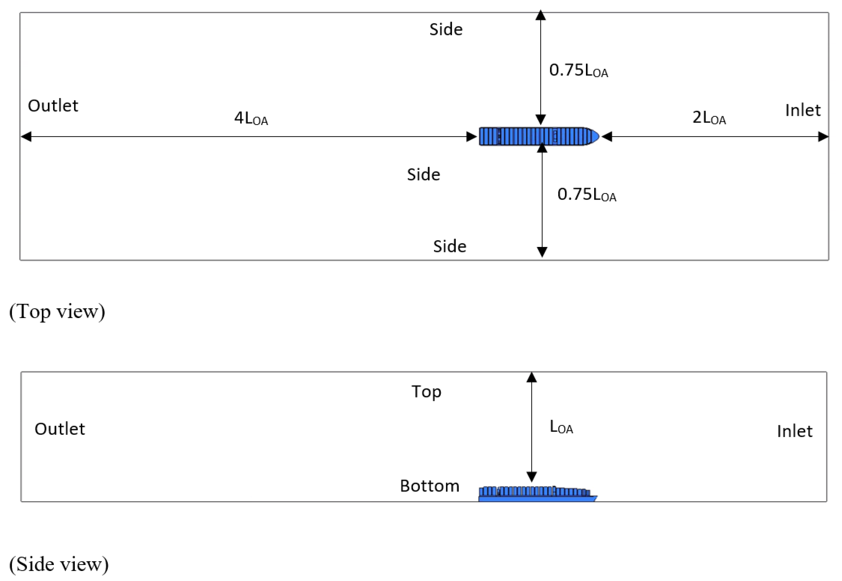
The computational domain for CFD simulation used ITTC recommendation [22] and is shown in Figure 2. The upstream and downstream distances are 2 × LOA and 4 × LOA, respectively, where LOA is the overall length of the ship. The distances to the sidewalls and top wall from the model are 0.75 × LOA and LOA, respectively.
2.2.2. Coordinate System and Coefficients
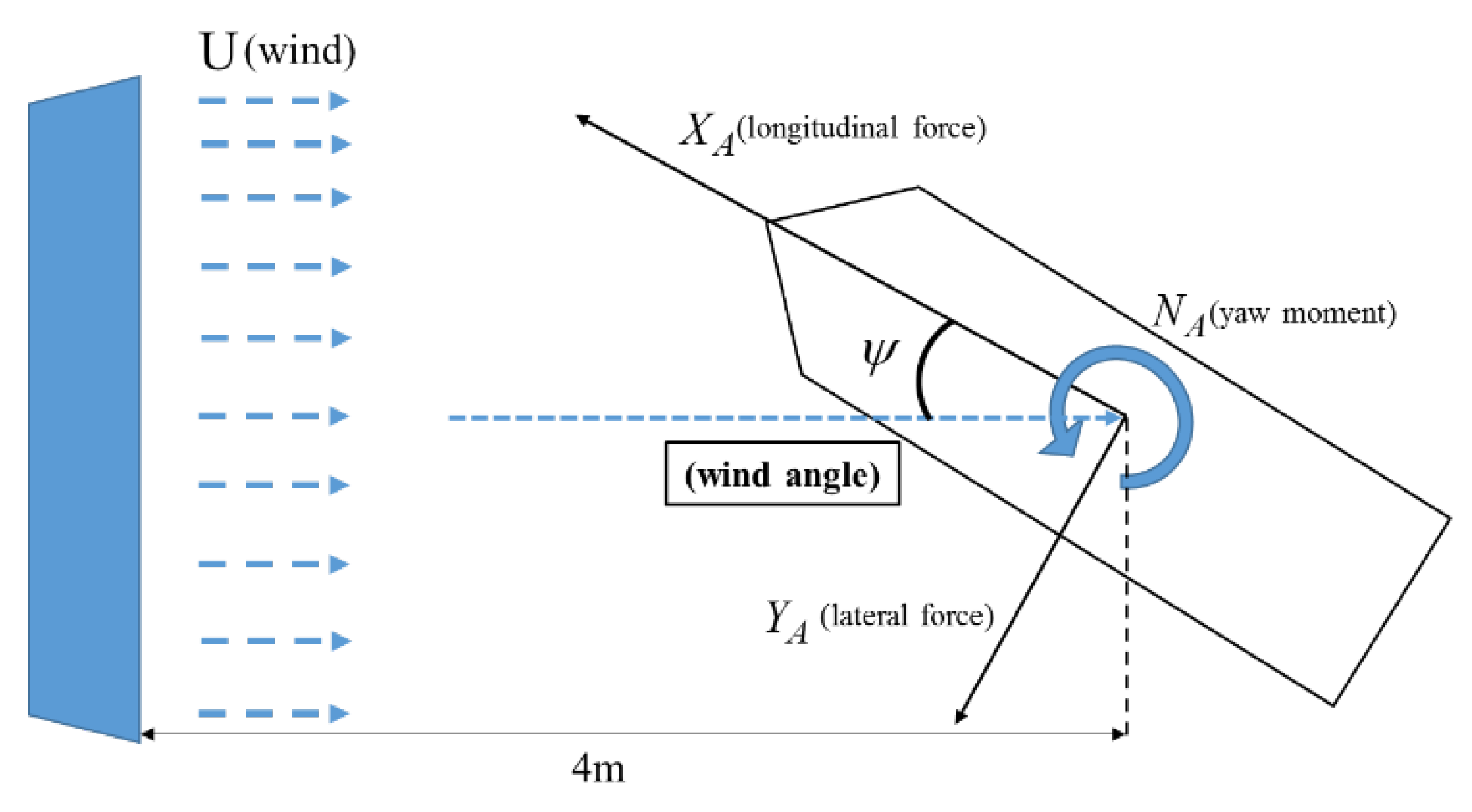
The coordinate system used in this study is the same as that described in the experimental measurement proposed by [19] and is shown in Figure 3.
The wind force coefficients including CX and CY are defined as the following Equations (4) and (5) according to the coordinate system shown in Figure 3, where XA is the longitudinal force, and YA is the lateral force. The yawing moment coefficient CN using the Z-axis is defined as Equation (6). The pressure coefficient and pressure-difference coefficient are defined as Equations (7) and (8), respectively.
As shown in Equations (7) and (8), p, p1, and p2 are the pressures at the point at which the pressure coefficient is being evaluated, while p∞ is the pressure in the free stream.
2.2.3. Mesh Generation
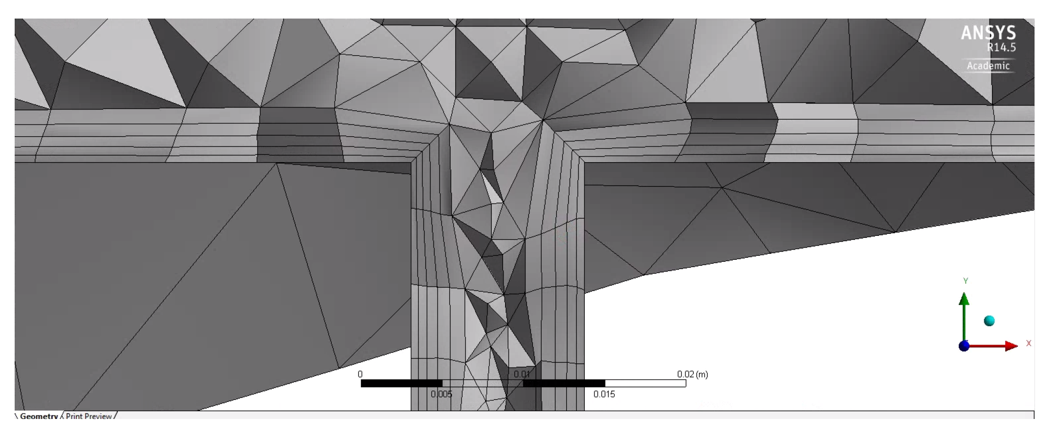
The computational domains are discretized into the mesh cells. Meshing is an important step because the mesh quality significantly affects the computational results. In this study, due to the complexity of the model, the unstructured mesh with a tetrahedral cell is generated for the global mesh; then the mesh refinement is used in the near-wall regions. The mesh independence has been studied in advance [23,24]. The final mesh is approximately 4.6 million cells. The maximum skewness is about 0.866 and the maximum y+ is less than 25 for the refined mesh. The global and local meshes near the model surfaces are shown in Figure 4 and Figure 5, respectively.
2.2.4. Solution Setup
The SIMPLE method is used for steady simulation and the Second Order Upwind scheme is used for the momentum, turbulent kinetic energy, and turbulent dissipation rate. k-epsilon is selected as the turbulence model, while the standard wall function is also applied for the near-wall treatment [25]. It has been confirmed that the k-epsilon model is sufficiently accurate to estimate the performance differences between the superstructures of a container ship in practice [15,16,17]. The velocity inlet and pressure outlet are applied for inlet and outlet boundaries, respectively. To simplify the simulation, the atmospheric boundary layer is not considered. On the ship surfaces, the no-slip condition is considered, while on the top, bottom, and sidewalls of the computational domains, the slip condition is applied. The second-order upwind is selected for the momentum, turbulent kinetic energy, and turbulent dissipation rate to increase the accuracy of the solver. Because it was reported that at high wind speeds, the wind load coefficients are independent of the wind speed and free-stream turbulence intensity [15], in this study, the inflow speed is fixed as 10 m/s. This wind velocity can help maintain the dynamic similarity between the simulation and experiment. The descriptions of the simulation setup and the numerical method are listed in Table 2.
3. Results and Discussions
3.1. CFD Validation
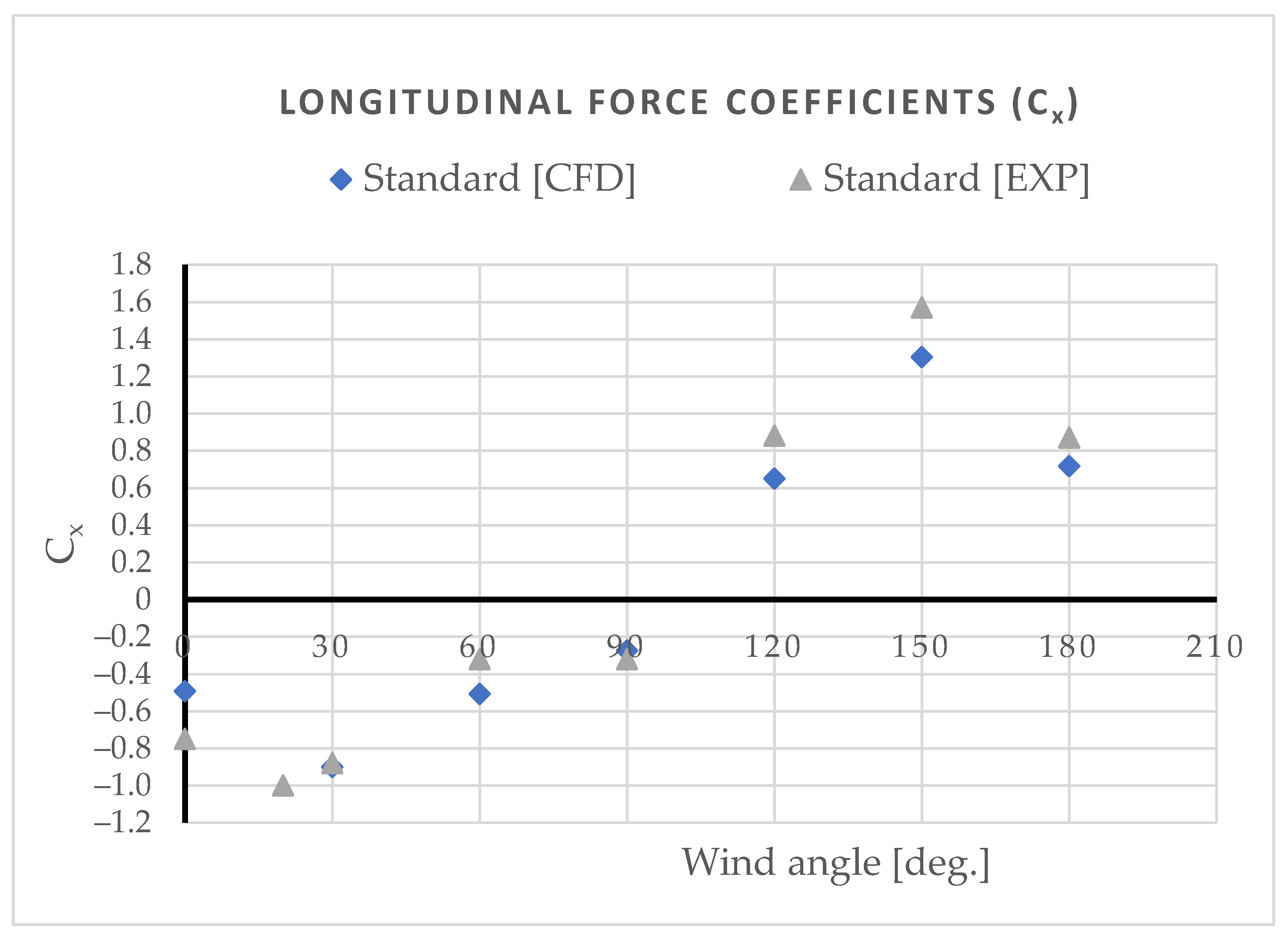
The calculated longitudinal force coefficients acting on the container ship model are compared with those of experimental data reported by Watanabe et al. (Watanabe et al., 2016), as shown in Figure 6.
As shown in Figure 6, the CFD results exhibit the same trend as those of the experimental data; however, the CFD results are slightly underestimated. For instance, the Cx presents negative values for wind angles of less than 120 degrees and positive values for wind angles of higher than 120 deg. At wind angles of between 30 and 90 degrees, the numerical results by the CFD agree well with the experimental data.
3.2. Gap Flow Effects
It was pointed out that the containers loaded onboard ships make the largest contribution (about 80%) to the total air drag. In addition, the air flows passing through the gaps between the containers play an important role in air drag formation (Kim et al., 2015). In this section, the characteristics of the flow passing the gaps between container blocks, engine casing, and accommodation house at the wind direction angle of = 30 degrees are discussed in detail.
3.2.1. Flow in the Gaps between Deck Container Blocks
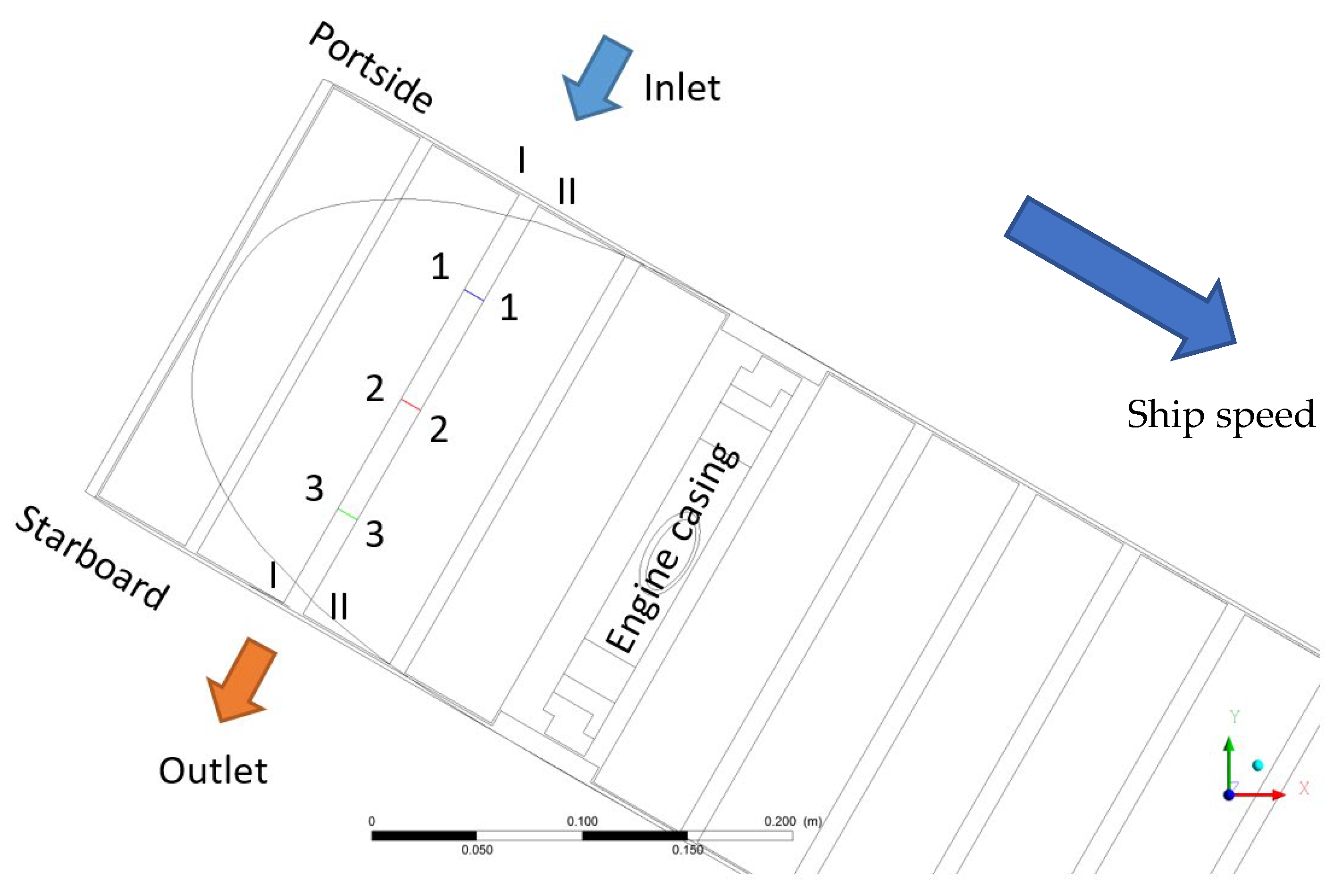
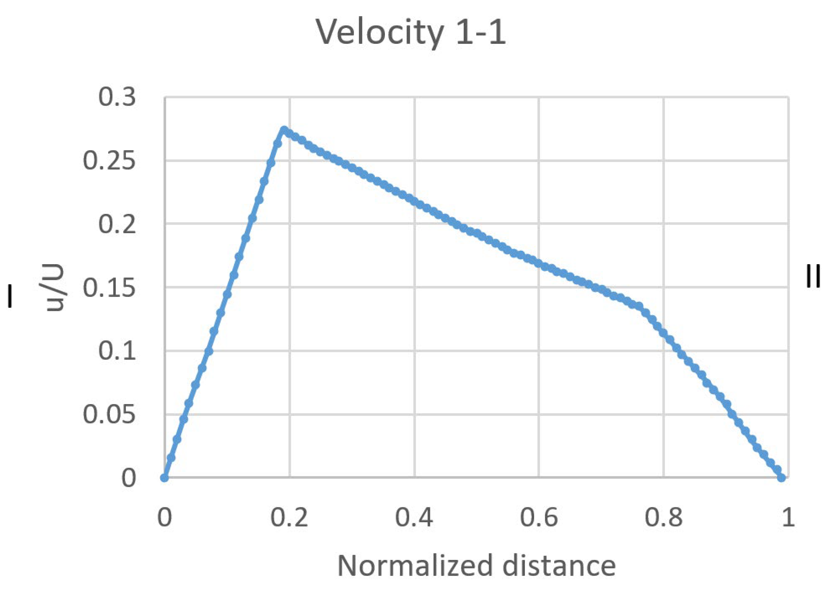
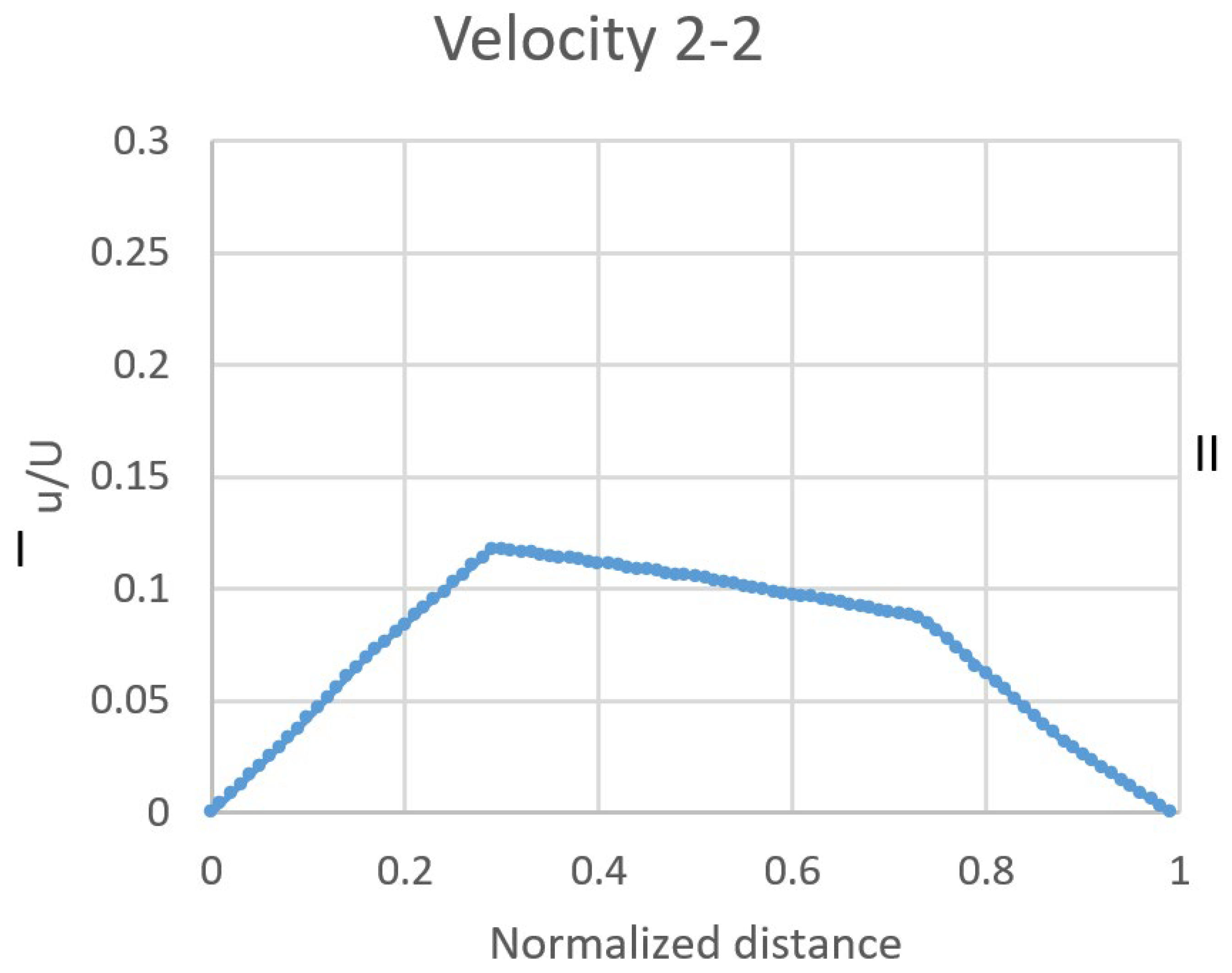
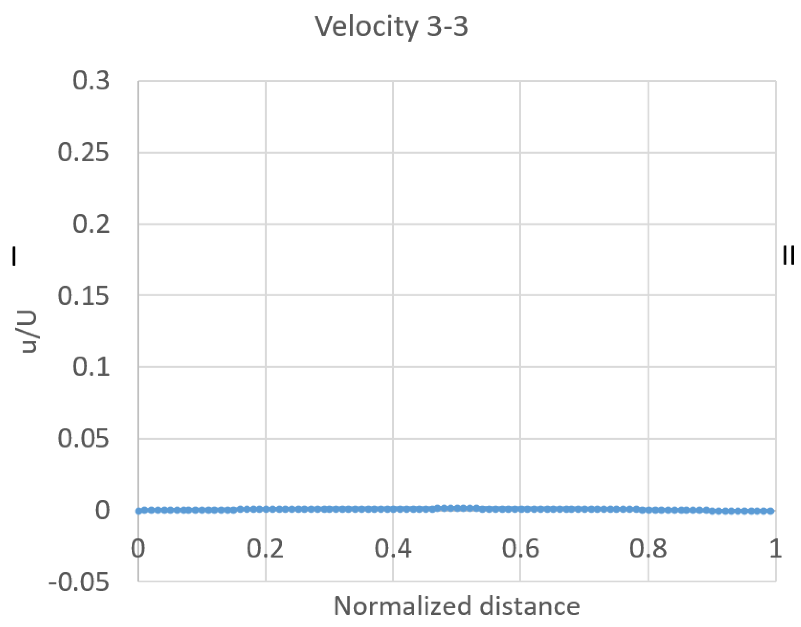
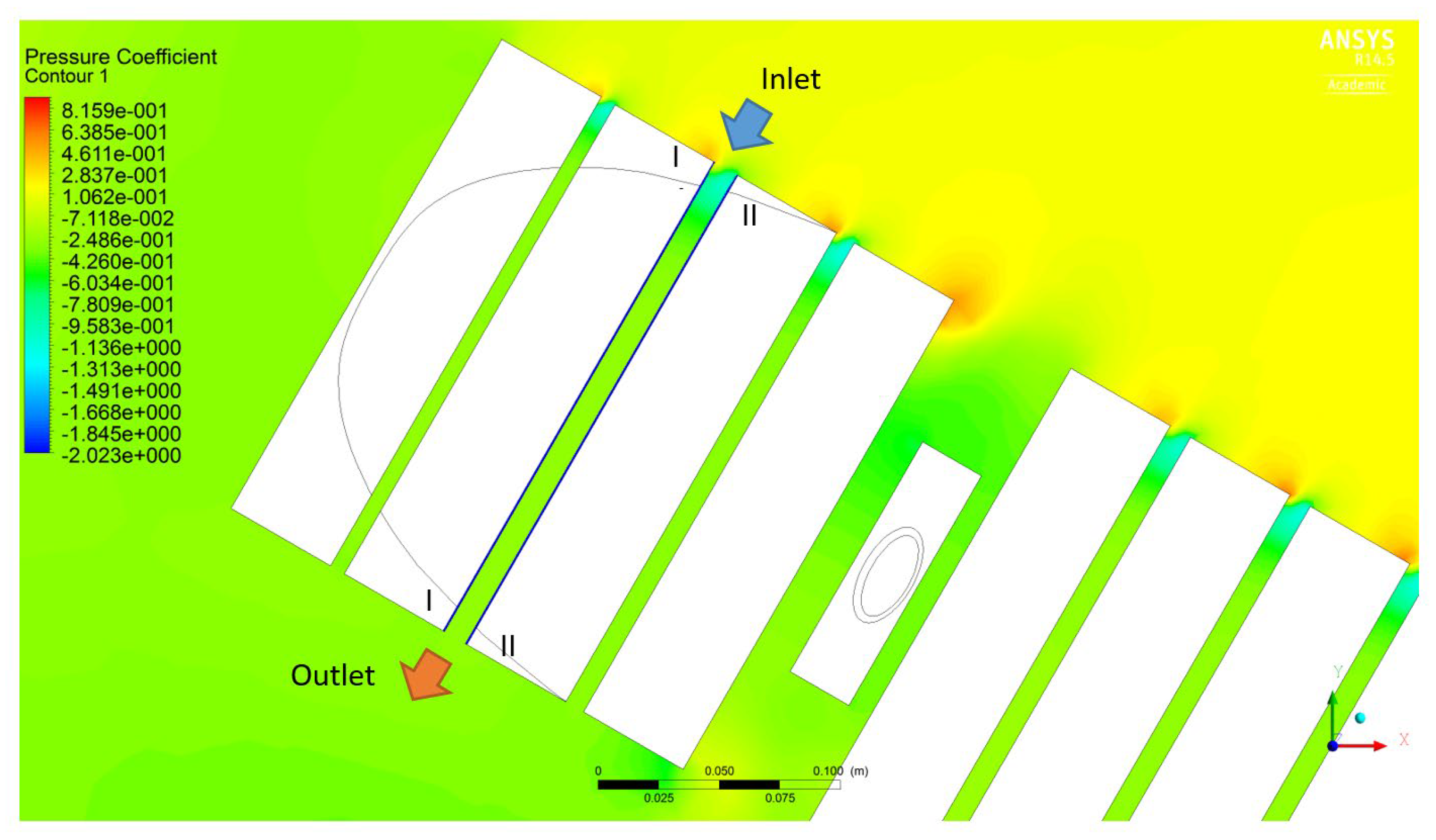
As an example, the flow passing the gap between two parallel walls I-I and II-II at the locations shown in Figure 7 is investigated. The velocity profiles at three positions, upstream (1-1), center (2-2), and downstream (3-3), are shown in Figure 8, Figure 9, and Figure 10, respectively. In these figures, the velocity magnitude, and the distance between the two surfaces of containers are normalized by the outside air velocity and the gap distance between the containers, respectively. Figure 8, Figure 9 and Figure 10 show that the velocity magnitude inside the gap is much smaller than that of the free stream velocity and the velocity values decrease gradually from upstream to downstream of the gap. A double peak exists on the velocity profiles of the upstream (1-1) and center (2-2) sections, while it no longer appears on the velocity profile of the downstream section (3-3) of the gap. For instance, the peak value of the velocity (u⁄U) is about 27% and 12% when the flow passes the gap at the (1-1) and (2-2) sections. It should be noted that, at the downstream cross-section (3-3), the velocity exhibits a very low value and is almost zero. This means that the flow does not horizontally pass through the gap at this cross-section; therefore, a circulation region or reversed flow inside the gap may exist. In other words, no air flow comes out from cross-section (3-3) of the gap at a wind direction angle of = 30 deg.
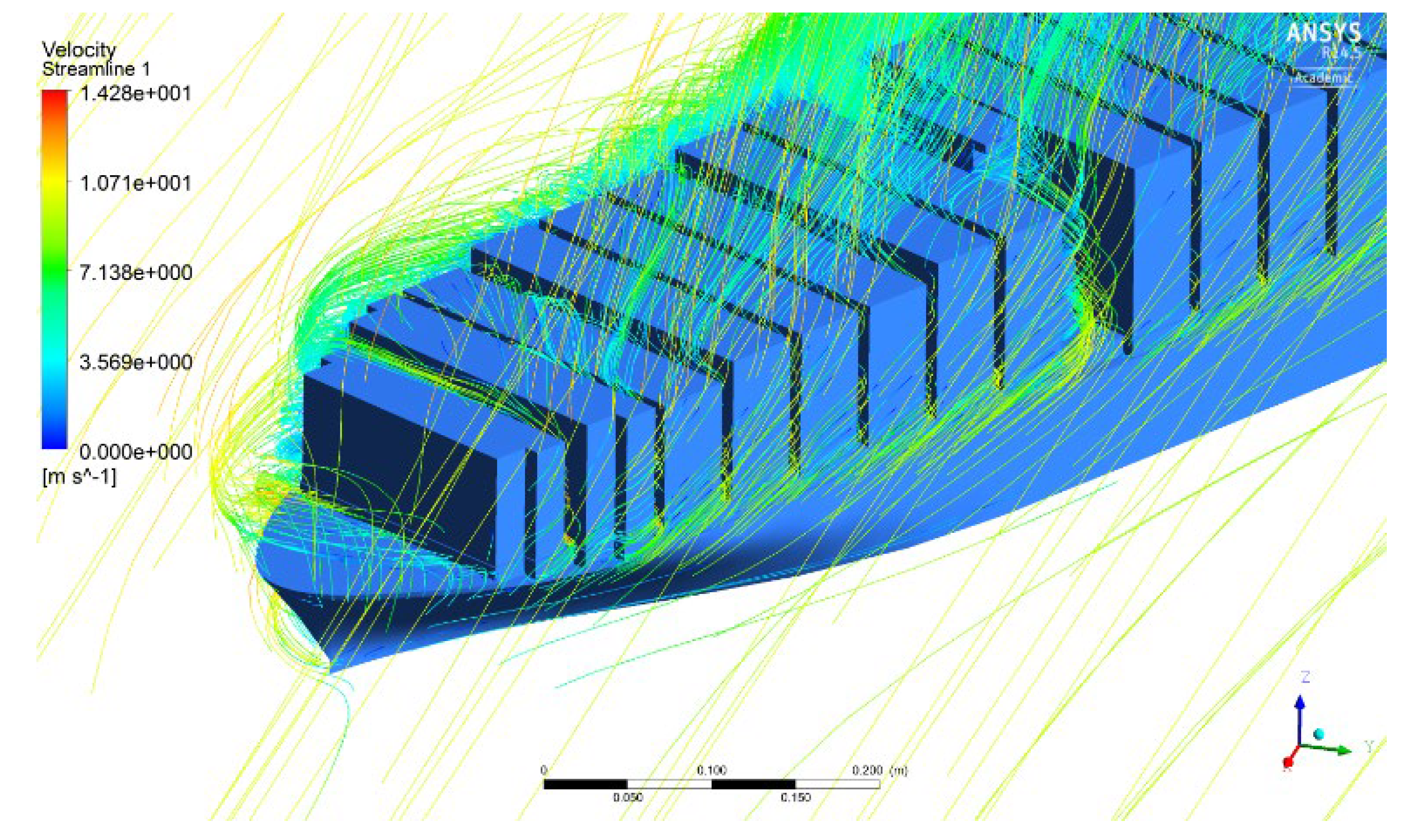
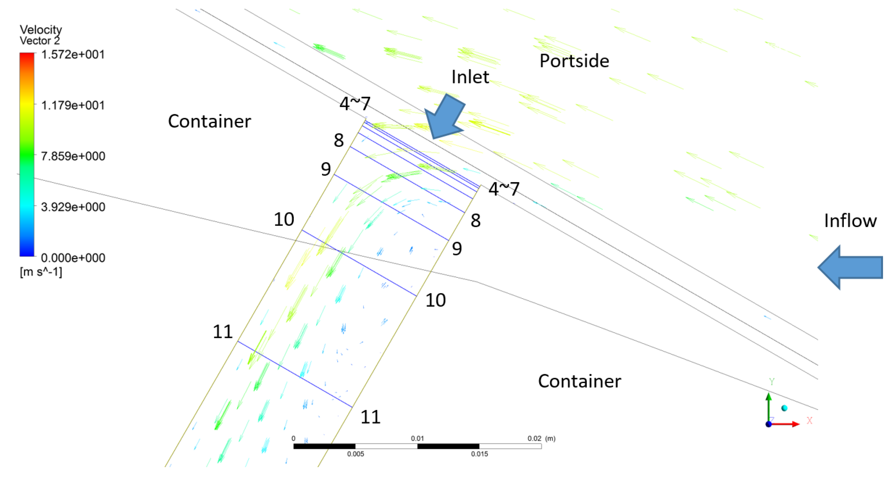
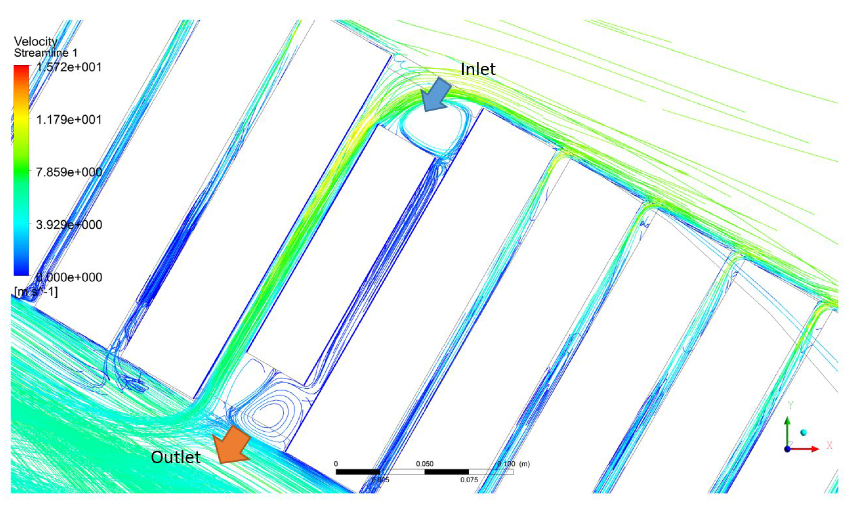
The visualization of flow velocities passing through the gaps is presented in Figure 11 as the velocity streamlines at a wind direction angle of = 30 deg. It can be seen clearly that the flow enters alongside the gaps, then escapes from the top of the container. There is no flow coming out of the gaps at this wind direction angle. This could explain well the velocity characteristics presented in Figure 8, Figure 9 and Figure 10. The distribution of velocity vectors near the gap entrance is shown in Figure 12. As a wind direction angle of 30 degrees, a large separation area occurs near the wall of the front container and occupies about half the breadth of the gap between containers. This is why the velocities near the wall of the upstream container exhibit lower values than the wall of the downstream container, as shown in Figure 8.
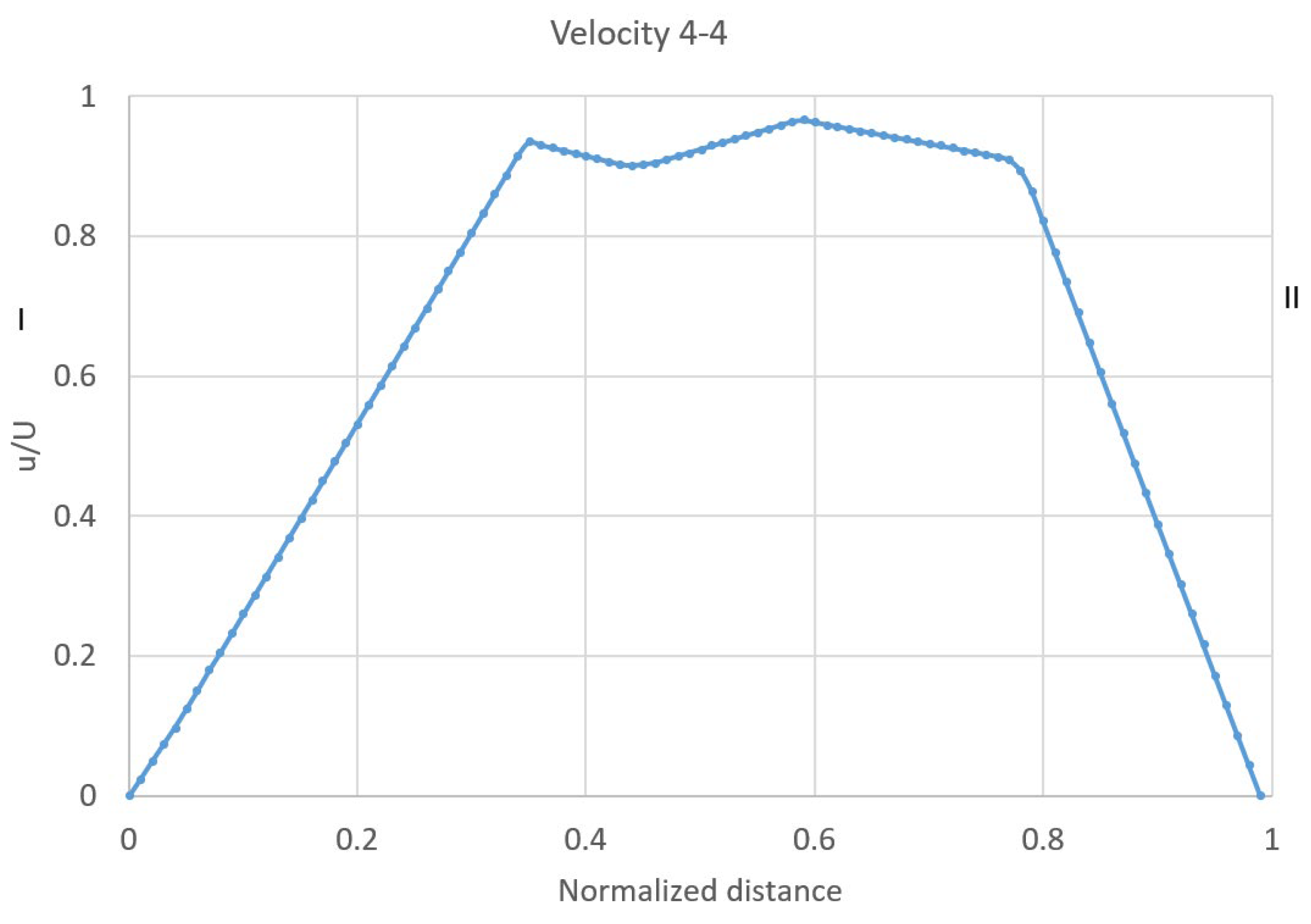
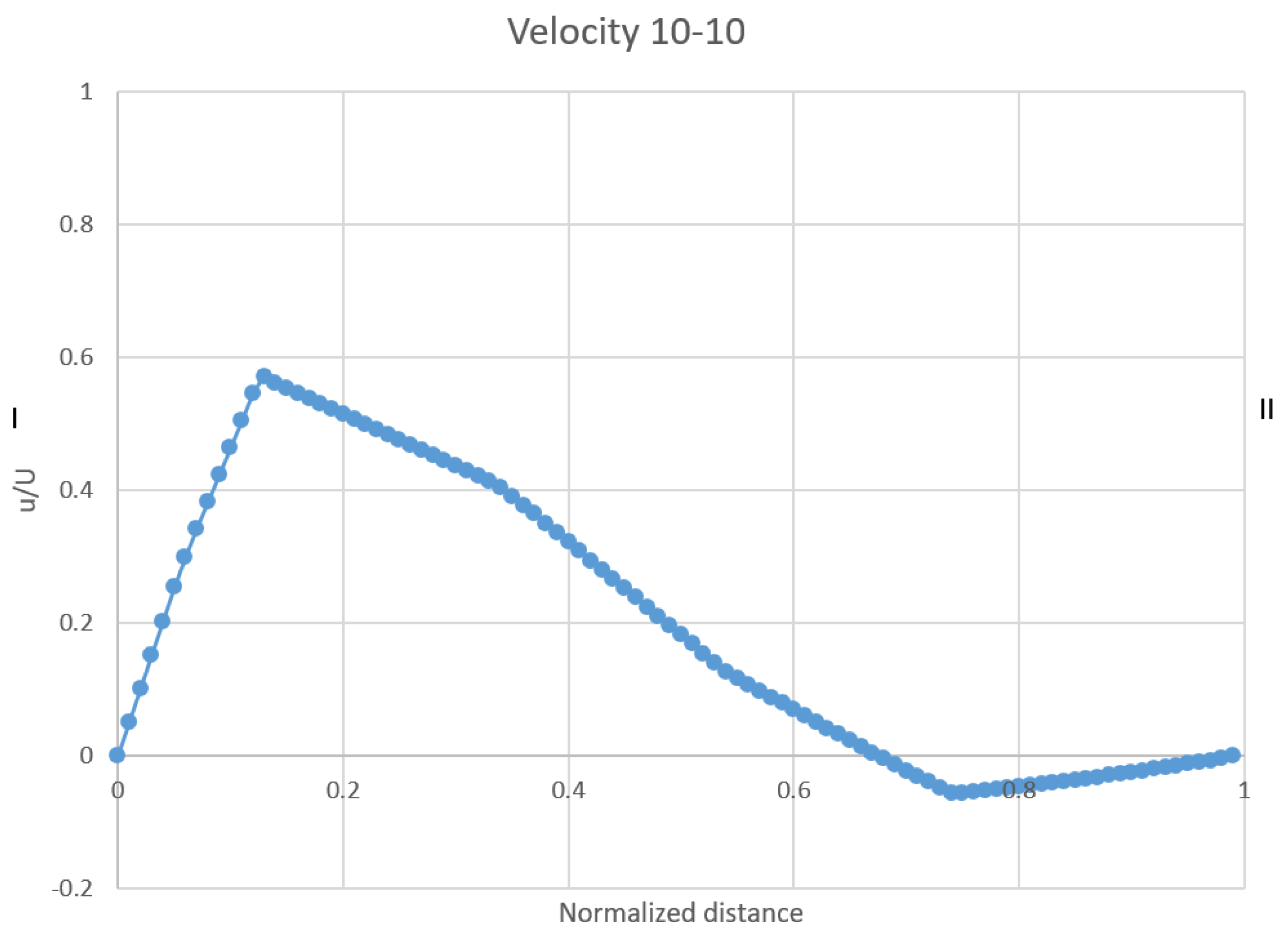
A closer look at the velocity profiles at the two typical cross-sections of (4-4) and (10-10) of the gap, i.e., near the gap entrance, are shown in Figure 13 and Figure 14. As shown in Figure 11, The flow separates at the edge of the upstream container wall before entering into the gap. Therefore, the velocity profile at cross-section (4-4) is very similar to the velocity profile of the flow in a pipe (Figure 13), while the velocity profile at the cross-section (10-10) shows a negative value which corresponded to a reversed flow near the wall of the upstream container (Figure 14).
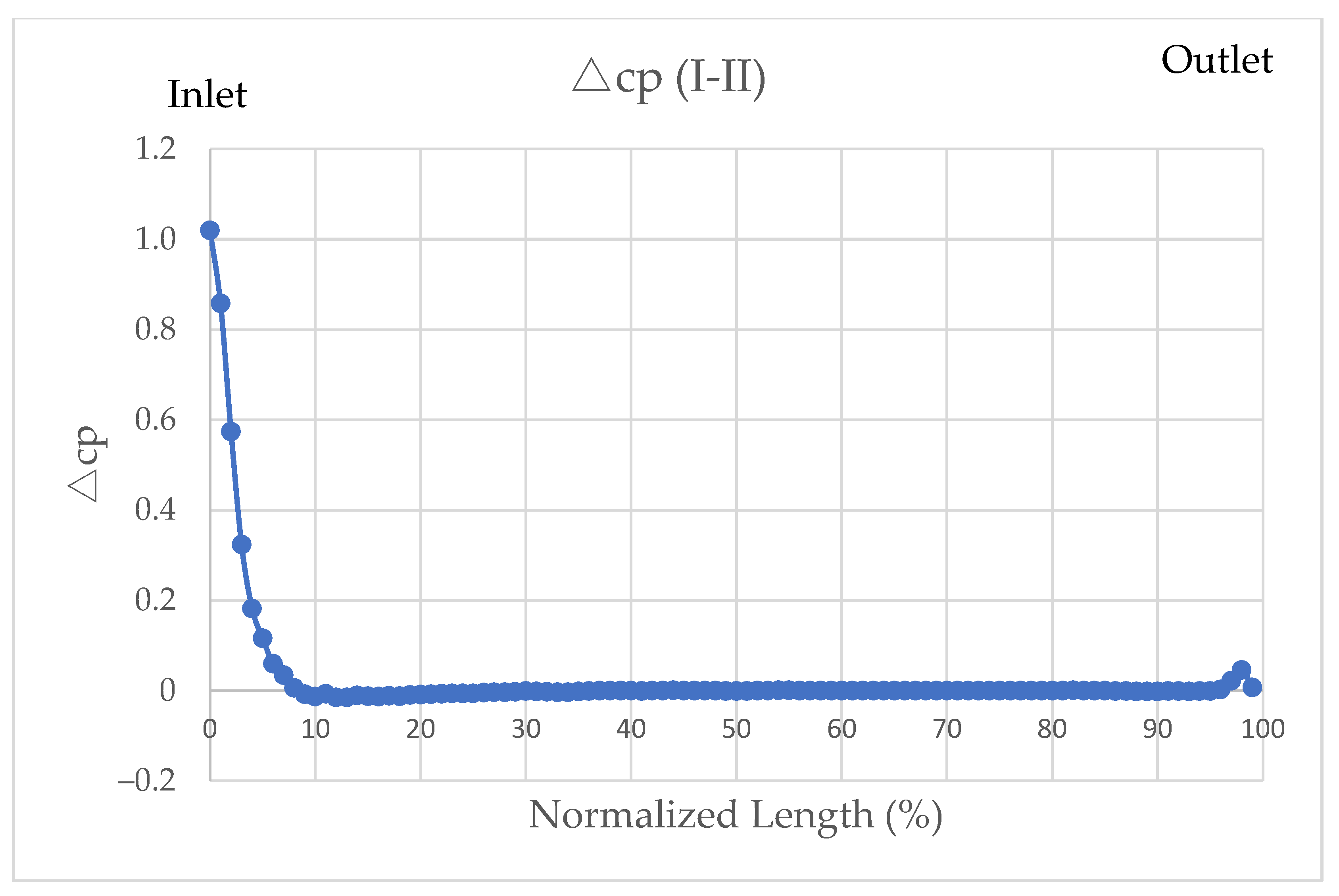
The formation of the vortices induced near the entrance of the gap might indicate the effect of gap air flow on the air resistance of the ship resulting from the pressure distribution. The pressure distribution around containers and the pressure difference coefficients in the gap between the walls (I-I) and (II-II) are shown in Figure 15 and Figure 16, respectively. As shown in Figure 15, high-pressure regions occur at the edge of the entrance of the gaps on the same side as the wind direction, while low-pressure regions exist on the recirculation bubble near the entrance (at about the cross-section (4-4) to (11-11) in Figure 12). Figure 16 shows the pressure difference between the walls of (I-I) and (II-II). The pressure acting on I-I (the frontal surface) is positive while the pressure acting on II-II (the back surface) is negative. At the corner of the frontal surface, a stagnation pressure appears. Therefore, the peak of the pressure comes close to 1. The is significantly high near the inlet (about 0–10% of length), while at the remaining distances, the pressures acting on the front and back walls are almost the same. As the pressure difference exhibits a positive value, it can contribute to the resistance; therefore, this may lead to the increase in air resistance of the ship in the longitudinal direction as the flow goes through the gap between the containers.
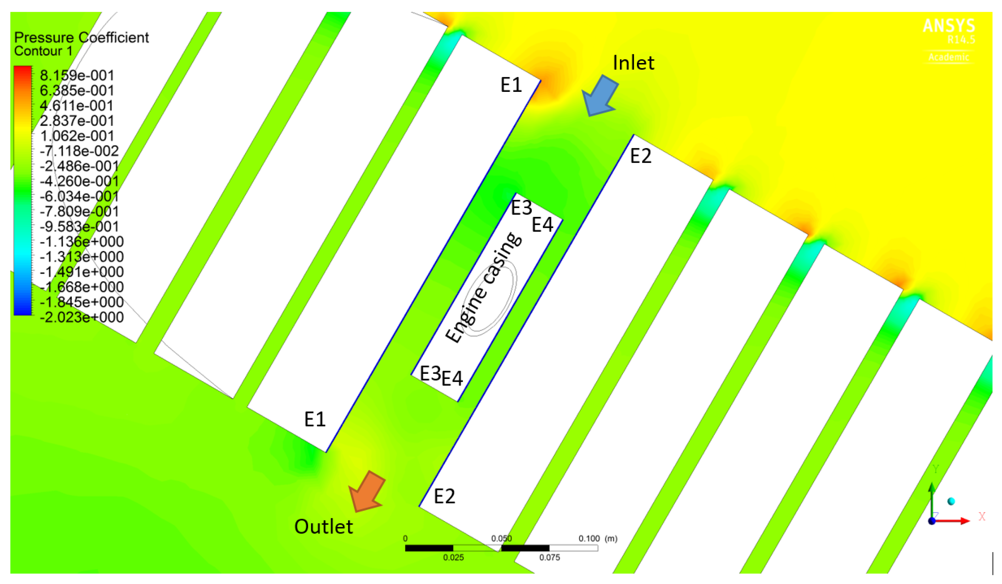
3.2.2. Gap Air Flow at the Engine Casing
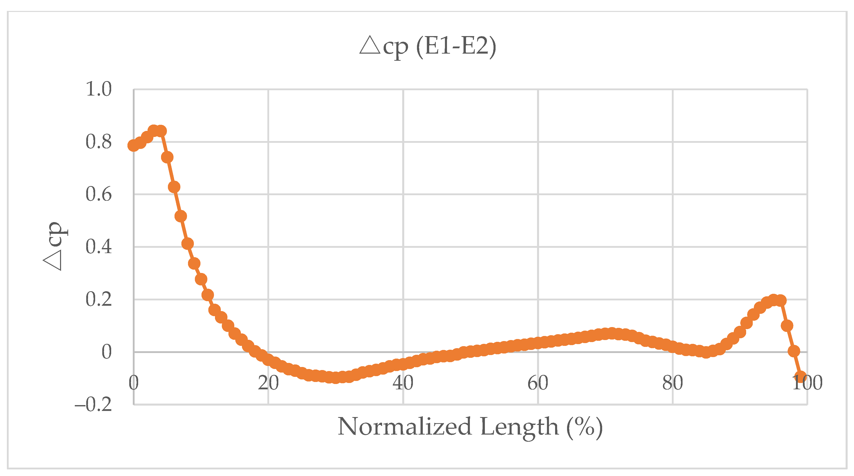
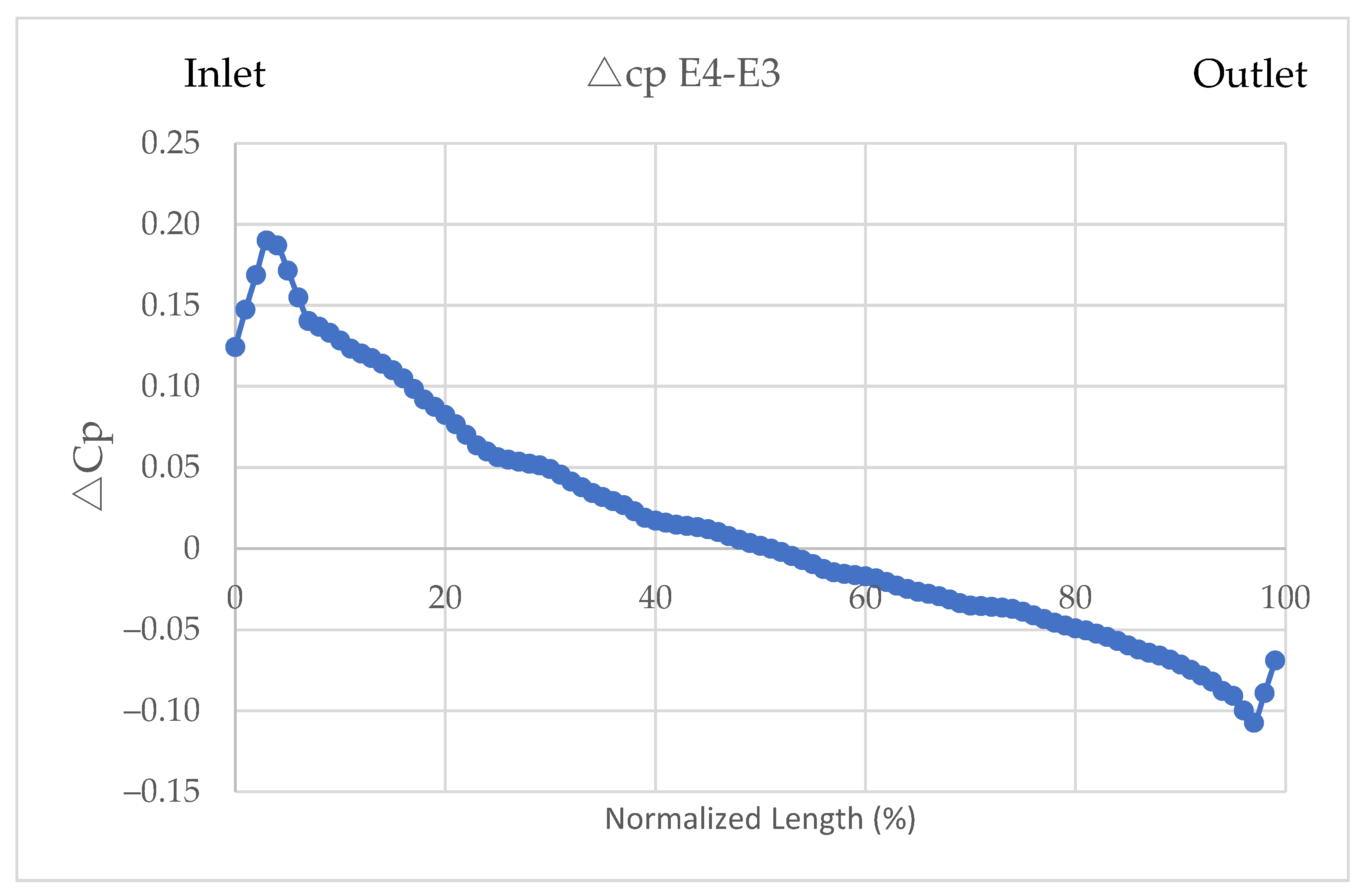
As the gap at the engine casing is larger than the gaps between containers and the engine casing works as an obstacle to air flow in the gap, the air flows passing the gaps between the engine casing and container blocks are investigated carefully. The pressure distribution around the engine casing is shown in Figure 17. The coefficients of the pressure difference between the walls of (E1-E2) and (E4-E3) are presented in Figure 18 and Figure 19. The pressure difference is calculated by subtracting the second surface from the first. For example, the pressure difference between E1-E2 is calculated by subtracting the pressure of the surface E2 from that of the surface E1. Figure 18 shows that the large difference in the pressure acting on E1 and E2 walls occurs at about 0–20% of the length of the gap from the edge of the entrance. The maximum value of is about 82% at the length of 5%. After 20% of the length, the fluctuates within the range of −10% to 20%. The positive values of at near the exit of the gap occurred due to the existence of a high-pressure region. Figure 19 presents the coefficient of the pressure difference between the wall of E4-E4 and the wall of E3-E3 of the engine casing. As shown in Figure 19, the pressure difference between the face and back surfaces of the engine casing exhibits a low value; therefore, only a small resistance is created. For instance, the positive values of occur when the length is less than 50%, e.g., the peak value of is about 19% at a length of 5%. After 50% of the length, the becomes negative.
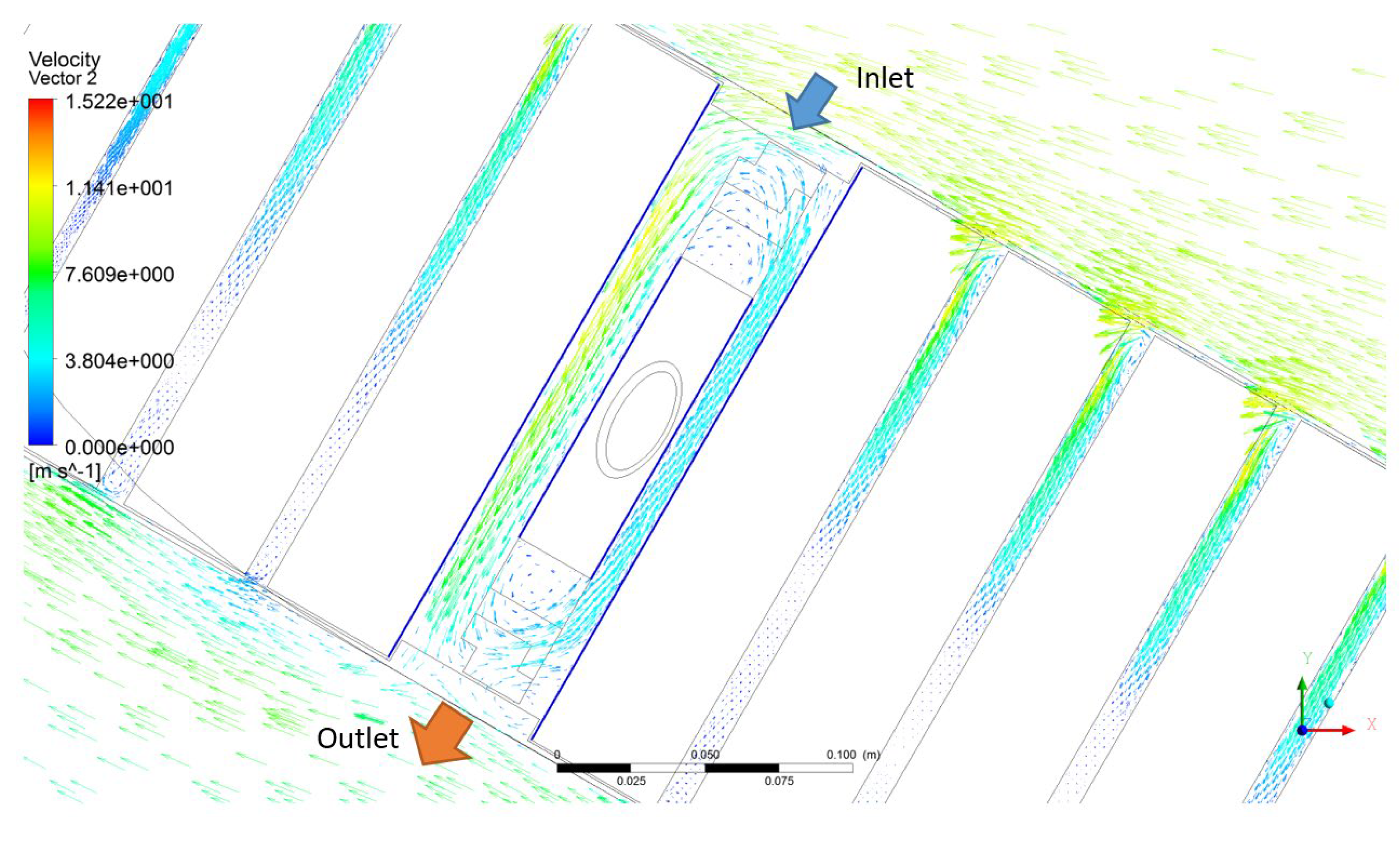
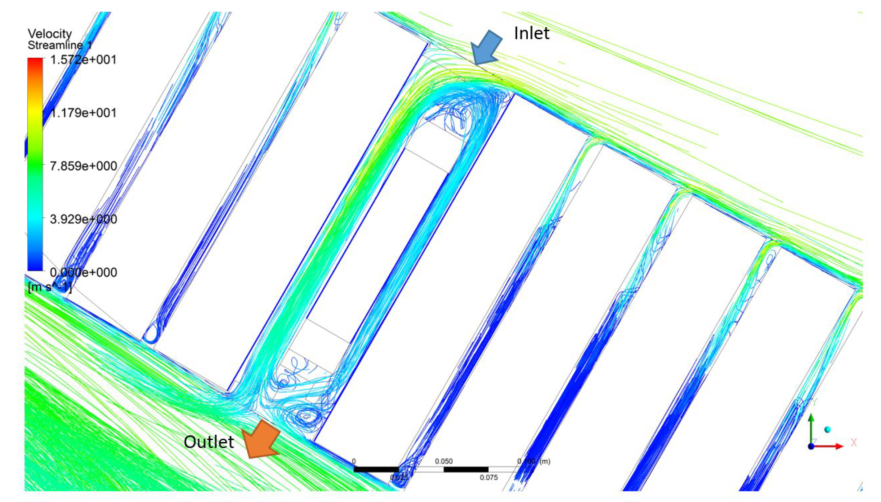
The velocity vectors and the streamlines around the engine casing are revealed in Figure 20 and Figure 21. The large circulation area induced inside the large gap between container blocks due to the flow separation is the same as that shown in Figure 12. High velocity develops on the inlet side of the engine casing channel, while low velocity develops on the outlet side of the gap. As shown in Figure 20, this recirculation bubble encapsulates the engine casing. Therefore, the velocity near the front wall is significantly lower than that near the back wall at a wind direction angle of = 30 degrees. In addition, as shown in Figure 21, two rotating vortices are induced near the outlet and inlet regions of the gap due to the effects of flow over a bluff body (i.e., the engine casing). Another vortex is found at the outlet of the gap due to the flow separation occurring at the edge of the front container wall.
3.2.3. Gap Flow at the Accommodation House
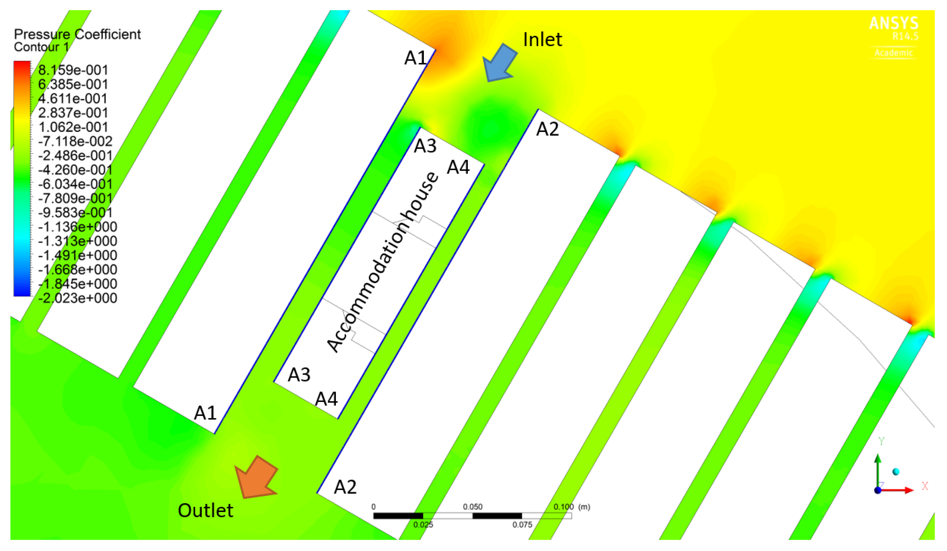
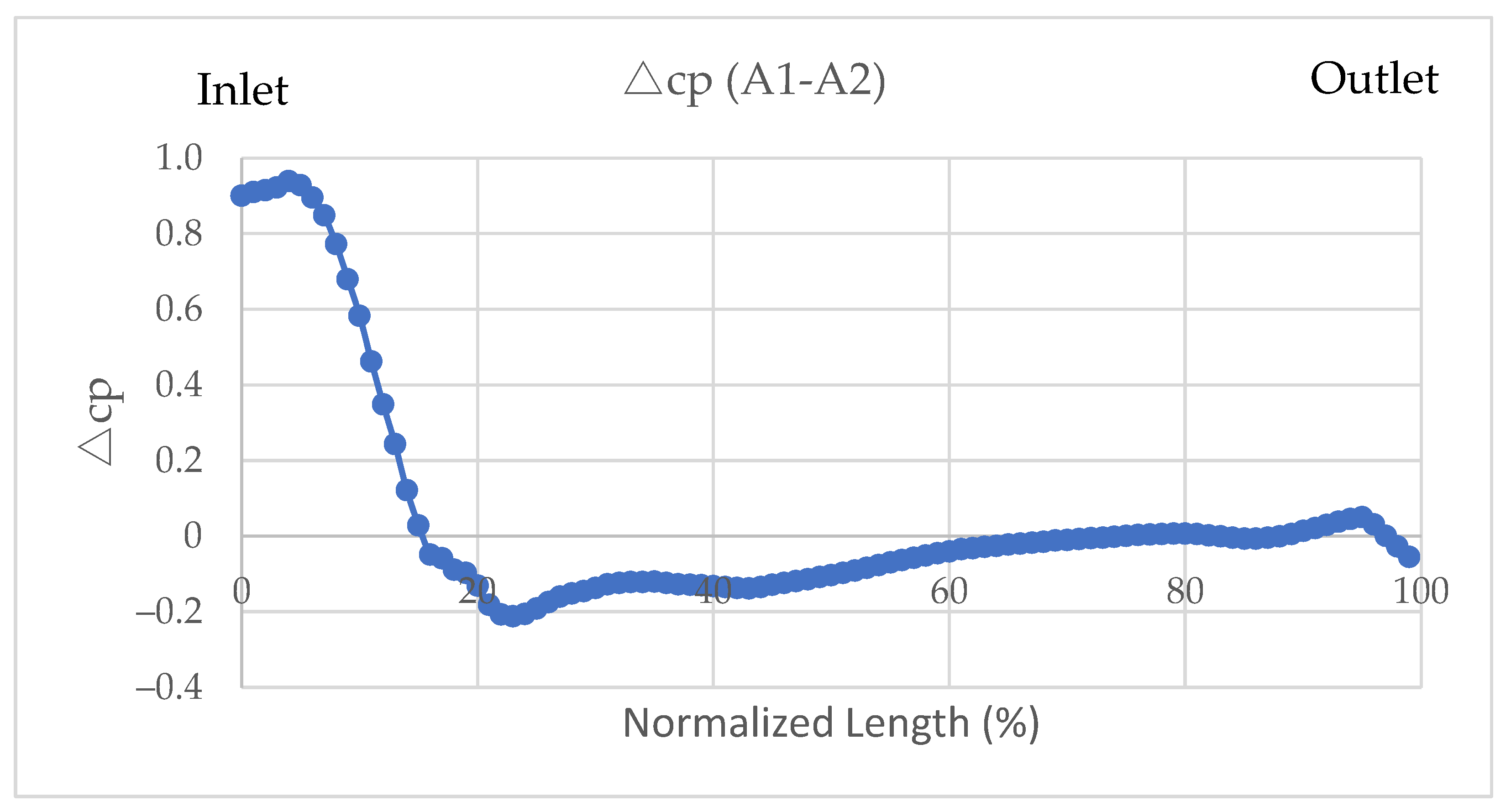
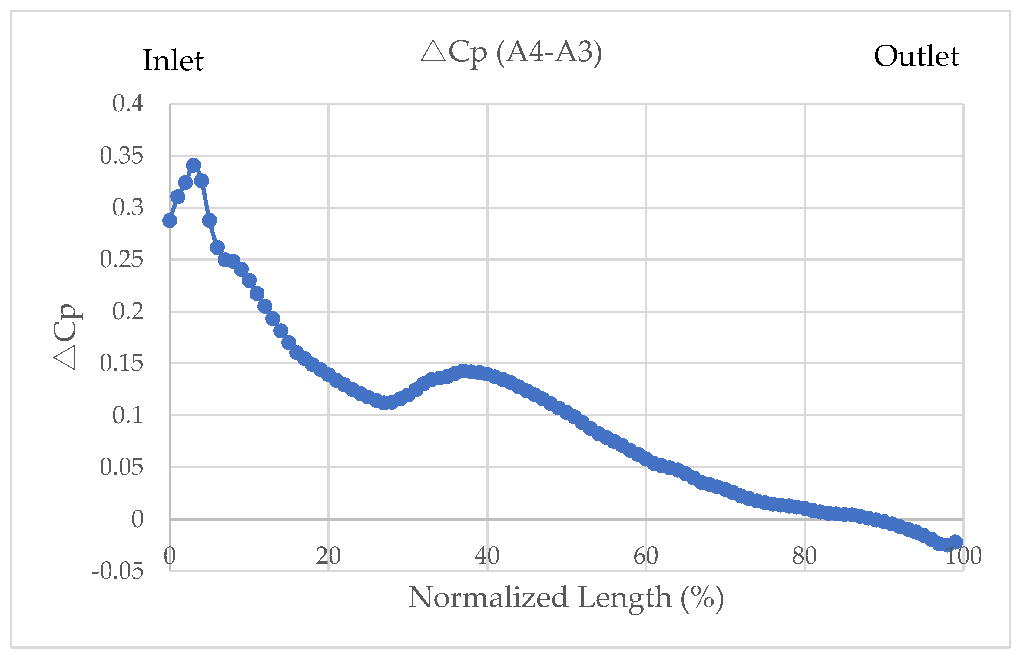
As with the gap air flow at the engine casing, the air flows passing the gaps between the accommodation house and container blocks are investigated numerically. The pressure coefficient distributions of gap air flow around the accommodation house and containers are shown in Figure 22. As shown in Figure 22, a high-pressure region develops at the leading edge of the container block located behind the house (i.e., the A1-A1 wall), while a low-pressure zone develops near the edges of A2, A3, and A4 on the inlet side. The coefficients of the pressure difference between the A1-A2 and A4-A3 walls are shown in Figure 23 and Figure 24, respectively. Figure 23 shows that the largest difference in pressure occurred at about 0–15% length of the gap. For instance, the peak value of pressure is about 95% at 7% of the gap length. At normalized lengths of the gap greater than 7%, the value of rapidly decreases. Beyond 15% of the gap length, the value is negative and slightly increases to about zero. This difference in pressure between the A1 and A2 walls results in a consequential increase in air resistance. Figure 24 shows the difference in pressure acting on the front wall and back wall of the accommodation house. It is clear that a positive value of pressure acts on the house and contributes to the increase in air resistance. For instance, a positive value of pressure is exhibited for a wide range of normalized lengths of the gap (i.e., 0 to 90%). The peak value of is found at 5% of the gap length, while gradually decreasing with increasing gap length.
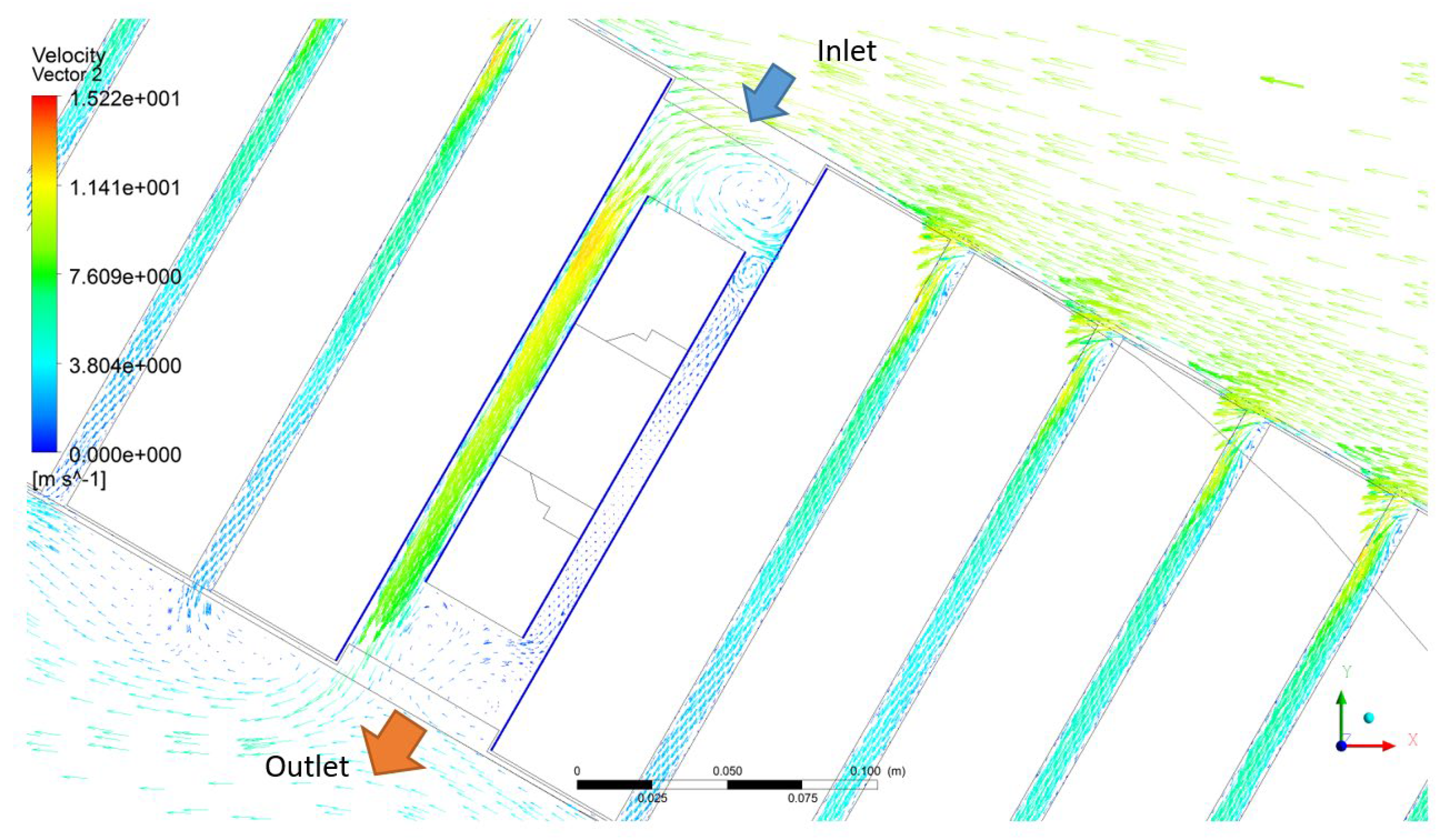
Detailed explanations of the velocity vectors and streamlines around the accommodation house are presented in Figure 25 and Figure 26, respectively. As discussed in Figure 20 and Figure 21, the same trends are found in Figure 25 and Figure 26. For instance, rotating vortices are induced near the inlet and outlet of the gap. The flow velocities in the gap between the back wall of the house and the container wall are significantly greater than those in the gap between the front wall of the house and the container wall due to the flow separation and bluff-body effects.
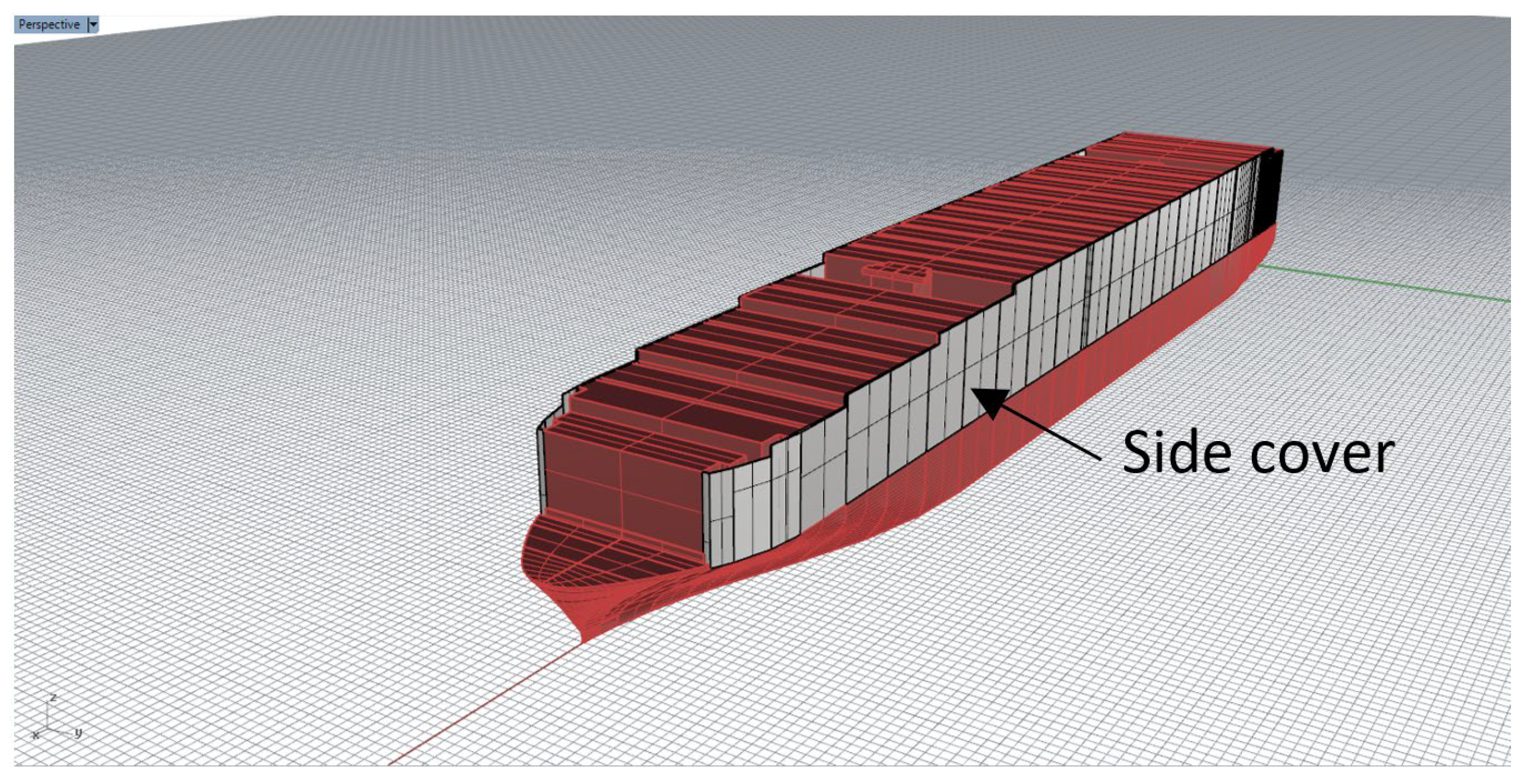
3.3. Shutdown of Gap Flow with Side Cover
As shown in the previous section, the gap air flows among the deck containers play an important role in the air resistance acting on a large container ship. The flows around the model with side covers are calculated in this section. The ship model with side covers is shown in Figure 27.
3.3.1. Pressure and Velocity Distribution at = 30 deg
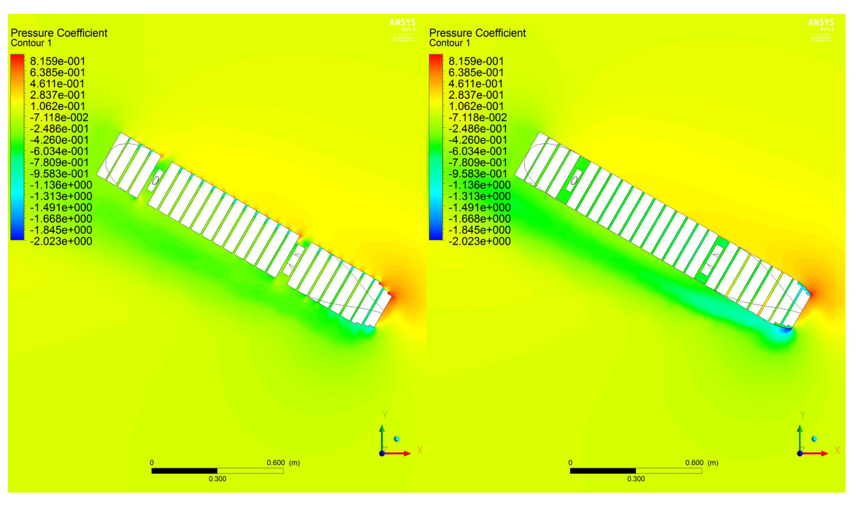
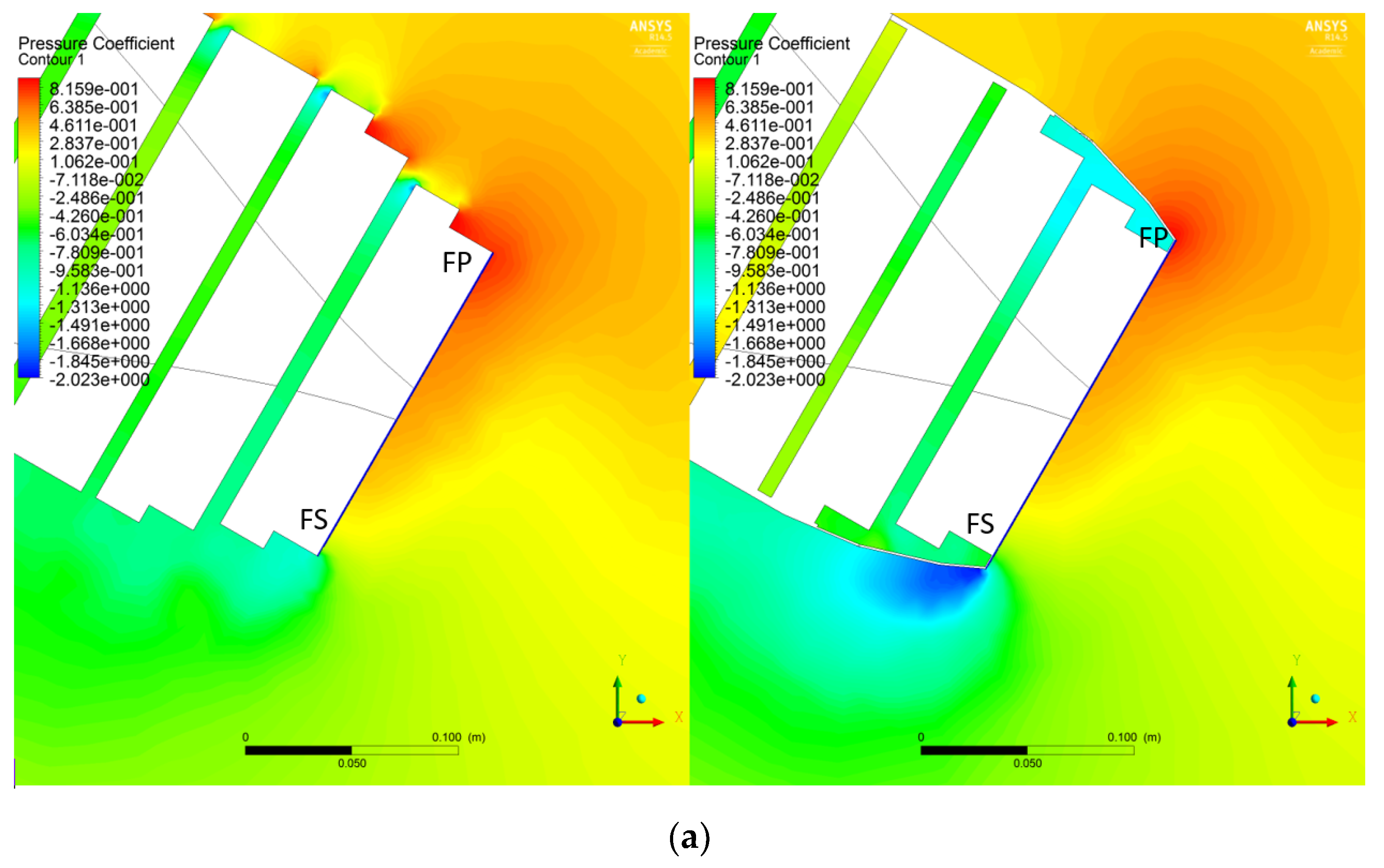
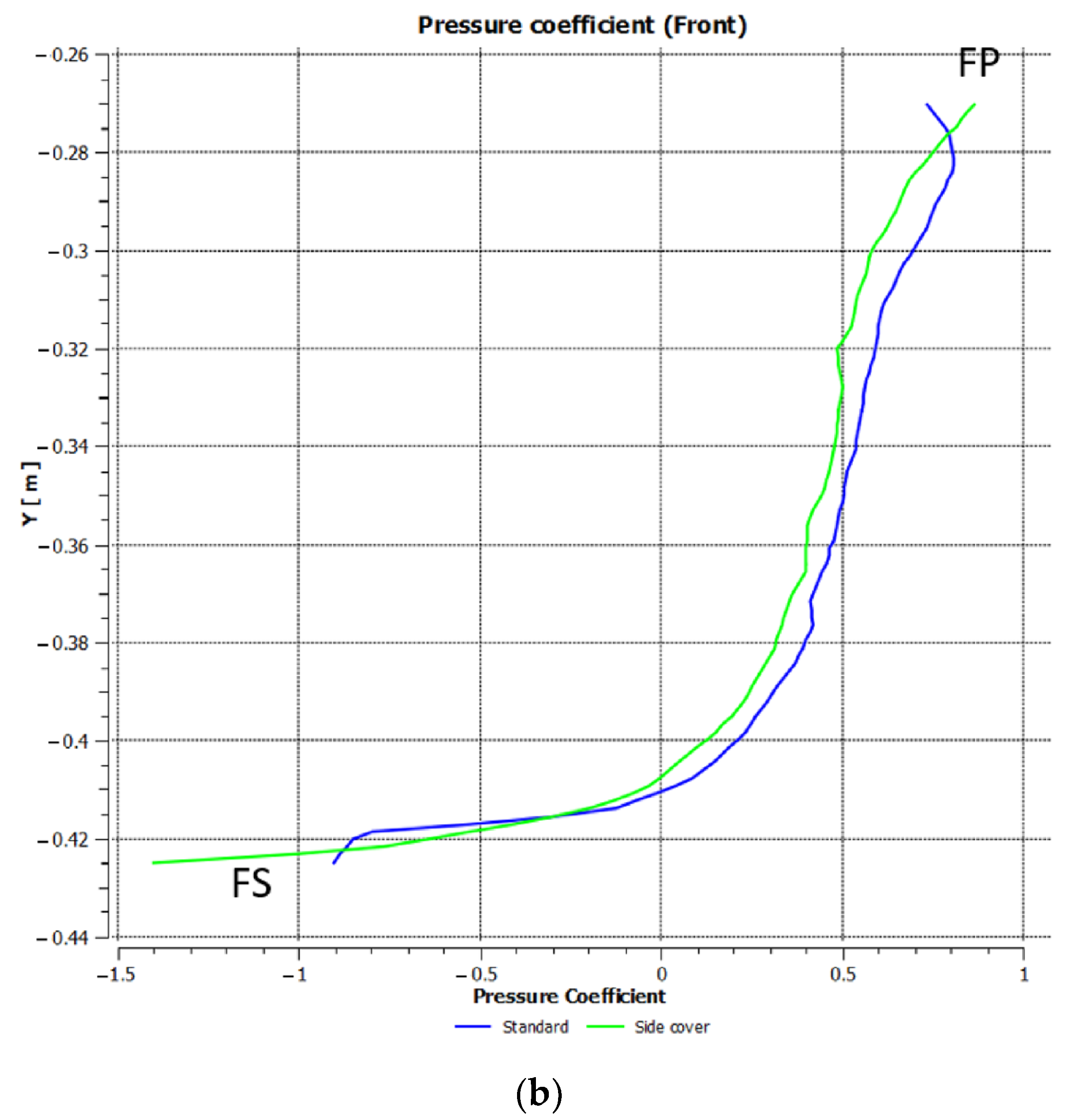
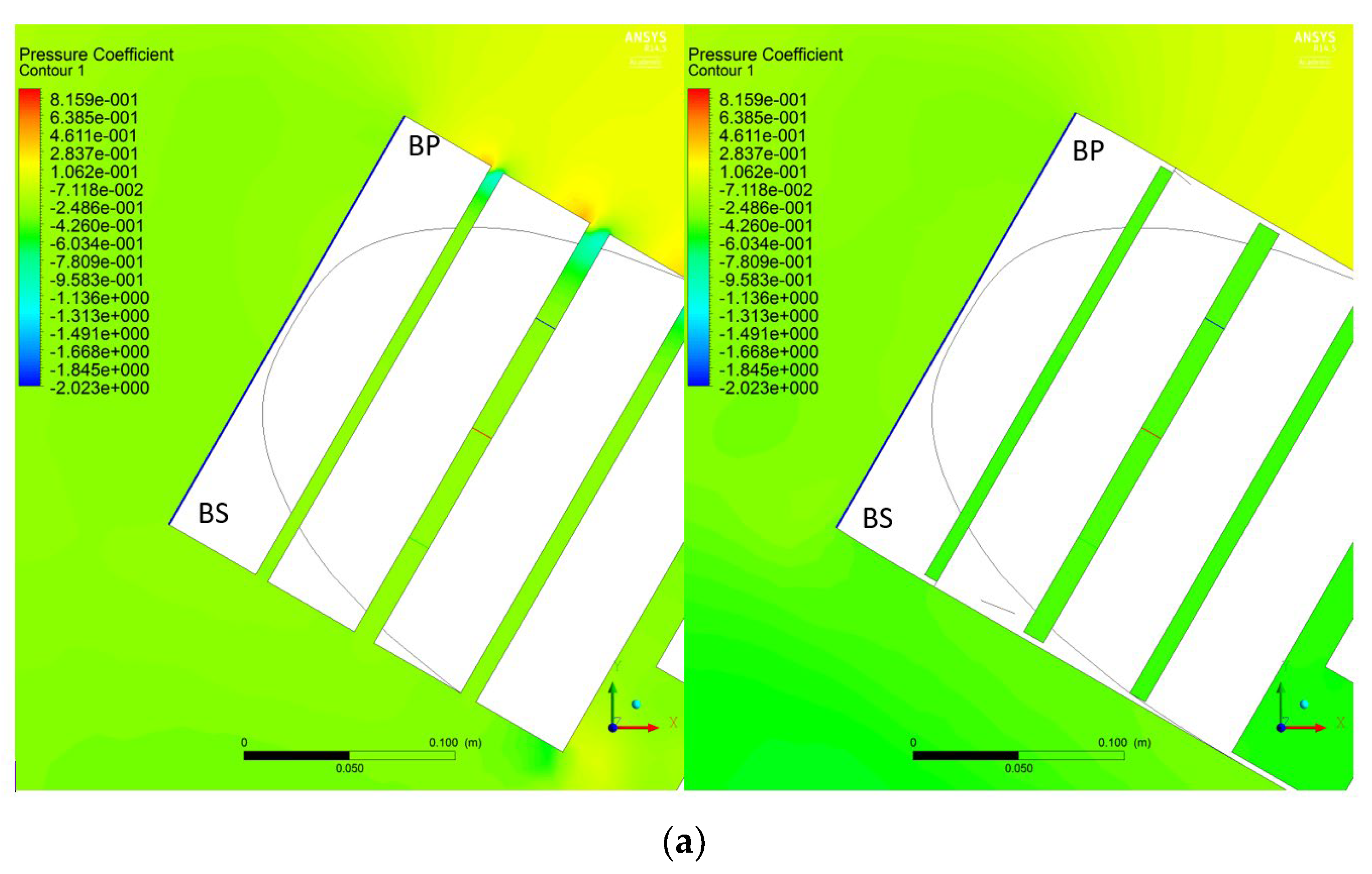
The pressure and velocity magnitude distributions as well as velocity vectors and streamline at z = 0.12 m and 30-degree wind angle are shown in Figure 28, Figure 29, Figure 30, Figure 31, Figure 32 and Figure 33, respectively. In Figure 28, Figure 29, Figure 30, Figure 31, Figure 32 and Figure 33, the left figures present the pressure distribution of the standard model without the side covers, while the right figures present that for the model with the side covers. Figure 29a,b show the pressure distributions on the frontal surface (FP-FS) of the deck containers without and with the side covers, respectively. As shown in Figure 29a,b, the pressure distributions are completely different between the standard model and the model with side covers. For instance, the pressure acting on the face side (i.e., the front port side) of the standard model exhibits large values at the corners of container blocks, while the high pressures are concentrated on a large region at the frontal surface using the side covers. In addition, the pressure coefficient values around the Front-Starboard in the case with the side covers are significantly lower than those in the case without the side covers.
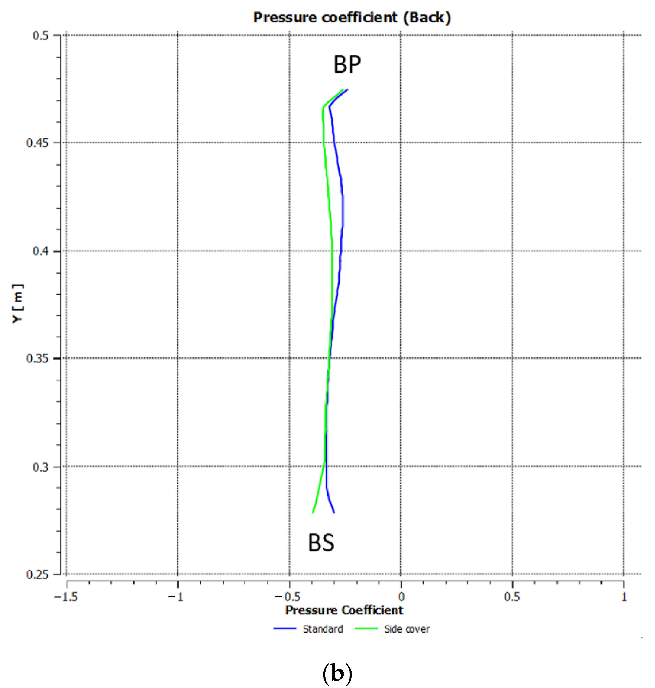
The pressure distributions on the back surface (BP-BS) of the deck containers without and with the side covers are shown in Figure 30a,b, respectively. It can be seen in these figures that the high-pressure region acts on the BP side and the low-pressure region acts on the BS side of the ship models both without and with the side covers. As shown in Figure 29b, there is not much difference in pressure coefficient between the BP and BS sides. In other words, the side covers have only a small effect on the pressure acting on the BP and BS sides, and therefore, most of the contributions to the air resistance are caused by the pressure increase created at the gap entrance of each container block.
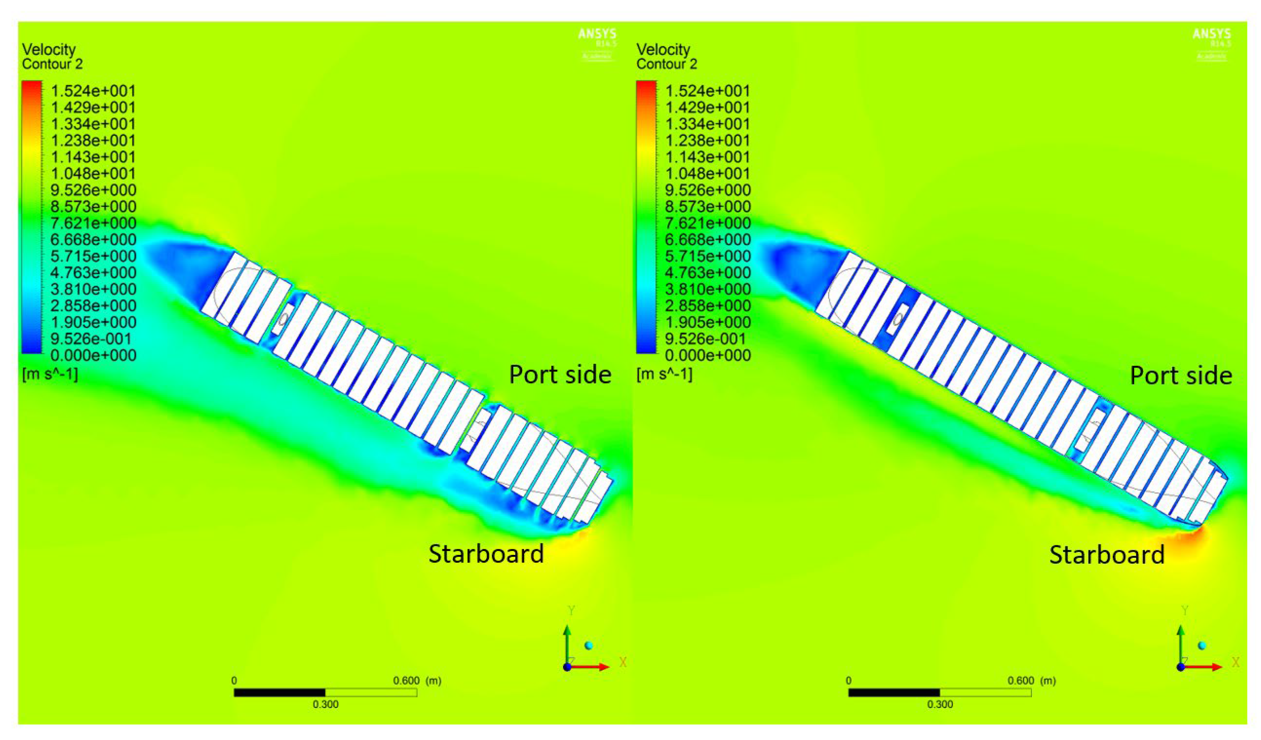
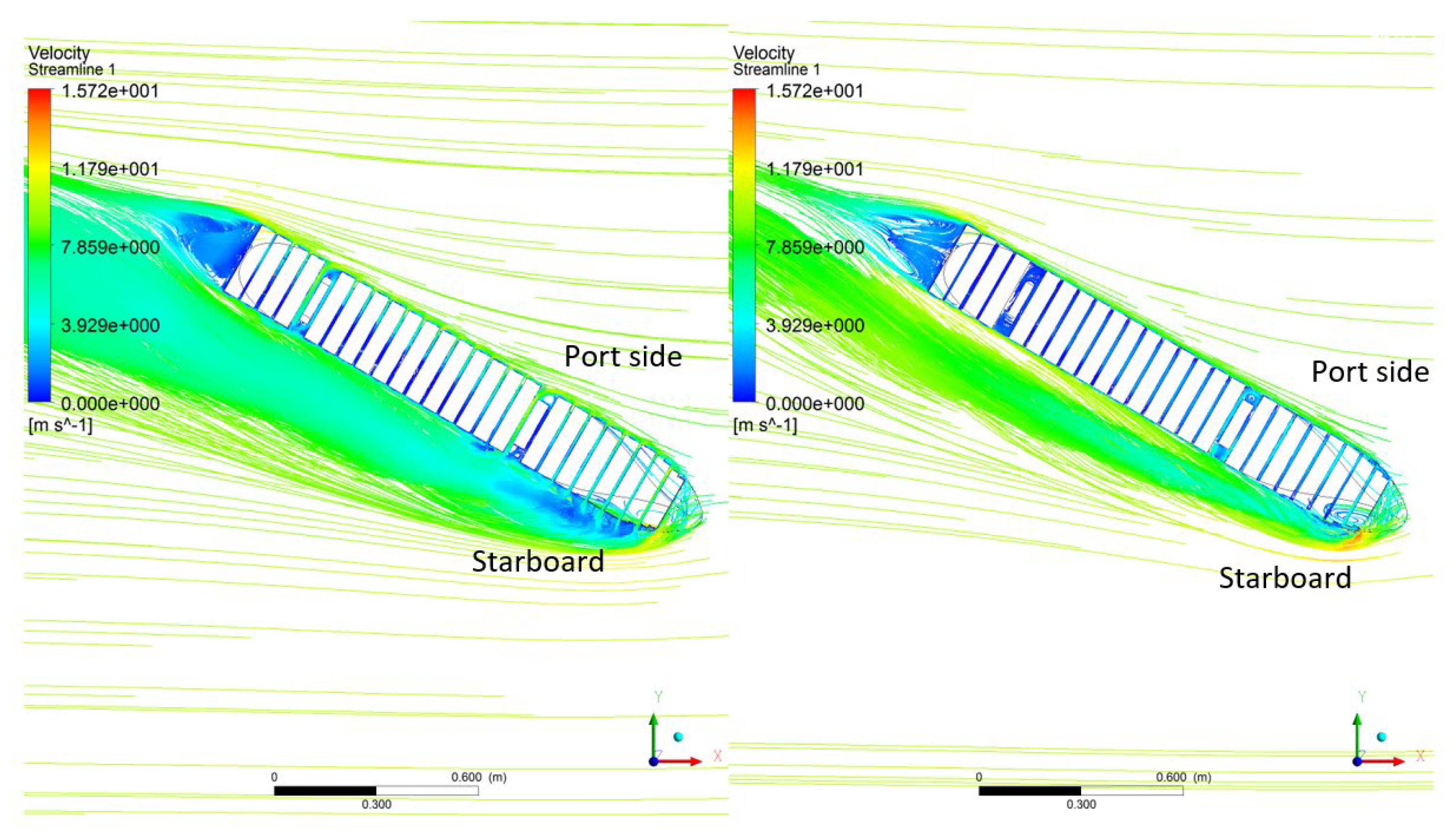
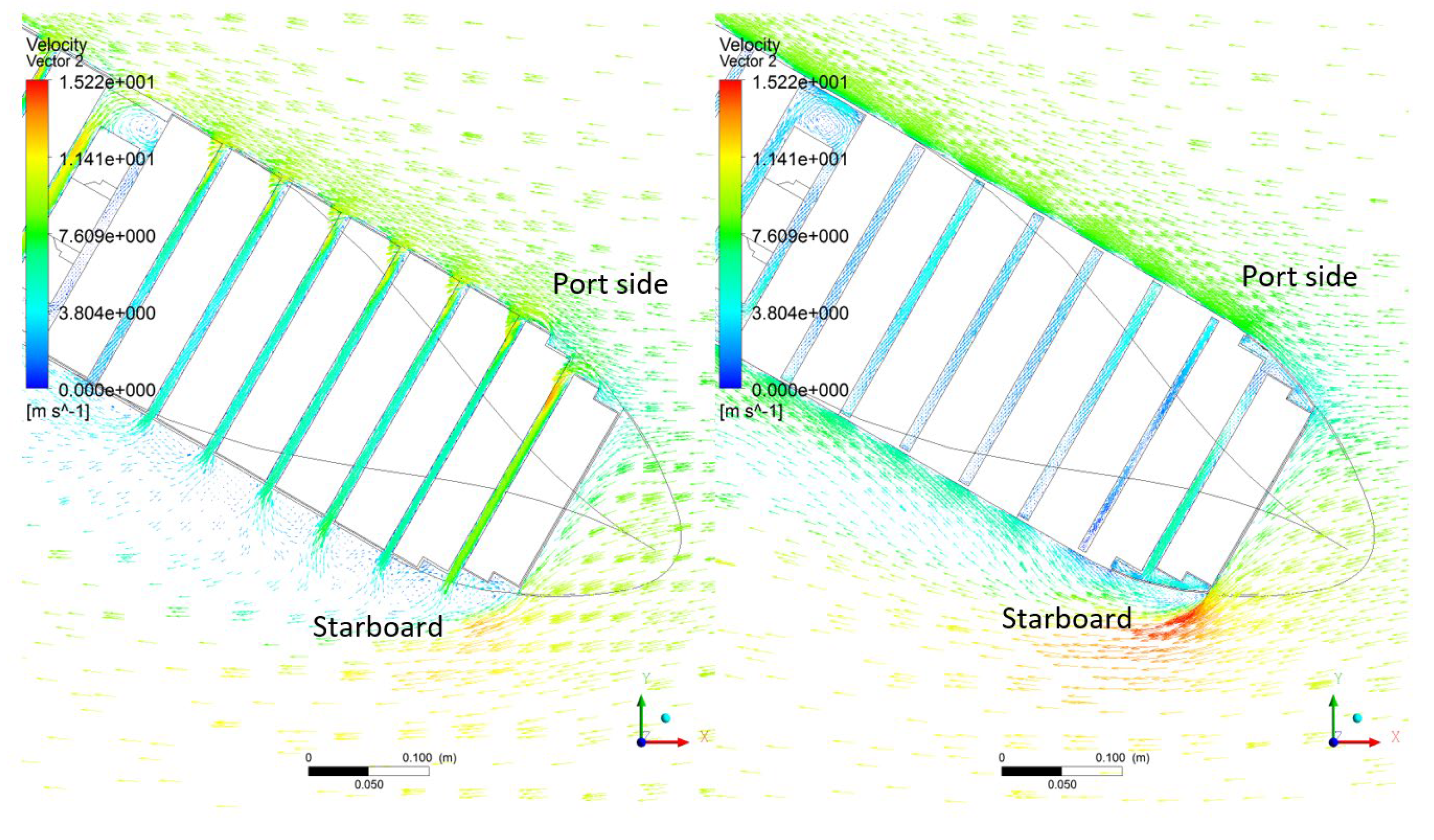
The velocity distributions, streamlines, and velocity vector fields at z = 0.12 m, and = 30 degrees are shown in Figure 31, Figure 32, and Figure 33, respectively. The wakes induced at the starboard side of the model present lower velocity than that on the port side both with and without the side covers. However, a larger wake region occurs using the model without the side covers than with the side covers. This is because every single gap induced between the containers without side covers produces a flow inside a channel, and consequently, each outlet flow creates a wake (Figure 32 and Figure 33). In addition, a low-velocity region is induced in the wake of the ship as the flow passes through a bluff body. The velocities displayed in the model with the cover sides are significantly greater than those in the model without the cover sides, especially near the starboard.
3.3.2. Air Resistance Coefficient
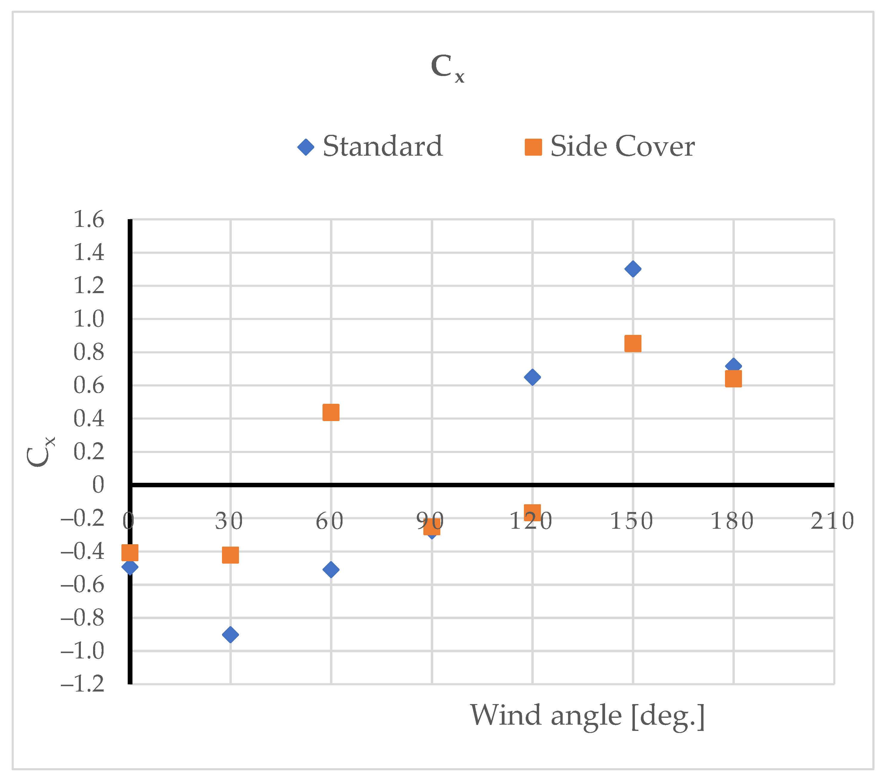
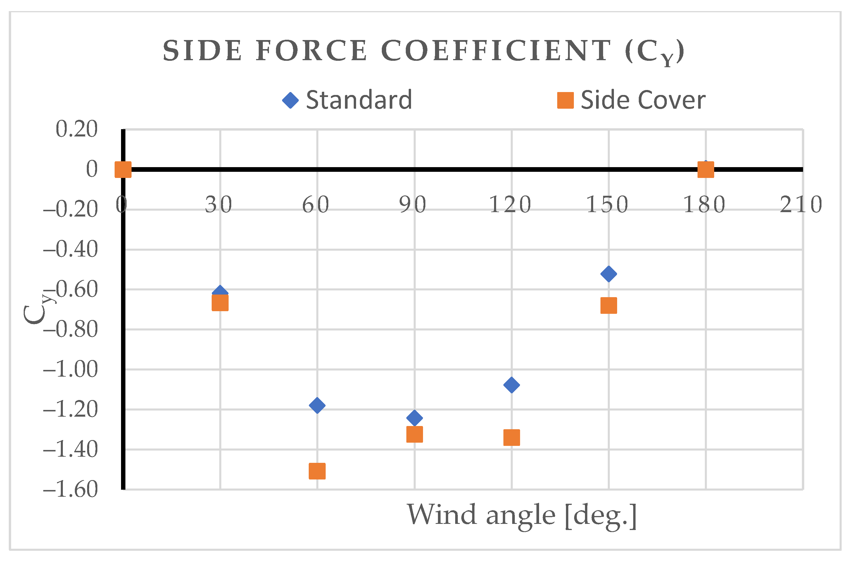
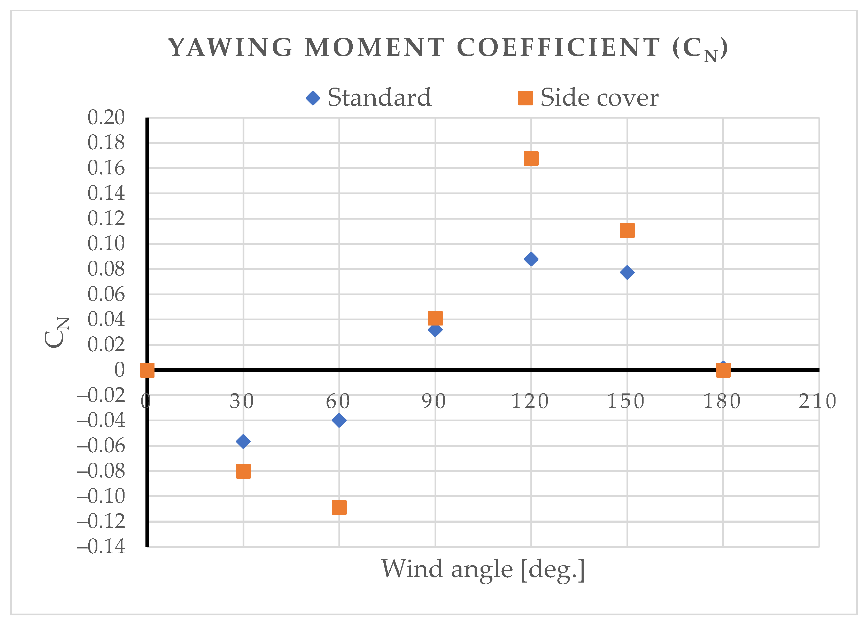
The effect of the side covers on wind forces and yaw moment coefficients at wind angles from 0 to 180 degrees are shown in Figure 34, Figure 35 and Figure 36. The calculated air resistance and the reduction ratio of the air resistance coefficient at 30 degrees are presented in Table 3. As shown in Table 3, the side covers reduce the air resistance acting on the ship model by up to 53% from that acting on the standard model. This is due to the reduction in the resistance acting on each container block when the gaps are shut by the side covers. In other words, the gap air flow is the major factor that increases air resistance, and air resistance in oblique winds can be reduced by shutting the gap air flow between the container blocks on deck. The air resistances shown in Figure 33 show that the side covers significantly reduce the resistance at a wind angle of 30 degrees and generate thrust at a wind angle of 60 degrees. It should be noted that, in following winds, the side covers reduce the thrust forces due to the winds. These results are consistent with the experimental study reported by (Ouchi et al., 2014). The side forces, as shown in Figure 35, demonstrate that the side covers at oblique winds increase the side forces by closing the gaps among deck containers, particularly at 60 and 120 degrees. The yaw moments shown in Figure 36 also show that the side covers also increase the yaw moment generated by winds at oblique winds.
4. Conclusions
The wind forces acting on a large container ship model carrying many containers on deck are numerically investigated by using CFD. The following conclusions are drawn from the calculations.
(1) High pressure acts on the upper half of the front surface of the first block of deck containers and the bow end of the hull. These high pressures may increase the air resistance on the ship.
(2) Flow separation occurs at the top of the front container block, and a wide wake including a three-dimensional vortex covers the top of the containers.
(3) The three-dimensional vortex above the top of containers leads to many air flows passing the gaps between container blocks. These complex flows may affect the characteristics of the air resistance acting on the ship.
(4) Air flows passing the gaps between container blocks are generated in oblique winds. At a wind angle of 30 degrees, the gap air flows create a separation bubble near the entrance of each gap. The gap air flows do not run through the gap horizontally and slow down near the center of each gap.
(5) High pressures are generated at each edge of the deck container blocks in the gaps leading to the increase in air resistance acting on the ship.
(6) By shutting the gap air flow, the air resistance acting on the ship can be reduced by 50% at a wind direction of 30 degrees and thrust can be produced at a wind direction of 60 degrees.
(7) Shutting the gap air flows leads to a consequential decrease in the thrust acting on the ship in oblique and following winds.
(8) Shutting the gap air flows also leads to an increase in the side force and the yaw moment due to the winds.
In terms of the aerodynamics of the ship, the side covers have advantages and disadvantages for ship performance, especially those characteristics affected by the air resistance factor. To design for and apply to real container ships, there are several factors one should consider before using side covers, such as the ship structures, loading conditions, maintenance problems, etc. In this study, we assumed that those factors do not influence container ship performance in headwinds and oblique winds.
Author Contributions
Conceptualization, V.T.N. and M.D.L.; methodology, V.M.N.; software, V.T.N.; validation, V.T.N., M.D.L. and V.M.N.; formal analysis, V.T.N.; investigation, V.T.N.; data curation, V.T.N.; writing—original draft preparation, V.T.N.; writing—review and editing, M.D.L. and V.M.N.; visualization, V.T.N.; supervision, T.K. and Y.I.; project administration, V.T.N.; funding acquisition, V.T.N. All authors have read and agreed to the published version of the manuscript.
Funding
This project is funded by The University of Danang and the Danang City Department of Science and Technology grant number B2019-DN01-23-HT.
Institutional Review Board Statement
Not applicable.
Informed Consent Statement
Not applicable.
Data Availability Statement
Not applicable.
Acknowledgments
The authors would like to express their special appreciation and thanks to The University of Danang and the Danang City Department of Science and Technology for the financial support to complete this project. The authors would also thank Osaka Metropolitan University for providing the research facilities and other support to this project.
Conflicts of Interest
The authors declare no conflict of interest.
References
- Koričan, M.; Perčić, M.; Vladimir, N.; Alujević, N.; Fan, A. Alternative Power Options for Improvement of the Environmental Friendliness of Fishing Trawlers. J. Mar. Sci. Eng. 2022, 10, 1882. [Google Scholar] [CrossRef]
- Pérez-Arribas, F.; Silva-Campillo, A.; Díaz-Ojeda, H.R. Design of Dihedral Bows: A New Type of Developable Added Bulbous Bows—Experimental Results. J. Mar. Sci. Eng. 2022, 10, 1691. [Google Scholar] [CrossRef]
- Riesner, M.; El Moctar, O.; Schellin, T. Design related speed loss and fuel consumption of ships in seaways. In Progress in Maritime Technology and Engineering; CRC Press: Boca Raton, FL, USA, 2018; pp. 147–155. [Google Scholar]
- Bialystocki, N.; Konovessis, D. On the estimation of ship’s fuel consumption and speed curve: A statistical approach. J. Ocean. Eng. Sci. 2016, 1, 157–166. [Google Scholar] [CrossRef] [Green Version]
- Zhou, T.; Hu, Q.; Hu, Z.; Zhen, R. An adaptive hyper parameter tuning model for ship fuel consumption prediction under complex maritime environments. J. Ocean Eng. Sci. 2022, 7, 255–263. [Google Scholar] [CrossRef]
- Luo, S.; Ma, N.; Hirakawa, Y. Evaluation of resistance increase and speed loss of a ship in wind and waves. J. Ocean Eng. Sci. 2016, 1, 212–218. [Google Scholar] [CrossRef] [Green Version]
- Vitali, N.; Prpić-Oršić, J.; Soares, C.G. Coupling voyage and weather data to estimate speed loss of container ships in realistic conditions. Ocean Eng. 2020, 210, 106758. [Google Scholar] [CrossRef]
- Haddara, M.R.; Soares, C.G. Wind loads on marine structures. Mar. Struct. 1999, 12, 199–209. [Google Scholar] [CrossRef]
- Fujiwara, T.; Tsukada, Y.; Kitamura, F.; Sawada, H.; Ohmatsu, S. Experimental Investigation and Estimation on Wind Forces for a Container Ship. Proc. Ninet. Int. Offshore Polar Eng. Conf. 2009, 1, 555–562. [Google Scholar]
- Szelangiewicz, T.; Wiśniewski, B.; Želazny, K. The Influence of Wind, Wave and Loading Condition on Total Resistance and Speed of the Vessel. Pol. Marit. Res. 2014, 21, 61–67. [Google Scholar] [CrossRef] [Green Version]
- Sugata, K.; Iwamoto, Y.; Ikeda, Y.; Nihei, Y. Reduction of Wind Force acting on Ships. Proc. APHydro2010 2010, 9480, 5–8. [Google Scholar]
- Andersen, P.; Borrod, A.-S.; Blanchot, H. Evaluation of the Service Performance of Ships. Mar. Technol. SNAME News 2005, 42, 177–183. [Google Scholar] [CrossRef]
- Karabulut, U.C.; Özdemir, Y.H.; Barlas, B. Numerical Investigation of the Effect of Surface Roughness on the Viscous Resistance Components of Surface Ships. J. Marine. Sci. Appl. 2022, 21, 71–82. [Google Scholar] [CrossRef]
- Andersen, I.M.V. Wind loads on post-panamax container ship. Ocean Eng. 2013, 58, 115–134. [Google Scholar] [CrossRef]
- Ouchi, K.; Tanaka, Y.; Taniguchi, A.; Takashina, J.; Matsubara, N.; Kimura, K. A study on air drag reduction on the large container ship in the sea. In Proceedings of the International Conference Design & Operation of Container Ships, London, UK, 21–22 May 2014; pp. 107–114. [Google Scholar]
- Kim, Y.; Kim, K.; Jeong, S.; Jeong, S.; Van, S.; Kim, Y.-C.; Kim, J. Design and Performance Evaluation of Superstructure Modification for Air Drag Reduction of a Container Ship. In Proceedings of the 25th International Ocean and Polar Engineering Conference (ISOPE), Big Island, HI, USA, 21 June–26 June 2020; pp. 894–901. [Google Scholar]
- Van He, N.; Mizutani, K.; Ikeda, Y. Reducing air resistance acting on a ship by using interaction effects between the hull and accommodation. Ocean Eng. 2016, 111, 414–423. [Google Scholar] [CrossRef]
- Van He, N.; Hien, N.; Truong, V.-T.; Bui, N.-T. Interaction Effect between Hull and Accommodation on Wind Drag Acting on a Container Ship. J. Mar. Sci. Eng. 2020, 8, 930. [Google Scholar] [CrossRef]
- Watanabe, I.; Nguyen, V.T.; Miyake, S.; Shimizu, N.; Ikeda, Y. A Study on Reduction of Air Resistance acting on a Large Container Ship. In Proceedings of the APHydro2016, Hanoi, Vietnam, 20–23 September 2016; pp. 321–330. [Google Scholar]
- Nguyen, V.T.; Kinugawa, A.; Shimizu, N.; Ikeda, Y. Studies on Air Resistance Reduction Methods for a Large Container Ship (Part 1). In Proceedings of the JASNAOE Annual Autumn Meeting, Okayama City, Japan, 21–22 November 2016; pp. 427–432. [Google Scholar]
- Blocken, B.; Stathopoulos, T.; van Beeck, J. Pedestrian-level wind conditions around buildings: Review of wind-tunnel and CFD techniques and their accuracy for wind comfort assessment. Build. Environ. 2016, 100, 50–81. [Google Scholar] [CrossRef]
- ITTC. Practical Guidelines for Ship CFD Application. In Proceedings of the 26th International Towing Tanks Conference, Rio de Janeiro, Brazil, 28 August–3 September 2011; Number 7.5-03-02-03; ITTC: 2011. Available online: https://ittc.info/media/1357/75-03-02-03.pdf (accessed on 20 December 2022).
- Van Nguyen, T.; Kinugawa, A. Development of Practical Gap Covers to Reduce Air Resistance Acting on Deck Containers of a Ship. In Proceedings of the 23th conference Japan Society of Naval Architects and Ocean Engineers, Hiroshima, Japan, 27–28 November 2017; pp. 211–216. [Google Scholar]
- Van Nguyen, T. Vortex Control in Gap Flow by Small Appendages to Reduce Air Resistance Acting on Deck Containers of a Ship. In Proceedings of the 24th Conference Japan Society of Naval Architects and Ocean Engineers, Tokyo, Japan, 26 May 2017; pp. 335–338. [Google Scholar]
- Pena, B.; Huang, L. A review on the turbulence modelling strategy for ship hydrodynamic simulations. Ocean Eng. 2021, 241, 110082. [Google Scholar] [CrossRef]
Figure 1.
Side and frontal profiles of the modeled container ship in a fully loaded condition.

Figure 2.
Computational domains.

Figure 3.
Coordinate system with wind direction.

Figure 4.
Global mesh. (a) Cut mesh at the symmetry plane, (b) Cut mesh at the horizontal plane.

Figure 5.
Local mesh near the gap.

Figure 6.
Comparison of the longitudinal force coefficients (Cx) between CFD and Experiment.

Figure 7.
Locations of velocity profiles 1-1 to 3-3 (z = 0.12 m, =30 deg.).

Figure 8.
Velocity profile at the upstream section (1-1).

Figure 9.
Velocity profile at the center section (2-2).

Figure 10.
Velocity profile at the downstream section (3-3).

Figure 11.
Streamlines around the container ship.

Figure 12.
Velocity vectors near the gap entrance ( = 30 deg.).

Figure 13.
Velocity profile at cross-section (4-4) in the gap between containers.

Figure 14.
Velocity profile at cross-section (10-10) in the gap between containers.

Figure 15.
Pressure distribution in and around the gap between I-I and II-II.

Figure 16.
The coefficients of the pressure difference between (I-I) and (II-II).

Figure 17.
Pressure distributions around the engine casing.

Figure 18.
Coefficient of the pressure difference between E1–E2.

Figure 19.
Coefficient of the pressure difference between E4-E3.

Figure 20.
Velocity vectors of gap air flow near engine casing.

Figure 21.
Streamlines of gap air flow near engine casing.

Figure 22.
Pressure near the accommodation house.

Figure 23.
Difference of pressure between A1-A2.

Figure 24.
Difference of pressure between A4-A3.

Figure 25.
Velocity vectors in the gap in which an accommodation house is located.

Figure 26.
Streamlines in the gap at an accommodation house.

Figure 27.
Ship model with side covers.

Figure 28.
Pressure distributions around the container ship with (Right) and without (Left) side covers in oblique winds at z = 0.12 m, = 30 deg.
Figure 28.
Pressure distributions around the container ship with (Right) and without (Left) side covers in oblique winds at z = 0.12 m, = 30 deg.

Figure 29.
(a). Pressure acting on the frontal surface, z = 0.12 m, = 30 degrees. (Left: without side covers; Right: with side covers). (b). Comparison of pressure acting on the frontal surface, z = 0.12 m, = 30 degrees. (FP: Front-Port side, FS: Front-Starboard).
Figure 29.
(a). Pressure acting on the frontal surface, z = 0.12 m, = 30 degrees. (Left: without side covers; Right: with side covers). (b). Comparison of pressure acting on the frontal surface, z = 0.12 m, = 30 degrees. (FP: Front-Port side, FS: Front-Starboard).


Figure 30.
(a). Pressure acting on the back surface, z = 0.12 m, = 30 degrees. (Left: without side covers; Right: with side covers; BP: Back-Port side, BS: Back-Starboard). (b). Comparison of pressure acting on the back surface, z = 0.12 m, =30 degrees.
Figure 30.
(a). Pressure acting on the back surface, z = 0.12 m, = 30 degrees. (Left: without side covers; Right: with side covers; BP: Back-Port side, BS: Back-Starboard). (b). Comparison of pressure acting on the back surface, z = 0.12 m, =30 degrees.


Figure 31.
Velocity at z = 0.12 m, = 30 degrees. (Left: without side covers; Right: with side covers).
Figure 31.
Velocity at z = 0.12 m, = 30 degrees. (Left: without side covers; Right: with side covers).

Figure 32.
Streamline from z = 0.12 m, = 30 degrees. (Left: without side covers; Right: with side covers).
Figure 32.
Streamline from z = 0.12 m, = 30 degrees. (Left: without side covers; Right: with side covers).

Figure 33.
Velocity vector near the bow, at z = 0.12 m, = 30 degrees. (Left: without side covers; Right: with side covers).
Figure 33.
Velocity vector near the bow, at z = 0.12 m, = 30 degrees. (Left: without side covers; Right: with side covers).

Figure 34.
Effect of side covers on the resistance coefficient at different wind angles.

Figure 35.
Effect of side covers on the side force coefficient at different wind angles.

Figure 36.
Effect of side covers on the yawing moment coefficient at different wind angles.


Table 1.
Principal particulars of ship and model.
| Specifications | Unit | Ship | Model |
|---|---|---|---|
| — | 1/255.3 | ||
| Length of Overall (LOA) | [m] | 400 | 1.560 |
| Length Between Perpendicular (LPP) | [m] | 383 | 1.50 |
| Breadth (B) | [m] | 58.5 | 0.230 |
| Depth (H) | [m] | 32.06 | 0.1250 |
| Draft (d) | [m] | 14.5 | 0.0570 |
| Frontal Projected Area (AF) | [m2] | 2890 | 0.0443 |
| Side Projected Area (AS) | [m2] | 18,000 | 0.2762 |
Table 2.
Solution setup.
| Solver | |
|---|---|
| Type | Pressure-Based |
| Velocity formulation | Absolute |
| Time | Steady |
| Models | |
| Viscous model | k-epsilon (2 eqs) |
| k-epsilon Model | Standard |
| Near-Wall Treatment | Standard Wall Functions |
| Materials | |
| Fluid | Air |
| Properties | |
| Density | 1.225 (kg/m3) |
| Viscosity | 1.7894 × 10⁻⁵ |
| Boundary Conditions | |
| Inlet | Velocity inlet: Velocity Magnitude: 10 (m/s) Turbulent Intensity: 5% Turbulent Viscosity Ratio: 10 |
| Outlet | Pressure outlet: Backflow Turbulent Intensity: 5% Backflow Turbulent Viscosity Ratio: 10 |
| Ship | Wall: No Slip |
| Top, bottom, sidewalls | Wall: Slip |
| Solution Methods | |
| Pressure-Velocity Coupling | |
| Scheme | SIMPLE |
| Spatial Discretization | |
| Gradient | Least Squares Cell-Based |
| Pressure | Standard |
| Momentum | Second-Order Upwind |
| Turbulent Kinetic Energy | Second-Order Upwind |
| Turbulent Dissipation Rate | Second-Order Upwind |
Table 3.
Resistance coefficient and reduction of resistance coefficient at a wind direction of 30 degrees.
Table 3.
Resistance coefficient and reduction of resistance coefficient at a wind direction of 30 degrees.
| Model | Cx | ΔCx (%) (*) |
|---|---|---|
| Standard | −0.90118 | |
| Side cover | −0.42042 | −53.35 |
(*) Reduction of resistance coefficient: .
Disclaimer/Publisher’s Note: The statements, opinions and data contained in all publications are solely those of the individual author(s) and contributor(s) and not of MDPI and/or the editor(s). MDPI and/or the editor(s) disclaim responsibility for any injury to people or property resulting from any ideas, methods, instructions or products referred to in the content. |
© 2023 by the authors. Licensee MDPI, Basel, Switzerland. This article is an open access article distributed under the terms and conditions of the Creative Commons Attribution (CC BY) license (https://creativecommons.org/licenses/by/4.0/).
Share and Cite
MDPI and ACS Style
Nguyen, V.T.; Le, M.D.; Nguyen, V.M.; Katayama, T.; Ikeda, Y. Influences of Gap Flow on Air Resistance Acting on a Large Container Ship. J. Mar. Sci. Eng. 2023, 11, 160. https://doi.org/10.3390/jmse11010160
AMA Style
Nguyen VT, Le MD, Nguyen VM, Katayama T, Ikeda Y. Influences of Gap Flow on Air Resistance Acting on a Large Container Ship. Journal of Marine Science and Engineering. 2023; 11(1):160. https://doi.org/10.3390/jmse11010160
Chicago/Turabian StyleNguyen, Van Trieu, Minh Duc Le, Van Minh Nguyen, Toru Katayama, and Yoshiho Ikeda. 2023. "Influences of Gap Flow on Air Resistance Acting on a Large Container Ship" Journal of Marine Science and Engineering 11, no. 1: 160. https://doi.org/10.3390/jmse11010160
Note that from the first issue of 2016, this journal uses article numbers instead of page numbers. See further details here.