
Importance of Pre-Storm Morphological Factors in Determination of Coastal Highway Vulnerability


1
Department of Civil and Environmental Engineering, University of Illinois Urbana-Champaign, 2521 Hydrosystems Lab, 205 N. Mathews Ave., Urbana, IL 61801, USA
2
Civil, Construction, and Environmental Engineering Dept., North Carolina State University, Raleigh, NC 27695, USA
*
Author to whom correspondence should be addressed.
J. Mar. Sci. Eng. 2022, 10(8), 1158; https://doi.org/10.3390/jmse10081158
Submission received: 15 June 2022
/
Revised: 30 July 2022
/
Accepted: 17 August 2022
/
Published: 21 August 2022
(This article belongs to the Special Issue Performance of Transportation Systems Subjected to Extreme Hydrodynamic Events)
Abstract
:This work considers a database of pre-storm morphological factors and documented impacts along a coastal roadway. Impacts from seven storms, including sand overwash and pavement damage, were documented via aerial photography. Pre-storm topography was examined to parameterize the pre-storm morphological factors likely to control whether stormwater levels and waves impact the road. Two machine learning techniques, K-nearest neighbors (KNN) and ensemble of decision trees (EDT), were employed to identify the most critical pre-storm morphological factors in determining the road vulnerability, expressed as a binary variable to impact storms. Pre-processing analysis was conducted with a correlation analysis of the predictors’ data set and feature selection subroutine for the KNN classifier. The EDTs were built directly from the data set, and feature importance estimates were reported for all storm events. Both classifiers report the distances from roadway edge-of-pavement to the dune toe and ocean as the most important predictors of most storms. For storms approaching from the bayside, the width of the barrier island was the second most important factor. Other factors of importance included elevation of the dune toe, distance from the edge of pavement to the ocean shoreline, shoreline orientation (relative to predominant wave angle), and beach slope. Compared to previously reported optimization techniques, both machine learning methods improved using pre-storm morphological data to classify highway vulnerability based on storm impacts.
1. Introduction
Coastal road infrastructure represents one of the main components of cities located at or near the ocean. This infrastructure suffers inevitable damage due to natural hazards that pose not only life-threatening events to population, but also a burden to the satisfactory operation of infrastructure [1]. In the United States, there is an average general cost of 20.5 billion USD per hurricane each year at places exclusively located close to shorelines [2]. Particularly, the state of North Carolina, which has the second largest shoreline (484 km) of the US Atlantic coast, reported a value of 181 million USD, on average, over the years of 2016 and 2020, due to the presence of inclement weather events, such as hurricanes [3]. In recent years, local authorities have conducted prevention programs, including the regular measurement of the physical characteristics of coastal areas. These data-collecting efforts have guided researchers and transportation agencies to perform prevention-related activities, such as the development of vulnerability indicators for coastal roadways. The analysis of these indicators may provide a better understanding of the drivers of coastal roadway vulnerability and assist transportation departments with preventive actions in response to natural hazards.
Pre-storm coastal morphology, in partnership with storm properties (waves and storm surge), has long been assumed to control impacts on beaches, dunes, barrier islands, and the infrastructure present on those islands. Coastal morphology features, including island width, dune crest elevation, and distance from the road edge to the ocean shoreline, are indicators to assess whether road infrastructure is vulnerable to damage or not [4]. Vulnerability analysis reflects the susceptibility of the infrastructure to reduce its functionality, ranging from debris removal without interruption to temporary road closures [5]. Processes such as storm surges and sea-level rise are the main drivers of the overall damage to coastal infrastructure. Previous research works and agency reports agree that the increment in the number of storms and rising sea levels will likely affect coastal communities at different severity levels [6,7]. Furthermore, as mentioned by [8], there is a need for local coastal road systems to handle dynamic conditions. This work aims to contribute to the literature by developing a classifier model coupling past storm information with current and historical local morphology factors to inform stakeholders of the vulnerability of coastal roadways to hurricanes and tropical storms.
The monitoring of areas close to coastal roadways provides critical information about the past and current conditions of the existing road infrastructure. Especially in barrier islands, where bridges and roadways are likely the first infrastructure systems facing the ocean, monitoring indicators have provided managers valuable insights for beach restoration projects and natural habitat conservation programs [9,10]. Moreover, state agencies use field-measured data coupled with visualization from aerial photographs to monitor the morphological conditions of coastal zones, such as barrier islands, over time, especially after natural hazards events. Therefore, modeling and analyzing these dynamic data sets are the backbone of the current and future action plans to protect coastal infrastructure, such as roadways.
Recently, machine learning techniques have been explored to inform land cover classifications and storm responses [10]. A review of machine learning techniques to classify land cover is provided by [11], with the random forest algorithm having the highest accuracy level for this application. An examination of machine learning in land use and cover change detection and modeling was provided by [12]. These authors stated that machine learning has the strong potential to advance the modeling of land use and cover changes by identifying and incorporating new exploratory variables.
An application of machine learning to storm response and recovery, considering power utility, was detailed by [13]. The authors developed a data-driven predictive model to aid the utility in its emergency planning efforts. Another power utility application was presented in [14], with a focus on quantification of uncertainty in machine-learning-based prediction modeling. Other works have focused on predicting physical and social storm impacts; ref. [15] developed a convolutional-neural-network-based model to rapidly predict storm surge across an extensive coastal region using a storm track. Other studies have examined storm impacts and responses via social media data [16,17,18].
In parallel to the machine learning work, much work regarding the control of variable storm impacts has focused on damage to protective dunes [19,20]. These studies linked controls on hydrodynamic forcing to erosion of the dune. Recently, ref. [5] developed a data set of seven storms and the corresponding impacts on a coastal highway, along with a robust collection of varying morphological factors that could be used to predict impact. They used deterministic optimization techniques (i.e., mixed integer linear programming) and found that the distance from edge-of-pavement to dune toe, volume above mean high water between edge-of-pavement and ocean shoreline, distance from edge-of-pavement to ocean shoreline, and dune crest height above the road were the most skilled individual predictors of highway vulnerability. A multi-indicator function of dune toe elevation and distance from edge-of-pavement to dune toe was found to be more skilled than any of the individual indicators.
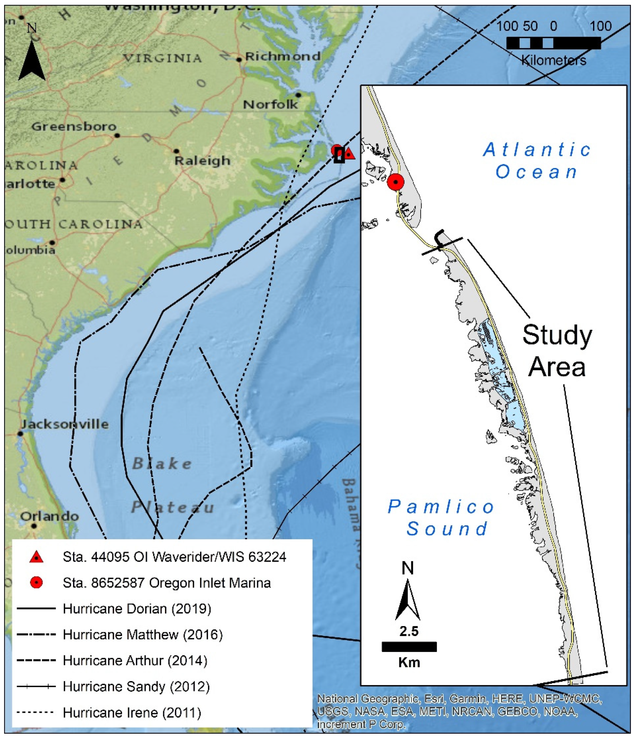
This paper aims to apply two machine learning techniques to the storm impact data set presented in previous studies [5], in order to classify roadway vulnerability and identify the indicators that best infer storm impacts. We applied two classifiers, K-nearest neighbor (KNN) and ensemble of decision trees (EDT), to classify whether different longitudinal segments or transects of a coastal roadway are considered vulnerable (class of interest) or not. Our models were applied to a 13-mile (21-km) expanse of state highway North Carolina 12 (NC 12), along Hatteras Island, NC (Figure 1). NC 12 is an essential, 148.0-mile-long (238.2 km) coastal highway that connects Corolla to Cedar Island on the northern side of the Outer Banks in the state of North Carolina, USA [4].
2. Materials and Methods
2.1. Dataset
This section describes the data set and methods used in the analysis. The data sets comprise seven groups, corresponding to seven storm events registered by the North Carolina Department of Transportation (NCDOT) between 2011 and 2019 [4]. The storms featured in this paper are summarized in Table 1. Of the seven storms in the data set, five were hurricanes, and their tracks, in relation to the study area, are shown in Figure 1. Two of the storms in the data set were winter extra-tropical storms, or “nor’easters”, which are not tracked in the same way as hurricanes. Locations of storm impacts to the study area’s highway, NC 12, were identified for each of the seven storms. Aerial imagery from the National Oceanic and Atmospheric Administration (NOAA) national geodetic survey and imagery, collected under the NCDOT Coastal Monitoring Program [4], were manually examined at the 1:1250 scale to locate road impacts along NC 12 (Table 1). These data collection efforts were described in detail in [5] and summarized in this section. A section of roadway was determined to be impacted if more than 50 percent of the roadway was covered with sand or visibly damaged. In general, post-storm imagery was available on the order of days post-storm, which precluded the inclusion of visible flooding as a storm impact, as it had already receded.
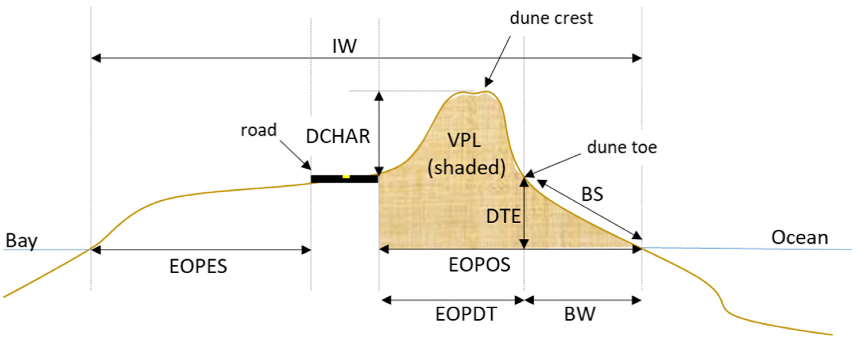
The indicators used to determine an impacted road transect are numerical values of the geomorphologic characteristics extracted from the coastal features of the area; they are listed in Table 2 and illustrated in the schematic in Figure 2 [5]. Most of the geomorphological measurements provided in Table 2 are straightforward and visible in Figure 2. It is noted that the shoreline was identified as the visible wet-dry line on aerial photographs and is approximately the mean high-water line [21]. In this area, the mean high-water elevation is approximately 1.1 ft (0.34 m) above the North American Vertical Datum of 1988 (NAVD88) [22]. The “angular difference between shore-normal orientation and weighted mean wave direction”, however, is a bit complicated to illustrate. The hypothesis was that the shore’s orientation can be used as a proxy for exposure to average storm waves. Transects along the study area that are more exposed to direct storm waves are more likely to see significant erosion and overwash, which can affect the highway. To calculate the weighted mean wave direction (similar to the weighted mean wind direction used by [23]), wave data from the Oregon Inlet waverider buoy (NDBC station 8652587, Figure 1), between 2012–2020, were filtered to only include significant wave heights greater than 2 m, and wave direction was weighted by the square of significant wave height to better represent the directional distribution of wave energy. Circle statistics functions were used to ensure that angular directions were preserved. The mean wave direction was assumed to be constant across the relatively small (13-mile, 21-km) study area. The orientation of a line normal to the shore at each transect was computed at each transect along the study area. The angular difference between the wave height weighted mean wave direction and shore-normal orientation was computed on a transect basis. The measurement could vary from 0 to 90 degrees, where 0 degrees would suggest that the shoreline is most exposed to the average storm wave direction, and 90 degrees would be most sheltered from the mean storm wave impact.
The binary outputs of each data set assign 0 if the road transect was not impacted by a storm and 1 otherwise. These data sets have an imbalance problem, as the class of interest (impacted road transect or 1) happens less frequently than the not impacted road class (0). Therefore, the evaluation of the proposed methodology includes metrics of performance that reduce this implicit bias from the results, as explained below.
2.2. Correlation Analysis
A correlation analysis was performed to identify linear dependence among predictors prior to building one classification model, as explained below. The correlation matrix, where rows represent observations and columns the variables, shows the Pearson correlation coefficient calculated as shown in Equation (1):
where A and B are two random variables with N observations; µ and σ are the mean and standard deviations of A and B, respectively.
The preprocessing step filters predictors based on the correlation () and implements a feature selection subroutine. The Chi-square test reports low p-values when the corresponding predictor is dependent on the response variable and considered an important feature. If between two variables is equal to or higher than 0.95 (e.g., considered perfectly correlated), the most important feature reported by the Chi-square test remains in the data set.
2.3. Binary Classifiers
We apply two widely known classifiers methods for binary classification as the K-nearest neighbors (KNN) [25] and the ensemble of decision trees (EDT) [26]. These two classifiers were selected because KNN and EDT have been proven as classifiers that effectively handle imbalanced data sets [27,28,29]. For the KNN classifier, we filter perfectly correlated variables based on their rank correlation and select the most important predictors based on a feature selection subroutine that uses the Chi-square test [30]. This step avoids inflating the distance from correlated predictors. Decision trees do not assume relationships between features, but split data into subsamples that boost their classification performance. To overcome overfitting issues, related to creating a single decision tree, we use the EDT model that improves its performance, albeit decreasing interpretability. Additionally, these classifiers are not considered black boxes with random initial parameters, which makes them feasible to reproduce for similar potential problems.
2.3.1. K-Nearest Neighbor (KNN)
KNN is a simple supervised-learning classifier that assigns a new variable to the class with the most values from the closest k neighbors located on a search space, determined by the number of predictors [25]. The two inputs required to train and predict a KNN model are the number of neighbors (k) and type of distance used to determine the closest neighbors in a jth dimension, where j corresponds to the number of predictors (Figure 3). In this work, we performed an optimization subroutine to find the best hyperparameters of the KNN model for each storm. A Bayesian optimization algorithm [31] was applied to improve the performance of the KNN classifier model for each storm. The Bayesian optimization subroutine decision variables include the number of neighbors, distance metric, distance weight, and whether the data are standardized. Table 3 shows the search range used for the hyperparameter optimization of the KNN model [32].
KNN takes, as response, a binary variable called impact, where 1 represents the road is vulnerable to storms impacts and 0, otherwise. The model includes the most important features retrieved from the correlation analysis and feature selection subroutine as predictors. These features, as shown in Table 2, include (1) island width (ft), (2) dune crest elevation (ft), (3) road elevation (ft), (4) dune crest height above road (ft), (5) EOP to ocean shore (ft), (6) volume per length (ft3/ft), (7) EOP to estuary shore (ft), (8) beach width (ft), (9) beach slope, (10) dune toe elevation (ft), (11) EOP to dune toe (ft), and (12) shore orientation (degrees).
2.3.2. Ensemble of Decision Trees (EDT)
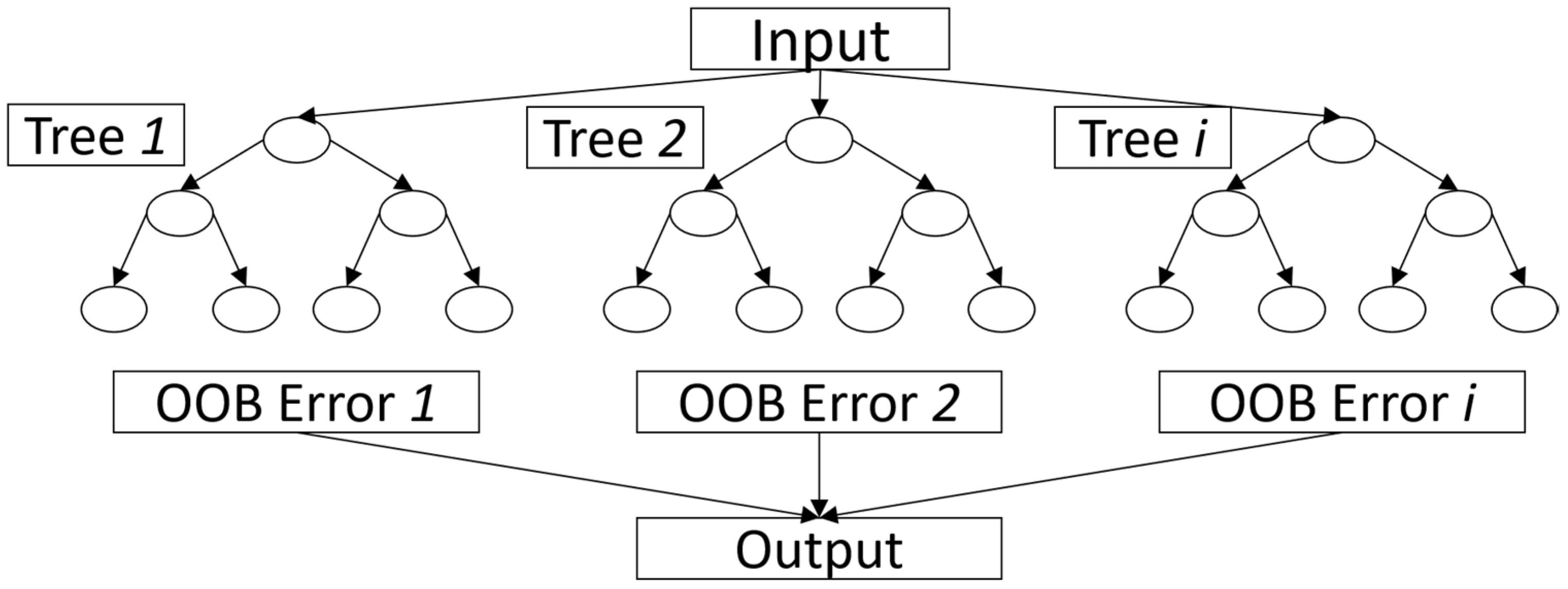
Decision trees are part of machine learning methods widely applied in the water quality, risk assessment, and forecasting domains to classify the risk of events, including pipe failure and water quality problems [27,28,29,33]. Decision trees graphically represent a classification or regression problem. The components of a single decision tree include a root node, internal nodes, and terminal nodes (see Figure 4). For classification models, a decision tree starts by assigning a class label to each leaf node. The non-terminal nodes, which include the root and other internal nodes, contain feature test conditions to separate records that have distinct characteristics. The root node has no incoming edges and can have multiple outgoing edges. Each internal node has exactly one incoming edge and two or more outgoing edges, and each leaf node has exactly one incoming edge and no outgoing edges [27,28,33,34]. In terms of bias and variability, a decision tree has low bias and high variance; therefore, averaging the result of many decision trees reduces the variance, while maintaining low bias. The application of ensembles enhances the performance of a single tree. Ensemble of decision trees (EDTs) group individual trees as one model to predict or fit numerical and categorical data (Figure 4). EDTs are built by comparing the “out-of-bag” (OOB) error value from all the individual decision trees and a voting combination of their results. EDTs have proved to be more robust when dealing with bias and variance, thus leading to generally a better prediction performance. However, EDTs are complex models to analyze, compared to individual decision trees [35].
EDTs start by identifying the root node. We used the well-known Gini index (Gidx) (Equation (2)) of a node as the split criterion to identify the root node of each tree in the ensemble. The Gidx with the lowest value is selected as the root node, and each tree grows until no more features remain for splitting [36]. EDTs are built using mainly two types of methods: bootstrap aggregation (bagging) and boosting. Bagging creates data set replicas using bootstrapping to incorporate single decision trees. A random selection of the observations with replacement is applied to create the bootstrap replicas. The most common application of bagging is the random forest method [36], where every tree of the ensemble randomly selects predictor variables for each split along the decision tree. Boosting methods, on the other hand, build the ensemble sequentially by using the output of the previous decision tree as input for the next one. The adaptive logistic regression (LogiBoost) algorithm, which is a variation of the adaptive boosting methods, can improve model performance when dealing with binary classification problems [37]. LogiBoost is a type of the widely applied adaptive boosting algorithm, where the objective function is to minimize the binomial deviance rather than the exponential loss, as shown in Equation (3):
where pr is the probability of an observation i classified into a particular class.
where:
- is the true class label;
- are normalized weights;
- is the predicted classification score calculated, as shown in Equation (4):
- are weights of the weak hypotheses () in the ensemble that are used to determine weighted error (), as shown in Equation (5):
- is a vector of predictor values for observation n;
- is the true class label;
- is the prediction of learner with index t;
- is the indicator function;
- is the weight of observation n at time step t.
In this study, we implemented a binary classification based on the analysis of the impacted roads with data collected from a set of storms that struck the North Carolina coast between 2011 and 2018.
2.3.3. EDT Settings
The number of trees or learners, their depth, and the overall learning rate are needed to set up an EDT model. Accuracy improves with the number of trees but also increases EDT’s complexity and computation time. Based on previous applications in water-related problems [27,28,29,33] and a series of preliminary analyses to determine the number of trees, a range between 10 and 100 trees was evaluated. A suitable option was found at 27 trees for the ensemble, as the performance did not improve with more trees. The maximum number of splits determines how deep a tree can be expanded. We analyzed a range between 10 and 100 observations, where 34 splits per tree produced the best results. Similarly, the learning rate that defined the step size of the error minimization was analyzed between 0.01 and 1.0, and a value of 0.65 was defined as suitable for the application of this model.
2.3.4. Model Training and Testing
The data sets for each storm were randomly partitioned into training (70%), validation (10%), and testing (20%) sets. Based on previous applications [33], each model was trained ten times to account for the stochasticity of the sampling method, and the average metrics of performance associated with each storm are reported as the results of the analysis. For the application of each classifier method, we optimize its hyperparameters, using the validation subset of each storm. Additionally, we compare the performance of these two classifiers using metrics that include the F1 score and precision-recall area under the curve (PR AUC) values, which are suitable for dealing with imbalanced data sets [38]. Finally, feature selection is presented to give a comprehensive analysis of the predictors with different effects on the model performance.
2.4. Metrics of Performance
The performance of classification models uses a set of commonly known metrics that are calculated using the confusion matrix, which shows the performance of a model in predicting samples within four classes (Table 4). True positives (TP) and true negatives (TN) denote the number of positive and negative events that are correctly identified, respectively. In this research, positive events correspond to events with a value of 1, which means that the predicted and observed outputs are vulnerable, and negative events correspond to events with a value of 0, which means that predicted and observed outputs are not vulnerable. False positives (FP) denote the number of not vulnerable events incorrectly identified as vulnerable, and false negatives (FN) indicate the number of vulnerable events incorrectly identified as not vulnerable. Performance metrics, including accuracy (Equation (6)), precision (Equation (7)), recall (Equation (8)), and the F-1 score (Equation (9)), were calculated using the confusion matrix, as follows.
3. Results
3.1. Correlation Analysis and Feature Selection
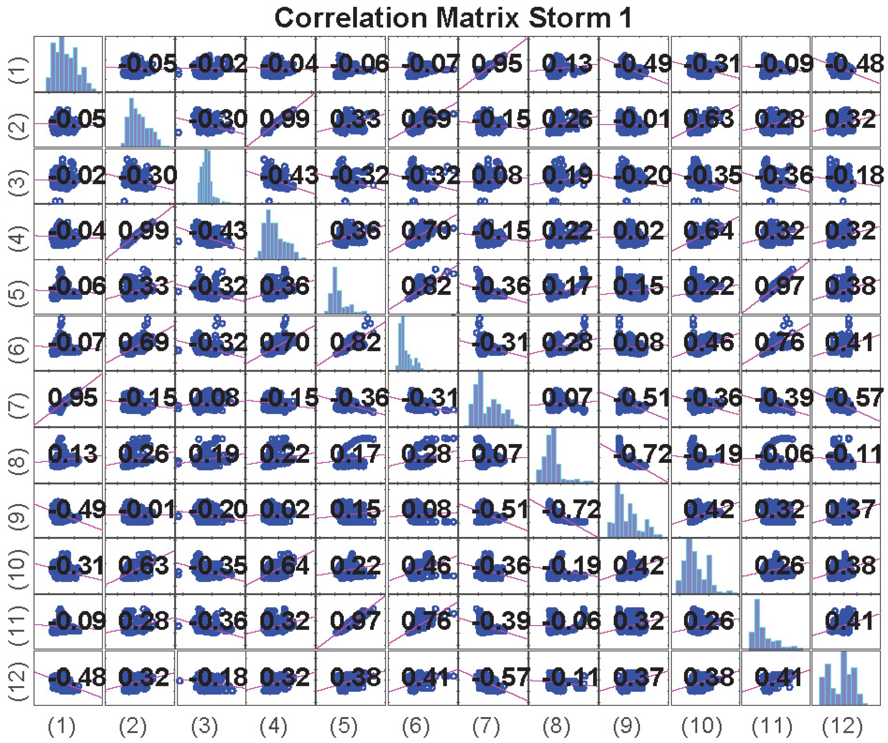
This section reports on the correlation analysis and feature selection subroutine applied prior to the KNN implementation. Then, the performance metrics of the two machine learning methods used for the binary classification problem are discussed. The correlation analysis (Equation (1)) of the predictors shows that, for all storm events, Pearson’s correlation coefficient indicates perfect correlation among several variables. As expected, “(1) Island Width” is perfectly correlated to “(7) EOP to Estuary Shore”; “(2) Dune Crest Elevation” correlated to “(4) Dune Crest Height above Road”; and “(5) EOP correlated to Ocean Shore” to “(11) EOP to Dune Toe” (Figure 5).
Feature selection is used to determine which perfectly correlated variable remains in the predictors’ data set. Using the Chi-square test, the method reports that “Island Width” is a slightly better estimate than “EOP to Estuary Shore“ for storm events 1 to 5 (Figure 6a–e), and the opposite occurs for storms 6 and 7 (Figure 6f–g). Similarly, “Dune Crest Height above Road” is more important than “Dune Crest Elevation” for all storms, except for storm 5. Finally, “EOP to dune toe” is a better predictor than “EOP to Ocean” for all storms, except for storm 4 (Figure 6).
3.2. KNN and EDT Performances
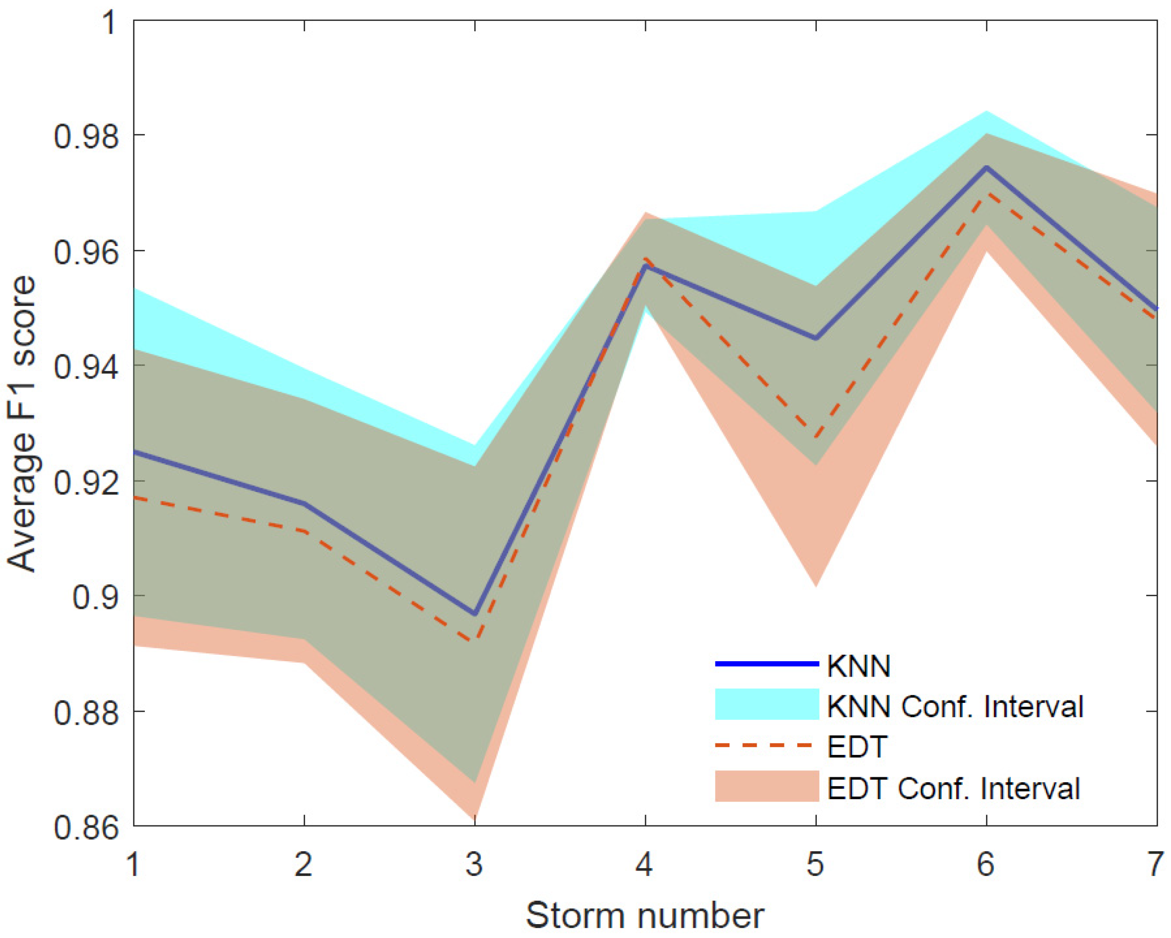
The classifier performances (Figure 7) show that the F-1 score reported by the KNN classifier looks similar to the EDT classifier’s F-1 score across the seven storm events. However, the KNN F-1 score had a slightly higher value than EDT in all storms, except storm number 4. We performed a t-test to examine the statistical relevance of the difference between the reported F-1 scores. The following hypothesis was evaluated:
- H0 = The pairwise difference between F-1 scores from KNN and EDT has a mean equal to zero at the 5% significance level.
- HA = The pairwise difference between F-1 scores from KNN and EDT has a mean not equal to zero at the 5% significance level.
The two-tailed t-rest resulted in a p-value of 0.04, indicating that the test rejects the null hypothesis (H0) of having identical mean values, in favor of the alternate hypothesis (HA) that the mean KNN F-1 score is significantly different than that of the EDT F-1 score at the 5% significance level.
The KNN and EDTs models’ performance, in terms of the F-1 score, shows that the models correctly classified a coastal road as vulnerable, based on the morphological indicators, at least 90% of the time. In the remaining 10%, the methods cannot classify an observation into the correct class. These high F-1 score values demonstrate the robustness of the classifiers to handle an imbalanced data set, where the class of interest (i.e., the road is vulnerable) is less frequent than the majority class (i.e., the road is not vulnerable to impact).
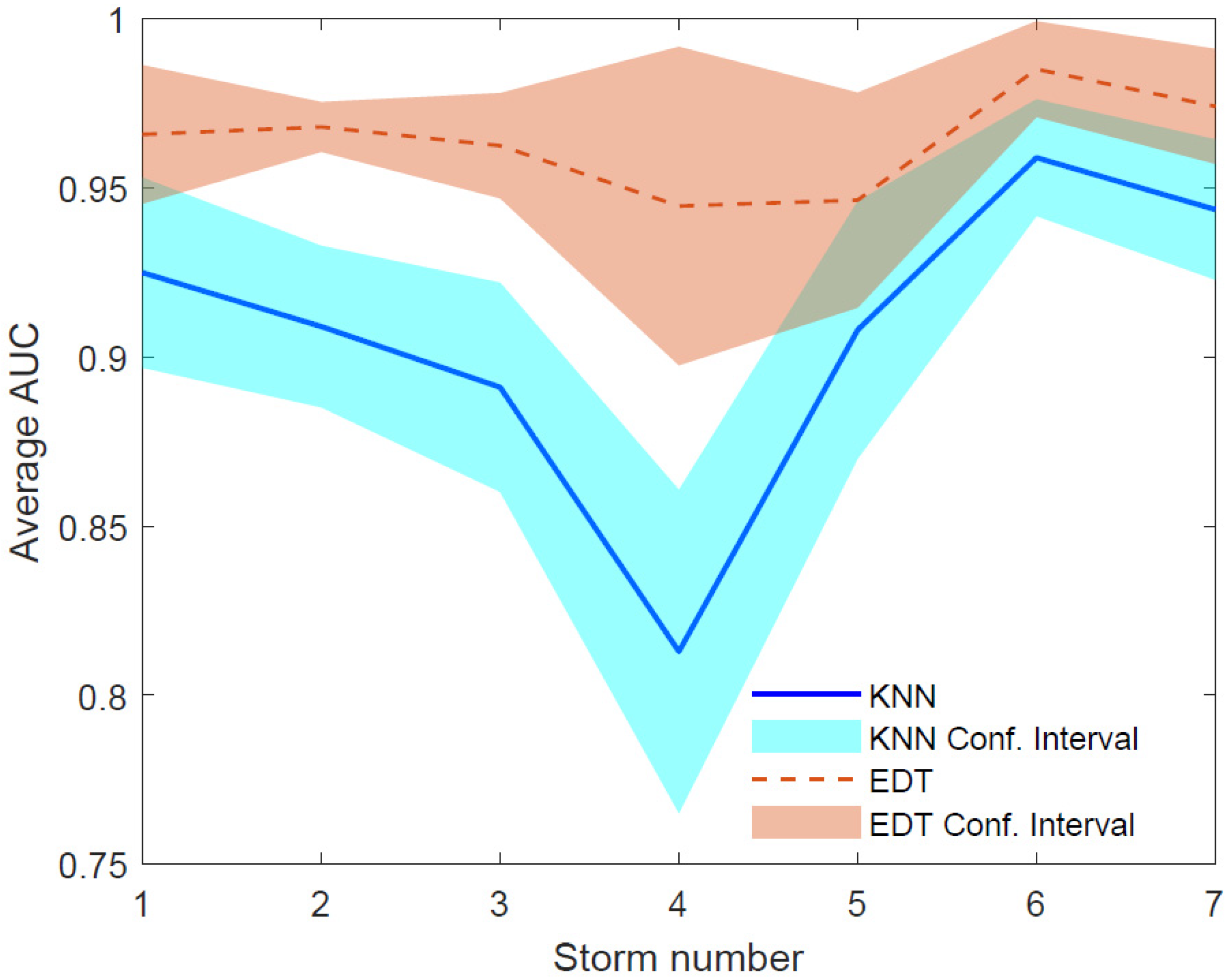
In terms of the area under the curve (AUC) reported by the classifiers, the EDT outperformed KNN classifier across the seven storms events (Figure 8). Both classifiers reported their maximum value during the storm event number 6, where KNN AUC represented 97% of EDT AUC. This difference increased for the lowest performance of both classifiers that occurs during storm event number 4, where KNN AUC only represented 86% of EDT AUC. Similar to the F-1 score analysis, the following hypothesis of the AUC values was evaluated:
- H0 = The pairwise difference between AUC values from KNN and EDT has a mean equal to zero at the 5% significance level.
- HA = The pairwise difference between AUC values from KNN and EDT has a mean not equal to zero at the 5% significance level.
The two-tailed t-test resulted in a p-value of 0.0063, indicating that the test rejects the null hypothesis (H0) of having identical mean values, in favor of the alternate hypothesis (HA) that the mean KNN AUC value is significantly different than that of the EDT AUC value at the 5% significance level.
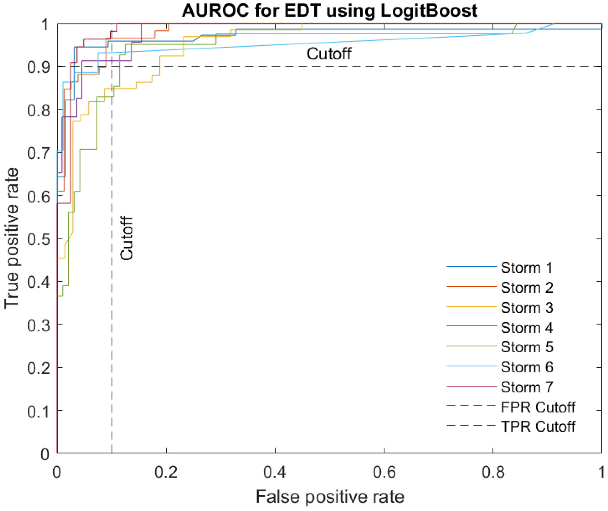
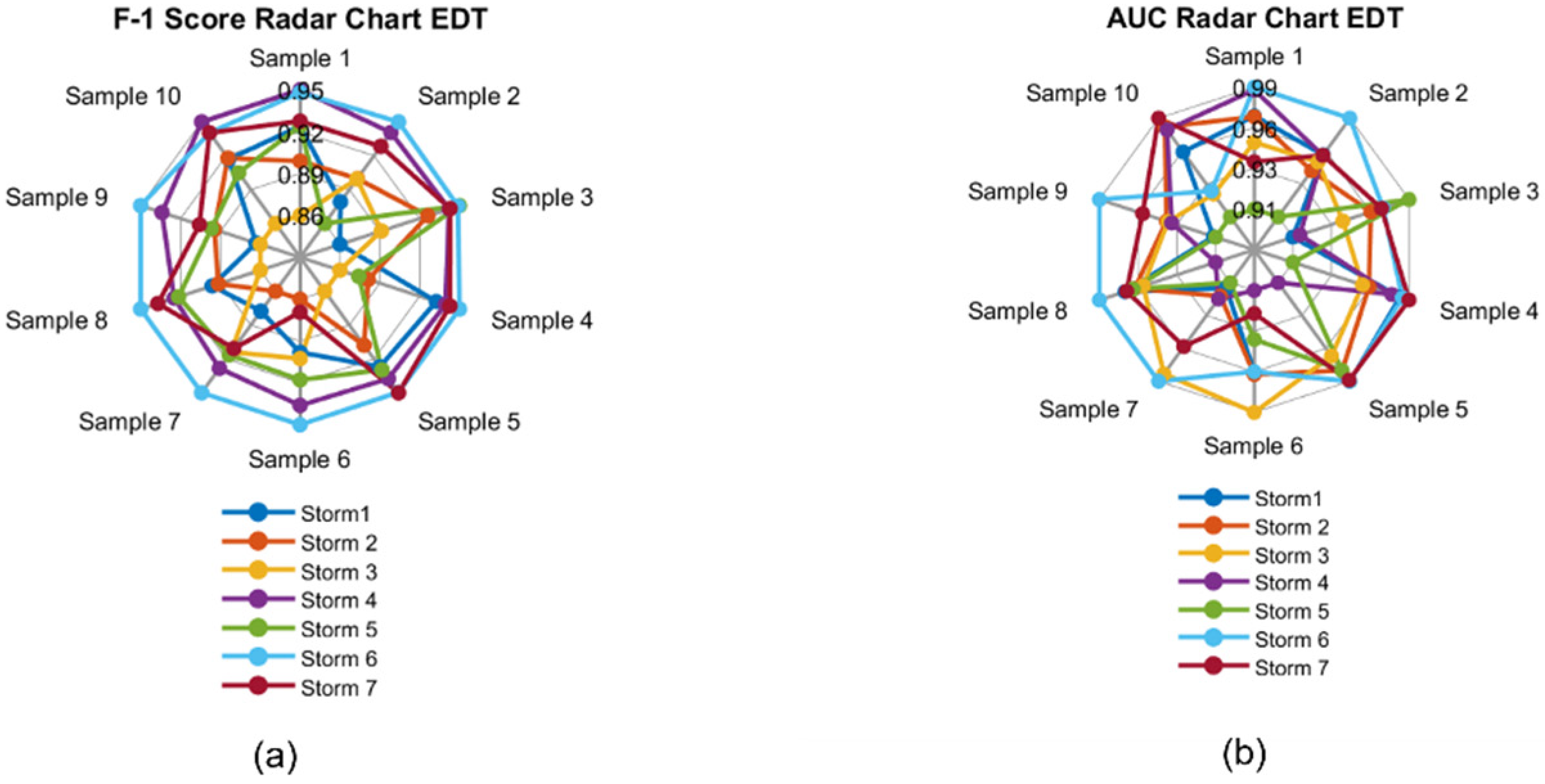
For further interpretation of the performance metrics’ values, each storm’s receiver operating characteristic (ROC) curve is presented (Figure 9). The predictability of the classifiers reports a recall or sensitivity higher than 90% at a very low FPR. Furthermore, the EDT model reports high F-1 scores and AUC values for all storms and samples selected, as explained in the “Model Training and Testing” subsection (Figure 10).
A comparison with a recent related application to the analysis of vulnerability assessment [5] was conducted to highlight the performance of the proposed two classifiers (Table 5). KNN and EDT classifiers show an improvement in the classification of highway vulnerability, with respect to the previous application across all the storm events. For the F-1 score, KNN that reported the best performance, when compared to EDT, had an average F-1 score of 0.94, with a minimum of 0.90, corresponding to storm event 3. The average F-1 score reported by [5] was 0.82, with a minimum of 0.57, corresponding to storm event 4. Similarly, the proposed classifiers showed an improvement in the AUC values (Table 6). For the AUC value, EDT that reported the best performance, when compared to EDT, had an average AUC value of 0.96, with a minimum of 0.94, corresponding to storm event 4. The average AUC value reported by [5] was 0.83, with a minimum value of 0.53, corresponding to storm event 4. The classifying capabilities of both the KNN and EDT methods outperformed the previous implementation [5] by an average of 10% across the storm events.
3.3. EDT Feature Importance Analysis
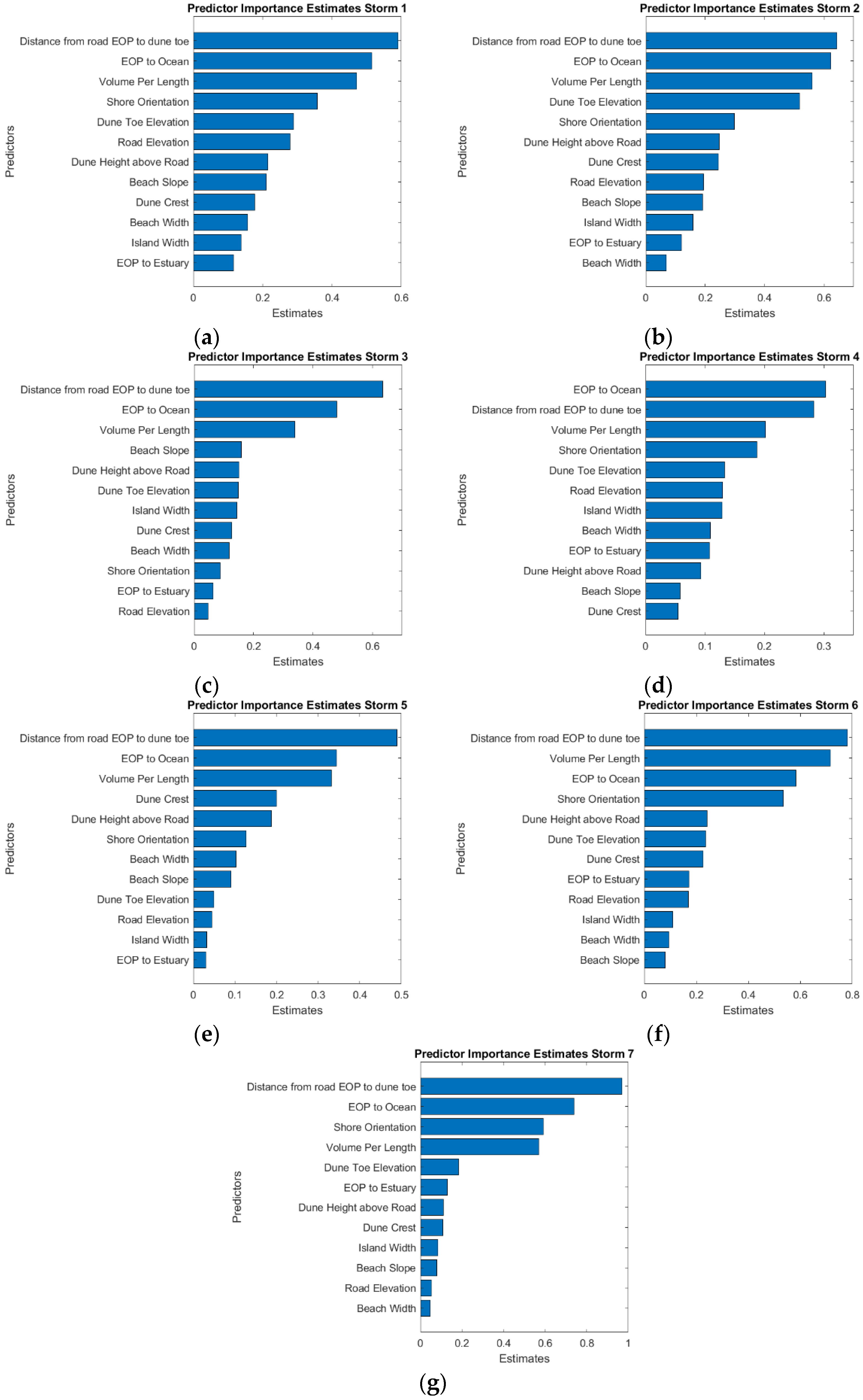
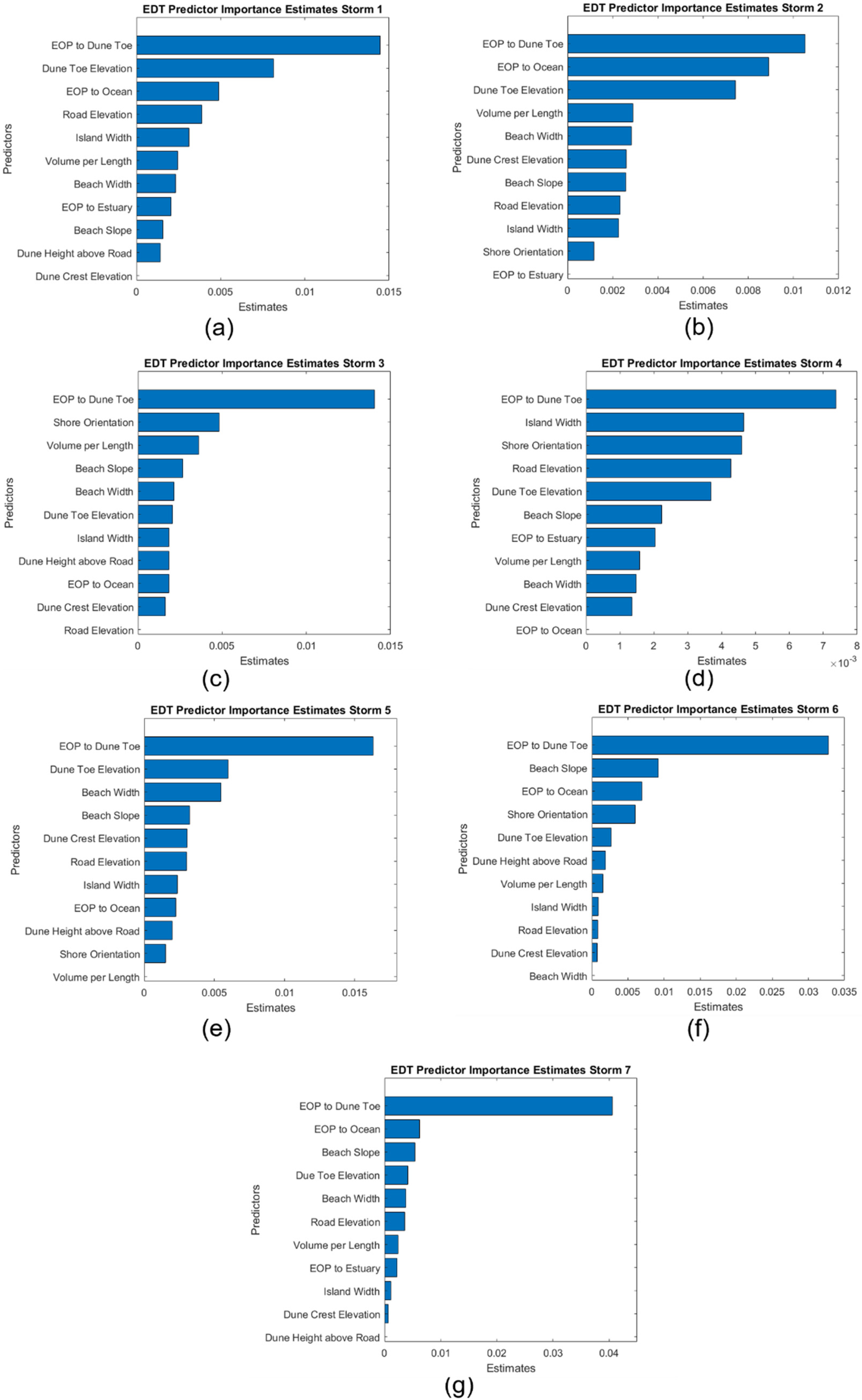
Different attributes contribute to the model with different magnitudes. For the EDT classifier, a feature importance analysis was conducted to determine how attributes affected the model performance for each of the seven storm events (Figure 11). The most important predictor across all the events is the “(11) Distance from road EOP to dune toe (ft)” (see Table 2). The second-best predictor depends on the evaluated storm. While “(5) Distance from road edge-of-pavement (EOP) to ocean shoreline (ft)” ranks second in storms 2 and 7, and the “(10) Dune toe elevation (ft) relative to NAVD 88” ranks second in storms 1 and 5. The rest of predictors that are part of the top three vary across the storm events and include “The angular difference between shore-normal orientation and the weighted mean wave direction (degrees)”, “(6) Volume above MHW between EOP and ocean shoreline (ft3/ft)”, “(1) Island Width (ft)”, “(8) Beach Width (ft)”, and “ (9) Beach Slope”.
4. Discussion
The results of coastal highway vulnerability studies inform decisions regarding when and where to implement projects. Examples of projects that could be informed by highway vulnerability studies include highway realignment, artificial dune construction, shoreline hardening, bridge construction, and regular maintenance. Maximizing the accuracy of vulnerability assessment is crucial for assuring the effectiveness of these projects and making the most out of limited transportation budgets.
A previous study [5] sought to evaluate geomorphological indicators and determine whether a weighted linear function of multiple indicators could improve the prediction of highway vulnerability, beyond that of individual indicators. Ref. [5] (2022) found that combining multiple indicators, namely the distance from road EOP to dune toe and dune toe elevation, did improve performance. However, it was not clear whether the attained accuracy (F1 score and PR AUC) was limited by the assumed function form, and there were open questions regarding whether more complex function form or machine learning methods could improve the performance.
This present study supported the hypothesis that machine learning methods would improve the classification of highway vulnerability as impacted or not. This study also affirmed the finding of [5], i.e., that distance from EOP to dune toe is a powerful and reliable predictor of highway vulnerability. Distance from EOP to dune toe was found, in this study, to be the most important predictor among most of seven storms of varying intensity and approach, relative to the study area. Some of the results seemed counterintuitive, such as the finding that dune crest elevation is not important for certain storms (Figure 6 and Figure 10). However, this area is highly managed, as discussed in [4], with frequent dune rebuilding. This may lead to dunes with relatively high crest elevations being quite close to the shoreline, where the dune is essentially a high, narrow barrier between storm waves and the roadway. In this situation, a high dune crest does not substantially lessen vulnerability.
Other factors, such as the angular difference between the shore-normal orientation and weighted mean wave direction, are shown to be important for some storms but not others. With regard to this angular difference, the relative angle between waves and structures has been shown to lead to complex effects by [39,40,41,42,43]. The research performed by [39] examined low-crested structures under an oblique wave attack. It was found that, for smooth (asphalt) structures, there was a strong dependency between the transmission coefficient and angle of wave attack, with the transmission decreasing with increasing incident wave angles. The stability of placed block revetments under oblique wave attack was investigated by [40], with the results showing that waves induce a pressure difference across the cover layer that is more complicated than that of perpendicular wave attack. Ref. [41] examined an oblique wave attack on open granular (sand) filters underneath armored slopes via physical model tests, showing that, for larger wave angles (where 0 degrees is perpendicular), the amount of filter erosion decreases. The effect of wave structure angles for tsunami loads on bridges was examined by [42,43], with the findings including the result that complex three-dimensional effects are generated by the interaction of the waves and structure. Ref. [44] examined the wave-structure interactions on bridge decks with varying geometries, also finding that loading is complex. Although these studies were not focused on ground-based roadways, similar complexity could be contributing to the results, showing the angular difference to be important for specific storms, while not as influential for others, and presenting an opportunity for further study.
While this research investigated 12 geomorphological factors that were applicable to the study area, there are other parameters cited in the literature that may be useful indicators for vulnerability assessments of roadways in other locations. A previous work [14] found that the width of elevated coastal decks affects the hydrodynamic loads imparted by waves on the structure, as well as that the ratio of “wavelength-to-deck width” is a critical factor. In the region of the present study, the roadway width did not significantly vary along the study area; therefore, this factor could not be examined. Similarly, dune vegetation was not included in this study. Past work [45,46,47,48] has shown that vegetation impacts wave-induced pressures, loads, and erosion on dunes and other structures. The fact that vegetation on dunes enhances their resiliency and dunes generally serve as protection for roadways on their landward side suggests that vegetation could have a significant effect on the vulnerability of coastal roadways. This factor was not included in the vulnerability classification models of this current study because it was difficult to adequately quantify vegetation density along a transect cross-section. In is noted that, for this specific study area, the sections that had more dense vegetation between the road and shoreline, which also had a large distance from roadway EOP to dune toe and/or roadway EOP to shoreline—this would lead to a high correlation of these variables. These two factors (roadway width and dune vegetation) could be crucial indicators in classifying roadway vulnerability for other study areas, where there may be substantial spatial variation not captured by other indicators. The study area extent was a limitation for the current research, which hindered our ability to more comprehensively assess additional vulnerability indicators. Future research could add data sets from other barrier islands, where additional variables, such as vegetation and roadway properties, could be included in the model to potentially improve the vulnerability assessment.
It is noted that the most important feature for both classifiers used in this study, distance from EOP to dune toe, can also be measured without digital computation, using aerial photographs. The development of the presented study allows researchers and practitioners to classify road vulnerability as impacted or not, based on local geomorphological observations. The models’ performance outperforms previous works significantly and can be applied to different locations where these features are available. Distance from EOP to ocean shoreline has been previously employed to evaluate highway vulnerability in this study area [4], as have long-term erosion rates and deterministic numerical modeling [49]. However, the results of this study indicate that coastal managers may be able to employ data-driven models to evaluate variability in coastal highway vulnerability on barrier islands. As remote sensing technology improves, and frequently updated topography becomes available [50,51], having a data-driven model that will classify portions of the roadway as vulnerable, without the high computational cost of deterministic numerical modeling, will be beneficial. The success of EDT in this study implies that this machine-learning model may be a useful tool for highway vulnerability studies. The model could be run with the most up-to-date geomorphology data available, in order to provide predictions regarding barrier island highway locations that are most susceptible to storm impacts. The application of the models used in this study are limited to the vulnerability classification of land-lying roadways located on wave-dominated barrier islands with sandy coastlines. Additionally, the models may not perform well for study regions where vegetated dunes are not well-correlated to distance from EOP to dune toe because vegetation was not included as a distinct variable within the model. The long-term effects of sea-level rise may bias the performance of the models, unless elevation datums are adjusted over time.
Supplementary Materials
The following supporting information can be downloaded at: https://www.mdpi.com/article/10.3390/jmse10081158/s1. Supplemental data include the correlation matrices of storm events 2 to 7.
Author Contributions
Conceptualization, E.S., A.B., and J.E.P.; methodology, J.E.P.; validation, J.E.P.; formal analysis, J.E.P.; investigation, J.E.P.; resources, E.S. and A.B.; data curation, J.E.P.; writing—original draft preparation, J.E.P. and A.B.; writing—review and editing, E.S., A.B., and J.E.P.; visualization, J.E.P. and A.B.; supervision, E.S.; project administration, E.S. All authors have read and agreed to the published version of the manuscript.
Funding
This research received no external funding. Development of the original dataset employed in this research was funded by NC Department of Transportation, research project RP 2020-46. Any opinions, findings, conclusions, or recommendations expressed in this material are those of the authors and do not necessarily reflect the views of the NC DOT, University of Illinois Urbana-Champaign, or North Carolina State University. This paper does not constitute a standard, specification, or regulation.
Institutional Review Board Statement
Not applicable.
Informed Consent Statement
Not applicable.
Data Availability Statement
Original code can be found at https://github.com/jorgeps86, accessed on 18 August 2022. Data can be provided upon reasonable request to the corresponding author.
Acknowledgments
The authors would like to thank Emily Berglund for facilitating the connections that led to this research. The contributions of four anonymous reviewers, as well as the academic editors, are appreciated and helped improve this manuscript.
Conflicts of Interest
The authors declare no conflict of interest.
References
- Daniel, J.S.; Jacobs, J.M.; Douglas, E.; Mallick, R.B.; Hayhoe, K. Impact of climate change on pavement performance: Preliminary lessons learned through the infrastructure and climate network (ICNet). In Climatic Effects on Pavement and Geotechnical Infrastructure; ASCE: Reston, VA, USA, 2014; pp. 1–9. [Google Scholar]
- Office for Coastal Management, NOAA. Hurricane Costs. 25 May 2022. Available online: https://coast.noaa.gov/states/fast-facts/hurricane-costs.html (accessed on 26 May 2022).
- NCDOT. Maintenance Operations and Performance Analysis Report (MOPAR) (31 December 2020). Asset Management NCDOT. Connect NCDOT. Available online: https://connect.ncdot.gov/resources/Asset-Management/Pages/default.aspx (accessed on 26 May 2022).
- Velásquez-Montoya, L.; Sciaudone, E.J.; Smyre, E.; Overton, M.F. Vulnerability indicators for coastal roadways based on barrier island morphology and shoreline change predictions. Nat. Hazards Rev. 2021, 22, 04021003. [Google Scholar] [CrossRef]
- Behr, A.; Berglund, E.; Sciaudone, E. Effectiveness of indicators for assessing the vulnerability of barrier island highways. Transp. Res. Part D Transp. Environ. 2022, 105, 103234. [Google Scholar] [CrossRef]
- Helderop, E.; Grubesic, T.H. Hurricane storm surge in Volusia County, Florida: Evidence of a tipping point for infrastructure damage. Disasters 2019, 43, 157–180. [Google Scholar] [CrossRef] [PubMed]
- Neumann, J.E.; Emanuel, K.; Ravela, S.; Ludwig, L.; Kirshen, P.; Bosma, K.; Martinich, J. Joint effects of storm surge and sea-level rise on US Coasts: New economic estimates of impacts, adaptation, and benefits of mitigation policy. Clim. Chang. 2015, 129, 337–349. [Google Scholar] [CrossRef] [Green Version]
- Pennison, G.P.; Cloutier, R.J.; Webb, B.M. Local Coastal Roads–Next Generation. In Proceedings of the IIE Annual Conference Proceedings, Norcross, GA, USA, 19–22 May 2018; pp. 943–948. Available online: https://www.proquest.com/scholarly-journals/local-coastal-roads-next-generation/docview/2553578393/se-2?accountid=1455 (accessed on 11 March 2022).
- Gutierrez, B.T.; Plant, N.G.; Thieler, E.R.; Turecek, A. Using a Bayesian network to predict barrier island geomorphologic characteristics. J. Geophys. Res. Earth Surface 2015, 120, 2452–2475. [Google Scholar] [CrossRef] [Green Version]
- Enwright, N.M.; Wang, L.; Wang, H.; Osland, M.J.; Feher, L.C.; Borchert, S.M.; Day, R.H. Modeling barrier island habitats using landscape position information. Remote Sens. 2019, 11, 976. [Google Scholar] [CrossRef] [Green Version]
- Talukdar, S.; Singha, P.; Mahato, S.; Shahfahad; Pal, S.; Liou, Y.-A.; Rahman, A. Land-Use Land-Cover Classification by Machine Learning Classifiers for Satellite Observations—A Review. Remote Sens. 2020, 12, 1135. [Google Scholar] [CrossRef] [Green Version]
- Wang, J.; Bretz, M.; Dewan, M.A.A.; Delvar, M.A. Machine learning in modelling land-use and land cover-change (LULCC): Current status, challenges and prospects. Sci. Total Environ. 2022, 822, 153559. [Google Scholar] [CrossRef]
- Angalakudati, M.; Calzada, J.; Farias, V.; Gonynor, J.; Monsch, M.; Papush, A.; Williams, J. Improving emergency storm planning using machine learning. In Proceedings of the 2014 IEEE PES T&D Conference and Exposition, Chicago, IL, USA, 14–17 April 2014; pp. 1–6. [Google Scholar]
- Yang, F.; Wanik, D.W.; Cerrai, D.; Bhuiyan, M.A.E.; Anagnostou, E.N. Quantifying Uncertainty in Machine Learning-Based Power Outage Prediction Model Training: A Tool for Sustainable Storm Restoration. Sustainability 2020, 12, 1525. [Google Scholar] [CrossRef] [Green Version]
- Lee, J.-W.; Irish, J.L.; Bensi, M.T.; Marcy, D.C. Rapid prediction of peak storm surge from tropical cyclone track time series using machine learning. Coast. Eng. 2021, 170, 104024. [Google Scholar] [CrossRef]
- Harvey, J.; Kumar, S.; Bao, S. Machine Learning-Based Models for Assessing Impacts Before, During and After Hurricane Florence. In Proceedings of the 2019 IEEE Symposium Series on Computational Intelligence (SSCI), Xiamen, China, 6–9 December 2019; pp. 714–721. [Google Scholar] [CrossRef]
- Fan, C.; Wu, F.; Mostafavi, A. A Hybrid Machine Learning Pipeline for Automated Mapping of Events and Locations From Social Media in Disasters. IEEE Access 2020, 8, 10478–10490. [Google Scholar] [CrossRef]
- Devaraj, A.; Murthy, D.; Dontula, A. Machine-learning methods for identifying social media-based requests for urgent help during hurricanes. Int. J. Disaster Risk Reduct. 2020, 51, 101757. [Google Scholar] [CrossRef]
- Claudino-Sales, V.; Wang, P.; Horwitz, M.H. Factors controlling the survival of coastal dunes during multiple hurricane impacts in 2004 and 2005: Santa Rosa barrier island, Florida. Geomorphology 2008, 95, 295–315. [Google Scholar] [CrossRef]
- Beuzen, T.; Harley, M.D.; Splinter, K.D.; Turner, I.L. Controls of Variability in Berm and Dune Storm Erosion. JGR Earth Surf. 2019, 124, 2647–2665. [Google Scholar] [CrossRef]
- Dolan RO BE, R.T.; Hayden, B.P.; May, P.; May, S. The reliability of shoreline change measurements from aerial photographs. Shore Beach 1980, 48, 22–29. [Google Scholar]
- National Oceanic and Atmospheric Administration (NOAA). Online Vertical Datum Transformation (VDatum). 2022. Available online: https://vdatum.noaa.gov/vdatumweb/ (accessed on 16 July 2022).
- Ortiz, A.C.; Roy, S.; Edmonds, D.A. Land loss by pond expansion on the Mississippi River Delta Plain. Geophys. Res. Lett. 2017, 44, 3635–3642. [Google Scholar] [CrossRef]
- Doran, K.S.; Long, J.W.; Overbeck, J.R. A Method for Determining Average Beach Slope and Beach Slope Variability for US Sandy Coastlines; US Department of the Interior, US Geological Survey: Reston, VA, USA, 2015. [Google Scholar]
- Zhang, Z. Introduction to machine learning: K-nearest neighbors. Ann. Transl. Med. 2016, 4, 218. [Google Scholar] [CrossRef] [Green Version]
- Freund, Y.; Schapire, R.E. Experiments with a new boosting algorithm. ICML 1996, 96, 148–156. [Google Scholar]
- Mounce, S.R.; Ellis, K.; Edwards, J.M.; Speight, V.L.; Jakomis, N.; Boxall, J.B. Ensemble decision tree models using RUSBoost for estimating risk of iron failure in drinking water distribution systems. Water Resour. Manag. 2017, 31, 1575–1589. [Google Scholar] [CrossRef] [Green Version]
- Winkler, D.; Haltmeier, M.; Kleidorfer, M.; Rauch, W.; Tscheikner-Gratl, F. Pipe failure modelling for water distribution networks using boosted decision trees. Struct. Infrastruct. Eng. 2018, 14, 1402–1411. [Google Scholar] [CrossRef] [Green Version]
- Fasaee MA, K.; Pesantez, J.; Pieper, K.J.; Ling, E.; Benham, B.; Edwards, M.; Berglund, E. Developing Early Warning Systems to Predict Water Lead Levels in Tap Water for Private Systems. Water Res. 2022, 221, 118787. [Google Scholar] [CrossRef] [PubMed]
- Guyon, I.; Elisseeff, A. An introduction to variable and feature selection. J. Mach. Learn. Res. 2003, 3, 1157–1182. [Google Scholar]
- Gelbart, M.A.; Snoek, J.; Adams, R.P. Bayesian optimization with unknown constraints. arXiv 2014, arXiv:1403.5607. [Google Scholar]
- Yang, L.; Shami, A. On hyperparameter optimization of machine learning algorithms: Theory and practice. Neurocomputing 2020, 415, 295–316. [Google Scholar] [CrossRef]
- Pesantez, J.E.; Berglund, E.Z.; Kaza, N. Smart meters data for modeling and forecasting water demand at the user-level. Environ. Model. Softw. 2020, 125, 104633. [Google Scholar] [CrossRef]
- Zhou, X.; Lu, P.; Zheng, Z.; Tolliver, D.; Keramati, A. Accident prediction accuracy assessment for highway-rail grade crossings using random forest algorithm compared with decision tree. Reliab. Eng. Syst. Saf. 2020, 200, 106931. [Google Scholar] [CrossRef]
- Rokach, L. Ensemble-based classifiers. Artif. Intell. Rev. 2010, 33, 1–39. [Google Scholar] [CrossRef]
- Breiman, L. Random forests. Mach. Learn. 2001, 45, 5–32. [Google Scholar] [CrossRef] [Green Version]
- Friedman, J.; Hastie, T.; Tibshirani, R. Additive logistic regression: A statistical view of boosting (with discussion and a rejoinder by the authors). Ann. Stat. 2000, 28, 337–407. [Google Scholar] [CrossRef]
- Gaudreault, J.G.; Branco, P.; Gama, J. An Analysis of Performance Metrics for Imbalanced Classification. In Discovery Science, Proceedings of the International Conference on Discovery Science, Halifax, NS, Canada, 11–13 October 2021; Springer: Cham, Switzerland, 2021; pp. 67–77. [Google Scholar]
- Van der Meer, J.W.; Briganti, R.; Zanuttigh, B.; Wang, B. Wave transmission and reflection at low-crested structures: Design formulae, oblique wave attack and spectral change. Coast. Eng. 2005, 52, 915–929. [Google Scholar] [CrossRef]
- Breteler, M.K.; Bezuijen, A.; Provoost, Y. Influence of oblique wave attack on stability of placed block revetments. In Coastal Engineering 2008; McKee Smith, J., Ed.; World Scientific: Hackensack, NJ, USA, 2009; Volume 4, pp. 3032–3057. [Google Scholar]
- Van Gent, M.R.A.; Wolters, G. Effects of storm duration and oblique wave attack on open filters underneath rock armoured slopes. Coast. Eng. 2018, 135, 55–65. [Google Scholar] [CrossRef]
- Istrati, D.; Buckle, I.G. Tsunami Loads on Straight and Skewed Bridges-Part 1: Experimental Investigation and Design Recommendations; Report Prepared for Oregon Dept. of Transportation & Federal Highway Administration; Oregon Dept. of Transportation: Salem, OR, USA, 2021; 193p + appx. [Google Scholar]
- Istrati, D.; Buckle, I.G. Tsunami Loads on Straight and Skewed Bridges-Part 2: Numerical Investigation and Design Recommendations; Report Prepared for Oregon Dept. of Transportation & Federal Highway Administration; Oregon Dept. of Transportation: Salem, OR, USA, 2021; 88p. [Google Scholar]
- Xiang, T.; Istrati, D. Assessment of extreme wave impact on coastal decks with different geometries via the arbitrary Lagrangian-Eulerian method. J. Mar. Sci. Eng. 2021, 9, 1342. [Google Scholar] [CrossRef]
- Coops, H.; Geilen, N.; Verheij, H.J.; Boeters, R.; van der Velde, G. Interactions between waves, bank erosion and emergent vegetation: An experimental study in a wave tank. Aquat. Bot. 1996, 53, 187–198. [Google Scholar] [CrossRef] [Green Version]
- Vuik, V.; Jonkman, S.N.; Borsje, B.W.; Suzuki, T. Nature-based flood protection: The efficiency of vegetated foreshores for reducing wave loads on coastal dikes. Coast. Eng. 2016, 116, 42–56. [Google Scholar] [CrossRef] [Green Version]
- Lo, V.B.; Bouma, T.J.; van Belzen, J.; Van Colen, C.; Airoldi, L. Interactive effects of vegetation and sediment properties on erosion of salt marshes in the Northern Adriatic Sea. Mar. Environ. Res. 2017, 131, 32–42. [Google Scholar] [CrossRef]
- Sundar, V.; Murali, K.; Noarayanan, L. Effect of vegetation on run-up and wall pressures due to cnoidal waves. J. Hydraul. Res. 2011, 49, 562–567. [Google Scholar] [CrossRef]
- Overton, M.F.; Fisher, J.S. NC Coastal Highway Vulnerability; Report No. FHWA/NC/2004-04; Prepared for U.S. Department of Transportation; US Dept. of Transportation: Washington, DC, USA, 2005; 88p. Available online: https://connect.ncdot.gov/projects/research/RNAProjDocs/2002-05FinalReport.pdf (accessed on 11 March 2022).
- Brodie, K.L.; Bruder, B.L.; Slocum, R.J.; Spore, N.J. Simultaneous Mapping of Coastal Topography and Bathymetry From a Lightweight Multicamera UAS. IEEE Trans. Geosci. Remote Sens. 2019, 57, 6844–6864. [Google Scholar] [CrossRef]
- Salameh, E.; Frappart, F.; Almar, R.; Baptista, P.; Heygster, G.; Lubac, B.; Raucoules, D.; Almeida, L.P.; Bergsma, E.W.J.; Capo, S.; et al. Monitoring Beach Topography and Nearshore Bathymetry Using Spaceborne Remote Sensing: A Review. Remote Sens. 2019, 11, 2212. [Google Scholar] [CrossRef] [Green Version]
Figure 1.
Map of hurricane tracks in the study dataset with year of landfall in parentheses, location of wave and water level data stations, and study area extents.
Figure 1.
Map of hurricane tracks in the study dataset with year of landfall in parentheses, location of wave and water level data stations, and study area extents.

Figure 2.
Morphological indicators used in the present study to classify the vulnerability of a coastal road. Island width (IW), edge of pavement to ocean shore (EOPOS), edge of pavement to dune toe (EOPDT), dune crest height above road (DCHAR), edge of pavement to estuary shore (EOPES), volume per length (VPL), dune toe elevation (DTE), beach slope (BS), and beach width (BW). Adapted from [5].


Figure 4.
An Ensemble of decision trees for classification.

Figure 5.
Correlation matrix for storm 1. Numbers in parentheses refer to morphological indicators described in Table 2. The rest of the correlation matrices are presented in the Supplemental Information.
Figure 5.
Correlation matrix for storm 1. Numbers in parentheses refer to morphological indicators described in Table 2. The rest of the correlation matrices are presented in the Supplemental Information.

Figure 6.
Feature selection analysis reported by the chi-square test for the seven storm events. “Distance from road EOP to dune toe” is the most important predictor for all storms (a–c,e–g), except storm 4 (d).
Figure 6.
Feature selection analysis reported by the chi-square test for the seven storm events. “Distance from road EOP to dune toe” is the most important predictor for all storms (a–c,e–g), except storm 4 (d).

Figure 7.
Average F-1 scores reported by the KNN and EDT classifiers, with their respective confidence intervals calculated by adding and subtracting one standard deviation for high and low boundaries, respectively.
Figure 7.
Average F-1 scores reported by the KNN and EDT classifiers, with their respective confidence intervals calculated by adding and subtracting one standard deviation for high and low boundaries, respectively.

Figure 8.
Average AUC values reported by the KNN and EDT classifiers, with their respective confidence intervals calculated by adding and subtracting one standard deviation for high and low boundaries, respectively.
Figure 8.
Average AUC values reported by the KNN and EDT classifiers, with their respective confidence intervals calculated by adding and subtracting one standard deviation for high and low boundaries, respectively.

Figure 9.
Area under the receiver operating characteristics (AUROC) for each storm event. Cutoff points showed that, with 10% of false positive rate (FPR), storm events 1, 2, 4, 6, and 7 reported true positive rates (TPR) higher than 90% of the time.
Figure 9.
Area under the receiver operating characteristics (AUROC) for each storm event. Cutoff points showed that, with 10% of false positive rate (FPR), storm events 1, 2, 4, 6, and 7 reported true positive rates (TPR) higher than 90% of the time.

Figure 10.
(a) F-1 score and (b) AUC values reported by the EDT model for each storm event and random sample.
Figure 10.
(a) F-1 score and (b) AUC values reported by the EDT model for each storm event and random sample.

Figure 11.
Feature importance results reported by the EDT models for all the storm events. Storms 1 to 7 correspond to the panels (a–g), respectively. The “(11) Distance from road EOP to dune toe (ft)” was the best predictor across all the storm events. (10) Dune Toe Elevation is the second-best predictor for (a) storm 1 and (e) storm 5. (5) EOP to Ocean Shore is also the second-best predictor for (b) storm 2 and (g) storm 7. Finally, (12) Shore orientation (degrees) is part of the top five predictors in storm 3 (c), 4 (d), and 6 (f).


Table 1.
Summary of storms and their impacts on the study area. Peak wave heights and water levels were obtained from the stations shown in Figure 1.
Table 1.
Summary of storms and their impacts on the study area. Peak wave heights and water levels were obtained from the stations shown in Figure 1.
| Storm # | Storm | Date and Duration | Storm Approach | Peak Wave Height (ft) | Max Water Level (ft NAVD88) | Storm Impacts to Study Area |
|---|---|---|---|---|---|---|
| 1 | Hurricane Irene | August 2011 50 h | Sound-side | 21.4 | 3.0 | Island breaches, erosive damage to the road, and overwash on road |
| 2 | Hurricane Sandy | October 2012 88 h | Ocean-side | 18.8 | 4.5 | Wide-spread overwash on road |
| 3 | Hurricane Arthur | July 2014 14 h | Sound-side | 18.5 | 1.3 | Erosive damage to pavement, overwash on road |
| 4 | Nor’easter | February 2016 55 h | N/A | 15.7 | 3.5 | Overwash on road |
| 5 | Hurricane Matthew | October 2016 153 h | Ocean-side | 17.2 | 3.3 | Overwash on road |
| 6 | Nor’easter | March 2018 148 h | N/A | 17.5 | 3.7 | Overwash on road |
| 7 | Hurricane Dorian | September 2019 47 h | Ocean-side | 21.9 | 4.6 | Overwash on road |
Table 2.
Geomorphological characteristics and units used as indicators for vulnerability classification.
Table 2.
Geomorphological characteristics and units used as indicators for vulnerability classification.
| Geomorphological Characteristic | |
|---|---|
|
|
Table 3.
KNN optimizable hyperparameters and search range.
| Hyperparameter | Search Range |
|---|---|
| Number of neighbors | |
| Distance metric | City block, Chebychev, Correlation, Cosine, Euclidean, Hamming, Jaccard, Mahalanobis, Minkowski (cubic), Spearman |
| Distance weight | Equal |
| Inverse | |
| Squared inverse | |
| Standardize data | True |
| False |
Table 4.
Confusion matrix of vulnerability. Adapted from [5].
Table 4.
Confusion matrix of vulnerability. Adapted from [5].
| Classified Vulnerable | Classified Not Vulnerable | |
|---|---|---|
| Observed vulnerable | True positives | False negatives |
| Observed not vulnerable | False positives | True negatives |
Table 5.
Comparison of the F-1 score values of classifying highway vulnerability.
| Storm | Parameter | [5] | KNN | EDT |
|---|---|---|---|---|
| 1 | F-1 Score | 0.85 | 0.93 | 0.92 |
| 2 | 0.88 | 0.92 | 0.91 | |
| 3 | 0.83 | 0.90 | 0.89 | |
| 4 | 0.57 | 0.96 | 0.96 | |
| 5 | 0.76 | 0.94 | 0.93 | |
| 6 | 0.89 | 0.97 | 0.97 | |
| 7 | 0.93 | 0.95 | 0.95 |
Table 6.
Comparison of the AUC values of classifying highway vulnerability.
| Storm | Parameter | [5] | KNN | EDT |
|---|---|---|---|---|
| 1 | AUC values | 0.91 | 0.92 | 0.97 |
| 2 | 0.85 | 0.91 | 0.97 | |
| 3 | 0.89 | 0.89 | 0.96 | |
| 4 | 0.53 | 0.81 | 0.94 | |
| 5 | 0.74 | 0.91 | 0.95 | |
| 6 | 0.94 | 0.96 | 0.99 | |
| 7 | 0.94 | 0.94 | 0.97 |
Publisher’s Note: MDPI stays neutral with regard to jurisdictional claims in published maps and institutional affiliations. |
© 2022 by the authors. Licensee MDPI, Basel, Switzerland. This article is an open access article distributed under the terms and conditions of the Creative Commons Attribution (CC BY) license (https://creativecommons.org/licenses/by/4.0/).
Share and Cite
MDPI and ACS Style
Pesantez, J.E.; Behr, A.; Sciaudone, E. Importance of Pre-Storm Morphological Factors in Determination of Coastal Highway Vulnerability. J. Mar. Sci. Eng. 2022, 10, 1158. https://doi.org/10.3390/jmse10081158
AMA Style
Pesantez JE, Behr A, Sciaudone E. Importance of Pre-Storm Morphological Factors in Determination of Coastal Highway Vulnerability. Journal of Marine Science and Engineering. 2022; 10(8):1158. https://doi.org/10.3390/jmse10081158
Chicago/Turabian StylePesantez, Jorge E., Adam Behr, and Elizabeth Sciaudone. 2022. "Importance of Pre-Storm Morphological Factors in Determination of Coastal Highway Vulnerability" Journal of Marine Science and Engineering 10, no. 8: 1158. https://doi.org/10.3390/jmse10081158
Note that from the first issue of 2016, this journal uses article numbers instead of page numbers. See further details here.