Hyperspectral Imaging Using Laser Excitation for Fast Raman and Fluorescence Hyperspectral Imaging for Sorting and Quality Control Applications

Abstract

A hyperspectral measurement system for the fast and large area measurement of Raman and fluorescence signals was developed, characterized and tested. This laser hyperspectral imaging system (Laser-HSI) can be used for sorting tasks and for continuous quality monitoring. The system uses a 532 nm Nd:YAG laser and a standard pushbroom HSI camera. Depending on the lens selected, it is possible to cover large areas (e.g., field of view (FOV) = 386 mm) or to achieve high spatial resolutions (e.g., 0.02 mm). The developed Laser-HSI was used for four exemplary experiments: (a) the measurement and classification of a mixture of sulphur and naphthalene; (b) the measurement of carotenoid distribution in a carrot slice; (c) the classification of black polymer particles; and, (d) the localization of impurities on a lead zirconate titanate (PZT) piezoelectric actuator. It could be shown that the measurement data obtained were in good agreement with reference measurements taken with a high-resolution Raman microscope. Furthermore, the suitability of the measurements for classification using machine learning algorithms was also demonstrated. The developed Laser-HSI could be used in the future for complex quality control or sorting tasks where conventional HSI systems fail.

1. Introduction

Hyperspectral imaging (HSI) technologies are increasingly being used in the fields of remote sensing [1], agriculture [2,3], pharmaceuticals [4,5], and medicine [6,7]. Example uses include analyzing nitrogen and water stress in wheat fields [8], measuring the coating thickness of tablets [9], and the in vivo detection of cancer [10].

For industrial applications, hyperspectral imaging methods are mainly used in the ultraviolet (UV), visible (VIS) and near-infrared (NIR) spectral ranges, because they are reasonably inexpensive, readily available, and ideally suited and proven for on-line or in-line quality control [11,12]. These methods allow a fast and extensive inspection of samples or continuous processes. Common HSI methods use broadband lighting for a sufficient excitation in the whole spectral range of interest, while other methods, such as laser-induced fluorescence (LIF) and Raman his, are not very common in the field of macroscopic HSI, although they are widely used for microscopic imaging [13,14,15].

LIF is a spectroscopic technology with high sensitivity, a wide dynamic range, and low detection limits [16]. It can be utilized, for example, for live cell microscopy of cells, using the high spectral resolution to increase the number of fluorophores that can be measured simultaneously [17].

Raman spectroscopy (RS) is a highly selective technology providing narrow and non-overlapping peaks of the measured sample. In contrast to near infrared spectroscopy, the signals are not interfered with by carbon or water absorption and nearly no sample pre-treatment is necessary. The main drawback of RS is the low fraction of scattered photons (typically < 0.0001%), which leads to low signal-to-noise ratios and long acquisition times. Some applications are, for example label-free imaging of cells [18] or high-resolution imaging of single-walled carbon nanotubes [19].

Fluorescence and Raman scattering are two competing effects and often occur together. Therefore, it is sometimes difficult to detect the weak Raman signals due to the high fluorescence background [20].

The aim of this paper is to use the simultaneously appearing fluorescence and Raman signals after laser excitation for chemical imaging of large surfaces in short periods of time. Because HSI for evaluation or classification tasks requires the highest possible variance in the underlying spectral data, the exact knowledge of the origin of the signals is of secondary importance. A distinction between fluorescence and Raman events is desirable but not absolutely necessary. The idea is that the technology, from here on called Laser-HSI, can be used for various applications in the field of process and food monitoring or sorting. Previous work has mainly focused on Raman imaging using NIR lasers to reduce the fluorescence background [21,22], while the focus of this work is the combination of Raman and fluorescence imaging. This is reflected mainly in the choice of the excitation laser and the imaging spectrometer used.

In this paper, the design of the Laser-HSI system is described, and the system is calibrated and characterized. Furthermore, some sample measurements are presented to illustrate possible applications in different areas.

2. Materials and Methods

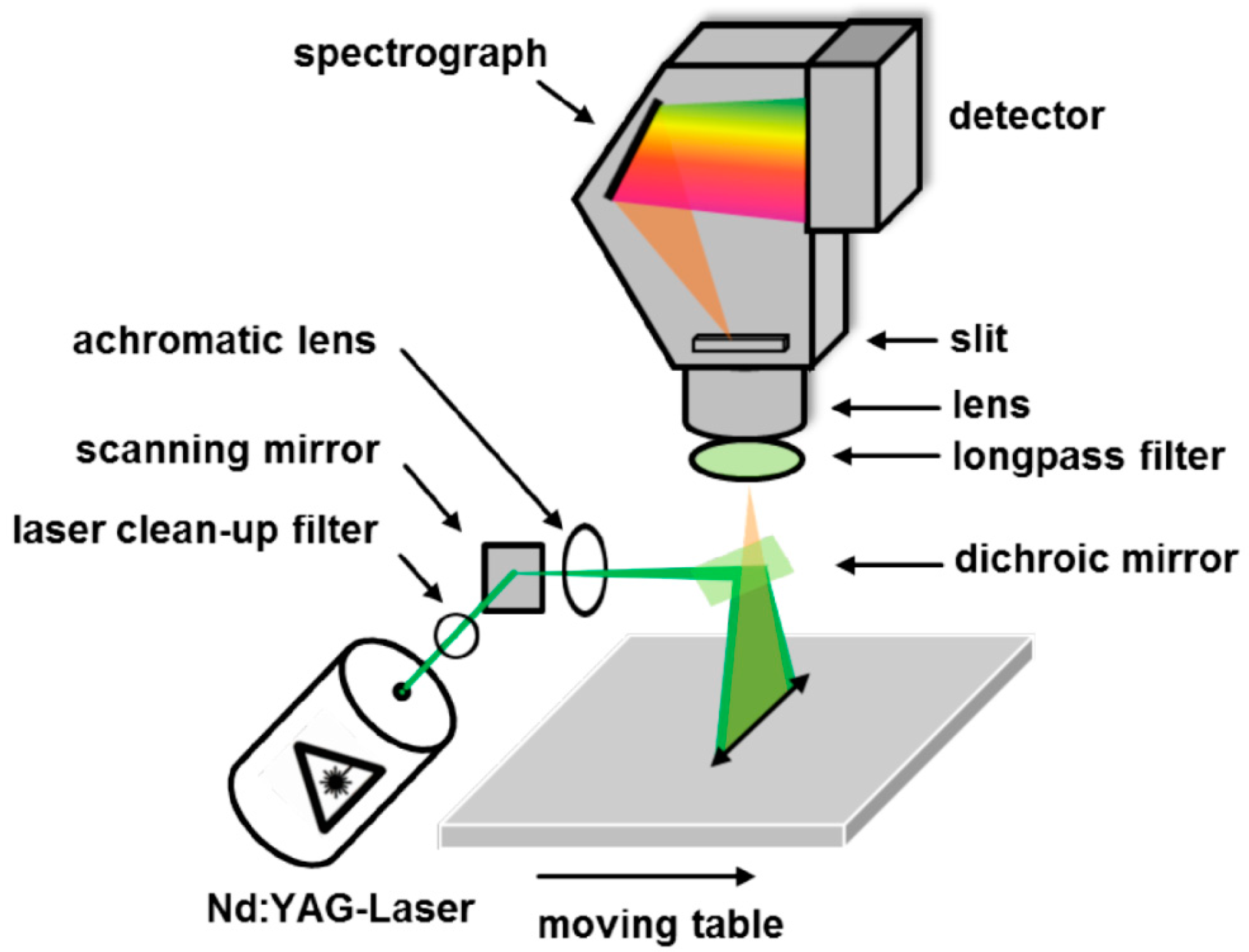
2.1. System Design and Software

The developed Laser-HSI system is schematically illustrated in Figure 1. The illumination is accomplished using a frequency-doubled Nd:YAG laser with a wavelength of 5322 nm and a maximum output power of 300 mW (GLK 32XX TS, LASOS Lasertechnik, Jena, Germany). The spectral linewidth of the laser is ≤ 1 MHz, the beam quality is M2 < 1.2, and the power stability is stated by the manufacturer as ≤±2%. The laser beam is guided through a laser clean-up filter (LL01-532, Semrock, Rochester, NY, USA), which is used to remove spontaneous emission noise. The beam then impinges a scanning mirror (dynAxis S, Scanlab, Puchheim, Germany) with variable scanning length. The scanning rate can be adjusted to the measurement task. The scanning mirror reflects the beam again and spreads the laser to form a divergent line. After passing an achromatic collimation lens with a focal length of f = 300 mm (AC508-300-A-ML, Thorlabs, Newton, MA, USA), the line passes a dichroic mirror (LPD02-532RU, Semrock, USA) with a length of 6 cm, which reflects light with a wavelength below 537 nm and allows the transmittance of light coming back from the sample with a wavelength greater than 537 nm. The dichroitic mirror is mounted at 45° to the laser plane and projects the beam to the sample surface, creating an excitation line of variable length, ranging from 0.5 cm up to 10 cm.

The hyperspectral imaging system is mounted directly above the excitation line. It consists of a holographic imaging spectrometer (Hyperspec VNIR, Headwall Photonics, Bolton, MA, USA) and a high-performance EMCCD (electron multiplying charge-coupled device) camera (Andor Luca R, Andor Technology, Belfast, UK). The spectral pixel dispersion of the imaging spectrometer is 0.7 nm. A C-mount lens is placed in front of the camera. Three different lenses were used for the experiments: two standard lenses (Cinegon 8 mm f/1.4 and Xenoplan 28 mm f/1.4, Jos. Schneider Optische Werke, Germany) and a telecentric lens with fixed working distance of 86 mm (S5LPJ2426, Sill Optics, Wendelstein, Germany) for small samples. To eliminate the excitation wavelength of the laser, a 532 nm long-pass filter is mounted before the lens (LP03-532RE, Semrock, USA).

The imaging spectrometer is built in the Offner design and optimized for a wavelength range from 400 to 1000 nm. The spectrometer can be equipped with optical slits of different widths ranging from 25 μm to 60 μm. The Si-EMCCD-detector has 1004 × 1002 pixels with a pixel size of 8 × 8 μm and 14-bit depth. The rows and columns of the sensor can be binned together up to 8× to increase the signal-to-noise ratio of the measurement, sacrificing resolution. The sensor is cooled to −20 °C and can be connected and controlled using USB. To reduce the read-out noise of the camera and to increase the signal-to-noise ratio (SNR), an electron multiplication gain between 2× and 200× can be activated.

For sample movement, a linear motion unit (VT 80, PI Micos, Eschbach, Germany) is positioned underneath the hyperspectral camera. The linear stage has a travel length of 200 mm and a step size of 0.5 μm. The whole system is housed with blackboards to minimize ambient light.

The camera, the linear motion unit, and the laser can be controlled using the imanto^®pro software package (version 3.7, Fraunhofer IWS, Dresden, Germany). This program allows the configuration of the camera, the movement of the linear motion unit, and the image acquisition, as well as the display of the live image from the camera and the current measurement. In addition, the generated spectral images can be viewed, pre-processed and saved as .envi or .hsi.jpg formats. The latter is a new data format for hyperspectral data, which includes metadata and a preview picture from the measurement in the file. Furthermore, it is possible to integrate machine learning models in the software. In this work, most data evaluation was done using Matlab^® version R2017a (Mathworks, Natick, MA, USA).

The Laser-HSI system operates as a pushbroom imager. This means that the hypercube is generated line by line and, therefore, the sample is moved underneath the camera system during the measurement using the linear motion unit. To achieve a sufficient Raman and fluorescence intensity, the imaging plane of the camera has to be aligned to the excitation laser line. Therefore, the dichroitic mirror has to be adjusted prior to the measurement.

2.2. Spectral Calibration and Spectral Resolution

The aim of the spectral calibration of the Laser-HSI is to assign correct absolute wavelength or relative Raman shifts to the rows of the detector array. For the absolute wavelength calibration, a neon lamp calibration source with characteristic emission lines between 550 nm and 750 nm (Renishaw, Wotton-under-Edge, UK) is used. The calibration source is placed underneath the camera and the spectrum is averaged 200 times using slit widths of 25, 40 and 60 μm, the Cinegon lens and no binning. For each measurement, the positions of the measured lines are used to fit a linear function between the known wavelengths of the calibration source and the row indices of the detector array. The calibration can be done automatically using an own-written Matlab^® script.

To obtain the spectral resolution of the imaging system, two sharp peaks of the neon lamp (583.4 nm and 701.6 nm) were used. In theory, these peaks should cover only one pixel of the detector. Due to the point spread function of the imaging system, the measured peaks are broadened. The resolution of the imaging system can therefore be calculated using the full width at half maximum (FWHM) of the measured peaks.

2.3. Spatial Resolution

The spatial resolution perpendicular to the measurement line depends on the speed of the moving stage and the frame-rate of the camera, and can, therefore, be easily controlled and adjusted to achieve squared pixels. The spatial resolution parallel to the measurement line depends on several factors, namely the working distance, the focal length of the used lens, and the number of detector pixels in the spatial dimension of the camera. The fixed structure of the spectrograph and camera allows the spatial resolution required for the application to be adjusted with a lens with an appropriate focal length, which simultaneously results in a certain field of view (FOV). To measure the spatial resolution, a calibration target (R2L2S1P1, Thorlabs, Newton, MA, USA) with black and white lines is placed underneath the camera and illuminated with halogen light. One line of the target is measured 200 times and averaged. The measured black and white transitions of the sample at a wavelength of 600 nm are differentiated and the FWHM of the obtained peaks is taken as the spatial resolution. The spatial resolution for the three different lenses was determined with working distances of 330 mm and 82.7 mm and FOVs of 386 mm, 104 mm and 4 mm. A slit width of 40 µm was used for the measurements.

2.4. Example Measurements

To evaluate the developed Laser-HSI, four samples from quite different fields of application were measured: (a) a mixture of sulphur and naphthalene; (b) a carrot slice; (c) black polymer particles; and, (d) a lead zirconate titanate (PZT) piezoelectric actuator with contaminations. The specific experimental conditions are shown in

Table 1. Experimental conditions.

Experiment	Lens	Laser Power (mW)	Integration Time (ms)	Speed (mm·s−1)	Frame rate (Hz)	Binning (Lateral × Spectral)	Total Time (s)	Total Area (cm2)
(a) sulphur and naphthalene	Xenoplan	150	25	2.4	24	2 × 1	20	50
(b) carrot slice	Xenoplan	300	100	0.8	8	2 × 1	50	42
(c) black polymers	Xenoplan	150	25	2.4	24	2 × 1	42	105
(d) PZT actuator	Sill	300	100	0.013	8	4 × 1	170	2.3

.

For referencing the experiments (a) and (d), a Raman microscope (inVia, Renishaw GmbH, Wotton-under-Edge, UK) with a 514.5 nm argon ion laser source was used. In case of (a), a 100× magnification lens was used and the spectra were accumulated for 10 s and measured between 150 cm⁻¹ and 3500 cm⁻¹.

In case of (d), areas with suspected contaminations were mapped using a 50× magnification lens and a spatial resolution of approximately 5 μm. The integration time was 0.1 s and the spectra were measured between 150 cm⁻¹ and 2000 cm⁻¹.

For referencing the experiment (b), the same Raman microscope with a 785 nm diode laser (to reduce fluorescence) and 50× magnification lens was used. The spectra were measured between 800 cm⁻¹ and 1800 cm⁻¹ and accumulated ten times for 1 s.

2.5. Classification Experiments

To show that the system can be used for process monitoring and sorting tasks, classification experiments were performed for the experiments (a), (c), and (d). Therefore, 500 spectra per class were selected at random and a random forest [23] model was trained using the fitcensemble function of Matlab^® using default hyperparameters. Prior to the training, a principal component analysis was conducted and only the scores of the first five principal components were used. To estimate the accuracy of the trained model, 10-fold cross validation was used and the cross-validated accuracy was used as a measure of the quality of the model. Finally, the trained model was applied to all spectra in the hyperspectral measurement to generate a classification image of the sample.

3. Results

3.1. System Design

The individual components of the Laser-HSI were selected and optimized with regard to the specific application requirements. With a wavelength of 532 nm, the frequency-doubled Nd:YAG laser used offers a good compromise between the expected intensity of the Raman scattering and the fluorescence intensity. Furthermore, the wavelength of the light emitted by the samples is in the range of the optimum quantum efficiency of the used silicon detector. If Raman measurements are made, this wavelength is particularly suitable for inorganic or weakly fluorescent samples. A near-infrared laser (e.g., 785 nm) would be more suitable for organic or highly fluorescent samples, but this would also further decrease the Raman intensity. Compared to argon ion lasers, which emit a similar wavelength, the Nd:YAG laser offers low power consumption, easy handling and a compact design, which facilitates industrial use (e.g., in recycling plants).

To generate the laser line, a scanning mirror was used. Alternatively, one could use a cylindrical or Powell lens [24] to generate the excitation line. Both approaches have advantages and disadvantages. If a cylindrical lens is used, no moving parts are required and a compact design can be achieved. On the other hand, a cylinder lens produces a non-uniform intensity distribution along the excitation line. This can be reduced by using a Powell lens, but these lenses must be optimized for a certain beam diameter and fan angle, which reduces the flexibility of the system. A disadvantage of the scanning mirror is an increased intensity at the reversal points of the mirror (at the edges of the excitation line) and the limited scanning speed, which can lead to problems using short integration times for the detector. Because the setup presented here should be as flexible as possible, a scanning mirror was used. For later industrial applications, the use of cylindrical or Powell lenses can be considered.

The used imaging spectrometer is optimized for spectroscopy in the visible and near-infrared wavelength range (400–1000 nm). Therefore, the spectral resolution is quite low for Raman spectroscopy (see Section 3.2). This has a negative effect on the usability of the device for tasks where a high spectral resolution is required. On the other hand, it is possible to measure a much larger wavelength range than with a Raman spectrometer. This could be useful for some questions; for example, when fluorescence signals are to be measured, which often extend over a wider wavelength range (see experiment (c)). In addition, the used imaging spectrometer is cheaper and more readily available then a Raman imaging spectrometer.

The EMCCD detector used enables a reduction of the readout noise due to the built-in amplification and thus enables the measurement of weak Raman and fluorescence signals. The disadvantage is the relatively low frame rate of ~12 Hz using the full detector, which can, however, be increased using binning.

The C-mount connection allows flexibility regarding the FOV and the spatial resolution of the measurement. In summary, due to the modular design of the Laser-HSI system an individual adaptation to the respectively specific measuring application is possible.

3.2. Spectral Calibration and Spectral and Spatial Resolution

The results of the spectral calibration for different slit widths are shown in

Table 2. Results of the spectral calibration of the Laser-HSI.

Slit Width (μm)	Wavelength Interval (nm)	Mean Absolute Error (nm)	FWHM (583 nm) (nm)	FWHM (702 nm) (nm)	FWHM (583 nm) (cm−1)	FWHM (702 nm) (cm−1)
25	0.79	0.25	1.8	2.0	52.9	40.6
40	0.8	0.58	2.8	3.1	82.3	63.0
60	0.79	1.28	4.1	4.5	120.5	91.4

. For all three slit widths, a similar covered wavelength range of approximately 330 nm to just over 1100 nm is obtained. A wavelength interval of about 0.8 nm per pixel is determined for all three slits. The quality of the spectral calibration can be determined from the mean absolute error of the line positions to the reference line positions. The mean absolute error is relatively small for all three measurements, but increases with wider slits. The reason for this is the decreasing spectral resolution, which leads to broader lines and makes the automated peak selection more difficult, resulting in larger calibration errors. The spectral resolution of the system was measured for the peaks at 583.4 nm and 701.6 nm, and ranges from about 2 nm for 25 μm slit width, to over 4 nm for 60 μm slit width. It can also be seen that the spectral resolution decreases slightly for larger slit widths.

Because the used spectrometer is optimized for visible and near-infrared hyperspectral imaging, the spectral resolution (in nanometers) decreases inherently due to the equidistant wavelength-resolution of the detector. In addition, it is possible to cover a much wider spectral range, from 535 nm up to 1000 nm, compared to a classic Raman spectrometer. Because of the low spectral resolution of the system, the typical calibration for Raman spectrometer, using reference substances like sulphur or naphthalene, could not be applied. Sometimes it was not possible to clearly assign the measured signals to the bands of the reference spectra. Therefore, the typical calibration could not be performed and the Raman shifts in the measurements were only calculated using the wavelengths obtained by the absolute calibration with the neon lamp calibration source.

The results for the determination of the spatial resolution for different lenses and FOVs are shown in

Table 3. Results of the spatial calibration of the Laser-HSI.

Lens	Working Distance (mm)	FOV (mm)	FWHM (pixel)	Spatial Resolution (mm)
Cinegon, f/1.4, 8 mm	330	386	3.49	1.34
Xenoplan, f/1.4, 28 mm	330	104	3.97	0.41
Sill, S5LPJ2426	85.7	4	4.18	0.02

. The measured resolutions are 1.31 mm for the Cinegon lens, 0.41 mm for the Xenoplan and 17 μm for the Sill telecentric lens with FOVs of 386 mm, 104 mm, and 4 mm, respectively. This shows the versatility of the developed laser-hyperspectral imager in terms of resolution and measurement area. It can be used to measure small samples with high resolution or to measure larger samples; e.g., in a conveyer belt application for sorting and recycling tasks. The FOV and the achievable resolution mostly depend on the used optics. Nevertheless, it has to be taken into account that with increasing FOV and working distance, more laser power is needed to maintain the signal intensity.

3.3. Example Measurements

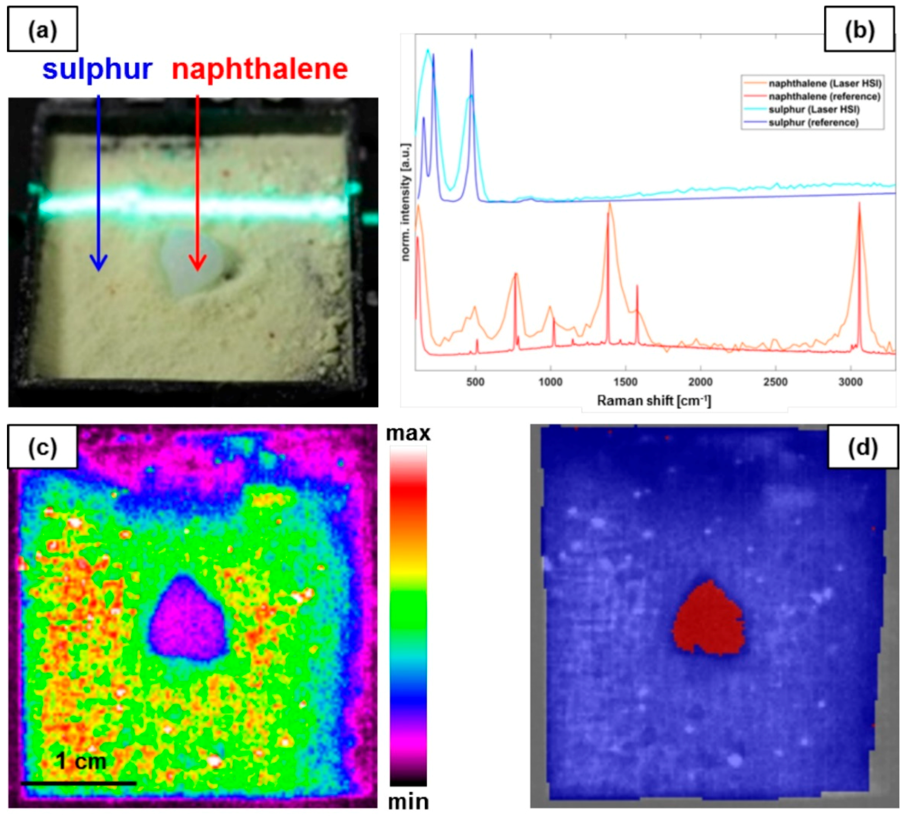
3.3.1. Spatial Distribution of Naphthalene Granules in a Sulphur Matrix (a)

A mixture of sulphur and naphthalene was measured using the Laser-HSI and the results are summarized in Figure 2. A picture of the sample (Figure 2a,c) shows a false color image of the measured intensity at ~180 cm⁻¹. At this wavenumber there is a slight overlap between the peaks of the two materials, but the intensity of sulphur is much higher than the intensity of naphthalene, so the position of the naphthalene can be clearly identified in the false color image. Despite the low resolution of the spectrograph, the characteristic peaks of both sulphur and naphthalene are clearly visible and the spectra show good agreement with reference spectra (Figure 2b). Fine spectral features like the sulphur peaks at 154 cm⁻¹ and 219 cm⁻¹ are not resolved. In addition, a precise determination of the peak position is not possible due to the low spectral resolution. Nonetheless, it is possible to determine the spatial distribution of the two materials in the sample. The measurement of the sample area of ~16 cm² only took around 20 s with a spatial resolution of approximately 0.4 mm. The acquired spectra were used to train a classification model to discriminate between sulphur and naphthalene. The resulting model has a high cross-validation accuracy of 99.9%. The classification image is shown in Figure 2d.

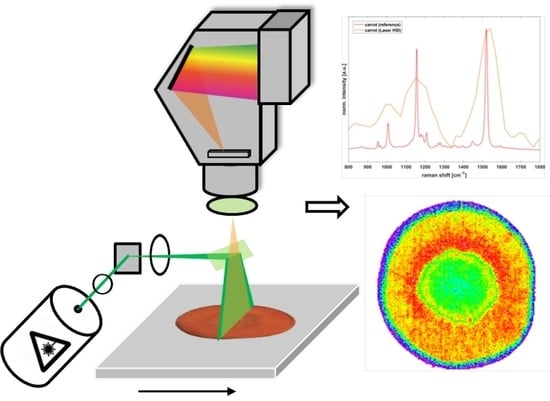
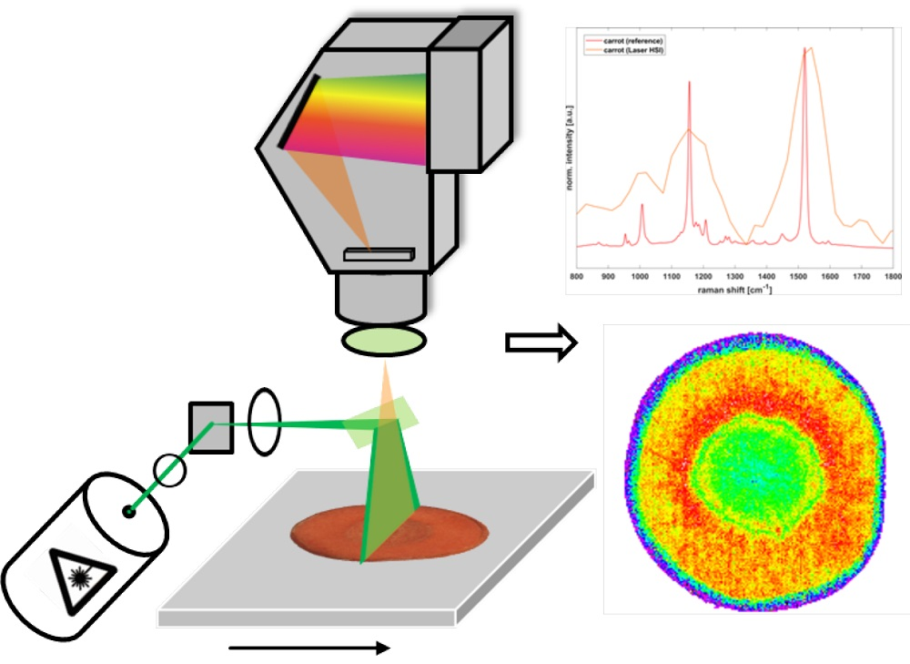
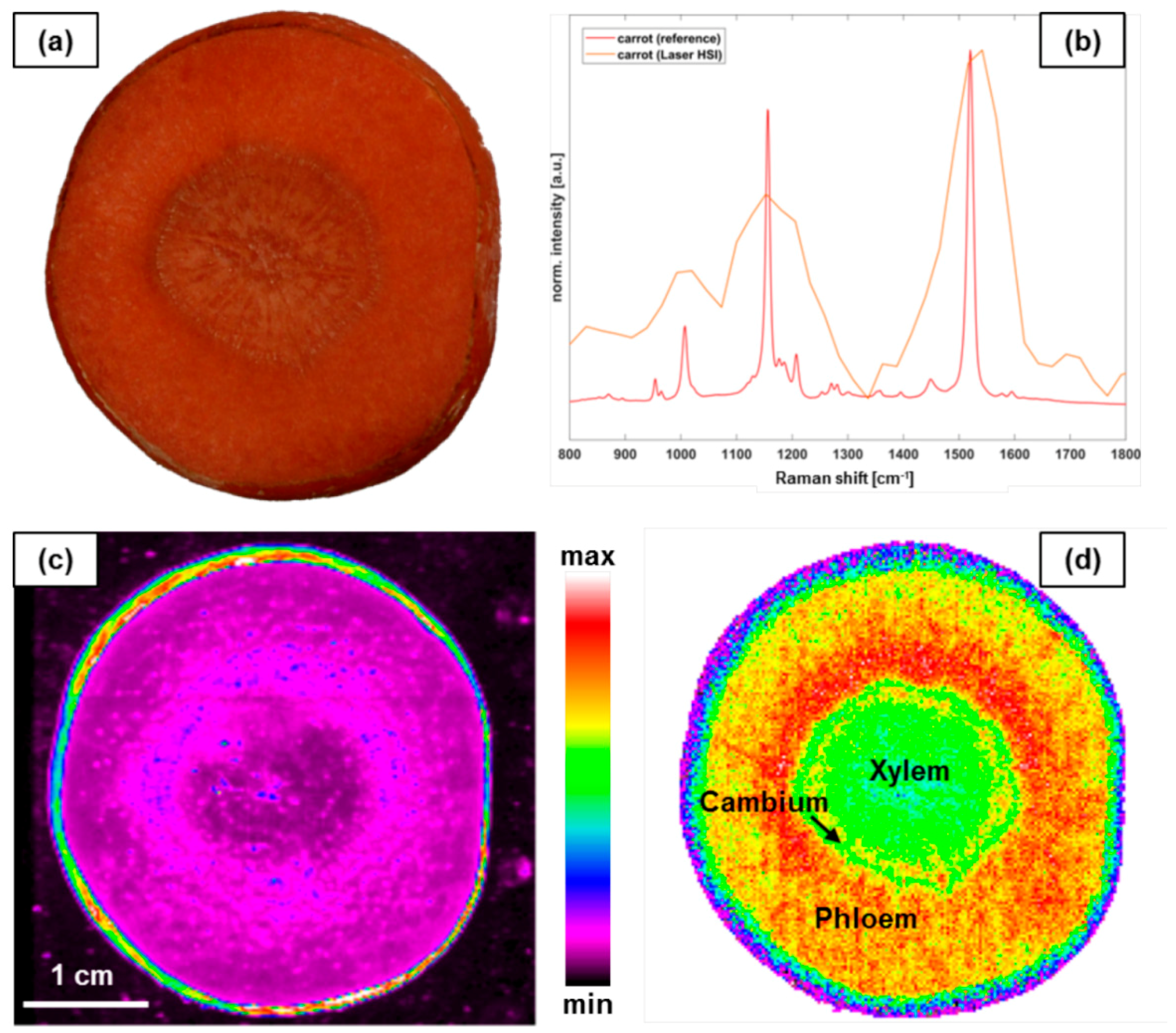
3.3.2. Carotenoid Distribution in a Carrot Slice (b)

A carrot slice was measured with the Laser-HSI and the results are shown in Figure 3. A picture of the sample (Figure 3a,c) shows a false color image of the measured intensity at ~1000 cm⁻¹ before any pre-processing. This image, therefore, shows the fluorescence of the carrot slice. Figure 3b shows an example spectrum of the carrot slice scan after fluorescence background removal with two characteristic carotenoid peaks at 1156 cm⁻¹ and 1521 cm⁻¹, which originate from C=C stretching vibrations of the carotenoids [25]. The background was removed fitting a polynomial of fourth degree to the spectra using a non-quadratic cost function [26]. The peaks are also in good agreement with the peaks from the reference spectra acquired with the Raman microscope. The intensity of the peaks is proportional to the carotenoid concentration. The band at 1521 cm⁻¹ was used to calculate the distribution of the relative carotenoid concentration (Figure 3d). The image shows an uneven distribution of the carotenoid in the carrot slice. The concentration in the xylem is relatively low and increases towards the cambium. Towards the outer areas of the slice (phloem), the concentration decreases again. This is in good agreement with previous findings and shows the potential of the Laser-HSI in the area of food surveillance, quality control, and research [25]. When comparing images Figure 3c and 3d, it can be seen that there is a correlation between the distribution of the fluorescence and the carotenoid distribution in the inner part of the slice. However, at the edge of the slice, the carotenoid concentration is very low, but a strong fluorescence can be observed. This shows that it can be useful to measure Raman and fluorescence signals at the same time to get the information with only one measurement, which could be especially useful for time-critical tasks.

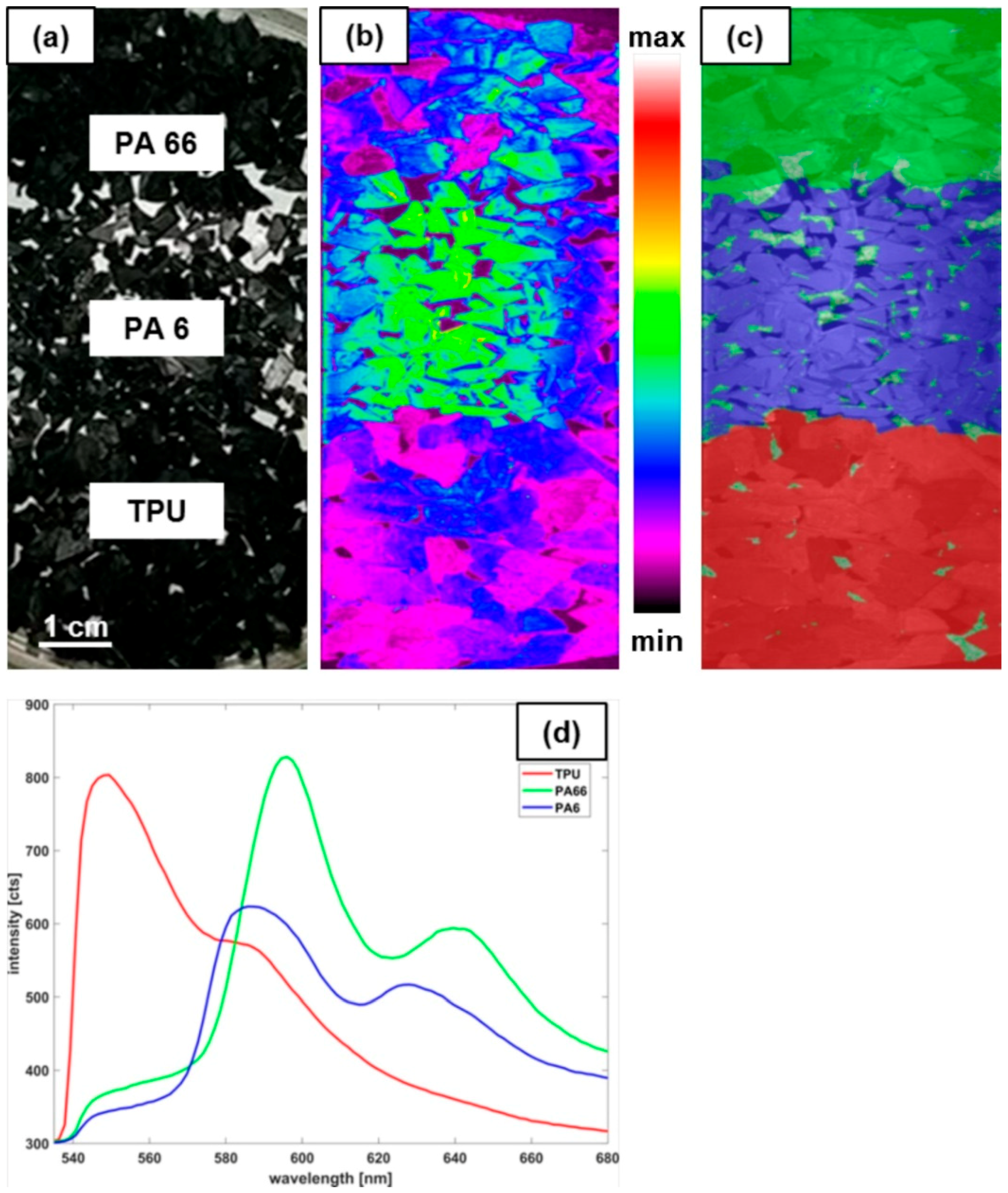
3.3.3. Black Polymer Sorting (c)

The appearance of black polymers is achieved by adding filling materials like carbon black. The recycling of black polymers to high purity recycled materials is difficult because sorting techniques fail due to the low recognition rates of common sensor techniques like near-infrared spectroscopy. Laser-HSI is a promising technology to solve this problem because many black polymers show characteristic fluorescence signals. Therefore, three different kind of black polymer particles, namely polyamide 6 (PA6), polyamide 66 (PA66), and thermoplastic polyurethane (TPU) were imaged using the Laser-HSI. A picture of the three black polymers (Figure 4a,b) shows a false color image of the measured intensity at 580 nm. Figure 4d shows some Laser-HSI example spectra of the polymers. It is evident that there are clear differences in the spectral signatures which may be used to classify and, in consequence, sort the polymer particles.

The obtained classification model for the polymers shows a cross validation accuracy of 99.6%, which is very promising for the use of the Laser-HSI for sorting black plastics for recycling. The trained model was applied to all spectra in the hyperspectral measurement to generate a classification image of the sample (Figure 4c).

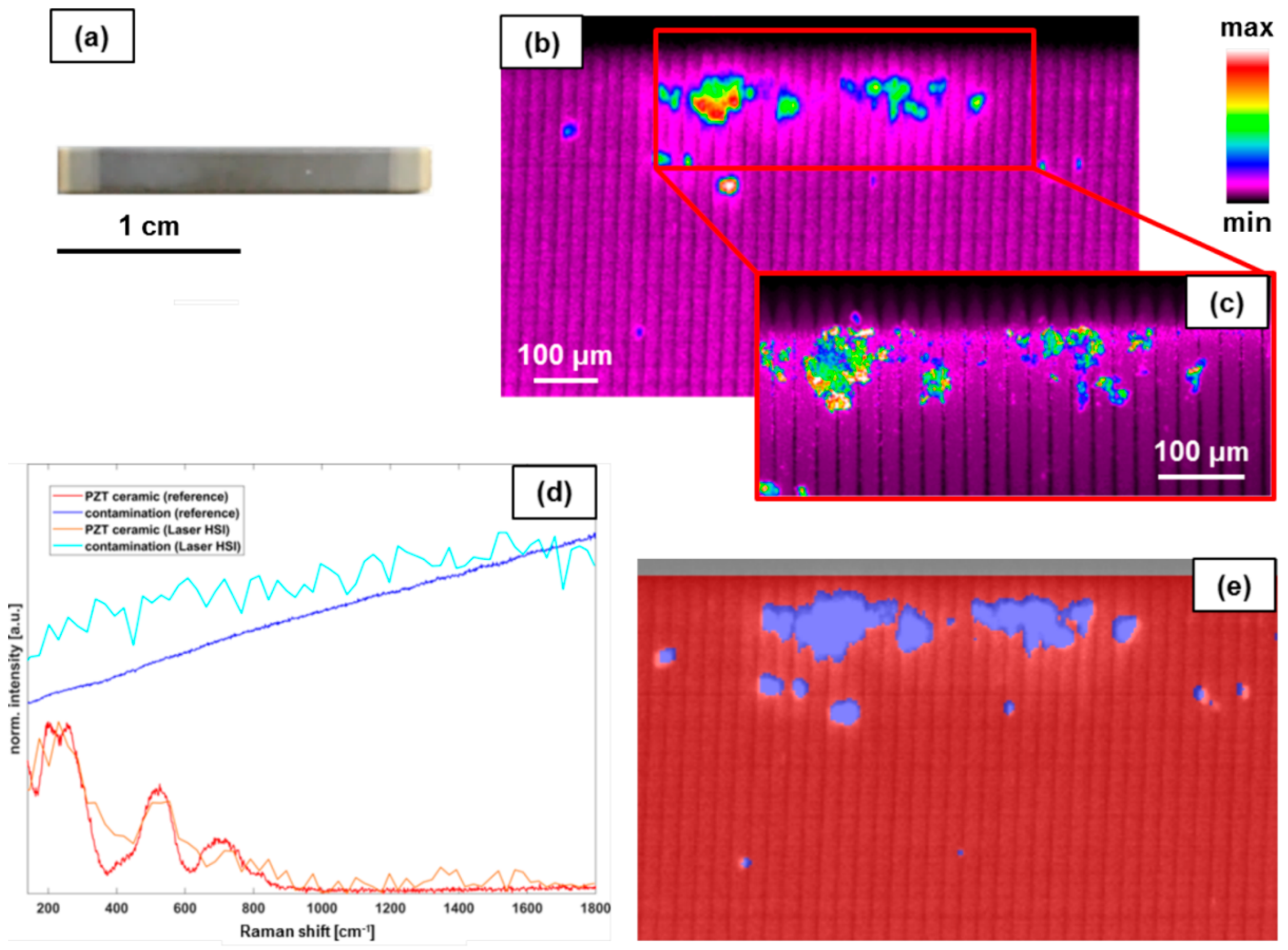
3.3.4. Contaminations on PZT Piezoelectric Actuators (d)

For the last experiment, a PZT piezoelectric actuator was investigated with a high-resolution Laser-HSI measurement. The actuator is contaminated with organic substances of unknown origin and the aim of the experiment is to locate these impurities, using the Laser-HSI. Figure 5a shows a picture of the PZT piezoelectric actuator and Figure 5b shows a section of a measurement of a contaminated sample acquired with the Laser-HSI. Figure 5c shows a section of the same area, which was measured with the Raman microscope. Both figures show a false color representation of the Raman intensity at 230 cm⁻¹. Figure 5d shows spectra of the PZT ceramic and the contamination, measured with the Laser-HSI and the Raman microscope. The PZT spectra shows the typical bands of the PZT ceramic [27]. In the areas of contamination, strong fluorescence caused by the organic impurities can be seen. The shape and dimensions of the contamination show a good agreement for both measurements. The trained classification model shows a cross validation accuracy of 100% and the classification image is shown in Figure 5e. If needed, the peaks of the PZT ceramic bands could be used to find, for example, defects in the layers of the piezoelectric actuator.

This experiment shows that the developed Laser-HSI provides equivalent results to a Raman microscope for this task. While the Laser-HSI measurement takes about three min per sample, a complete mapping with the Raman microscope would take several hours. Therefore, the Laser-HSI could be used as a fast tool for the high-resolution quality control of small components.

4. Conclusions

In this paper a fast, line-scanning hyperspectral imaging system with laser excitation using fluorescence or/and Raman scattered light for imaging analysis was introduced.

Four different application examples demonstrate the wide range of possible applications. The experiments carried out show that the described Laser-HSI system makes it possible to measure the Raman or fluorescence spectra of relatively large sample areas, with a high spatial resolution and in a relatively short amount of time. This opens up interesting application possibilities in many areas, from quality control in the food industry to surface inspection and recycling. The modular design of the system makes it possible to adapt the measuring range and spatial resolution to the problem at hand. In the experiments, measuring widths between 38 cm and 4 mm, with resolutions between 1.3 mm and 20 mm, were achieved. Furthermore, the system was spectrally calibrated and it could be shown that the spectra obtained for a number of test substances are in good agreement with literature or reference measurements. The minimal spectral resolution of approximately 1.8 nm at 583 nm is below the resolution of a conventional Raman spectrometer. On the other hand, the spectral range covered is much larger. This will be used in future attempts to obtain further information about the samples; for example, by measuring reflective properties in the spectral ranges in which no Raman or fluorescence signals are expected. Future developments will focus, in particular, on the investigation of the application for the recycling of black polymers. In addition, it will be investigated how measurements can be further accelerated. Other hyperspectral cameras and stronger lasers with different wavelengths could be used for this purpose.

5. Patents

In reference to the work presented here, two patents with the patent numbers DE102018210019.5 and DE102018210015.2 have been filed.

References

1. Borengasser, M.; Hungate, W.S. Hyperspectral Remote Sensing. Principles and Applications; CRC Press: Boca Raton, FL, USA, 2007. [Google Scholar]
2. Dale, L.M.; Thewis, A.; Boudry, C.; Rotar, I.; Dardenne, P.; Baeten, V.; Pierna, J.A.F. Hyperspectral imaging applications in agriculture and agro-food product quality and safety control: A review. Appl. Spectrosc. Rev. 2013, 48, 142–159. [Google Scholar] [CrossRef]
3. Elmasry, G.; Kamruzzaman, M.; Sun, D.W.; Allen, P. Principles and applications of hyperspectral imaging in quality evaluation of agro-food products: A review. Crit. Rev. Food Sci. Nutr. 2012, 52, 999–1023. [Google Scholar] [CrossRef] [PubMed]
4. Gowen, A.A.; O’Donnell, C.P.; Cullen, P.J.; Bell, S.E.J. Recent applications of chemical imaging to pharmaceutical process monitoring and quality control. Eur. J. Pharm. Biopharma. 2008, 69, 10–22. [Google Scholar] [CrossRef] [PubMed]
5. Gendrin, C.; Roggo, Y.; Collet, C. Pharmaceutical applications of vibrational chemical imaging and chemometrics: A review. J. Pharm. Biomed. Anal. 2008, 48, 533–553. [Google Scholar] [CrossRef] [PubMed]
6. Calin, M.A.; Parasca, S.V.; Savastru, D.; Manea, D. Hyperspectral imaging in the medical field: present and future. Appl. Spectrosc. Rev. 2013, 49, 435–447. [Google Scholar] [CrossRef]
7. Lu, G.; Fei, B. Medical hyperspectral imaging: A review. J. Biomed. Opt. 2014, 19, 10901. [Google Scholar] [CrossRef] [PubMed]
8. Tilling, A.K.; O’Leary, G.J.; Ferwerda, J.G.; Jones, S.D.; Fitzgerald, G.J.; Rodriguez, D.; Belford, R. Remote sensing of nitrogen and water stress in wheat. Field Crop. Res. 2007, 104, 77–85. [Google Scholar] [CrossRef]
9. Lewis, E.N.; Kidder, L.H.; Lee, E. NIR chemical imaging—Near infrared spectroscopy on steroids. NIR News 2005, 16, 2–4. [Google Scholar] [CrossRef]
10. Martin, M.E.; Wabuyele, M.B.; Chen, K.; Kasili, P.; Panjehpour, M.; Phan, M.; Overholt, B.; Cunningham, G.; Wilson, D.; DeNovo, R.C.; et al. Development of an Advanced Hyperspectral Imaging (HSI) System with Applications for Cancer Detection. Ann. Biomed. Eng. 2006, 34, 1061–1068. [Google Scholar] [CrossRef] [PubMed]
11. Gowen, A.; Odonell, C.; Cullen, P.; Downey, G.; Frias, J. Hyperspectral imaging—An emerging process analytical tool for food quality and safety control. Trends Food Sci. Tech. 2007, 18, 590–598. [Google Scholar] [CrossRef]
12. Boldrini, B.; Kessler, W.; Rebner, K.; Kessler, R.W. Hyperspectral imaging: A review of best practice, performance and pitfalls for in-line and on-line applications. J. Near Infrared Spec. 2012, 20, 483–508. [Google Scholar] [CrossRef]
13. Stewart, S.; Priore, R.J.; Nelson, M.P.; Treado, P.J. Raman imaging. Ann. Rev. Anal. Chem. 2012, 5, 337–360. [Google Scholar] [CrossRef] [PubMed]
14. Févotte, G. In situ Raman spectroscopy for in-line control of pharmaceutical crystallization and solids elaboration processes: A review. Chem. Eng. Res. Des. 2007, 85, 906–920. [Google Scholar] [CrossRef]
15. Adar, F.; Geiger, R.; Noonan, J. Raman spectroscopy for process/quality control. Appl. Spectrosc. Rev. 1997, 32, 45–101. [Google Scholar] [CrossRef]
16. Lakowicz, J.R. Principles of Fluorescence Spectroscopy; Springer: New York, NY, USA, 2006. [Google Scholar]
17. Zimmermann, T.; Rietdorf, J.; Pepperkok, R. Spectral imaging and its applications in live cell microscopy. FEBS Lett. 2003, 546, 87–92. [Google Scholar] [CrossRef] [Green Version]
18. El-Mashtoly, S.F.; Petersen, D.; Yosef, H.K.; Mosig, A.; Reinacher-Schick, A.; Kötting, C.; Gerwert, K. Label-free imaging of drug distribution and metabolism in colon cancer cells by Raman microscopy. Analyst 2014, 139, 1155–1161. [Google Scholar] [CrossRef] [PubMed]
19. Hartschuh, A.; Sánchez, E.J.; Xie, X.S.; Novotny, L. High-resolution near-field Raman microscopy of single-walled carbon nanotubes. Phys. Rev. Lett. 2003, 90, 95503. [Google Scholar] [CrossRef] [PubMed]
20. McCreery, R.L. Raman Spectroscopy for Chemical Analysis; Wiley: New York, NY, USA, 2000. [Google Scholar]
21. Qin, J.; Chao, K.; Kim, M.S. High-throughput Raman chemical imaging for evaluating food safety and quality. In Proceedings of the Sensing for Agriculture and Food Quality and Safety VI, San Francisco, CA, USA, 1–6 February 2014; p. 91080F. [Google Scholar]
22. Qin, J.; Kim, M.S.; Chao, K.; Schmidt, W.F.; Cho, B.K.; Delwiche, S.R. Line-scan Raman imaging and spectroscopy platform for surface and subsurface evaluation of food safety and quality. J. Food Eng. 2017, 198, 17–27. [Google Scholar] [CrossRef]
23. Breiman, L. Random forests. Mach. Learn. 2001, 45, 5–32. [Google Scholar] [CrossRef]
24. Palonpon, A.F.; Ando, J.; Yamakoshi, H.; Dodo, K.; Sodeoka, M.; Kawata, S.; Fujita, K. Raman and SERS microscopy for molecular imaging of live cells. Nat. Protoc. 2013, 8, 677–692. [Google Scholar] [CrossRef] [PubMed]
25. Baranska, M.; Baranski, R.; Schulz, H.; Nothnagel, T. Tissue-specific accumulation of carotenoids in carrot roots. Planta 2006, 224, 1028–1037. [Google Scholar] [CrossRef] [PubMed]
26. Mazet, V.; Carteret, C.; Brie, D.; Idier, J.; Humbert, B. Background removal from spectra by designing and minimising a non-quadratic cost function. Chemometr. Intell. Lab. 2005, 76, 121–133. [Google Scholar] [CrossRef]
27. Camargo, E.R.; Frantti, J.; Kakihana, M. Low-temperature chemical synthesis of lead zirconate titanate (PZT) powders free from halides and organics. J. Mater. Chem. 2001, 11, 1875–1879. [Google Scholar] [CrossRef]
Figure 1. Schematic illustration of the developed laser hyperspectral imaging system (Laser-HSI) system.
Jimaging 04 00110 g001
Figure 2. Laser-HSI of mixture of sulphur and naphthalene. (a) Picture of the sample with laser excitation line. (b) Normalized example spectra of sulphur and naphthalene with reference spectra acquired with the Raman microscope. (c) False color image of the measured intensity at ~180 cm−1 (sulphur). (d) Results of the Laser-HSI classification (blue = sulphur; red = naphthalene).
Jimaging 04 00110 g002
Figure 3. Laser-HSI of the carrot slice. (a) Picture of the carrot slice. (b) Normalized example spectra of the carrot slice from the phloem and reference spectra acquired with the Raman microscope. (c) False color image of the measured intensity at ~1000 cm−1 before any pre-processing of the spectra. (d) Color-coded relative intensity of the carotenoid peak at 1521 cm−1.
Jimaging 04 00110 g003
Figure 4. Laser-HSI measurement of the black polymer samples. (a) Picture of the sample showing the different kind of black polymer particles. (b) False color image of the measured intensity at 580 nm. (c) Classification result of the Laser-HSI measurement (green = PA66 (polyamide 66); blue = PA6 (polyamide 6); red = TPU (thermoplastic polyurethane). (d) Example spectra of the three black polymers.
Jimaging 04 00110 g004
Figure 5. Results of the fourth experiment. (a) Picture of the measured PZT piezoelectric actuator. (b) False color image of the measured intensity at ~230 cm−1 measured with the Laser-HSI. (c) False color image of the measured intensity at ~230 cm−1 measured with the Raman microscope. (d) Normalized example spectra of the PZT ceramic and the contamination and reference spectra acquired with the Raman microscope. (e) Classification result of the Laser-HSI measurement (blue = contamination; red = PZT ceramic).
Jimaging 04 00110 g005