An Ensemble SSL Algorithm for Efficient Chest X-Ray Image Classification

Abstract

A critical component in the computer-aided medical diagnosis of digital chest X-rays is the automatic detection of lung abnormalities, since the effective identification at an initial stage constitutes a significant and crucial factor in patient’s treatment. The vigorous advances in computer and digital technologies have ultimately led to the development of large repositories of labeled and unlabeled images. Due to the effort and expense involved in labeling data, training datasets are of a limited size, while in contrast, electronic medical record systems contain a significant number of unlabeled images. Semi-supervised learning algorithms have become a hot topic of research as an alternative to traditional classification methods, exploiting the explicit classification information of labeled data with the knowledge hidden in the unlabeled data for building powerful and effective classifiers. In the present work, we evaluate the performance of an ensemble semi-supervised learning algorithm for the classification of chest X-rays of tuberculosis. The efficacy of the presented algorithm is demonstrated by several experiments and confirmed by the statistical nonparametric tests, illustrating that reliable and robust prediction models could be developed utilizing a few labeled and many unlabeled data.

1. Introduction

During the second half of the last century, the area of diagnostic medicine has massively changed; from a rather qualitative science that was based on observations of whole organisms to a more quantitative science, which is also based on knowledge extraction from databases. The widespread adoption of electronic medical records contributes to the exponential generation of biomedical data in size, dimension and complexity [1]. Furthermore, these biomedical datasets have non-linear relationships between inputs and outcomes, hindering their analysis and modeling. Leveraging these data leads to a significant potential to transform biomedical research and the delivery of healthcare. Therefore, machine learning and data mining techniques can be considered a helpful tool, extracting useful and valuable information for the development of intelligent computational systems.

Despite the development of efficient treatments, as well as the advances in medicine, Tuberculosis (TB) is considered to be one of the greatest lethal diseases worldwide. More specifically, only in 2013, it is estimated that $1.5$ million people died of TB and nine million new cases occurred. The rate of TB mortality is slowly declining each year through early diagnosis and effectively targeted treatment. Although several tests for TB diagnosis, either active (e.g., sputum culture or XpertMTB/RIF) or latent (e.g., Mantoux test or interferon-gamma release assay) exist, their application is cumbersome and expensive and/or the time required to process a sample is frequently long [2]. To this end, a typical method for TB detection consists of a posterior-anterior Chest X-Ray (CXR) in order to search the lung region for any abnormalities that could be present.

Due to its relatively low price and easy accessibility, CXR imaging is widely used for health monitoring and diagnosis of TB. In the clinic, the medical image interpretation has been mostly performed by human experts such as radiologists and physicians and is considered a long and complicated process. Hence, the advances of digital technology and chest radiography, as well as the rapid development of digital image retrieval and analysis have renewed the interest in developing Computer-Aided Diagnosis (CAD) systems for the automatic recognition of abnormalities from CXRs in order to assist radiologists in analyzing chest images. Along this line, a variety of methodologies has been proposed, aiming at:

• classifying and/or detecting the presence of an abnormality (image classification);
• segmenting images into normal and abnormal (medical image segmentation).

These have proven to be powerful tools in diagnosing a patient and assisting medical staff [3,4].

Hogeweg et al. [5] combined a texture-based abnormality detection system with a clavicle detection stage in order to suppress false positive responses. Based on their previous work, Hogeweg et al. [6] utilized a combination of pixel classifiers and activated shape models for clavicle segmentation. Notice that the clavicle region consists of a notoriously difficult region for the detection of TB since the clavicles can obscure manifestations of TB in the apex of the lung. Another similar work is presented by Jaeger et al. [7], which proposed an approach for detecting TB in conventional posteroanterior chest radiographs. Initially, their proposed method extracted the lung region from the CXRs utilizing a graph cut segmentation method, and a set of texture and shape features in the lung region was computed in order to classify the patient as normal or abnormal. Based on their numerical experiments on two real-world datasets, the authors concluded that the proposed CAD system for TB screening achieved high performance, which approached that of human experts. In [8], Candermir et al. presented a non-rigid registration-driven robust lung segmentation method using image retrieval-based patient-specific adaptive lung models to develop an anatomical atlas that detects lung boundaries. Their proposed method was evaluated utilizing 585 chest radiographs from patients with normal lungs and various pulmonary diseases, indicating the robustness and effectiveness of the proposed approach.

However, despite all these efforts, there is still no widely-utilized method, since the medical domain requires high accuracy; especially, it is imperative for the rate of false negatives to be very low. This is due to the fact that the progress in the field has been hampered by the lack of available labeled images for efficiently training a supervised classifier. Notice that the vigorous development of the Internet, the emergence of vast image collections and the widespread adoption of electronic medical records have led to the development of large repositories of labeled and mostly of unlabeled images. Nevertheless, the process of correctly labeling new unlabeled CXRs frequently requires the efforts of specialized personnel, which will incur high time and monetary costs.

To address this problem, Semi-Supervised Learning (SSL) algorithms constitute the appropriate machine learning methodology for extracting useful knowledge from both labeled and unlabeled data in order to build efficient classifiers [9]. More analytically, these algorithms combine the explicit classification information of labeled data with the information hidden in the unlabeled data in a most efficient way. The main issue in semi-supervised learning is how to efficiently exploit the information hidden in the unlabeled data. In the literature, several approaches have been proposed, each with a different philosophy related to the link between the distribution of labeled and unlabeled data [9,10,11,12,13]. Self-labeled algorithms are probably considered the most popular class of SSL algorithms that address the shortage of labeled data via a self-learning process based on supervised prediction models. The main advantages of these algorithms consist of their simplicity, as well as their wrapper-based philosophy; therefore, they have been successfully applied in a variety of real-world classification problems (see [11,14,15,16,17,18,19] and the references therein).

In this work, we examine and evaluate the performance of a new semi-supervised algorithm, called CST-Voting, for the classification of CXRs of tuberculosis, which is based on an ensemble philosophy. The proposed algorithm combines the predictions of three of the most productive and regularly-used self-labeled algorithms, using a voting methodology. Our preliminary numerical experiments present the efficacy of the proposed algorithm and its classification accuracy, therefore illustrating that reliable prediction models could be developed utilizing a few labeled and many unlabeled data.

The remainder of this paper is organized as follows: Section 2 defines the semi-supervised classification problem and presents an overview of the self-labeled methods and the proposed ensemble semi-supervised classification algorithm. Section 3 presents a series of experiments in order to examine and evaluate the accuracy of the proposed algorithm compared with the most popular SSL classification algorithms. Finally, Section 4 sketches our concluding remarks and future work directions.

2. A Review of Semi-Supervised Self-Labeled Learning

In this section, we present a formal definition of the semi-supervised classification problem and briefly describe the most relevant self-labeled approaches proposed in the literature.

Let $(x,y)$ be an example, where x belongs to a class y and a D-dimensional space in which $x_i$ is the i-th attribute of the instance. Suppose that the training set $L\cup U$ consists of a labeled set L of $N_L$ instances where y is known and of an unlabeled set U of $N_U$ instances where y is unknown with $N_L\ll N_U$. Furthermore, there exists a test set T of $N_T$ unseen instances where y is unknown, which has not been utilized in the training stage. Notice that the aim of the semi-supervised classification is to obtain an accurate and robust learning hypothesis with the use of the training set.

Self-labeled techniques are considered a significant family of classification methods, which progressively classify unlabeled data based on the most confident predictions. More to the point, these techniques utilize the aforementioned predictions in order to modify the hypothesis learned from labeled samples. Therefore, the methods of this class accept that their own predictions tend to be correct, without making any specific assumptions about the input data.

In the literature, a variety of self-labeled methods has been proposed each with a different philosophy and methodology on exploiting the information hidden in the unlabeled data. In this work, we focus our attention on self-training, co-training and tri-training, which constitute the most useful and commonly-used self-labeled methods [12,16,20,21]. Notice that the crucial difference between them is the mechanism used to label unlabeled data. Self-training and tri-training are single-view methods, while co-training is considered as a multi-view method.

2.1. Self-training

Self-training is a wrapper-based semi-supervised approach, which is comprised of an iterative procedure of self-labeling unlabeled data. It is generally considered to be a non-complex important SSL algorithm. According to Ng and Cardie [22], “Self-training is a single-view weakly supervised algorithm”, which is based on its own predictions on unlabeled data with the aim of teaching itself.

It has been established as a very popular algorithm due to its simplicity, and it is often found to be more accurate than other semi-supervised algorithms [16,20,23]. In the self-training framework, an arbitrary classifier is initially trained with a small amount of labeled data, which comprise its training set, aiming to classify unlabeled points. Subsequently, it iteratively enlarges its labeled training set with its own most confident predictions and retrained. More specifically, at each iteration, the classifier’s training set is gradually augmented with classified unlabeled instances; these instances have achieved a probability value over a defined threshold c and are considered sufficiently reliable to be added to the training set. A high-level description of the self-training algorithm is presented in Algorithm 1.

Algorithm 1: Self-training

Input:    L − Set of labeled instances.         U − Set of unlabeled instances. Parameters:  ConLev − Confidence level.         C − Base learner. Output:   Trained classifier. 1: repeat 2: Train C on L. 3: Apply C on U. 4: Select instances with a predicted probability more than ConLev per iteration ($x_{\mathrm{MCP}}$). 5: Remove $x_{\mathrm{MCP}}$ from U, and add to L. 6: until some stopping criterion is met or U is empty.

Clearly, this model does not make any specific assumptions about the input data, but it accepts that its own predictions tend to be correct. Therefore, since the success of the self-training algorithm is heavily dependent on the newly-labeled data based on its own predictions, its weakness is that erroneous initial predictions will probably lead the classifier to generate incorrectly labeled data [9].

2.2. Co-training

Co-training [11] is a semi-supervised algorithm, which is based on the strong hypothesis that the feature space can be split into two different conditionally independent views, each of which is able to predict the classes in a perfect way [24,25]. Under these assumptions, this algorithm opts to predict the unlabeled instances by dividing the features of data into two separable categories, bearing in mind that this act is more productive.

In this framework, two learning algorithms were separately trained for each view utilizing the initial labeled dataset. In the following, the most confident predictions of each algorithm on unlabeled data are used in order to augment the training set of the other algorithm through an iterative learning process. In essence, co-training is a “two-view weakly supervised algorithm”, since it uses the self-training approach on each view [22].

Clearly, the classification efficacy and the effectiveness of co-training is closely related to the appropriate selection of the two learning algorithms, as well as the existence of two conditionally independent views. Nevertheless, the requirement of two sufficient and redundant views is a luxury hardly met in most scenarios and real-world tasks; therefore, several extensions of this algorithm have already been developed, such as Tri-training, etc. Algorithm 2 presents a high-level description of the co-training algorithm.

Algorithm 2: Co-training

Input:  L − Set of labeled instances.       U − Set of unlabeled instances.      $C_i$ − Base learner ($i=1,2$). Output: Trained classifier. 1: Create a pool $U^{\prime }$ of u examples by randomly choosing from U. 2: repeat 3: Train $C_1$ on $L\left(V_1\right)$. 4: Train $C_2$ on $L\left(V_2\right)$. 5: for each classifier $C_i$ do                ($i=1,2$) 6:  $C_i$ chooses p samples (P) that it most confidently labels as positive and n sentences (N) that it most confidently labels as negative from U. 7:  Remove P and N from $U^{\prime }$. 8:  Add P and N to L. 9: end for 10: Refill $U^{\prime }$ with examples from U to keep $U^{\prime }$ at a constant size of u examples. 11: until some stopping criterion is met or U is empty.

Remark: $V_1$ and $V_2$ are two feature conditionally independent views of instances.

2.3. Tri-training

The tri-training [18] algorithm extends the co-training methodology without any constraint on which supervised learning algorithm is chosen as the base learner; also, it does not assume that a feature split exists. This SSL algorithm utilizes three base learners that iteratively assign labels to unlabeled instances. At each iteration, if two classifiers agree on the labeling of an unlabeled instance while the third one disagrees, then these two classifiers will label this instance for the third classifier.

The tri-training algorithm is based on the strategy “the majority teaches the minority”, which serves as an implicit confidence measurement in order to avoid the use of complicated and time-consuming approaches. These approaches explicitly measure the predictive confidence, and hence, the training process is more efficient. A high-level description of tri-training is presented in Algorithm 3.

Nevertheless, there are times when the performance of tri-training degrades; thus, three other issues must be taken into consideration [14]:

(1)

Excessively-confined restrictions introduce further classification noise.

(2)

Estimation of the classification error is unsuitable.

(3)

Differentiation between the initial labeled example and the label of a previously unlabeled example is deficient.

Algorithm 3: Tri-training

Input:    L-Set of labeled instances.         U-Set of unlabeled instances. Parameters: $C_i$-Base learner ($i=1,2,3$). Output: Trained classifier. 1: for $i=1,2,3$ do 2: $S_i=\mathrm{BootstrapSample}\left(L\right)$. 3: Train $C_i$ on $S_i$. 4: end for 5: repeat 6: for $i=1,2,3$ do 7:  $L_i=\varnothing$. 8:  for $u\in U$ do 9:   if $C_j\left(u\right)=C_k\left(u\right)$ then               ($j,k\ne i$) 10:    $L_i=L_i\cup (u,C_j\left(u\right))$. 11:   end if 12:  end for 13: end for 14: for $i=1,2,3$ do 15:  Train $C_i$ on $S_i$. 16: end for 17: until some stopping criterion is met or U is empty.

2.4. CST-Voting Algorithm

In this section, we present a detailed description of the proposed SSL algorithm for the classification of chest X-rays for tuberculosis, which is based on an ensemble philosophy, entitled CST-Voting [26].

The corresponding algorithm is based on the idea of generating classifiers by applying different SSL algorithms (with heterogeneous model representations) to a single dataset. On this basis, the learning algorithms, which constitute the proposed ensemble, are: co-training, self-training, as well as tri-training. We recall that these methods are self-labeled ones, which are operating in different ways in order to take full advantage of the hidden information in unlabeled data.

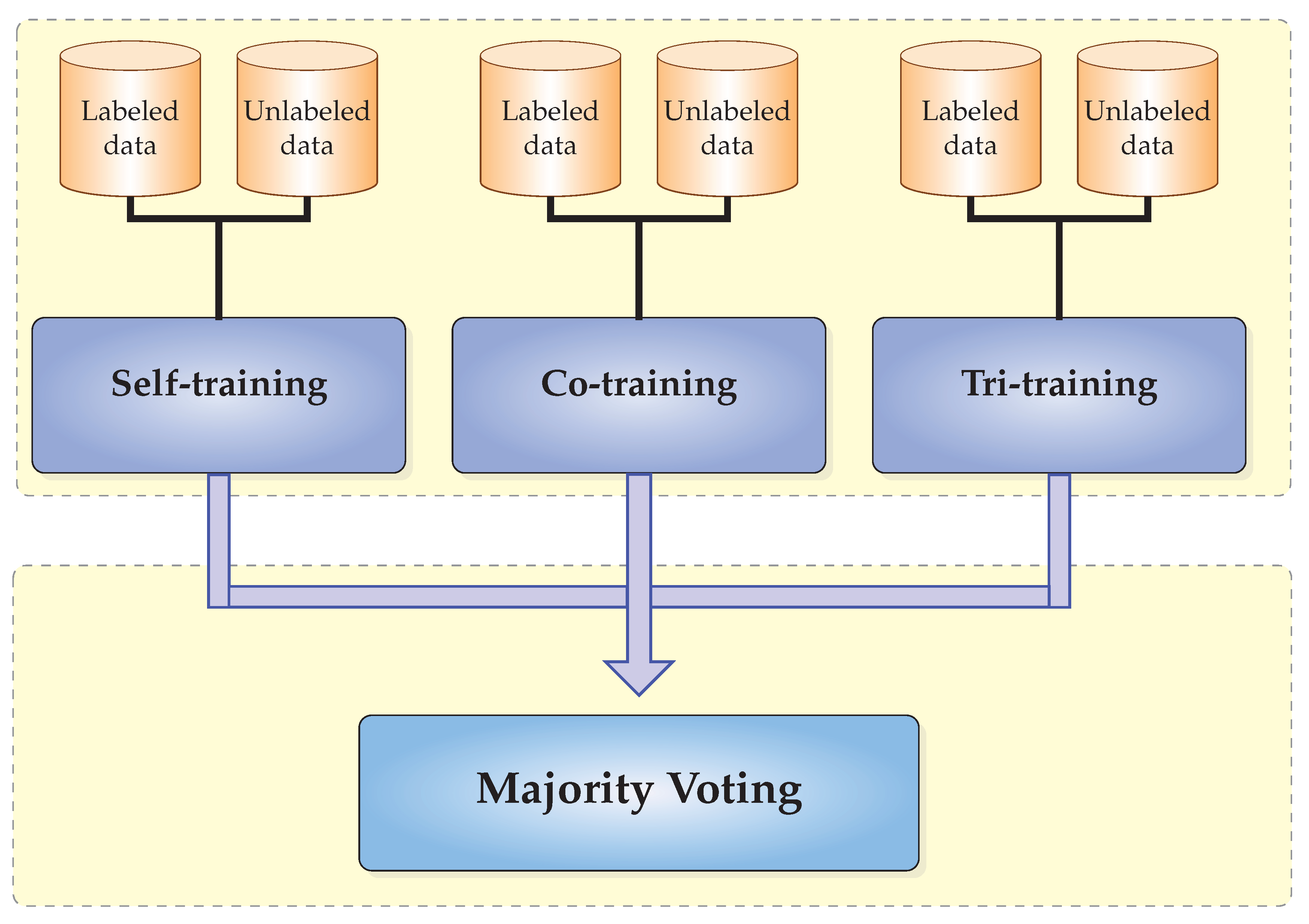
The main and crucial difference between these three learning algorithms is the mechanism used to label unlabeled data. More to the point, self-training and tri-training are single-view methods, while co-training is a multi-view method. Furthermore, it is worth mentioning that co-training and tri-training are indeed ensemble methods, since they both make use of multiple classifiers. An overview of CST-Voting is depicted in Figure 1.

Initially, the classical semi-supervised algorithms, which constitute the ensemble, i.e., self-training, co-training and tri-training, are trained utilizing the same labeled L and unlabeled dataset U. Subsequently, the final hypothesis on an unlabeled example of the test set combines the individual predictions of the SSL algorithms, thus utilizing a simple majority voting methodology. Therefore, the ensemble output is the one made by more than half of them. A high-level description of the proposed CST-Voting is presented in Algorithm 4.    

Algorithm 4: CST-Voting

Input:   L-Set of labeled instances.      U-Set of unlabeled instances.      C-Base learner. Output: The labels of instances in the testing set.   /* Training phase */ 1: Self-training$(L,U)$ 2: Co-training$(L,U)$ 3: Tri-training$(L,U)$   /* Voting phase */ 4: for each $x\in T$ do 5: Apply self-training, co-training and tri-training on x. 6: Use majority vote to predict the label $y^{\ast }$ of x. 7: end for

3. Experimental Results

We conducted a series of experiments in order to evaluate the performance of CST-Voting algorithm compared to the most popular and frequently-used SSL algorithms, which are self-training, co-training and tri-training. All SSL algorithms were evaluated using the following Shenzhen lung mask dataset.

3.1. Dataset Description

The dataset utilized in our work was constructed by manually-segmented lung masks for the Shenzhen Hospital X-ray set as presented in [27]. These segmented lung masks were original utilized for the description of the lung segmentation technique in combination with lossless and lossy data augmentation.

The segmentation masks for the Shenzhen Hospital X-ray set were manually prepared by students and teachers of the Computer Engineering Department, Faculty of Informatics and Computer Engineering, National Technical University of Ukraine “Igor Sikorsky Kyiv Polytechnic Institute” [27]. The set contained 279 normal CXRs and 287 abnormal ones with tuberculosis.

The original Shenzhen Hospital X-ray set contained images from Shenzhen Hospital, which is one of the largest hospitals in China for infectious diseases, with a focus both on their prevention, as well as treatment [7,8]. The X-rays were collected within a one-month period, mostly in September 2012, as a part of the daily routine at Shenzhen Hospital, using a Philips DR Digital Diagnost system.

3.2. Performance Evaluation of SSL Algorithms

All SSL algorithms were evaluated by deploying as base learners the Naive Bayes (NB) [28], Multilayer Perceptron (MLP) [29], Sequential Minimum Optimization (SMO) [30], the 3NN algorithm [31] RIPPER(JRip) [32] as a rule-learning algorithm and the $C4.5$ decision tree algorithm [33]. These algorithms are some of the most popular machine learning algorithms for classification problems [34].

The implementation code was written in Java, using the WEKA Machine Learning Toolkit [35], and the classification accuracy was evaluated using the stratified 10-fold cross-validation. In this validation, the data were separated into folds so that each fold had the same distribution of grades as the entire dataset. Similar to Blum and Mitchell [11], a limit to the number of iterations of all SSL algorithms was established. The proposed implementation strategy had also been adopted by many researchers as stated in [12,15,16,17,21,36]. In order to study the influence of the amount of labeled data, three different ratios (R) of the training data were used, i.e., $10\%$, $20\%$ and $30\%$.

The configuration parameters for all SSL algorithms, utilized in our experiments, are presented in

Table 1. Parameter specification for all the Semi-Supervised Learning (SSL) methods employed in our experiments.

SSL Algorithm	Parameters
Self-training	$\mathrm{MaxIter}=40$.
	$ConLev=95\%$.
Co-training	$\mathrm{MaxIter}=40$.
	$\mathrm{Initial}\mathrm{unlabeled}\mathrm{pool}=75$.
Tri-training	No parameters specified.

. Furthermore, in order to minimize the effect of any expert bias, instead of attempting to tune any of the algorithms to the specific datasets, all base learners were used with their default parameter settings included in the Weka library [37].

To evaluate the performance of the SSL classification algorithms, the following three performance metrics are considered, namely Sensitivity (Sen), Specificity (Spe) and Accuracy (Acc):

$$\begin{array}{ccc}\hfill Sen& =& {\displaystyle \frac{TP}{TP+FN}}\hfill \\ \hfill Spe& =& {\displaystyle \frac{TN}{TN+FP}}\hfill \\ \hfill Acc& =& {\displaystyle \frac{TP+TN}{TP+TN+FP+FN}}\hfill \end{array}$$

where $TP$ stands for the number of normal patients who are identified as normal, $TN$ for the number of abnormal patients who are identified as abnormal, $FP$ (type I error) for the number of normal patients who are identified as abnormal and $FN$ (type II error) for the number of abnormal patients who are identified as normal.

The sensitivity of classification was the proportion of actual positives that were predicted as positive; in the following, specificity represents the proportion of actual negatives that were predicted as negative, while accuracy was the ratio of correct predictions of a classification model.

Additionally, since it is crucial for a prediction model to accurately identify abnormal patients, the following performance metric was considered:

$$F_{1.5}=\frac{(1+{1.5}^2)TP}{(1+{1.5}^2)TP+{1.5}^{2}FN+FP}$$

which constitutes a harmonic mean of precision. In particular, this metric takes into account the accuracy for both normal and abnormal patients and poses additional weight for abnormal patients instead of for normal ones [38]. Obviously, from a medical perspective, it is better to misidentify an “abnormal” patient than a “normal” one.

Table 2. Accuracy of the SSL algorithms based on the $Sen$ performance metric for each labeled ratio.

			$\mathit{R}=10\%$						$\mathit{R}=20\%$						$\mathit{R}=30\%$
			Self	Co	Tri	CST			Self	Co	Tri	CST			Self	Co	Tri	CST
NB			65.9%	64.2%	67.0%	66.7%			68.1%	67.4%	66.7%	67.4%			68.8%	69.5%	69.5%	69.5%
MLP			68.5%	68.5%	70.3%	69.9%			69.2%	68.5%	65.9%	69.9%			71.7%	69.9%	69.9%	72.4%
SMO			66.7%	66.3%	68.5%	69.9%			67.7%	66.3%	69.9%	73.8%			67.4%	67.0%	68.8%	70.3%
3NN			68.8%	58.1%	65.2%	65.9%			67.7%	65.2%	64.9%	66.3%			66.3%	68.8%	65.9%	68.5%
JRip			67.0%	66.3%	70.6%	69.5%			70.6%	65.6%	69.9%	70.3%			70.6%	69.5%	70.3%	70.6%
C4.5			63.1%	71.0%	64.2%	66.3%			67.7%	70.6%	67.4%	69.5%			62.0%	69.9%	64.5%	67.0%

,

Table 3. Accuracy of the SSL algorithms based on the $Spe$ performance metric for each labeled ratio.

			$\mathit{R}=10\%$						$\mathit{R}=20\%$						$\mathit{R}=30\%$
			Self	Co	Tri	CST			Self	Co	Tri	CST			Self	Co	Tri	CST
NB			65.5%	65.9%	65.2%	66.2%			65.2%	65.9%	66.9%	65.9%			66.6%	65.9%	66.6%	67.2%
MLP			66.6%	67.2%	65.5%	64.8%			66.2%	66.6%	71.1%	69.3%			66.2%	68.3%	66.9%	69.3%
SMO			64.5%	69.3%	69.3%	69.0%			64.8%	70.0%	62.4%	66.6%			65.2%	70.0%	69.0%	69.0%
3NN			62.4%	67.9%	66.2%	66.9%			63.8%	67.6%	63.1%	67.6%			68.6%	65.2%	66.6%	68.6%
JRip			66.2%	61.7%	67.9%	68.6%			66.2%	64.8%	66.9%	69.0%			68.6%	65.9%	68.6%	69.0%
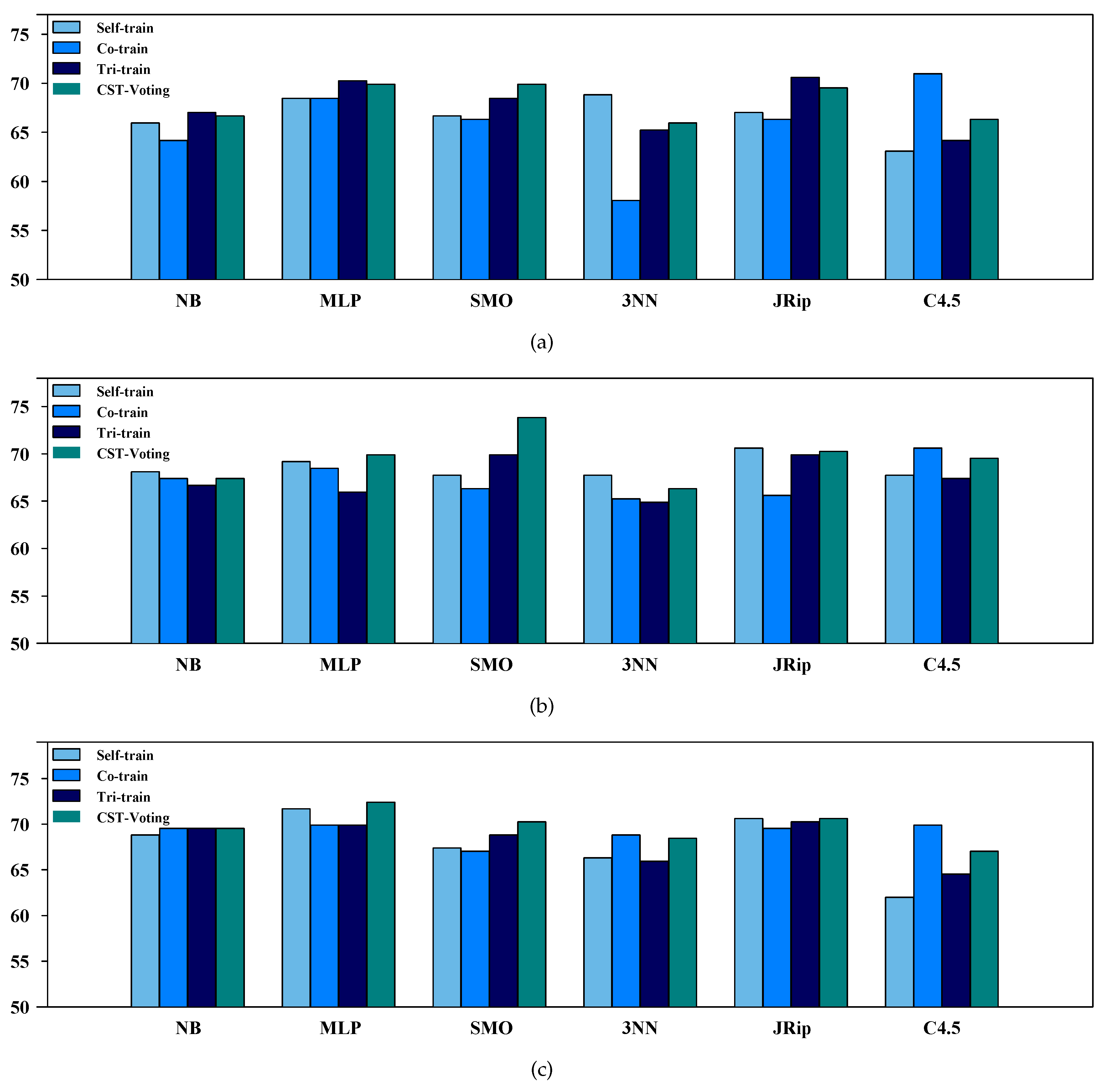
C4.5			69.7%	54.0%	70.0%	68.3%			67.2%	58.5%	66.6%	66.6%			68.6%	65.9%	69.3%	69.3%

and

Table 4. Accuracy of the SSL algorithms based on the $F_{1.5}$ performance metric for each labeled ratio.

			$\mathit{R}=10\%$						$\mathit{R}=20\%$						$\mathit{R}=30\%$
			Self	Co	Tri	CST			Self	Co	Tri	CST			Self	Co	Tri	CST
NB			65.8%	65.7%	65.7%	66.5%			65.9%	66.4%	67.0%	66.4%			67.2%	66.8%	67.3%	67.9%
MLP			67.1%	67.7%	66.6%	66.0%			67.0%	67.1%	70.2%	69.6%			67.5%	68.8%	67.7%	70.2%
SMO			65.1%	68.9%	69.3%	69.4%			65.6%	69.4%	64.0%	68.2%			65.8%	69.6%	69.1%	69.4%
3NN			63.8%	66.2%	66.2%	66.9%			64.7%	67.3%	63.6%	67.5%			68.3%	66.1%	66.6%	68.8%
JRip			66.6%	62.7%	68.7%	69.0%			67.3%	65.2%	67.7%	69.4%			69.2%	66.8%	69.2%	69.5%
C4.5			68.5%	57.1%	69.0%	68.1%			67.5%	61.0%	66.9%	67.3%			67.5%	66.9%	68.5%	69.0%

present the accuracy of each SSL algorithm based on the performance metrics $Sen$, $Spe$ and $F_{1.5}$, respectively. Notice that the highest classification accuracy is underlined. Firstly, it is worth mentioning that CST-Voting performed better in five out of six cases for a $30\%$ labeled ratio for each performance metric and improved its classification accuracy as the labeled ratio increased.

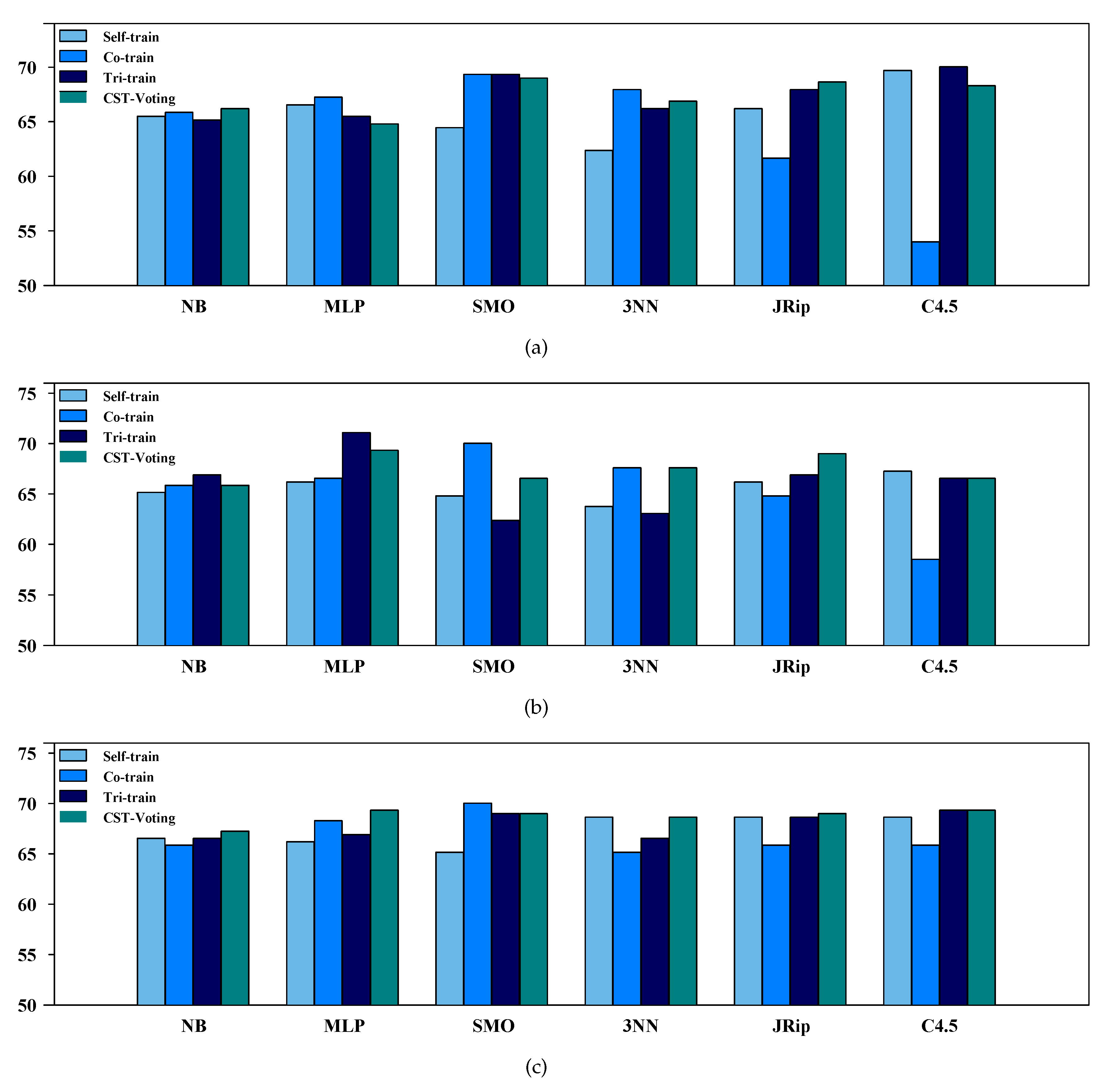
Moreover, relative to the performance metrics $Sen$ and $Spe$, the proposed algorithm exhibited the best or the second best accuracy, independent of the classifier utilized as the base learner and the value of the labeled ratio. Regarding the $F_{1.5}$ metric, CST-Voting exhibited the highest accuracy reporting the top performance in 4, 2 and 5 cases for a $10\%$, $20\%$ and $30\%$ labeled ratio, respectively, while self-training achieved the worst performance. Finally, a more representative visualization of the accuracy of the compared SSL is presented in Figure 2, Figure 3 and Figure 4. Each box-plot presents the accuracy measure for each tested SSL algorithm according to the supervised base learner and labeled ratio.

Table 5. Performance evaluation of the SSL algorithm relative to the performance metric $Acc$ for each labeled ratio.

			$\mathit{R}=10\%$						$\mathit{R}=20\%$						$\mathit{R}=30\%$
			Self	Co	Tri	CST			Self	Co	Tri	CST			Self	Co	Tri	CST
NB			65.7%	65.0%	66.1%	66.4%			66.6%	66.6%	66.8%	66.6%			67.6%	67.8%	68.0%	68.4%
MLP			67.5%	67.5%	67.8%	67.3%			67.6%	67.8%	68.5%	69.6%			68.9%	69.1%	68.4%	70.8%
SMO			65.5%	67.8%	68.9%	69.4%			66.2%	68.2%	68.0%	68.2%			66.2%	68.6%	68.9%	69.6%
3NN			65.6%	63.1%	65.7%	66.5%			65.7%	66.4%	64.0%	67.0%			67.5%	66.9%	66.3%	68.6%
JRip			66.6%	64.0%	69.2%	69.1%			68.4%	65.2%	68.4%	69.6%			69.6%	67.7%	69.4%	69.8%
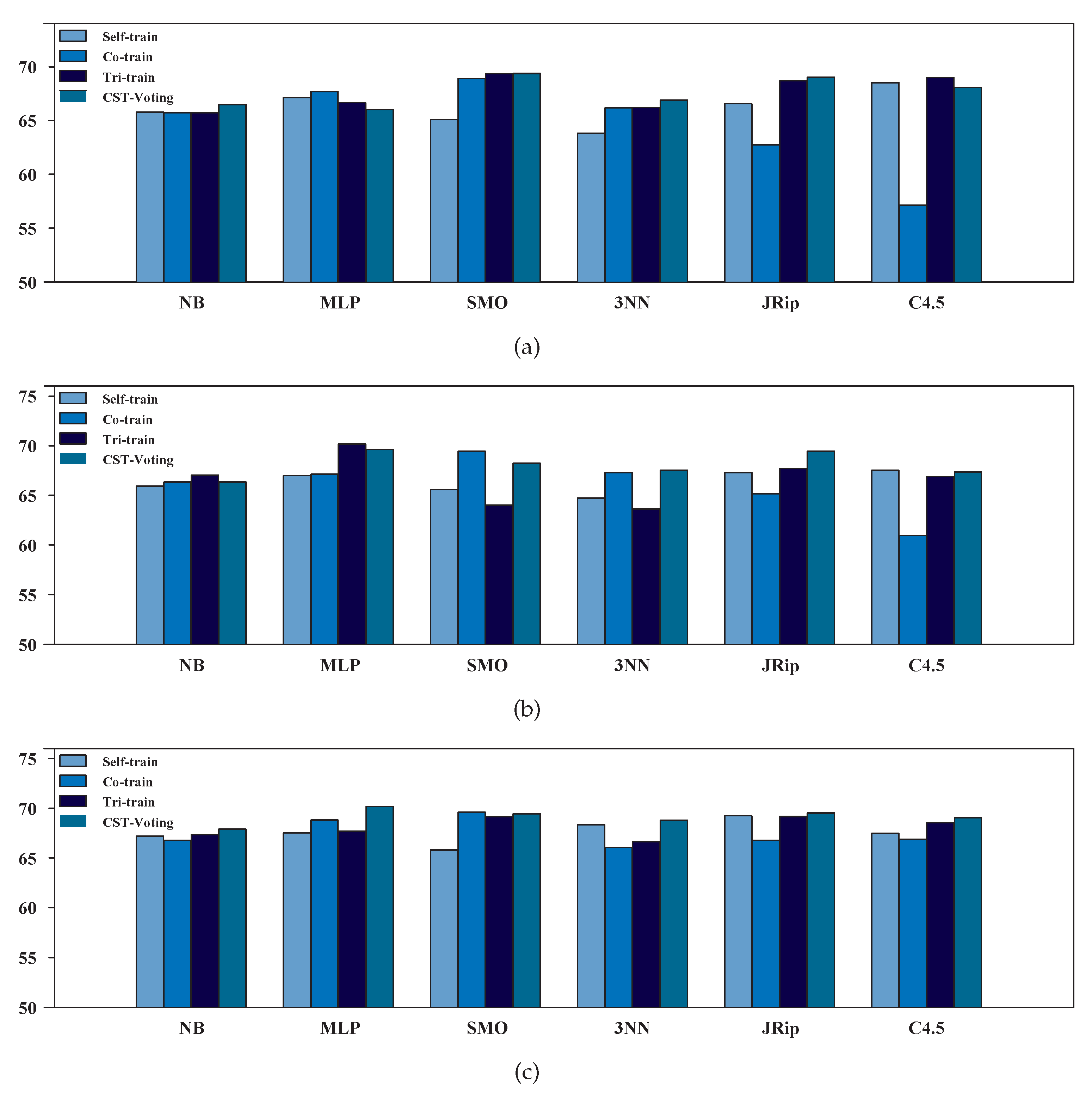
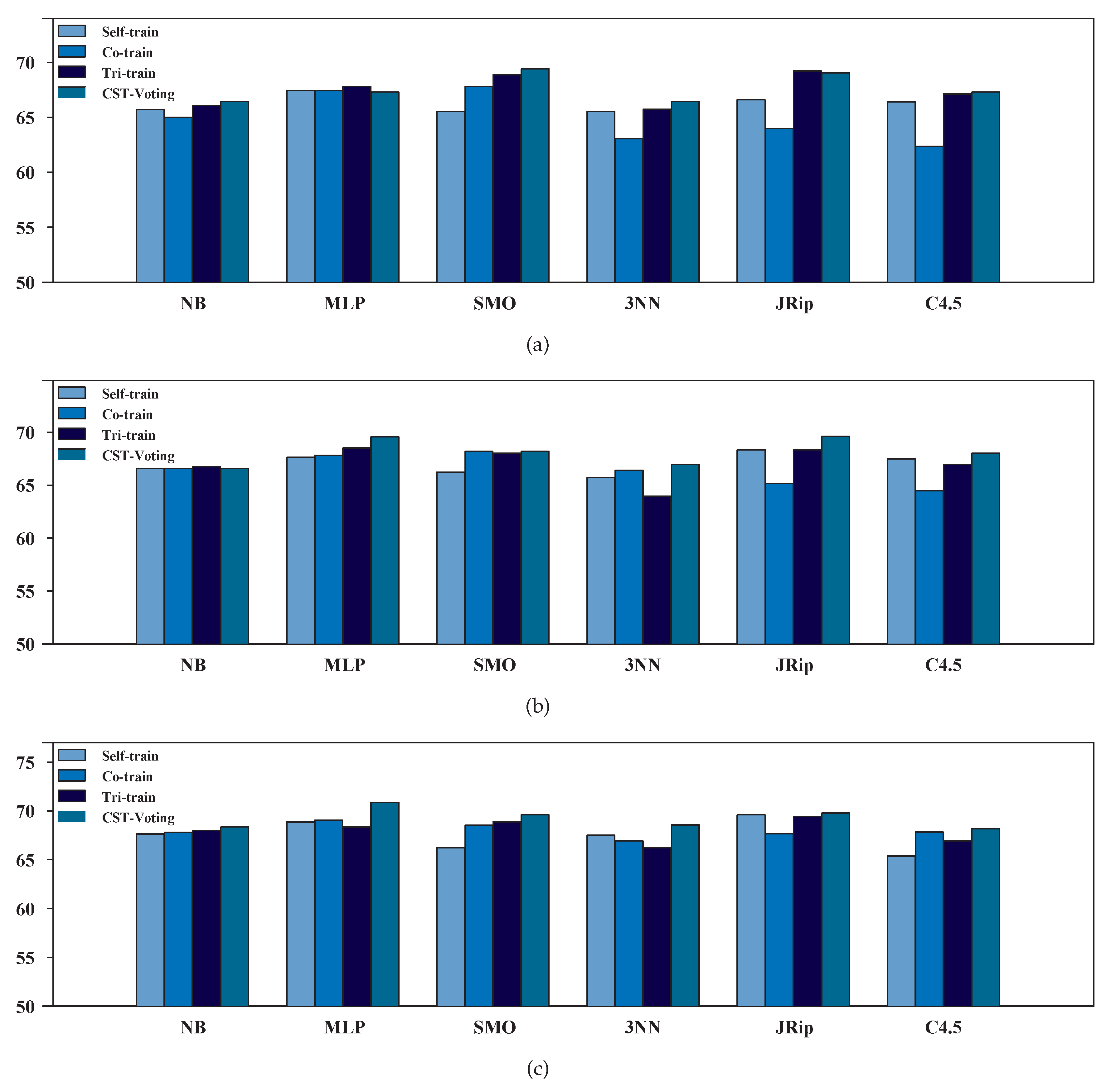
C4.5			66.4%	62.4%	67.1%	67.3%			67.5%	64.5%	67.0%	68.0%			65.4%	67.8%	67.0%	68.2%

presents the classification accuracy of all SSL algorithms based on the performance metric $Acc$, regarding each labeled ratio. As mentioned above, the accuracy measure of the best-performing SSL algorithm is underlined for each base learner. The aggregated results showed that CST-Voting was by far the most efficient and robust method independent of the utilized ratio of labeled instances in the training set. In more detail, CST-Voting performed better in four out of six cases for a $10\%$ labeled ratio and in all cases for a $20\%$ and $30\%$ labeled ratio. Furthermore, a more representative visualization of the classification accuracy of all compared SSL algorithms is presented in Figure 5. Finally, it is worth mentioning that CST-Voting achieved a much better classification performance as the labeled ratio increased.

3.3. Statistical and Post-Hoc Analysis

In machine learning, the statistical comparison of multiple algorithms over multiple datasets is fundamental, and it is usually carried out by means of a statistical test [16]. Since our motivation stems from the fact that we are interested in evaluating the rejection of the hypothesis that all the algorithms perform equally well for a given level based on their classification accuracy and highlighting the existence of significant differences between our proposed algorithm and the classical SSL algorithms, we utilized the non-parametric Friedman Aligned Ranking (FAR) [39] test.

Let $r_i^j$ be the rank of the j-th of k learning algorithms on the i-th of N problems. Under the null-hypothesis $H_0$, which states that all the algorithms are equivalent, the Friedman aligned ranks test statistic is defined by:

$$F_{AR}=\frac{(k-1)\left[{\displaystyle \sum _{j=1}^k{\widehat{R}}_j^2-(k{N}^2/4){(kN+1)}^2}\right]}{{\displaystyle \frac{kN(kN+1)(2kN+1)}{6}-\frac{1}{k}\sum _{i=1}^N{\widehat{R}}_i^2}}$$

where ${\widehat{R}}_i$ is equal to the rank total of the i-th dataset and ${\widehat{R}}_j$ is the rank total of the j-th algorithm. The test statistic $F_{AR}$ is compared with the ${\chi }^2$ distribution with $(k-1)$ degrees of freedom. Notice that, since the test is non-parametric, it does not require the commensurability of the measures across different datasets. In addition, this test does not assume the normality of the sample means, and thus, it is robust to outliers.

In statistical hypothesis testing, the p-value is the probability of obtaining a result at least as extreme as the one that was actually observed, assuming that the null hypothesis is true. In other words, the p-value provides information about whether a statistical hypothesis test is significant or not, indicating “how significant” the result is while it does this without committing to a particular level of significance. When a p-value is considered in a multiple comparison, it reflects the probability error of a certain comparison; however, it does not take into account the remaining comparisons belonging to the family. One way to address this problem is to report adjusted p-values, which take into account that multiple tests are conducted and can be compared directly with any significance level [40].

To this end, the Finner post-hoc test [41] with a significance level $\alpha =0.05$ was applied to detect the specific differences among the algorithms. More to the point, the Finner test is easy to comprehend, and it usually offers better results than other post-hoc tests, such as the Holm [42] or Hochberg test [43], especially when the number of compared algorithms is low [40].

The Finner procedure adjusts the value of $\alpha$ in a step-down manner. Let $p_1,p_2,\dots ,p_{k-1}$ be the ordered p-values with $p_1\le p_2\le \cdots \le p_{k-1}$ and $H_1,H_2,\dots ,H_{k-1}$ be the corresponding hypothesis. The Finner procedure rejects $H_1$–$H_{i-1}$ if i is the smallest integer such that $p_i>1-{(1-\alpha )}^{(k-1)/i}$, while the adjusted Finner p-value is defined by:

$$p_F=\min \left\{1,max\left\{1-{(1-p_j)}^{(k-1)/j)}\right\}\right\},$$

where $p_j$ is the p-value obtained for the j-th hypothesis and $1\le j\le i$. It is worth mentioning that the test rejects the hypothesis of equality when the $p_F$ is less than $\alpha$.

Table 6. Friedman Aligned Ranking (FAR) test and Finner post-hoc test (labeled ratio 10%).

SSL Algorithm	Friedman Aligned	Finner Post-Hoc Test
	Ranking	${\mathit{p}}_{\mathit{F}}$-value	Null Hypothesis
CST-Voting	6.8333	-	-
Tri-training	8.0000	0.775051	accepted
Self-training	15.3333	0.037336	rejected
Co-training	19.8333	0.001451	rejected

,

Table 7. FAR test and Finner post-hoc test (labeled ratio 20%).

SSL Algorithm	Friedman Aligned	Finner Post-Hoc Test
	Ranking	${\mathit{p}}_{\mathit{F}}$-value	Null Hypothesis
CST-Voting	5.75	-	-
Tri-training	13.50	0.047649	rejected
Self-training	15.00	0.023465	rejected
Co-training	15.75	0.014306	rejected

and

Table 8. FAR test and Finner post-hoc test (labeled ratio 30%).

SSL Algorithm	Friedman Aligned	Finner Post-Hoc Test
	Ranking	${\mathit{p}}_{\mathit{F}}$-value	Null Hypothesis
CST-Voting	4.1667	-	-
Tri-training	14.1667	0.014306	rejected
Co-training	14.5000	0.011369	rejected
Self-training	17.1667	0.001451	rejected

present the information of the statistical analysis performed by nonparametric multiple comparison procedures over $10\%$, $20\%$ and $30\%$ of labeled data, respectively. The best (e.g., lowest) ranking obtained in each FAR test determined the control algorithm for the post-hoc test. Moreover, the adjusted p-value with Finner’s test ($p_F$) was presented based on the control algorithm, at the $\alpha =0.05$ level of significance. Clearly, CST-Voting achieved the best performance due to better probability-based ranking and higher classification accuracy.

4. Conclusions

In this work, we evaluated the performance of an ensemble SSL algorithm for the classification of CXRs of tuberculosis, entitled CST-Voting. CST-Voting combines the individual predictions of three popular SSL algorithms, i.e., co-training, self-training and tri-training, utilizing a simple voting methodology. A plethora of experiments were carried out illustrating the effectiveness of the proposed algorithm, as statistically confirmed by the Friedman aligned ranks nonparametric test, as well as the Finner post-hoc test. The dataset utilized was constituted by manually-segmented lung masks for X-ray sets, which were originally utilized for the description of a novel lung segmentation technique.

Our future work is concentrated on expanding our experiments and on further applying the proposed algorithm to several biomedical datasets for image classification. Furthermore, another interesting aspect is the development of a parallel implementation of our proposed algorithm. Notice that the implementation of each component-based learner in parallel machines constitutes a significant aspect to be studied, since a huge amount of data can be processed in significantly less computational time.

References

- Livieris, I.E.; Apostolopoulou, M.S.; Sotiropoulos, D.G.; Sioutas, S.A.; Pintelas, P. Classification of large biomedical data using ANNs based on BFGS method. In Proceedings of the 13th Panhellenic Conference on Informatics (PCI’19), Corfu, Greece, 10–12 September 2009; pp. 87–91. [Google Scholar]
- Melendez, J.; van Ginneken, B.; Maduskar, P.; Philipsen, R.; Reither, K.; Breuninger, M.; Adetifa, I.; Maane, R.; Ayles, H.; Sánchez, C. A novel multiple-instance learning-based approach to computer-aided detection of tuberculosis on chest X-rays. IEEE Trans. Med. Imaging 2015, 34, 179–192. [Google Scholar] [CrossRef] [PubMed]
- Doi, K. Computer-aided diagnosis in medical imaging: historical review, current status and future potential. Comput. Med. Imaging Graph. 2007, 31, 198–211. [Google Scholar] [CrossRef] [PubMed]
- Rangayyan, R.; Suri, J. Recent Advances in Breast Imaging, Mammography, and Computer-Aided Diagnosis of Breast Cancer; SPIE Publications: Bellingham, WA, USA, 2006. [Google Scholar]
- Hogeweg, L.; Mol, C.; de Jong, P.; Ayles, R.; van Ginneken, B. Fusion of local and global detection systems to detect tuberculosis in chest radiographs. Med. Image Comput. Comput.-Assist. Interv. 2010, 13, 650–657. [Google Scholar] [PubMed]
- Hogeweg, L.; Sánchez, C.; de Jong, P.; Maduskar, P.; van Ginneken, B. Clavicle segmentation in chest radiographs. Med. Image Anal. 2012, 16, 1490–1502. [Google Scholar] [CrossRef] [PubMed]
- Jaeger, S.; Karargyris, A.; Candemir, S.; Folio, L.; Siegelman, J.; Callaghan, F.; Xue, Z.; Palaniappan, K.; Singh, R.; Antani, S.; et al. Automatic tuberculosis screening using chest radiographs. IEEE Trans. Med. Imaging 2014, 33, 233–245. [Google Scholar] [CrossRef] [PubMed]
- Candemir, S.; Jaeger, S.; Musco, K.P.J.; Singh, R.; Xue, Z.; Karargyris, A.; Antani, S.; Thoma, G.; McDonald, C. Lung segmentation in chest radiographs using anatomical atlases with nonrigid registration. IEEE Trans. Med. Imaging 2014, 33, 577–590. [Google Scholar] [CrossRef] [PubMed]
- Zhu, X.; Goldberg, A. Introduction to semi-supervised learning. Synth. Lect. Artif. Intell. Mach. Learn. 2009, 3, 1–130. [Google Scholar] [CrossRef]
- Blum, A.; Chawla, S. Learning from labeled and unlabeled data using graph mincuts. In Proceedings of the 8th International Conference on Machine Learning (ICML), Williamstown, MA, USA, 28 June–1 July 2001; pp. 19–26. [Google Scholar]
- Blum, A.; Mitchell, T. Combining labeled and unlabeled data with co-training. In Proceedings of the 11th Annual Conference on Computational Learning Theory, Madison, WI, USA, 24–26 July 1998; pp. 92–100. [Google Scholar]
- Triguero, I.; García, S.; Herrera, F. Self-labeled techniques for semi-supervised learning: Taxonomy, software and empirical study. Knowl. Inform. Syst. 2015, 42, 245–284. [Google Scholar] [CrossRef]
- Nigam, K.; Ghani, R. Analyzing the effectiveness and applicability of co-training. In Proceedings of the ACM International Conference on Information and Knowledge Management, McLean, VA, USA, 6–11 November 2000; pp. 86–93. [Google Scholar]
- Guo, T.; Li, G. Improved tri-training with unlabeled data. In Software Engineering and Knowledge Engineering: Theory and Practice; Springer: Berlin, Heidelberg/ Germany, 2012; pp. 139–147. [Google Scholar]
- Liu, C.; Yuen, P. A boosted co-training algorithm for human action recognition. IEEE Trans. Circuits Syst. Video Technol. 2011, 21, 1203–1213. [Google Scholar] [CrossRef]
- Livieris, I.; Drakopoulou, K.; Tampakas, V.; Mikropoulos, T.; Pintelas, P. Predicting secondary school students’ performance utilizing a semi-supervised learning approach. J. Educ. Comput. Res. 2018. [Google Scholar] [CrossRef]
- Livieris, I.; Drakopoulou, K.; Tampakas, V.; Mikropoulos, T.; Pintelas, P. An ensemble-based semi-supervised approach for predicting students’ performance. In Research on e-Learning and ICT in Education; Elsevier: New York, NY, USA, 2018. [Google Scholar]
- Zhou, Z.; Li, M. Tri-training: Exploiting unlabeled data using three classifiers. IEEE Trans. Knowl. Data Eng. 2005, 17, 1529–1541. [Google Scholar] [CrossRef]
- Zhu, X. Semi-supervised learning. In Encyclopedia of Machine Learning; Springer: New York, NY, USA, 2011; pp. 892–897. [Google Scholar]
- Sigdel, M.; Dinç, I.; Dinç, S.; Sigdel, M.; Pusey, M.; Aygün, R. Evaluation of semi-supervised learning for classification of protein crystallization imagery. In Proceedings of the IEEE Southeastcon 2014, Lexington, KY, USA, 13–16 March 2014; pp. 1–6. [Google Scholar]
- Triguero, I.; Sáez, J.; Luengo, J.; García, S.; Herrera, F. On the characterization of noise filters for self-training semi-supervised in nearest neighbor classification. Neurocomputing 2014, 132, 30–41. [Google Scholar] [CrossRef]
- Ng, V.; Cardie, C. Weakly supervised natural language learning without redundant views. In Proceedings of the 2003 conference of the North American Chapter of the Association for Computational Linguistics on Human Language Technology, Edmonton, AB, Canada, 27 May–1 June 2003; Volume 1, pp. 94–101. [Google Scholar]
- Roli, F.; Marcialis, G. Semi-supervised PCA-based face recognition using self-training. Joint IAPR International Workshops on Statistical Techniques in Pattern Recognition (SPR) and Structural and Syntactic Pattern Recognition (SSPR); Springer: Berlin/Heidelberg, Germany, 2006; pp. 560–568. [Google Scholar]
- Sun, S.; Jin, F. Robust co-training. Int. J. Pattern Recognit. Artif. Intell. 2011, 25, 1113–1126. [Google Scholar] [CrossRef]
- Du, J.; Ling, C.; Zhou, Z. When does co-training work in real data? IEEE Trans. Knowl. Data Eng. 2011, 23, 788–799. [Google Scholar] [CrossRef]
- Kostopoulos, G.; Livieris, I.E.; Kotsiantis, S.; Tampakas, V. CST-Voting-A semi-supervised ensemble method for classification problems. J. Intell. Fuzzy Syst. 2018, 1–11. [Google Scholar] [CrossRef]
- Stirenko, S.; Kochura, Y.; Alienin, O.; Rokovyi, O.; Gang, P.; Zeng, W.; Gordienko, Y. Chest X-ray analysis of tuberculosis by deep learning with segmentation and augmentation. arXiv, 2018; arXiv:1803.01199. [Google Scholar]
- Domingos, P.; Pazzani, M. On the optimality of the simple Bayesian classifier under zero-one loss. Mach. Learn. 1997, 29, 103–130. [Google Scholar] [CrossRef]
- Rumelhart, D.; Hinton, G.; Williams, R. Learning internal representations by error propagation. In Parallel Distributed Processing: Explorations in The Microstructure of Cognition; Rumelhart, D., McClelland, J., Eds.; MIT Press: Cambridge, MA, USA, 1986; pp. 318–362. [Google Scholar]
- Platt, J. Using sparseness and analytic QP to speed training of support vector machines. In Advances in Neural Information Processing Systems; Kearns, M., Solla, S., Cohn, D., Eds.; MIT Press: Cambridge, MA, USA, 1999; pp. 557–563. [Google Scholar]
- Aha, D. Lazy Learning; Kluwer Academic Publishers: Dordrecht, The Netherlands, 1997. [Google Scholar]
- Cohen, W. Fast effective rule induction. In Proceedings of the International Conference on Machine Learning, Tahoe City, CA, USA, 9–12 July 1995; pp. 115–123. [Google Scholar]
- Quinlan, J. C4.5: Programs for Machine Learning; Morgan Kaufmann: San Francisco, CA, USA, 1993. [Google Scholar]
- Wu, X.; Kumar, V.; Quinlan, J.; Ghosh, J.; Yang, Q.; Motoda, H.; McLachlan, G.; Ng, A.; Liu, B.; Yu, P.; et al. Top 10 algorithms in data mining. Knowl. Inf. Syst. 2008, 14, 1–37. [Google Scholar] [CrossRef]
- Hall, M.; Frank, E.; Holmes, G.; Pfahringer, B.; Reutemann, P.; Witten, I. The WEKA data mining software: An update. SIGKDD Explor. Newslett. 2009, 11, 10–18. [Google Scholar] [CrossRef]
- Tanha, J.; van Someren, M.; Afsarmanesh, H. Semi-supervised self-training for decision tree classifiers. Int. J. Mach. Learn. Cybern. 2015, 8, 355–370. [Google Scholar] [CrossRef] [Green Version]
- Weka 3: Data Mining Software in Java. Available online: https://www.cs.waikato.ac.nz/ml/weka/ (accessed on 15 July 2018).
- Van Rijsbergen, C. Information Retrieval, 2nd ed.; Butterworths: London, UK, 1979. [Google Scholar]
- Hodges, J.; Lehmann, E. Rank methods for combination of independent experiments in analysis of variance. Ann. Math. Stat. 1962, 33, 482–497. [Google Scholar] [CrossRef]
- García, S.; Fernández, A.; Luengo, J.; Herrera, F. Advanced nonparametric tests for multiple comparisons in the design of experiments in computational intelligence and data mining: Experimental analysis of power. Inf. Sci. 2010, 180, 2044–2064. [Google Scholar] [CrossRef]
- Finner, H. On a monotonicity problem in step-down multiple test procedures. J. Am. Stat. Assoc. 1993, 88, 920–923. [Google Scholar] [CrossRef]
- Holm, S. A simple sequentially rejective multiple test procedure. Scandi. J. Stat. 1979, 6, 65–70. [Google Scholar]
- Hochberg, Y. A sharper Bonferroni procedure for multiple tests of significance. Biometrika 1988, 75, 800–802. [Google Scholar] [CrossRef]
Figure 1.
CST-Voting.
Figure 2.
Box plot for performance metric for each labeled ratio. (a) Ratio = 10%; (b) ratio = 20%; (c) ratio = 30%.
Figure 3.
Box plot for the performance metric for each labeled ratio. (a) Ratio = 10%; (b) ratio = 20%; (c) ratio = 30%.
Figure 4.
Figure 5.