
What Features of Ligands Are Relevant to the Opening of Cryptic Pockets in Drug Targets?


1
Institute of Structural Biology, Molecular Targets and Therapeutics Center, Helmholtz Munich-Deutsches Forschungszentrum für Gesundheit und Umwelt (GmbH), D-85764 Neuherberg, Germany
2
Department of Chemistry, Bayerisches NMR-Zentrum, Technical University of Munich, D-85747 Garching, Germany
3
BIGCHEM GmbH, D-85716 Unterschleißheim, Germany
*
Author to whom correspondence should be addressed.
Informatics 2022, 9(1), 8; https://doi.org/10.3390/informatics9010008
Submission received: 25 November 2021
/
Revised: 19 January 2022
/
Accepted: 20 January 2022
/
Published: 25 January 2022
(This article belongs to the Special Issue Exclusive Papers Collection of Editorial Board Members and Scholars Invited by Editorial Board Members of Informatics)
Abstract
:Small-molecule drug design aims to identify inhibitors that can specifically bind to a functionally important region on the target, i.e., an active site of an enzyme. Identification of potential binding pockets is typically based on static three-dimensional structures. However, small molecules may induce and select a dynamic binding pocket that is not visible in the apo protein, which presents a well-recognized challenge for structure-based drug discovery. Here, we assessed whether it is possible to identify features in molecules, which we refer to as inducers, that can induce the opening of cryptic pockets. The volume change between apo and bound protein conformations was used as a metric to differentiate chemical features in inducers vs. non-inducers. Based on the dataset of holo–apo pairs, classification models were built to determine an optimum threshold. The model analysis suggested that inducers preferred to be more hydrophobic and aromatic. The impact of sulfur was ambiguous, while phosphorus and halogen atoms were overrepresented in inducers. The fragment analysis showed that small changes in the structures of molecules can strongly affect the potential to induce a cryptic pocket. This analysis and developed model can be used to design inducers that can potentially open cryptic pockets for undruggable proteins.
1. Introduction
Receptor-based drug design is performed when a new drug target is discovered and the protein structure is available to be explored. Provided that it has (a) druggable pocket(s), virtual screening of a chemical library, such as by docking a large number of compounds into the binding pocket and selecting promising compounds followed by their biological testing, is one of the most efficient ways to find active compounds. However, sometimes, the determined pockets are not druggable, which means that their targeting does not cause sufficient inhibition, activation, or selectivity as is required for a proper biological response [1]. Structure-based drug discovery usually focuses on small-molecule therapeutic agents. Two decades ago, Hopkins and Groom estimated that only ~10–14% of the human proteome was druggable [2]. Further, they identified only 120 out of ~600–1500 potential drug targets as targets of approved small-molecule drugs. By 2017, the number of targets for small-molecule drugs plus biologic drugs had reached 601 [3,4].
For the remaining 85% of “undruggable” proteins, one can explore their conformational changes, which contribute to the appearance of new pockets, to make them druggable. Imatinib (Figure 1) is an antineoplastic agent, which inhibits the Abelson (Abl) tyrosine kinase by capturing a transient state [5,6,7,8]. It specifically binds with the preformed ATP pocket and an adjacent allosteric pocket, which likely appears after being induced by the ligand itself. Both experimental and computational approaches were used to explore the existence of transient pockets, also known as cryptic sites [9]. Cryptic binding sites are absent or occluded in unbound proteins but are present in ligand-bound structures. Mizukoshi et al. developed a strategy to identify cryptic sites and manipulate their dynamic changes through nuclear magnetic resonance (NMR) combined with allosteric mutations [10]. Kii et al. identified an inhibitor (FINDY) targeting transient pockets in dual-specificity tyrosine-phosphorylation-regulated kinase 1A (DYRK1A), although the folding intermediate interfered with by FINDY has not been determined [11]. Cimermancic et al. created the CryptoSite dataset of apo–holo pairs with cryptic sites and used machine learning to predict cryptic sites with relatively high accuracy (AUC = 0.83) [12]. They found that cryptic sites were less hydrophobic and more flexible than traditional binding pockets. Beglov et al. explored the extended CryptoSite dataset by detecting hot spots using FTMap [13,14]. Their results showed that regions around cryptic sites had above-average flexibility. Moreover, they observed that cryptic sites, which were formed solely by side-chain motion or the motion of less than five backbone residues, showed weak ligand binding potential with limited use for drug discovery. Clark et al. investigated the structural flexibility of proteins by root-mean-square deviation (RMSD) calculations of backbone atoms and Χ1 angles of side-chain atoms [15]. The ligand-induced backbone flexibility across apo–holo pairs was slightly larger than the inherent backbone flexibility of the apo and holo states. Upon ligand binding, side-chain Χ1 angles were frequently pushed into new orientations outside the range seen in apo states. They found that the influences on binding site variation could not be easily attributed to features such as ligand size or X-ray structure resolution. More recently, Evans et al. developed a machine learning method (TACTICS) to predict cryptic sites [16]. TACTICS was trained on an extended CryptoSite dataset and used molecular dynamics (MD) simulation data as input. This advanced method successfully detected the active sites and multiple allosteric sites in the SARS-CoV-2 main protease. The increasing use of MD simulations in conjunction with machine learning algorithms will likely contribute immensely to the identification of cryptic pockets and the expansion of the scale of druggable proteins in the foreseeable future [17].
The aforementioned works studied the cryptic pockets regarding the inherent flexibility and diverse dynamics of the protein. In addition, the ligand contributes to inducing the pocket adjustment to accommodate itself in the binding process as well. We were interested in identifying the structural features of ligands that were important for inducing the opening of cryptic sites. This information can be useful for designing new active compounds targeting currently undruggable proteins or discovering new pockets for underexplored proteins. An inducer fragment library can be screened in a fragment-based approach. To our knowledge, no such study has been reported thus far.
Here, we classified the ligands into two groups: the first group consisted of the ligands that induced the opening of cryptic pockets, called “inducers”, and the second group included those that could not open the pockets, referred to as “non-inducers”. The classification criterion was based on the volume change of the pocket between the unbound state (apo) and the bound state (holo). The degree of enlargement of a pocket considered to be “opening” is discussed.
2. Materials and Methods
2.1. Datasets
2.1.1. Dataset I: PDBbind-CN
PDBbind-CN [18,19] v.2020 includes all types of biomolecular complexes and their experimentally measured binding affinity data deposited in the Protein Data Bank (PDB) [20]. Starting from 5316 crystal structures of holo proteins, we established a dataset comprising apo (does not contain a bound ligand) and holo (complex with a ligand) protein pairs. The protein and ligand structures of the holo complexes were retrieved using their PDB IDs. The requirements were that only one ligand was in the same pocket, as identified by the ligand ID [21], and that the resolution of the crystal structure was better than 2.5 Å. The initial set of apo structures included PDB proteins with the same resolution requirements. The binding pocket was defined by the residues within 10 Å of the cognate ligand. Since we were only interested in drug-like small molecules, holo structures whose identified ligands were peptide-like, cofactors, detergents, or crystal additives were excluded, as suggested in previous work [15]. Next, the sequence of each holo protein was analyzed using the blastp program [22] to generate a list of PDB IDs with descending similarity between the holo and apo protein sequences. We determined that no ligands were bound in the same binding pockets of the apo structure, and the protein pair with the highest similarity score was retained for analysis. Both the retrieval and calculation processes were automatically carried out by the PyMOL [23], blastp, and SiteMap [24,25,26] programs with the help of custom scripts.
Moreover, the CryptoSite dataset [13] was combined with the PDBbind dataset as the training set, which has been commonly used in previous studies on cryptic pockets [9,12,13,16]. Originally, this dataset contained 93 holo proteins, each matching with multiple apo structures. Eight items binding to either multiple ligands or oligosaccharides in the pocket were removed. After the removal of duplicates from the CryptoSite dataset that overlapped with the PDBbind dataset, we retrieved 84 pairs of holo–apo proteins as well as their ligands. All of these ligands were labeled as inducers because the corresponding receptors had cryptic sites that were manually curated and illustrated by the creators.
2.1.2. Dataset II: NR-DBIND
Nuclear receptors (NRs) are important drug targets, and their ligand-binding is generally accompanied by large conformational changes. We implemented the same workflow as the PDBbind dataset to build a dataset comprising apo and holo NR pairs. To this end, the nuclear receptor database (NR-DBIND) [27] was used as the starting point. These data indicated whether the PDB ID corresponded to a holo or apo structure, which helped us to validate the in-house-developed search script.
Below, we describe the tools and procedures used to analyze the retrieved structures and create datasets for analysis.
Structure Preparation and Visualization
PyMOL [23] was used to retrieve structures from the PDB database, define the pocket and align holo–apo pairs. It was also used to visually validate the matching results from in-house scripts.
The quality of starting structures is critical for computational drug design. Therefore, all protein structures were processed using the Schrödinger Protein Preparation Wizard [28]. This script is a tool for correcting common structural problems with experimentally derived structures to create reliable protein models. We used this tool (1) to assign bond orders in known residues and small molecule components based on their SMILES strings in the Chemical Component Dictionary [21], (2) to add explicit hydrogens, and (3) to generate a favorable ligand protonation state based on the number of H-bonds and the Epik penalty score [29].
Identification and Characterization of Binding Pockets
The SiteMap [24,25,26] of the Schrödinger suite was used to identify and calculate the pocket volumes of the preprocessed proteins. This program first detected all sites suitable for docking in the protein structure and then individually calculated the corresponding pocket volume. In this way, we obtained the volumes of the identical pocket in the holo and apo structures. In particular, it was performed using trajectory_binding_site_volumes.py with the -sitemap_site_asl option by specifying the residues constituting the pocket of interest. SiteMap determined the pockets suitable for docking using geometry- and energy-based algorithms. As a result of this restriction, around 1000 input structures failed in this step and thus were not further considered in this work.
The structures that were present in both databases were retained in the PDBbind set for model training and removed from NR-DBIND, which comprised the external validation set. Thus, neither dataset had overlapping structures. In total, we obtained 992 and 135 apo–holo pairs in PDBbind and NR-DBIND, respectively. Among them, 675 and 117 pairs increased the pocket volume, i.e., Vholo − Vapo > 0 Å3. Small changes in the volume could also be due to fluctuations in the volume or restricted conformational adjustments, and thus, the use of a threshold could be beneficial. A detailed procedure for defining the threshold to separate inducers and non-inducers is described in the Results section.
2.2. Methods
2.2.1. Development of Models to Separate Inducers and Non-Inducers
Model Building
We used the OCHEM platform [30] to develop classification models for inducers and non-inducers. The models were developed with data from the PDBbind set, and the NR-DBIND set was used as external validation. We explored different machine learning methods and descriptors available in OCHEM. Random forest (RF) and ALogPS and OEstate (AO) descriptors contributed to the models with the highest accuracy and were selected for all analyses. Below, we briefly describe them.
Random forest (RF) [31] is an ensemble of several decision trees that are used to classify a new sample by a majority vote of individual decision trees. It is an effective tool for predictions and is widely used as a reference in classification and regression tasks. There are two important tuning parameters that significantly affect the performance of RF models: numFeatures and numTrees. For the first parameter, we followed the recommendation of previous work [32] and set this parameter to the sqrt(p) of the number of descriptors, p, used to build the models. Increasing the number of trees above 512 did not lead to better models, as shown in other previous work [33]. Therefore, we used fixed values of both parameters.
The ALogPS and OEstate [34] (AO) descriptors include the octanol/water partition coefficient (logP), solubility in water (logS) [34,35,36], and electrotopological state (E-state) indices that combine the electronic properties and topological context of skeleton atoms derived from the molecular hydrogen-depleted graph [37,38,39,40]. The E-state index is defined as follows:
where is the E-state of the ith atom, is the intrinsic state of the ith atom, is the field-effect on the ith atom calculated as a perturbation of the intrinsic state of the ith atom by all other atoms in the molecule, is the topological distance between the ith and jth atoms, and A is the number of atoms. The exponent k is a parameter that modifies the influence of distant or nearby atoms in particular studies. This is usually taken as k = 2. The intrinsic state of the ith atom is calculated as:
where is the principal quantum number, is the number of valence electrons, and is the number of sigma electrons of an atom in the H-depleted molecular graph. The intrinsic state of an atom can be simply considered the ratio of π and lone-pair electrons over the σ bond count in the molecular graph. Therefore, the E-state index is a measure of the electronic accessibility of an atom and can be interpreted as the probability of interaction with another molecule.
Atom-type E-state indices encode electronic and topological information related to particular atom types in molecules. They are calculated by summing the E-state values of all atoms of the same atom type in the molecule. The symbol of each atom-type E-state index is a composite of three parts. The first part is “S”, which refers to the sum of the E-states of all atoms of the same type. The second part is a string representing the bond types associated with the atom (“s”, “d”, “t”, and “a” for single, double, triple, and aromatic bonds, respectively). The third part is the symbol identifying the chemical element and eventually bonded hydrogens, such as CH3, CH2, and F.
The bond E-state index is defined as:
where BS is a bond-state index, b is the bond formed by atoms i and j, t runs over all of the remaining bonds other than bond b, BI is the bond intrinsic state defined by the intrinsic states I of the adjacent vertices, is the perturbation term, and is the average bond length of bonds b and t.
Some non-E-state descriptors, such as molecular weight, number of hydrogen bond acceptors/donors, rotatable bonds, etc., were also included.
Model Validation
N-fold cross-validation was used to evaluate the accuracy of the models. The method was performed as follows: (i) the initial dataset was randomly divided into n mutually disjoint subsets of the same size; (ii) (n–1) subsets were used to train the model, and the remaining subset was used as a test set. The prediction results for the respective test sets were collected and used to evaluate the prediction performance of the final model, which was developed using the initial dataset. In this study, 5-fold stratified cross-validation was used to account for data imbalance.
Performance Measurement
The predictions of the models were evaluated based on prediction accuracy and balanced accuracy. They are calculated by:
Here, true positives (TP) is the number of inducers predicted correctly by the model, true negatives (TN) is the number of non-inducers predicted correctly, false positives (FP) is the number of non-inducers predicted as inducers, and false negatives (FN) is the number of inducers predicted as non-inducers.
Balanced accuracy is the average accuracy for the prediction of inducers and non-inducers. This measure better reflected the accuracy of models when using different thresholds to separate inducers and non-inducers, which contributed to their imbalances. In addition, AUC, the area under the receiver operating characteristic (ROC) curve, was used.
Interpretation of Models
The Shapley value was introduced by Lloyd Shapley [41], and it provides a natural way to compute the features that contribute to a prediction. Shapley Additive exPlanations (SHAP) [42] is a unified framework for the class of additive feature attribution methods, including LIME [43], DeepLIT [44], layer-wise relevance propagation (LRP) [45], Shapley regression values [46], Shapley sampling values [47], and quantitative input influence [48]. SHAP combines all of the characteristics of the six aforementioned methods and has three additional desirable properties (local accuracy, missingness, and consistency). Features contributing to the predicted classification are evaluated via the absolute values as well as the plus/minus signs corresponding to positive/negative impacts.
TreeExplainer [49] is specifically implemented for tree-based models to compute SHAP values for trees and ensembles of trees. Variables enter the machine learning model sequentially or repeatedly in the trees of the model. In every step of tree growth, the algorithms evaluate each of the variables equally to settle on the variable that contributes the most. In total, thousands of trees are constructed. It is possible that various permutations of the variables are available. Therefore, the marginal contribution of each variable is calculated. TreeExplainer computes local explanations based on exact Shapley values in polynomial time and extends local explanations to directly capture feature interactions so that it can interpret a model’s global behavior based on many local explanations.
The RF model to estimate the SHAP values was built by scikit-learn [50]. The same default feature filtering as that used for the OCHEM model was used using the same parameters for RF as described above to keep both models as similar as possible. The model was explained by TreeExplainer, which allowed us to identify important descriptors in terms of structural features and properties.
2.2.2. Analysis of Similarity of Ligands
We used RDKit, which is an open-source toolkit for chemoinformatics [49], to load and convert the 3D structure files of ligands to 2D molecular graphs to facilitate their presentation. It was also used to perform fragment analysis based on functional-class fingerprints (FCFPs) [51]. FCFP4 (radius = 2) was used to calculate the similarity between molecules based on the Tanimoto coefficient37. Tanimoto (SAB) is one of the most popular methods for comparing fingerprints and is also known as the Jaccard coefficient. It is defined as:
where a and b are the number of bits set in FCFP4 fingerprints of compounds A and B, respectively, and c is the number of bits shared between the two.
2.2.3. Molecular Dynamics (MD) Simulations on Mdmx Inhibitors
MD simulation is a method for numerically solving Newton’s equations of motion for a system of atoms and molecules to obtain insight into the conformational dynamics of the system at nano-to-millisecond time scales at atomic resolution. Given an initial position and velocity, the object will move following the laws of mechanics in a fixed period of time; ideally, the system reaches a dynamic equilibrium governed by molecular mechanics force fields. By analyzing the trajectories of atoms and molecules, one will know more about the interactions in a multibody system and the conformational change of each component. While the computation of an MD simulation is more complex than docking, this is offset by the chance that the results could be more accurate because conformational dynamics are considered. Virtual screening, which implements docking followed by MD simulations, leads to more reliable hit compounds and assumptions of the binding mode between ligand and receptor so as to be more likely to be in good agreement with subsequent experimental validation.
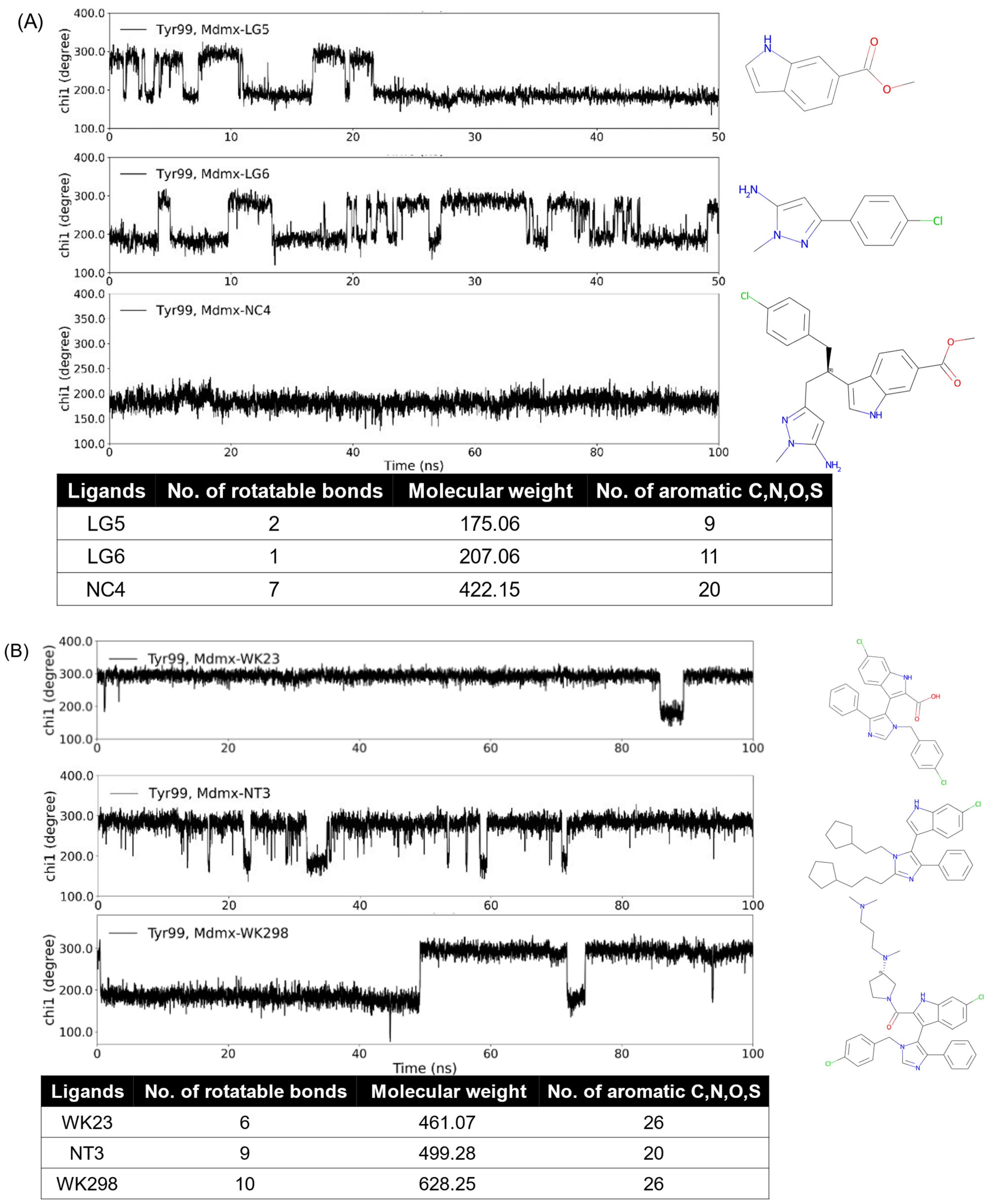
Because our interest is in the anticancer target Mdmx (mouse double minute x), which is a negative regulator of the p53 tumor suppressor [52], we designed a series of Mdmx inhibitors. MD simulations were used to study the conformational changes in the Mdmx complexes with these newly designed molecules and known Mdmx inhibitors, i.e., WK298 and WK23 [53].
In this work, all-atom MD simulations were implemented using the AMBER 20 software on GPUs [54]. The initial structures were the binding poses selected from the docking results. Each system consisted of one copy of the Mdmx protein (PDB ID: 3dab [55]) surrounded by TIP3P [56] water molecules and one chloride ion neutralizing the entire system. The partial atomic charges of the ligands were derived using the antechamber module implemented in the AMBER software package to calculate AM1-BCC charges [57,58,59]. The other force field parameters of ligands derived from the general AMBER force field (GAFF, version 2) [60] and the AMBER FF14SB force field [61] were employed to model Mdmx. Antechamber prepared residue topologies for ligands and LEaP for Mdmx.
For each system, the solvent of the MD system was first minimized using the XMIN method across 20,000 steps. All of the solutes were restrained using a harmonic potential with a force constant of 100 (kcal/mol)/Å2. The MD simulation consisted of three phases: the relaxation phase, equilibrium phase, and sampling phase. In the relaxation phase, the simulation system was heated progressively from 0 to 300 K in steps of 50 K and 5 ps each with a force constant of 2 (kcal/mol)/Å2, followed by maintaining the temperature at 300 K in the last 20 ps. After the heating steps, the system was equilibrated at 1 bar for 10 ns but without any restraints or constraints in the last 5 ns. Finally, a 100 ns MD simulation was performed for each system. In total, 10,000 frames were recorded during the production phase. Additional settings for constant volume and pressure MD simulations performed in this work are as follows: the temperature was regulated by the weak-coupling algorithm; pressure was regulated by the isotropic position scaling algorithm with the pressure relaxation time set to 1.0 ps; integration of the equations of motion was conducted at a time step of 0.5 fs for the heating steps and 2 fs for others. All bonds involving hydrogen atoms were constrained using the SHAKE algorithm in the MD simulation stages. The particle mesh Ewald (PME) procedure processed long-range electrostatic interactions.
Mdmx has two transient conformational states concerning the binding pocket, which are determined by the side-chain torsion angle of Tyr99 (χ1). The “open” and “closed” states correspond to χ1 of around 180° and 300°, respectively [55,62]. The open state yields an enlarged pocket and provides a transient subpocket. Thus, the χ1 angle of Tyr99 is an indicator of the open/closed state of Mdmx. A cluster analysis of the frames was carried out with a distance metric (RMSD of backbone atoms) using the K-means clustering algorithm. Both the representative and last frames were used to analyze the binding conformation.
3. Results
3.1. Model Performance
The PDBbind and NR-DBIND databases were processed using the protocol described in the Datasets section. We did not limit the number of holo structures or apo structures considered for the same protein. Thus, our data covered the same protein binding with different ligands. Both agonists and antagonists were used in our analysis. In some cases, a protein had more than one resolved apo structure, providing diverse conformations during the movement of this protein in the ligand-free state. The 474 holo structures in the PDBbind set and 53 holo structures in the NR-DBIND set had only one matched apo structure. The remaining holo structures had multiple apo structures deposited in the PDB database, which were tentatively retrieved (at most 10 apo structures per holo structure) to exactly determine the classification labels of the ligands. Of all apo structures (which were considered to be produced by the intrinsic flexibility of proteins), we selected the one with the maximum pocket, which was used as a reference for comparison with respective holo structures. To some extent, this analysis eliminated the cryptic pocket formed by the conformational selection.
Before modeling, both datasets were manually checked to ensure that the apo structure correctly matched the corresponding holo structure; the blastp identities for holo–apo pairs were greater than 85% for PDBbind and NR-DBIND sets. OCHEM was used to build classification models to separate inducers and non-inducers.
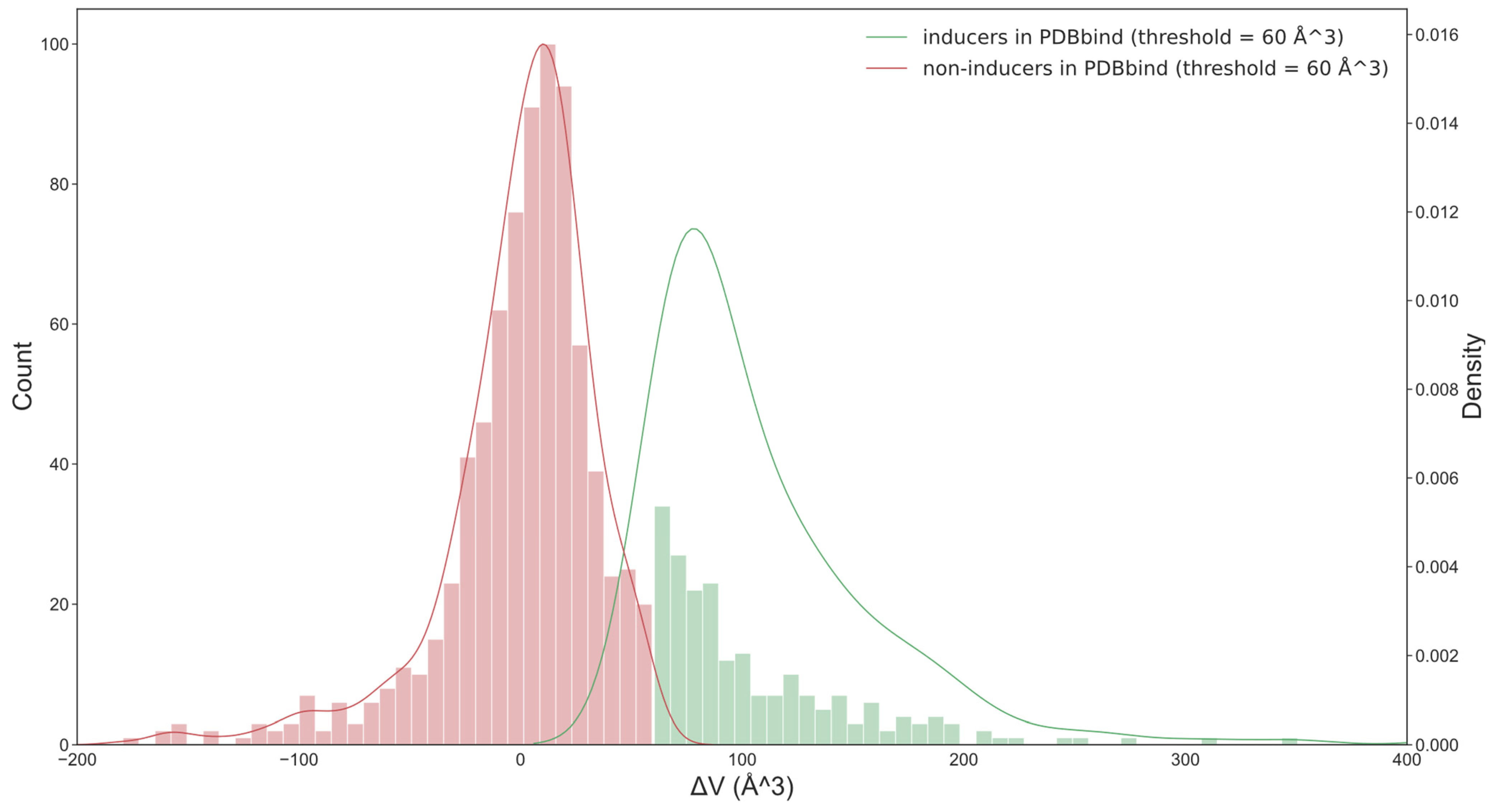
For each protein, we identified the pair with the largest differences in the volumes of apo and holo pockets. The number of pairs that had Vholo − Vapo > 0 Å3 was more than twice the number of pairs that had a negative change in volume (Figure 2). However, a small change in pocket size should not be considered a pocket opening. This could be simply pocket adaptation or pocket fluctuation. The minimum volume of the holo pocket identified by SiteMap was 41 Å3, and the minimum ligand (pyruvic acid) was 67 Å3 in size. We expected that an optimum threshold to separate inducers and non-inducers would be of similar size.
To determine an optimal threshold, we investigated different ΔV values from 20 to 100 Å3 at intervals of 10 Å3. Our assumption was that if inducers and non-inducers have different features, then an optimal threshold should correspond to the model with the highest performance.
After analyzing the performance of machine learning methods and descriptors available in OCHEM, we found that random forest (RF) [31] combined with AlogPS [36] and OEstate [34,37] (AO) descriptors provided models with higher performances on average compared to other analyzed methods and descriptors. The highest average AUC value for both sets was obtained with a threshold of 60 Å3 (Table 1). For this threshold, 132 and 93 ligands were classified as inducers for the PDBbind and NR-DBIND sets, respectively. The binding of NR ligands usually triggered large movements of NR, and thus, most of the ligands binding these proteins were likely to be inducers. Therefore, the change in the threshold did not notably change the number of inducers and non-inducers for this set. For the training set, the selection of the threshold strongly affected the ratios of inducers and non-inducers.
We had 95 types of proteins in the training set. The model was trained with diverse proteins and was tested on the test set exclusively containing nuclear receptors. It had a lower AUC accuracy for the test set as compared to that for the training set. Nevertheless, the difference in the performance was not large (AUC 0.71 vs. AUC 0.65).
3.2. Interpretation of Models
Table 2 contains the top 20 most important descriptors identified by the SHAP algorithm.
The top 20 AO descriptors were plotted in descending order of their respective importance in the model (see Supplementary Materials, Figure S1). There are several features related to heteroatoms. Sulfonyl (SddssS) and Se1C3S4ad had a positive impact, while the sulfones/sulfoxides (SdO (sulfo)) and sulfur atoms (S) were not beneficial as inducers. These results indicate that the influence of sulfur on the target property might be ambiguous and requires a deeper analysis to determine which fragment it participates in. Moreover, three nitrogen-containing substructures showed negative impacts, such as aromatic (SaaNH and SeaC3NHaa) and primary (SsNH2) amino groups. In addition, the molecular weight (MW), halogen (HALOG), phosphorus (P), and the double-bonded oxygen of carboxylic acids (SdO(acid)) also contributed to the probability that the ligand is an inducer. Interestingly, RBONDS descriptors suggested that sufficient flexibility is necessary for an inducer to adapt itself to a transient pocket, which is consistent with the conclusions of Cimermancic et al. [12] and Beglov et al. [13].
With regard to carbon atoms, descriptors such as SaaCH, SaasC, SeaC2C2aa, SeaC2C3aa, and the number of aromatic atoms (aCNOS) were derived from aromatic atoms, indicating the importance of aromatic interactions between protein and ligand to the inducer properties of ligands.
The lipophilicity of molecules (ALogPS_logP) increased the ability of molecules to act as inducers, while their solubility (ALogPS_logS) had the opposite effect. The more hydrophobic a molecule was, the more likely it was an inducer.
3.3. Analysis of Functional Groups
The OCHEM SetCompare tool [63,64,65] used a hypergeometric distribution to identify the functional groups [66] that were overrepresented in inducers and non-inducers. As shown in Table 3, sulfonic acid derivatives appeared more often in non-inducers, and sulfonamides accounted for 97% of these derivatives (179 out of 184 ligands). Note that the primary amine was favorable for non-inducers, as indicated by the descriptor SsNH2 in the previous section. Here, we observed inducers that showed a propensity to have aromatic structures substituted by tertiary amines or halogens. In addition, phosphoric and carboxylic acids were overrepresented in the inducer cohort. These features are consistent with the explanation of the model by SHAP but also offer some new clues that have not been shown before. Pyridine and five-membered heterocycles with two heteroatoms were two substructures particularly identified by SetCompare, which could be used as building blocks for inducers.
3.4. Fragment Analysis on PDBbind Set
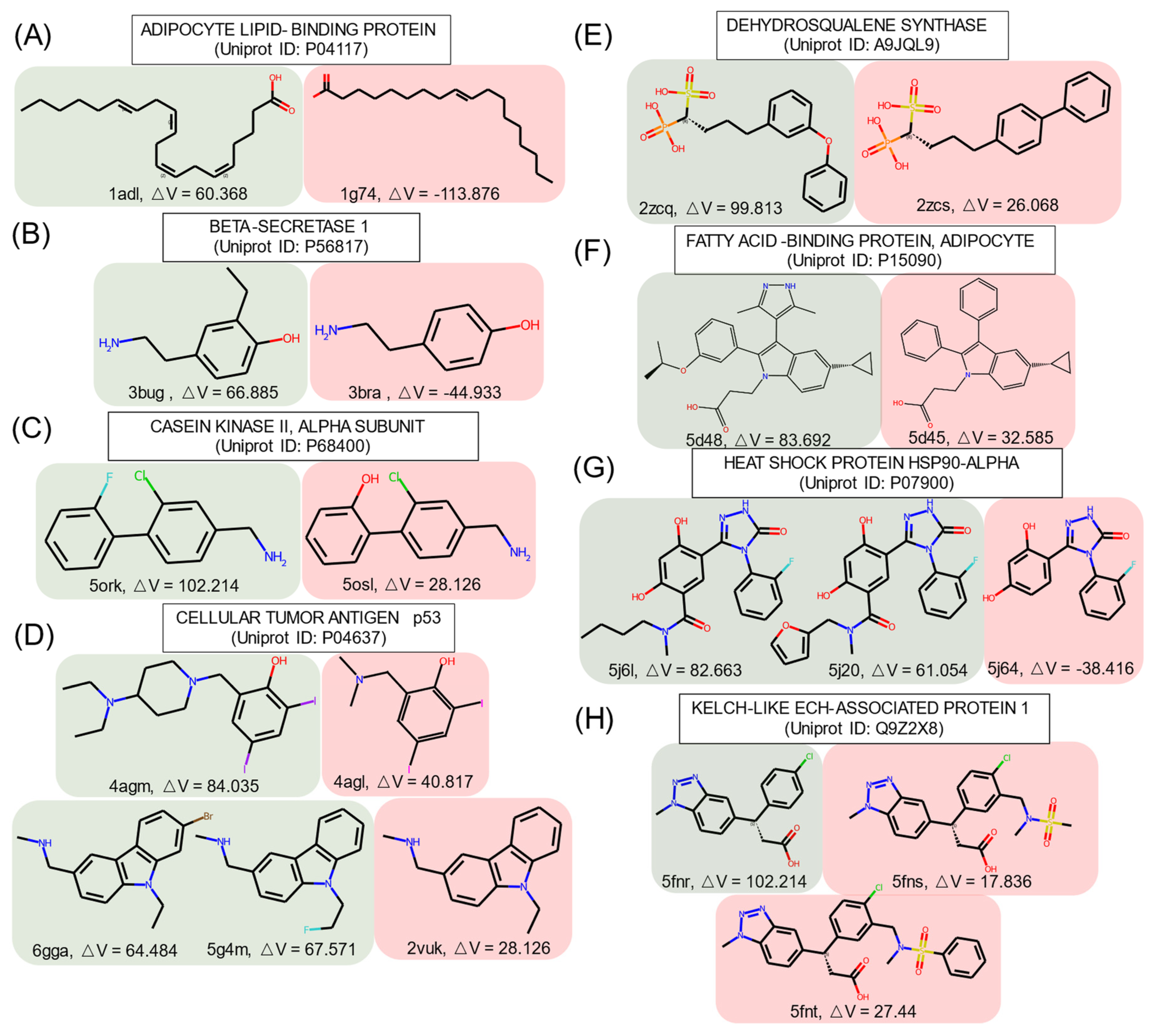
Some ligands targeting the identical protein had similar structures (similarity score ≥ 0.9, calculated on FCFP4) but had different effects on cryptic pocket opening, as shown in Figure 3, where the structures are grouped according to the effect type.
In group A, inducers preferred to have a long fatty acid chain with unsaturated bonds. A short aliphatic chain or a halogen atom turned non-inducers into inducers, as shown in groups B, C, and D. In group D, the ligand in the crystal structure with the PDB ID 4agm [67] had an additional tertiary amine and closed one of the tertiary amines forming piperidine as compared to the similar non-inducer structure of the PDB ID 4agl [67]. This emphasizes the importance of high hydrophobicity and of tertiary amines for inducers. The addition of singly bonded oxygen helped to obtain inducers in groups E and F.
In group F, replacement of the benzene ring by a pyrazole turned a non-inducer into an inducer, which is consistent with the SetCompare result, indicating that five-membered heterocycles with two heteroatoms were overrepresented in the inducers. In group G, the difference between inducers and non-inducers was the amide substructure substituted by alkyl chains or a furan ring. In group H, the inducer in the crystal structure with the PDB ID 5fnr [68] became a non-inducer with the addition of a sulfonamido group, which may suggest that sulfur atoms can decrease the propensity of a chemical structure to act as an inducer. In the crystal structure with the PDB ID 5fnt [68], the addition of another benzene ring did not influence the ability of the structure to act as an inducer.
These examples illustrate that tiny changes in chemical structures can change their ability to act as inducers or non-inducers. These changes follow the general tendencies identified using the SHAP and SetCompare algorithms.
3.5. Analysis of Mdmx Inhibitors
We are interested in the promising anticancer target Mdmx. Mdmx has two transient states, i.e., the open and closed states of Tyr99 χ1. The open state yields an enlarged pocket and provides a transient subpocket. In our previous work [69], we designed a series of Mdmx inhibitors and used MD simulations to study them and known Mdmx inhibitors. Dynamic changes in χ1 in Mdmx complexes show differences in the binding properties of Mdmx ligands. As seen from Figure 4, the increase in the number of rotatable bonds, molecular weight (MW), and aromatic atoms increased the probability of the ligands binding to the open state of Mdmx during the simulation time. Indeed, ligands LG5 and LG6 only partially bonded the Mdmx open state, while NC4, which combined both ligands and thus had increased rotatable bonds and MW as well as aromatic atoms, did so continuously (Figure 4A). Figure 4B shows three ligands with a common core structure consisting of single phenyl, indole, and pyrazole rings. Compared to WK23 and NT3, WK298 had more rotatable bonds and greater MW. The addition of the tertiary amine substructure also promoted the inducing property of WK298 [53], while WK23 [53] and NT3 were both non-inducers. Changes in the inducing propensity of ligands are thus consistent with the analysis of the descriptors and functional groups described in Section 3.3.
4. Discussion
The aim of our analysis was to determine which characteristics of small molecules were important to induce the opening of cryptic pockets, including their structural features and physical and chemical properties.
We created a training set by combining the CryptoSite [13] and PDBbind [18,19] databases and used NR-DBIND [27] as the external validation set. The volume change between the holo and apo pockets was used as a metric to identify whether the ligand was an inducer. We developed classification models by using the random forest algorithm [31] and determined that the optimum threshold to separate the two types of molecules was 60 Å3. The analysis of the developed machine learning model indicated that higher hydrophobicity and aromaticity increased the propensity of ligands to act as inducers. Inducers also tended to have tertiary amines, rather than primary or secondary amines. The impact of sulfur groups was ambiguous. Our analysis suggested that sulfones/sulfoxides substituents decreased the probability of molecules being inducers. The presence of phosphorus or halogen atoms increased the probability of molecules being inducers, as identified by the SHAP [49] and SetCompare [63,64,65] methods. Five-membered heterocycles with two heteroatoms and pyridine were overrepresented in the class of inducers, as identified by the SetCompare analysis. We also analyzed pairs of similar molecules with opposite properties and showed that small changes in the structures of molecules could result in a change in the class of compounds. Finally, we validated our findings about the inducing properties on Mdmx inhibitors. Based on the results of MD simulations, Mdmx inhibitors that induced the opening of the transient pocket possess the same features as summarized in the previous analysis of the inducers.
We also applied Lipinski’s rule of five implemented by Schrödinger software to inducers and found that majority of them (64%) were in agreement with the rules. A deep learning classification model [70] was used to evaluate the aggregation propensity of the analyzed ligands. As a result, 92.7% of the proteins in our dataset were predicted to be non-aggregators, and thus, aggregation propensity did not affect the conclusion of this work.
The proposed approach is a general one and can be adopted to analyze, e.g., peptide ligands or identify inducers of enzymes or/and signaling proteins involved in extensive protein/protein interaction networks. Since this is a statistical approach, a sufficiently large dataset should be collected from the literature to develop these models. Depending on the target class of compounds, additional descriptors could also be considered, e.g., by encoding the conformational information of peptide ligands.
This study revealed structural features that are important for molecules to induce cryptic sites in a potential protein target, and the developed model can be used to perform such an analysis of potential ligands.
The calculated models have a rather low accuracy, which can be attributed to the complexity of the analyzed property. Indeed, if the molecule has features that make it an inducer, it may not always induce a new pocket if there is already a suitable pocket for binding. Moreover, the protein should also have structural features that can enable cryptic pocket opening. The analysis provided and the features identified could be important for researchers in the design of new molecules that can open cryptic pockets. This topic is worth being further investigated together with wet-lab work in the future.
Supplementary Materials
The following are available online at https://www.mdpi.com/article/10.3390/informatics9010008/s1, Figure S1: The SHAP values calculated for the filtered descriptors; Figure S2: The distribution of pocket residues compared between holo and apo pockets for both groups of ligands.
Author Contributions
Conceptualization, Z.X. and G.P.; methodology, validation, formal analysis, investigation, data curation, writing—original draft preparation, Z.X.; writing—review and editing, Z.X., I.V.T., P.K., G.P., M.S. All authors have read and agreed to the published version of the manuscript.
Funding
This research was funded by China Scholarship Council (CSC) grant number 201706880010 for Z.X.
Data Availability Statement
All data and models are available at https://ochem.eu/model/913.
Acknowledgments
This study was partially supported by the China Scholarship Council (CSC) for providing the fellowship for Zhonghua Xia (201706880010). The authors also express gratitude to Leibniz Supercomputing Centre (LRZ) for access to the Schrödinger suite. The authors thank ChemAxon for the opportunity to use their programs in the study. We thank M. Embrechts (Rensselaer University, USA) for his help in editing the manuscript.
Conflicts of Interest
The authors declare no conflict of interest.
References
- Owens, J. Determining Druggability. Nat. Rev. Drug Discov. 2007, 6, 187. [Google Scholar] [CrossRef]
- Hopkins, A.L.; Groom, C.R. The Druggable Genome. Nat. Rev. Drug Discov. 2002, 1, 727–730. [Google Scholar] [CrossRef] [PubMed]
- Santos, R.; Ursu, O.; Gaulton, A.; Bento, A.P.; Donadi, R.S.; Bologa, C.G.; Karlsson, A.; Al-Lazikani, B.; Hersey, A.; Oprea, T.I.; et al. A Comprehensive Map of Molecular Drug Targets. Nat. Rev. Drug Discov. 2017, 16, 19–34. [Google Scholar] [CrossRef] [PubMed]
- Oprea, T.I.; Bologa, C.G.; Brunak, S.; Campbell, A.; Gan, G.N.; Gaulton, A.; Gomez, S.M.; Guha, R.; Hersey, A.; Holmes, J.; et al. Unexplored Therapeutic Opportunities in the Human Genome. Nat. Rev. Drug Discov. 2018, 17, 317–332. [Google Scholar] [CrossRef] [PubMed]
- Nagar, B.; Bornmann, W.G.; Pellicena, P.; Schindler, T.; Veach, D.R.; Miller, W.T.; Clarkson, B.; Kuriyan, J. Crystal Structures of the Kinase Domain of C-Abl in Complex with the Small Molecule Inhibitors PD173955 and Imatinib (STI-571). Cancer Res. 2002, 62, 4236–4243. [Google Scholar]
- Schindler, T.; Bornmann, W.; Pellicena, P.; Miller, W.T.; Clarkson, B.; Kuriyan, J. Structural Mechanism for STI-571 Inhibition of Abelson Tyrosine Kinase. Science 2000, 289, 1938–1942. [Google Scholar] [CrossRef] [Green Version]
- Wodicka, L.M.; Ciceri, P.; Davis, M.I.; Hunt, J.P.; Floyd, M.; Salerno, S.; Hua, X.H.; Ford, J.M.; Armstrong, R.C.; Zarrinkar, P.P.; et al. Activation State-Dependent Binding of Small Molecule Kinase Inhibitors: Structural Insights from Biochemistry. Chem. Biol. 2010, 17, 1241–1249. [Google Scholar] [CrossRef] [Green Version]
- Umezawa, K.; Kii, I. Druggable Transient Pockets in Protein Kinases. Molecules 2021, 26, 651. [Google Scholar] [CrossRef]
- Vajda, S.; Beglov, D.; Wakefield, A.E.; Egbert, M.; Whitty, A. Cryptic Binding Sites on Proteins: Definition, Detection, and Druggability. Curr. Opin. Chem. Biol. 2018, 44, 1–8. [Google Scholar] [CrossRef]
- Mizukoshi, Y.; Takeuchi, K.; Tokunaga, Y.; Matsuo, H.; Imai, M.; Fujisaki, M.; Kamoshida, H.; Takizawa, T.; Hanzawa, H.; Shimada, I. Targeting the Cryptic Sites: NMR-Based Strategy to Improve Protein Druggability by Controlling the Conformational Equilibrium. Sci. Adv. 2020, 6, eabd0480. [Google Scholar] [CrossRef]
- Kii, I.; Sumida, Y.; Goto, T.; Sonamoto, R.; Okuno, Y.; Yoshida, S.; Kato-Sumida, T.; Koike, Y.; Abe, M.; Nonaka, Y.; et al. Selective Inhibition of the Kinase DYRK1A by Targeting Its Folding Process. Nat. Commun. 2016, 7, 11391. [Google Scholar] [CrossRef] [PubMed]
- Cimermancic, P.; Weinkam, P.; Rettenmaier, T.J.; Bichmann, L.; Keedy, D.A.; Woldeyes, R.A.; Schneidman-Duhovny, D.; Demerdash, O.N.; Mitchell, J.C.; Wells, J.A.; et al. CryptoSite: Expanding the Druggable Proteome by Characterization and Prediction of Cryptic Binding Sites. J. Mol. Biol. 2016, 428, 709–719. [Google Scholar] [CrossRef] [PubMed] [Green Version]
- Kozakov, D.; Grove, L.E.; Hall, D.R.; Bohnuud, T.; Mottarella, S.E.; Luo, L.; Xia, B.; Beglov, D.; Vajda, S. The FTMap Family of Web Servers for Determining and Characterizing Ligand-Binding Hot Spots of Proteins. Nat. Protoc. 2015, 10, 733–755. [Google Scholar] [CrossRef] [Green Version]
- Beglov, D.; Hall, D.R.; Wakefield, A.E.; Luo, L.; Allen, K.N.; Kozakov, D.; Whitty, A.; Vajda, S. Exploring the Structural Origins of Cryptic Sites on Proteins. Proc. Natl. Acad. Sci. USA 2018, 115, E3416–E3425. [Google Scholar] [CrossRef] [PubMed] [Green Version]
- Clark, J.J.; Benson, M.L.; Smith, R.D.; Carlson, H.A. Inherent versus Induced Protein Flexibility: Comparisons within and between Apo and Holo Structures. PLoS Comput. Biol. 2019, 15, e1006705. [Google Scholar] [CrossRef] [Green Version]
- Evans, D.J.; Yovanno, R.A.; Rahman, S.; Cao, D.W.; Beckett, M.Q.; Patel, M.H.; Bandak, A.F.; Lau, A.Y. Finding Druggable Sites in Proteins Using TACTICS. J. Chem. Inf. Model. 2021, 61, 2897–2910. [Google Scholar] [CrossRef] [PubMed]
- Kuzmanic, A.; Bowman, G.R.; Juarez-Jimenez, J.; Michel, J.; Gervasio, F.L. Investigating Cryptic Binding Sites by Molecular Dynamics Simulations. Acc. Chem. Res. 2020, 53, 654–661. [Google Scholar] [CrossRef] [PubMed]
- Wang, R.; Fang, X.; Lu, Y.; Wang, S. The PDBbind Database: Collection of Binding Affinities for Protein−Ligand Complexes with Known Three-Dimensional Structures. J. Med. Chem. 2004, 47, 2977–2980. [Google Scholar] [CrossRef]
- Wang, R.; Fang, X.; Lu, Y.; Yang, C.-Y.; Wang, S. The PDBbind Database: Methodologies and Updates. J. Med. Chem. 2005, 48, 4111–4119. [Google Scholar] [CrossRef]
- Berman, H.M.; Westbrook, J.; Feng, Z.; Gilliland, G.; Bhat, T.N.; Weissig, H.; Shindyalov, I.N.; Bourne, P.E. The Protein Data Bank. Nucleic Acids Res. 2000, 28, 235–242. [Google Scholar] [CrossRef] [Green Version]
- Westbrook, J.D.; Shao, C.; Feng, Z.; Zhuravleva, M.; Velankar, S.; Young, J. The Chemical Component Dictionary: Complete Descriptions of Constituent Molecules in Experimentally Determined 3D Macromolecules in the Protein Data Bank. Bioinformatics 2015, 31, 1274–1278. [Google Scholar] [CrossRef] [PubMed] [Green Version]
- Altschul, S.F.; Madden, T.L.; Schäffer, A.A.; Zhang, J.; Zhang, Z.; Miller, W.; Lipman, D.J. Gapped BLAST and PSI-BLAST: A New Generation of Protein Database Search Programs. Nucleic Acids Res. 1997, 25, 3389–3402. [Google Scholar] [CrossRef] [PubMed] [Green Version]
- The PyMOL Molecular Graphics System; Version 2.4.0; Schrödinger, LLC: New York, NY, USA, 2021.
- Schrödinger Release 2020-3; Schrödinger, LLC: New York, NY, USA, 2020.
- Halgren, T. New Method for Fast and Accurate Binding-Site Identification and Analysis. Chem. Biol. Drug Des. 2007, 69, 146–148. [Google Scholar] [CrossRef]
- Halgren, T.A. Identifying and Characterizing Binding Sites and Assessing Druggability. J. Chem. Inf. Model. 2009, 49, 377–389. [Google Scholar] [CrossRef] [PubMed]
- Réau, M.; Lagarde, N.; Zagury, J.F.; Montes, M. Nuclear Receptors Database Including Negative Data (NR-DBIND): A Database Dedicated to Nuclear Receptors Binding Data Including Negative Data and Pharmacological Profile. J. Med. Chem. 2019, 62, 2894–2904. [Google Scholar] [CrossRef] [PubMed]
- Madhavi Sastry, G.; Adzhigirey, M.; Day, T.; Annabhimoju, R.; Sherman, W. Protein and Ligand Preparation: Parameters, Protocols, and Influence on Virtual Screening Enrichments. J. Comput.-Aided Mol. Des. 2013, 27, 221–234. [Google Scholar] [CrossRef] [PubMed]
- Shelley, J.C.; Cholleti, A.; Frye, L.L.; Greenwood, J.R.; Timlin, M.R.; Uchimaya, M. Epik: A Software Program for PKaprediction and Protonation State Generation for Drug-like Molecules. J. Comput.-Aided Mol. Des. 2007, 21, 681–691. [Google Scholar] [CrossRef]
- Sushko, I.; Novotarskyi, S.; Körner, R.; Pandey, A.K.; Rupp, M.; Teetz, W.; Brandmaier, S.; Abdelaziz, A.; Prokopenko, V.V.; Tanchuk, V.Y.; et al. Online Chemical Modeling Environment (OCHEM): Web Platform for Data Storage, Model Development and Publishing of Chemical Information. J. Comput.-Aided Mol. Des. 2011, 25, 533–554. [Google Scholar] [CrossRef] [Green Version]
- Breiman, L. Random Forests. Mach. Learning 2001, 45, 5–32. [Google Scholar] [CrossRef] [Green Version]
- Svetnik, V.; Liaw, A.; Tong, C.; Christopher Culberson, J.; Sheridan, R.P.; Feuston, B.P. Random Forest: A Classification and Regression Tool for Compound Classification and QSAR Modeling. J. Chem. Inf. Comput. Sci. 2003, 43, 1947–1958. [Google Scholar] [CrossRef]
- Oshiro, T.M.; Perez, P.S.; Baranauskas, J.A. How Many Trees in a Random Forest? In Proceedings of the Machine Learning and Data Mining in Pattern Recognition; Perner, P., Ed.; Springer: Berlin/Heidelberg, Germany, 2012; pp. 154–168. [Google Scholar]
- Tetko, I.V.; Tanchuk, V.Y.; Villa, A.E.P. Prediction of N-Octanol/Water Partition Coefficients from PHYSPROP Database Using Artificial Neural Networks and E-State Indices. J. Chem. Inf. Comput. Sci. 2001, 41, 1407–1421. [Google Scholar] [CrossRef] [PubMed]
- Tetko, I.V.; Tanchuk, V.Y.; Kasheva, T.N.; Villa, A.E.P. Estimation of Aqueous Solubility of Chemical Compounds Using E-State Indices. J. Chem. Inf. Comput. Sci. 2001, 41, 1488–1493. [Google Scholar] [CrossRef] [PubMed]
- Tetko, I.V.; Tanchuk, V.Y. Application of Associative Neural Networks for Prediction of Lipophilicity in ALOGPS 2.1 Program. J. Chem. Inf. Comput. Sci. 2002, 42, 1136–1145. [Google Scholar] [CrossRef]
- Kier, L.B.; Hall, L.H. An Electrotopological-State Index for Atoms in Molecules. Pharm. Res. 1990, 7, 801–807. [Google Scholar] [CrossRef] [PubMed]
- Kier, L.B.; Hall, L.H. Molecular Structure Description: The Electrotopological State; Elsevier Science: Amsterdam, The Netherlands, 1999; ISBN 9780124065550. [Google Scholar]
- Methods and Principles in Medicinal Chemistry Previous Volumes of This Series: Pharmacokinetics and Metabolism in Drug Design, Pharmacophores and Pharmacophore Searches Chirality in Drug Research Fragment-Based Approaches in Drug Discovery High-Throughput Screening in Drug Discovery Mass Spectrometry in Medicinal Chemistry Molecular Drug Properties Nuclear Receptors as Drug Targets. Available online: https://www.wiley.com/en-us/content-search?cq=Wiley%27s+Methods+and+Principles+in+Medicinal+Chemistry+Series&pq=Wiley%27s+Methods+and+Principles+in+Medicinal+Chemistry+Series (accessed on 20 November 2021).
- Hall, L.H.; Kier, L.B. Electrotopological State Indices for Atom Types: A Novel Combination of Electronic, Topological, and Valence State Information. J. Chem. Inf. Comput. Sci. 1995, 35, 1039–1045. [Google Scholar] [CrossRef]
- Shapley, L.S. A Value Fo N-Person Games; Princeton University Press: Princeton, NJ, USA, 2016; pp. 307–318. [Google Scholar]
- Lundberg, S.M.; Lee, S.-I. A Unified Approach to Interpreting Model Predictions. In Proceedings of the 30th Conference on Neural Information Processing Systems (NIPS 2017); Guyon, I., Luxburg, U.V., Bengio, S., Wallach, H., Fergus, R., Vishwanathan, S., Garnett, R., Eds.; Curran Associates, Inc.: Red Hook, NY, USA, 2017; Volume 30. [Google Scholar]
- Ribeiro, M.T.; Singh, S.; Guestrin, C. “Why Should I Trust You?”: Explaining the Predictions of Any Classifier. In Proceedings of the 22nd ACM SIGKDD International Conference on Knowledge Discovery and Data Mining; Association for Computing Machinery: New York, NY, USA, 2016; pp. 1135–1144. [Google Scholar]
- Shrikumar, A.; Greenside, P.; Kundaje, A. Learning Important Features Through Propagating Activation Differences. arXiv 2019, arXiv:1704.02685. [Google Scholar]
- Bach, S.; Binder, A.; Montavon, G.; Klauschen, F.; Müller, K.-R.; Samek, W. On Pixel-Wise Explanations for Non-Linear Classifier Decisions by Layer-Wise Relevance Propagation. PLoS ONE 2015, 10, e0130140. [Google Scholar] [CrossRef] [Green Version]
- Lipovetsky, S.; Conklin, M. Analysis of Regression in Game Theory Approach. Appl. Stoch. Models Bus. Ind. 2001, 17, 319–330. [Google Scholar] [CrossRef]
- Štrumbelj, E.; Kononenko, I. Explaining Prediction Models and Individual Predictions with Feature Contributions. Knowl. Inf. Syst. 2014, 41, 647–665. [Google Scholar] [CrossRef]
- Datta, A.; Sen, S.; Zick, Y. Algorithmic Transparency via Quantitative Input Influence: Theory and Experiments with Learning Systems. In Proceedings of the 2016 IEEE Symposium on Security and Privacy (SP), San Jose, CA, USA, 22–26 May 2016; pp. 598–617. [Google Scholar]
- Lundberg, S.M.; Erion, G.; Chen, H.; DeGrave, A.; Prutkin, J.M.; Nair, B.; Katz, R.; Himmelfarb, J.; Bansal, N.; Lee, S.-I. From Local Explanations to Global Understanding with Explainable AI for Trees. Nat. Mach. Intell. 2020, 2, 56–67. [Google Scholar] [CrossRef] [PubMed]
- Pedregosa, F.; Varoquaux, G.; Gramfort, A.; Michel, V.; Thirion, B.; Grisel, O.; Blondel, M.; Prettenhofer, P.; Weiss, R.; Dubourg, V.; et al. Scikit-Learn: Machine Learning in Python. J. Mach. Learn. Res. 2011, 12, 2825–2830. [Google Scholar]
- Rogers, D.; Hahn, M. Extended-Connectivity Fingerprints. J. Chem. Inf. Model. 2010, 50, 742–754. [Google Scholar] [CrossRef] [PubMed]
- Shvarts, A.; Steegenga, W.T.; Riteco, N.; van Laar, T.; Dekker, P.; Bazuine, M.; van Ham, R.C.; van der Houven van Oordt, W.; Hateboer, G.; van der Eb, A.J.; et al. MDMX: A Novel P53-Binding Protein with Some Functional Properties of MDM2. EMBO J. 1996, 15, 5349–5357. [Google Scholar] [CrossRef] [PubMed]
- Popowicz, G.M.; Czarna, A.; Wolf, S.; Wang, K.; Wang, W.; Dömling, A.; Holak, T.A. Structures of Low Molecular Weight Inhibitors Bound to MDMX and MDM2 Reveal New Approaches for P53-MDMX/MDM2 Antagonist Drug Discovery. Cell Cycle 2010, 9, 1104–1111. [Google Scholar] [CrossRef] [PubMed] [Green Version]
- AMBER 2020; University of California: San Francisco, CA, USA, 2020; Available online: https://ambermd.org/doc12/Amber20.pdf (accessed on 20 November 2021).
- Popowicz, G.M.; Czarna, A.; Holak, T.A. Structure of the Human Mdmx Protein Bound to the P53 Tumor Suppressor Transactivation Domain. Cell Cycle 2008, 7, 2441–2443. [Google Scholar] [CrossRef] [Green Version]
- Jorgensen, W.L.; Madura, J.D. Quantum and Statistical Mechanical Studies of Liquids. 25. Solvation and Conformation of Methanol in Water. J. Am. Chem. Soc. 2002, 105, 1407–1413. [Google Scholar] [CrossRef]
- Jakalian, A.; Bush, B.L.; Jack, D.B.; Bayly, C.I. Fast, Efficient Generation of High-Quality Atomic Charges. AM1-BCC Model: I. Method. J. Comput. Chem. 2000, 21, 132–146. [Google Scholar] [CrossRef]
- Jakalian, A.; Jack, D.B.; Bayly, C.I. Fast, Efficient Generation of High-Quality Atomic Charges. AM1-BCC Model: II. Parameterization and Validation. J. Comput. Chem. 2002, 23, 1623–1641. [Google Scholar] [CrossRef]
- Dewar, M.J.S.; Zoebisch, E.G.; Healy, E.F.; Stewart, J.J.P. Development and Use of Quantum Mechanical Molecular Models. 76. AM1: A New General Purpose Quantum Mechanical Molecular Model. J. Am. Chem. Soc. 2002, 107, 3902–3909. [Google Scholar] [CrossRef]
- Wang, J.; Wolf, R.M.; Caldwell, J.W.; Kollman, P.A.; Case, D.A. Development and Testing of a General Amber Force Field. J. Comput. Chem. 2004, 25, 1157–1174. [Google Scholar] [CrossRef] [PubMed]
- Maier, J.A.; Martinez, C.; Kasavajhala, K.; Wickstrom, L.; Hauser, K.E.; Simmerling, C. Ff14SB: Improving the Accuracy of Protein Side Chain and Backbone Parameters from Ff99SB. J. Chem. Theory Comput. 2015, 11, 3696–3713. [Google Scholar] [CrossRef] [PubMed] [Green Version]
- Popowicz, G.M.; Czarna, A.; Rothweiler, U.; Szwagierczak, A.; Krajewski, M.; Weber, L.; Holak, T.A. Molecular Basis for the Inhibition of P53 by Mdmx. Cell Cycle 2007, 6, 2386–2392. [Google Scholar] [CrossRef] [PubMed] [Green Version]
- Vorberg, S.; Tetko, I.V. Modeling the Biodegradability of Chemical Compounds Using the Online CHEmical Modeling Environment (OCHEM). Mol. Inform. 2014, 33, 73–85. [Google Scholar] [CrossRef] [Green Version]
- Tetko, I.V.; Lowe, D.M.; Williams, A.J. The Development of Models to Predict Melting and Pyrolysis Point Data Associated with Several Hundred Thousand Compounds Mined from PATENTS. J. Cheminform. 2016, 8, 2. [Google Scholar] [CrossRef] [Green Version]
- Tetko, I.V.; Novotarskyi, S.; Sushko, I.; Ivanov, V.; Petrenko, A.E.; Dieden, R.; Lebon, F.; Mathieu, B. Development of Dimethyl Sulfoxide Solubility Models Using 163 000 Molecules: Using a Domain Applicability Metric to Select More Reliable Predictions. J. Chem. Inf. Model. 2013, 53, 1990–2000. [Google Scholar] [CrossRef]
- Salmina, E.S.; Haider, N.; Tetko, I.V. Extended Functional Groups (EFG): An Efficient Set for Chemical Characterization and Structure-Activity Relationship Studies of Chemical Compounds. Molecules 2016, 21, 1. [Google Scholar] [CrossRef] [Green Version]
- Wilcken, R.; Liu, X.; Zimmermann, M.O.; Rutherford, T.J.; Fersht, A.R.; Joerger, A.C.; Boeckler, F.M. Halogen-Enriched Fragment Libraries as Leads for Drug Rescue of Mutant P53. J. Am. Chem. Soc. 2012, 134, 6810–6818. [Google Scholar] [CrossRef]
- Davies, T.G.; Wixted, W.E.; Coyle, J.E.; Griffiths-Jones, C.; Hearn, K.; McMenamin, R.; Norton, D.; Rich, S.J.; Richardson, C.; Saxty, G.; et al. Monoacidic Inhibitors of the Kelch-like ECH-Associated Protein 1: Nuclear Factor Erythroid 2-Related Factor 2 (KEAP1:NRF2) Protein–Protein Interaction with High Cell Potency Identified by Fragment-Based Discovery. J. Med. Chem. 2016, 59, 3991–4006. [Google Scholar] [CrossRef]
- Xia, Z. In Silico Structure-Based Approaches to Design Mdmx Inhibitors, Munich. Ph.D. Thesis, Technische Universität München, München, Germany, January 2022. [Google Scholar]
- Lee, K.; Yang, A.; Lin, Y.C.; Reker, D.; Bernardes, G.J.L.; Rodrigues, T. Combating Small-Molecule Aggregation with Machine Learning. Cell Rep. Phys. Sci. 2021, 2, 100573. [Google Scholar] [CrossRef]
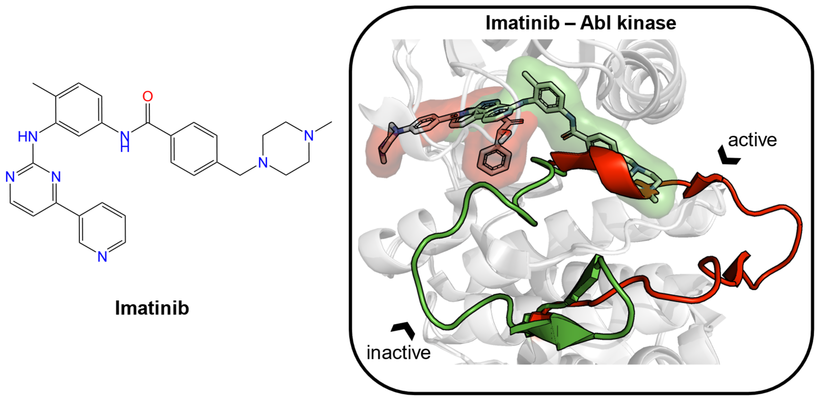
Figure 1.
The structure of imatinib is given as an example of an inducer (left). Two crystal structures of Abelson (Abl) tyrosine kinase bound with small-molecule ligands were aligned (PDB ID: 1iep, imatinib, green; PDB ID: 2v7a, PHA-739358, red). In the binding site, the major structural displacement was present in the rotation of the activation loop (residues 381–402 in Abl kinase). Imatinib (green) binds to the preformed pocket and the adjacent subpocket, which is caused by the rotation of the loop.

Figure 2.
The distribution of two classes of ligands in the PDBbind set (based on optimal threshold = 60 Å3). When the threshold was 0 Å3, the number of pairs that had Vholo − Vapo > 0 Å3 was more than twice those that had a negative change in the volume. This is inconsistent with the common knowledge that the minority of ligands have the ability to induce the opening of the pocket. The optimum threshold, which was determined in this work based on classification model performance, provided a more intuitive separation of both classes of ligands.

Figure 3.
Similar structures that are identified as inducers and non-inducers in the PDBbind set. Red: inducer; blue: non-inducer. ΔV represents the volume difference between the apo and holo pockets. The unit of △V is Å3.
Figure 3.
Similar structures that are identified as inducers and non-inducers in the PDBbind set. Red: inducer; blue: non-inducer. ΔV represents the volume difference between the apo and holo pockets. The unit of △V is Å3.

Figure 4.
MD simulations and structural features of Mdmx inhibitors. WK23 (non-inducer) and WK298 (inducer) are known Mdmx inhibitors, while the others are computationally predicted structures. The open conformation of Mdmx corresponds to Tyr99 χ1 of around 180°, while the closed one has χ1 of around 300°. Dynamic changes in χ1 in Mdmx complexes with the analyzed ligands show differences in binding properties of inducers (NC4 and WK298) as compared to the other analyzed ligands. NC4 and WK298 have more data points of χ1 around 180°, i.e., more open states; the others have more data points of χ1 around 300°, i.e., more closed states.


Table 1.
Accuracy of classification models when using different thresholds.
| Threshold (ΔV, Å3) | No. of Inducers | No. of Non- Inducers | Training Set | External Validation Set | ||||
|---|---|---|---|---|---|---|---|---|
| AUC | Balanced Accuracy | Accuracy | AUC | Balanced Accuracy | Accuracy | |||
| 0 | 759 (117) * | 317 (18) * | 0.61 | 68 | 72 | 0.56 | 56 | 81 |
| 20 | 498 (112) | 578 (23) | 0.67 | 69 | 69 | 0.51 | 51 | 76 |
| 30 | 405 (110) | 671 (25) | 0.69 | 73 | 75 | 0.59 | 59 | 78 |
| 40 | 356 (105) | 720 (30) | 0.68 | 73 | 76 | 0.54 | 54 | 67 |
| 50 | 319 (103) | 757 (32) | 0.7 | 74 | 78 | 0.58 | 58 | 75 |
| 60 | 293 (100) | 783 (35) | 0.71 | 76 | 80 | 0.65 | 65 | 80 |
| 70 | 251 (97) | 825 (38) | 0.73 | 77 | 81 | 0.60 | 60 | 73 |
| 80 | 216 (93) | 860 (42) | 0.68 | 75 | 81 | 0.67 | 67 | 79 |
| 90 | 185 (90) | 891 (45) | 0.64 | 73 | 83 | 0.57 | 57 | 64 |
| 100 | 170 (86) | 906 (49) | 0.68 | 77 | 86 | 0.60 | 60 | 64 |
* The number of inducers/non-inducers was determined by the threshold used. Numbers in brackets correspond to the validation set.
Table 2.
The most influential descriptors to classify ligands as inducers a.
| Increases Probability of Being Inducers | Decreases Probability of Being Inducers | ||
|---|---|---|---|
| Descriptor | Description | Descriptor | Description |
| SddssS |  | SdO (sulfo) |  |
| ALogPS_logP | Octanol/water partition coefficient | AlogPS_logS | Solubility in water |
| HALOG | Number of halogen atoms | SaaNH |  |
| aCNOS | The sum of aromatic C, N, O, and S atoms | SsNH2 |  |
| SaaCH |  | SeaC3NHaa |  |
| Se1C3S4ad |  | S | Number of sulfur atoms |
| SaasC |  | SdssC |  |
| SeaC2C2aa |  | ||
| RBONDS | Number of rotatable bonds | ||
| P | Number of phosphorus atoms | ||
| SeaC2C3aa |  | ||
| MW | Molecular weight | ||
| SdO (acid) |  | ||
a see SHAP values calculated for the filtered descriptor in Figure S1.
Table 3.
Functional groups overrepresented in inducers and non-inducers are listed as well as the p-value of the respective distribution.
Table 3.
Functional groups overrepresented in inducers and non-inducers are listed as well as the p-value of the respective distribution.
| Functional Group | The Ratio in Inducers (%) | The Ratio in Non-Inducers (%) | p-Value |
|---|---|---|---|
| Sulfonamides | 6.3 | 23.4 | −4.8 × 10⁻¹² |
| Sulfonic acid derivatives | 7.3 | 24.1 | −4.03 × 10⁻¹¹ |
| Halogens | 44.1 | 28.7 | 1.93 × 10⁻⁶ |
| Halogenated benzene | 28.1 | 15.1 | 1.83 × 10⁻⁶ |
| Aryl halides | 36.5 | 24.3 | 7.79 × 10⁻⁵ |
| Tertiary mixed amines | 11.5 | 4.5 | 6.66 × 10⁻⁵ |
| Five-membered heterocycles with two heteroatoms | 17.4 | 9.9 | 9.45 × 10⁻⁴ |
| Pyridine | 11.8 | 5.6 | 7.52 × 10⁻⁴ |
| Phosphorus | 13.5 | 6.8 | 6.28 × 10⁻⁴ |
| Phosphoric acids | 10.1 | 4.3 | 5.95 × 10⁻⁴ |
| Carboxylic acids | 31.6 | 21.2 | 3.62 × 10⁻⁴ |
| Aromatic halogen | 33.3 | 22.1 | 1.61 × 10⁻⁴ |
Publisher’s Note: MDPI stays neutral with regard to jurisdictional claims in published maps and institutional affiliations. |
© 2022 by the authors. Licensee MDPI, Basel, Switzerland. This article is an open access article distributed under the terms and conditions of the Creative Commons Attribution (CC BY) license (https://creativecommons.org/licenses/by/4.0/).
Share and Cite
MDPI and ACS Style
Xia, Z.; Karpov, P.; Popowicz, G.; Sattler, M.; Tetko, I.V. What Features of Ligands Are Relevant to the Opening of Cryptic Pockets in Drug Targets? Informatics 2022, 9, 8. https://doi.org/10.3390/informatics9010008
AMA Style
Xia Z, Karpov P, Popowicz G, Sattler M, Tetko IV. What Features of Ligands Are Relevant to the Opening of Cryptic Pockets in Drug Targets? Informatics. 2022; 9(1):8. https://doi.org/10.3390/informatics9010008
Chicago/Turabian StyleXia, Zhonghua, Pavel Karpov, Grzegorz Popowicz, Michael Sattler, and Igor V. Tetko. 2022. "What Features of Ligands Are Relevant to the Opening of Cryptic Pockets in Drug Targets?" Informatics 9, no. 1: 8. https://doi.org/10.3390/informatics9010008
Note that from the first issue of 2016, this journal uses article numbers instead of page numbers. See further details here.