Upsampling for Improved Multidimensional Attribute Space Clustering of Multifield Data †

Department of Mathematics and Informatics, Westfälische Wilhelms-Universität Münster, 48149 Münster, Germany
*
Author to whom correspondence should be addressed.
†
This paper is an extended version of our paper published in the 13th International Joint Conference on Computer Vision, Imaging and Computer Graphics Theory and Applications, Funchal, Portugal, 27–29 January 2018.
Information 2018, 9(7), 156; https://doi.org/10.3390/info9070156
Submission received: 11 May 2018
/
Revised: 15 June 2018
/
Accepted: 20 June 2018
/
Published: 27 June 2018
(This article belongs to the Special Issue Selected Papers from IVAPP 2018)
Abstract
:Clustering algorithms in the high-dimensional space require many data to perform reliably and robustly. For multivariate volume data, it is possible to interpolate between the data points in the high-dimensional attribute space based on their spatial relationship in the volumetric domain (or physical space). Thus, sufficiently high number of data points can be generated, overcoming the curse of dimensionality for this particular type of multidimensional data. We applies this idea to a histogram-based clustering algorithm. We created a uniform partition of the attribute space in multidimensional bins and computed a histogram indicating the number of data samples belonging to each bin. Without interpolation, the analysis was highly sensitive to the histogram cell sizes, yielding inaccurate clustering for improper choices: Large histogram cells result in no cluster separation, while clusters fall apart for small cells. Using an interpolation in physical space, we could refine the data by generating additional samples. The depth of the refinement scheme was chosen according to the local data point distribution in attribute space and the histogram’s bin size. In the case of field discontinuities representing sharp material boundaries in the volume data, the interpolation can be adapted to locally make use of a nearest-neighbor interpolation scheme that avoids averaging values across the sharp boundary. Consequently, we could generate a density computation, where clusters stay connected even when using very small bin sizes. We exploited this result to create a robust hierarchical cluster tree, apply our technique to several datasets, and compare the cluster trees before and after interpolation.
1. Introduction
Visualization of multivariate volume data has become a common, yet still challenging task in scientific visualization. Datasets come from traditional scientific visualization applications such as numerical simulations, see VisContest 2008 [1], or medical imaging, see VisContest 2010 [2]. While looking into individual attributes can be of high interest, the full phenomena are often only captured when looking into all attributes simultaneously. Consequently, visualization methods shall allow for the investigation and analysis of the multidimensional attribute space. The attribute space may consist of measured and/or simulated attributes as well as derived attributes including statistical properties (e.g., means and variances) or vector and tensor field properties (e.g., divergence, finite time Lyupanov exponent, and diffusion tensor eigenvalues). Hence, we are facing a multidimensional data analysis task, where dimension here refers to the dimensionality of the attribute space.
Multidimensional data analysis typically requires some automatic components that need to be used to produce a visual encoding. Typical components are clustering approaches or projections from higher-dimensional spaces into 2D or 3D visual spaces. Often, clustering and projections are combined to produce a visualization of a clustering result. The clustering approach shall be applied first to produce high-dimensional clusters, which can be used as an input for an improved projection. Unfortunately, clustering in a high-dimensional space faces the problem that points belonging to the same cluster can be rather far apart in the high-dimensional space. This observation is due to the curse of dimensionality, a term coined by Bellman [3]. It refers to the fact that there is an exponential increase of volume when adding additional dimensions.
The impact of the curse of dimensionality on practical issues when clustering high-dimensional data is as follows: Clustering approaches can be categorized as being based on distances between data points or being based on density estimates. However, only distance-based clustering algorithms can effectively detect clusters of arbitrary shape. Distance-based clustering approaches require local density estimates, which are typically based on space partitioning (e.g., over a regular or an adaptive grid) or on a kernel function. Both grid-based and kernel-based approaches require the choice of an appropriate size of locality for density estimation, namely, the grid cell size or the kernel size, respectively. Using a too large size leads to not properly resolving the clusters such that clusters may not be separated. Hence, a small size is required. However, due to the curse of dimensionality, clusters fall apart when using a too small size and one ends up with individual data points rather than clusters thereof.
Attribute spaces of multivariate volume data are a specific case of multidimensional data, as the unstructured data points in attribute space do have a structure when looking into the corresponding physical space. We propose to make use of this structure by applying interpolation between attribute-space data points whose corresponding representations in physical space exhibit a neighbor relationship. Thus, the objective of the paper is to develop a grid-based multifield clustering approach, which is robust to the grid cell size and is free of any density threshold.
The contributions of the paper include: generation of sufficiently high number of multifield data points to overcome the curse of dimensionality, applying a threshold-free grid-based technique for computing a hierarchical cluster tree, and visualizing the clustering results using coordinated views. The present paper extends our previous work [4] by a detailed discussion of adaptive data upsampling in the presence of sharp material boundaries or missing values, which is a typical case in many applications, e.g., for geophysical datasets. We include a new case study using climate simulation data, demonstrate the effect of adaptive interpolation in the land–sea border regions, and properly handle the varying spatial grid cells’ areas.
The overall approach presented in this paper takes as input a multivariate volume dataset. First, it applies an interpolation scheme to upsample the attribute space, see Section 4 for the main idea, Section 5 for an improved computation scheme, and Section 6 for an amendment to handle sharp material boundaries. The upsampled attribute space is then clustered using a hierarchical density-based clustering approach, see Section 3. Based on the clustering result, Section 7 describes how a combined visual exploration of physical and attribute space using coordinated views can be employed. The results of the approach are presented in Section 8 and its properties are discussed in Section 9. It is shown that our approach manages to produce high-quality clustering results without the necessity of tweaking the grid cell size or similar. We also document that comparable results cannot be obtained when clustering without the proposed interpolation step. The linked volume visualization, therefore, reflects the phenomena in the multivariate volume data more reliably.
2. Related Work
2.1. Multivariate Volume Data Visualization
Traditionally, spatial data visualization focuses on one attribute, which may be scalar, vector, or tensor-valued. In the last decade, there was an increase on attempts to generalize the visualization methods to multivariate volume data that allow for the visual extraction of multivariate features. Sauber et al. [5] suggested using multigraphs to generate combinations of multiple scalar fields, where the number of nodes in the graph increase exponentially with the number of dimensions. Similarly, Woodring and Chen [6] allowed for boolean set operations of scalar field visualization. In this context, Akiba and Ma [7] and Blaas et al. [8] were the first to use sophisticated visualization methods and interaction in the multi-dimensional attribute space. Akiba and Ma [7] suggested a tri-space visualization that couples parallel coordinates in attribute space with volume rendering in physical space in addition to one-dimensional plots over time. Blaas et al. [8] used scatter plots in attribute space, where the multi-dimensional data is projected into arbitrary planes. Daniels II et al. [9] presented an approach for interactive vector field exploration by brushing on a scatterplot of derived scalar properties of the vector field, i.e., a derived multivariate attribute space. However, their interactive attribute space exploration approach does not scale to higher-dimensional attribute spaces. Our work utilized the coordinate view concept by linking the physical volume rendering, the attribute space embedding in the form of parallel coordinates, and the computed clustering tree representation.
Maciejewski et al. [10] developed multi-dimensional transfer functions for direct volume rendering using 2D and 3D histograms and density-based clustering within these histograms. Since interactions with the histograms are necessary for visual analysis of the data, their approach is restricted to attribute spaces of, at most, three dimensions. Linsen et al. [11,12] proposed an approach that can operate on multivariate volume data with higher-dimensional attribute spaces. The attribute space is clustered using a hierarchical density-based approach and linked to physical-space visualization based on surface extraction. Recently, the approach was extended by Dobrev et al. [13] to an interactive analysis tool incorporating direct volume rendering. Dobrev et al. showed that the generated clustering result is often not as desired and propose interactive means to fix the clustering result. In this paper, we use the same clustering approach, see Section 3, and show how we can improve the results with the methods proposed here.
2.2. Clustering
Cluster analysis divides data into meaningful or useful groups (clusters). Clustering algorithms can be categorized with respect to their properties of being based on partitioning, hierarchical, based on density, or based on grids [14,15]. In partitioning methods, datasets are divided into k clusters and each object must belong to exactly one cluster. In hierarchical methods, datasets are represented using similarity trees and clusters are extracted from this hierarchical tree. In density-based methods, clusters are a dense region of points separated by low-density regions. In grid-based methods, the data space is divided into a finite number of cells that form a grid structure and all of the clustering operations are performed on the cells.
Hartigan [16,17] first proposed identifying clusters as high density clusters in data space. Wong and Lane [18] defined neighbors for each data point in data space and use the kth nearest neighbors to estimate density. After defining dissimilarity between neighboring patterns, a hierarchical cluster tree is generated by applying a single-linkage algorithm. In their paper, they show that the high density clusters are strongly consistent. However, they do not examine modes of the density function.
Ester et al. [19] introduced the DBSCAN algorithm. The first step of the DBSCAN algorithm is to estimate the density using an -neighborhood (such as a spherical density estimate). Second, DBSCAN selects a threshold level set and eliminates all points with density values less than . Third, a graph is constructed based on the two parameters and . Finally, high density clusters are generated by connected components of the graph. The drawback is the need to define appropriate parameters. Hinneburg and Keim introduced the DENCLUE approach [20], where high density clusters are identified by determining density attraction. Hinneburg et al. further introduced the HD-Eye system [21] that uses visualization to find the best contracting projection into a one- or two-dimensional space. The data are divided based on a sequence of the best projections determined by the high density clusters. The advantage of this method is that it does not divide regions of high density.
Ankerst et al. [22] introduced the OPTICS algorithm, which computes a complex hierarchical cluster structure and arranges it in a linear order that is visualized in the reachability plot. Stuetzle [23] also used a nearest-neighbor density estimate. A high density cluster is generated by cutting off all minimum spanning tree edges with length greater than a specific parameter (depending on the level-set value of the density function). Stuetzle and Nugent [24] proposed constructing a graph whose vertices are patterns and whose edges are weighted by the minimum value of the density estimates along the line segment connecting the two vertices. The disadvantage of this hierarchical density-based approach is that the hierarchical cluster tree depends on a threshold parameter (level-set value) that is difficult to determine.
We used a hierarchical density-based approach that computes densities over a grid. The main advantage of our approach is the direct identification of clusters without any threshold parameter of density level sets. Moreover, it is quite efficient and scales well. The main idea of the approach is described in Section 3. For a detailed analysis and comparison to other clustering approaches, which is beyond the scope of this paper, we refer to Reference [25].
2.3. Interpolation in Attribute Space
Our main idea was based on interpolation in attribute space, which is possible due to a meaningful neighborhood structure in physical space that can be imposed onto the attribute space. Similar observations have been used in the concept of continuous scatterplots [26,27,28,29,30]. Continuous scatterplots generalize the concept of scatterplots to the visualization of spatially continuous input data by a continuous and dense plot. The high-dimensional histograms we created can be regarded as a generalization of the 2D continuous histograms created by Bachthaler and Weiskopf [26]. It is a more difficult problem to compute continuous histograms in higher-dimensional spaces. However, in the end, we only need a discrete sampling of the continuous histogram. Hence, our computations did not aim at computing continuous histograms, but rather stick to operating on a discrete setting.
3. Clustering
We present a hierarchical density cluster construction based on nonparametric density estimation using multivariate histograms. Clusters can be identified without any threshold parameter of density level sets. Let the domain of the attribute space be given in form of a d-dimensional hypercube, i.e., a d-dimensional bounding box. To derive the density function, we spatially subdivide the domain of the dataset into cells (or bins) of equal shape and size. Thus, the spatial subdivision is given in form of a d-dimensional regular structured grid with equidistant d-dimensional grid points, i.e., a d-dimensional histogram. For each bin of the histogram, we count the number of sample points lying inside. The multivariate density function is estimated by the formula
for any x within the cell, where n is the overall number of data points, is the number of data points inside the bin, and is the area of the d-dimensional bin. As the area is equal for all bins, the density of each bin is proportional to the number of data points lying inside the bin. Hence, it suffices to just operate with those numbers .
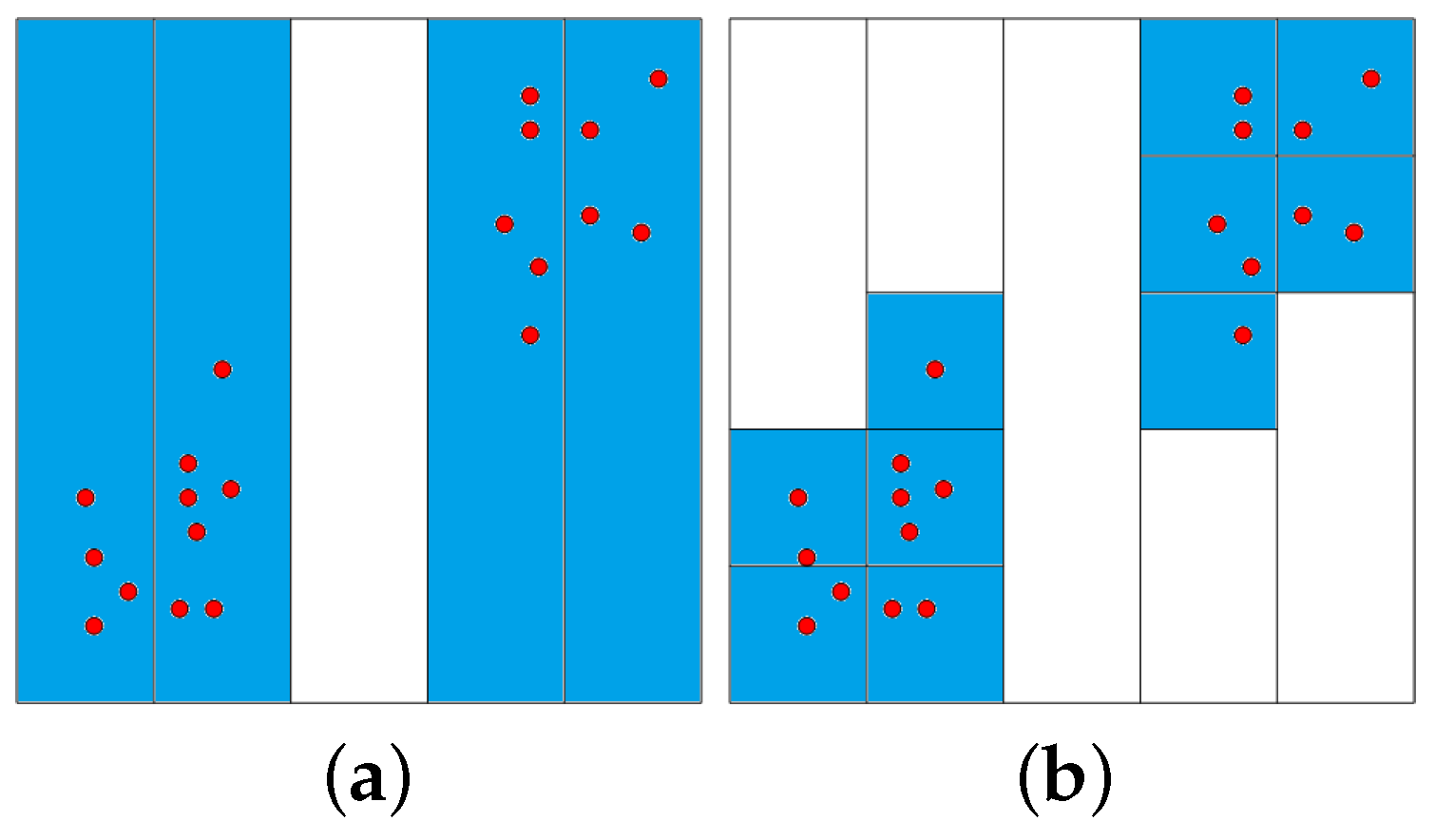
To estimate all non-empty bins, we use a partitioning algorithm that iterates through all dimensions. Figure 1 illustrates the partition process for a two-dimensional dataset: The first dimension is divided into 5 equally-sized intervals on the left-hand side of Figure 1. Only four non-empty intervals are obtained. These intervals are subsequently divided into the second dimension, as shown on the right-hand side of Figure 1. The time complexity for partitioning the data space is , i.e., it can handle both datasets with many samples n and datasets with high dimensionality d.
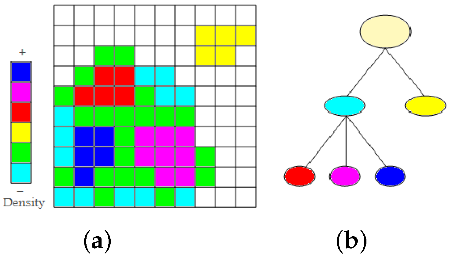
Given the d-dimensional histogram, clusters are defined as largest sets of neighboring non-empty bins, where neighboring refers to sharing a common vertex. To detect higher-density clusters within each cluster, we remove all cells containing the minimum number of points in this cluster and detect among the remaining cells, again, largest sets of neighboring cells. This step may lead to splitting of a cluster into multiple higher-density clusters. This process is iterated until no more clusters split. Recording the splitting information, we obtain a cluster hierarchy. Those clusters that do not split anymore represent local maxima and are referred to as mode clusters. Figure 2a shows a set of non-empty cells with six different density levels in a two-dimensional space. First, we find the two low-density clusters as connected components of non-empty cells. They are represented in the cluster tree as immediate children nodes of the root node (cyan and yellow), see Figure 2b. From the cluster colored cyan, we remove all minimum density level cells (cyan). The cluster remains connected. Then, we again remove the cells with minimum density level (green). The cluster splits into three higher-density clusters (red, magenta, and blue). They appear as children nodes of the cyan node in the cluster tree. As densities are given in form of counts of data points, they are always natural numbers. Consequently, we cannot miss any split of a density cluster when iterating over the natural numbers (from zero to the maximum density). The time complexity to create a hierarchical density cluster tree is , where m is the number of non-empty cells.
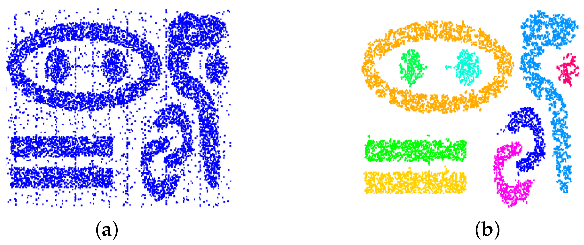
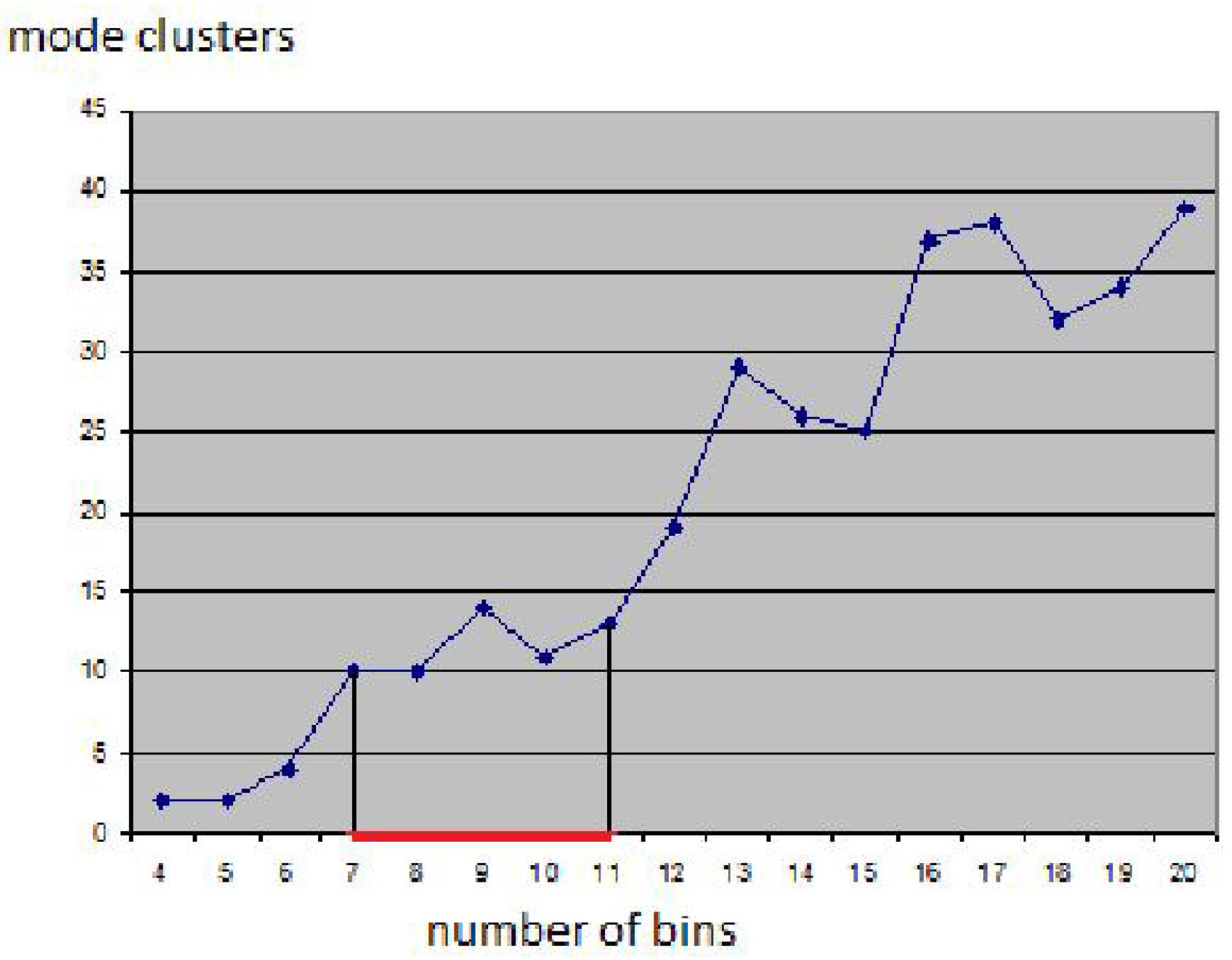
Figure 3 shows that the clustering approach is capable of handling clusters of any shape and that it is robust against changing cluster density and noise. Noise has been handled by removing all cells with a number of sample points smaller than a noise threshold. The dataset is a synthetic one [31]. Figure 4 shows the visualization of a cluster hierarchy for the “out5d” dataset with 16,384 data points and five attributes, namely, spot (SPO), magnetics (MAG), potassium (POS), thorium (THO), and uranium (URA), using a projection in optimized 2D star coordinates [25]. The result seems feasible and all clusters were found without defining any density thresholds, but the choice of the bin size had to be determined empirically. Figure 5 shows how sensitive the result is to the bin size: Using smaller bin sizes merges some clusters, while using larger sizes makes clusters fall apart. The result in Figure 4 was obtained using the heuristic that cluster numbers only vary slowly close to the optimal bin size value (area marked red in Figure 4). However, in practice, one would not generate results for the entire range of possible bin sizes for being able to apply this heuristic. Instead, one would rather use a trial-and-error approach, not knowing how reliable the result is.
4. Interpolation
Let the attribute values of the multivariate volume data be given at points , , in physical space. Moreover, let , , be the attribute values at . Then, the points exhibit some neighborhood relationship in physical space. Typically, this neighborhood information is given in the form of grid connectivity, but, even if no connectivity is given, meaningful neighborhood information can be derived in physical space by looking at distances (e.g., nearest neighbors or natural neighbors). Based on this neighborhood information, we can perform an interpolation to reconstruct a continuous multivariate field over the volumetric domain. In the following, we assume that the points are given in structured form over a regular (i.e., rectangular) hexahedral grid. Thus, the reconstruction of a continuous multivariate field can be obtained by simple trilinear interpolation within each cuboid cell of the underlying grid. More precisely: Let be a point inside a grid cell with corner points , , and let be the local Cartesian coordinates of within the cell. Then, we can compute the attribute values at by
for all attributes (). In attribute space, we obtain the point , which lies within the convex hull of the set of points , .
Now, we want to use the interpolation scheme to overcome the curse of dimensionality when creating the d-dimensional density histogram. Using the trilinear interpolation scheme, we reconstruct the multivariate field within each single cell, which corresponds to a reconstructed area in attribute space. The portion by which the reconstructed area in attribute space falls into a bin of the d-dimensional density histogram defines the amount of density that should be added to the respective bin of the histogram. Under the assumption that each grid cell has volume , where c is the overall number of grid cells, one should add the density to the respective bin of the histogram. However, we propose to not compute r exactly for two reasons: First, the computation of the intersection of a transformed cuboid with a d-dimensional cell in a d-dimensional space can be rather cumbersome and expensive. Second, the resulting densities that are stored in the bins of the histogram would no longer be natural numbers. The second property would require us to choose density thresholds for the hierarchy generation. How to do this without missing cluster splits is an open question.
Our approach is to approximate the reconstructed multivariate field by upsampling the given dataset. This discrete approach is reasonable, as the output of the reconstruction/upsampling is, again, a discrete structure, namely a histogram. We just need to assure that the rate for upsampling is high enough such that the histogram of an individual grid cell has all non-empty bins connected. Thus, the upsampling rate depends on the size of the histogram’s bins. Moreover, if we use the same upsampling rate for all grid cells, density can still be measured in the form of the number of (upsampled) data points per bin. Hence, the generation of the density-based cluster hierarchy still works as before.
Figure 6 shows the impact of upsampling in the case of a 2D physical space and a 2D attribute space, i.e., for a transformed 2D cell with corners , , and a histogram with dimensions. Without the upsampling, the non-empty bins of the histogram are not connected. After upsampling, the bins between the original non-empty bins have also been filled and the 2D cell represents a continuous region in the 2D attribute space.
When performing the upsampling for all cells of the volumetric grid, we end up with a histogram, where all non-empty cells are connected. Hence, we have overcome the curse of dimensionality. On such a histogram, we can generate the density-based cluster hierarchy without the effect of clusters falling apart.
5. Adaptive Scheme
To assure connectivity of non-empty histogram bins, we have to upsample in some regions more than in other regions. As we want to have a global upsampling rate, some regions may be oversampled. Such an oversampling is not a problem in terms of correctness, but a waste of computation time. To reduce computation time, we propose to use an adaptive scheme for upsampling. Since we are dealing with cuboid grid cells, we can adopt an octree scheme: Starting with an original grid cell, we upsample with a factor of two in each dimension. The original grid cell is partitioned into eight subcells of equal size. If the corners of a subcell S all correspond to one and the same histogram bin B, i.e., if fall into the same bin B for all corners , then we can stop the partitioning S. If the depth of the octree is and we stop partitioning S at depth , we increase the bin count (or density, respectively) of bin B by . If the corners of a subcell S do not correspond to the same histogram bin, we continue with the octree splitting of S until we reach the maximum octree depth .
Memory consumption is another aspect that we need to take into account, since multivariate volume data per se are already quite big and we further increase the data volume by applying an upsampling. However, we can march through each original cell, perform the upsampling for that cell individually, and immediately add data point counts to the histogram. Hence, we never need to store the upsampled version of the full data. However, we need to store the histogram, which can also be substantial as bin sizes are supposed to be small. We handle the histogram by storing only non-empty bins in a dynamic data structure.
6. Nearest-Neighbor Interpolation at Sharp Material Boundaries
Some data such as the ones stemming from medical imaging techniques may exhibit sharp material boundaries. It is inappropriate to interpolate across those boundaries. In practice, such abrupt changes in attribute values may require our algorithm to execute many interpolation steps. To avoid interpolation across sharp feature boundaries, we introduce a user-specified parameter that defines sharp boundaries. As this is directly related to the number of interpolation steps, the user just decides on the respective maximal number of interpolation steps . If two neighboring points in physical space have attribute values that lie in histogram cells that would not get connected after interpolation steps, performing some few interpolation steps across sharp material boundary may introduce noise artifacts leading to artificial new clusters. One option to avoid generation of artificial noise is to perform no interpolation between those points.
Geophysical datasets, e.g., representing satellite measurements or climate simulations, usually contain 2D scalar fields sampled on the Earth surface or 3D fields having vertical stratification. Many geophysical fields have a natural discontinuity along the land–ocean border and therefore should not be smoothly interpolated across this border. It is also common to have fields with missing values, which may stem from failed measurements or may be a natural property of the field. Thus, many geophysical fields, e.g., drainage, soil wetness or surface temperature of water, are defined only for land or only for sea regions. Usual smooth (e.g., bi- or trilinear) interpolation within the cells attached to grid nodes with missing values in any of the fields is technically impossible. Moreover, a distinct (invalid) numerical value can be used instead of a missing value marker in some datasets. A smooth interpolation may then produce unexpected unphysical results. The amount of cells with at least one missing value or sharp boundary in any field from the dataset can be of any size, i.e., they may be a substantial part of the overall dataset. If we decide to perform no upsampling in all such cells as suggested above, we may exclude a significant portion of data from analysis.
Hence, we propose to adjust our upsampling procedure in case cells with at least one missing value or sharp boundary exist according to the following rule: The fields with no discontinuities or missing values are interpolated using a smooth interpolation scheme as before, while a nearest-neighbor interpolation is applied to those fields with missing values or having big jumps in their values. Hence, the upsampling in the multi-dimensional attribute space of the fields is applied to all samples, while the upsampling scheme (smooth or nearest-neighbor) depends on the characteristics of the underlying field/attribute.
7. Interactive Visual Exploration
After having produced a clustering result of the attribute space that does not suffer from the curse of dimensionality, it is, of course, of interest to also investigate the clusters visually in physical and attribute space. Hence, we want to visualize, which regions in physical space belong to which attribute space cluster and what are the values of the respective attributes.
For visualizing the attribute space clusters we use the cluster tree, see Figure 2b, and visualize it in a radial layout, see Figure 7 (lower row). The cluster tree functions as an interaction widget to select any cluster or any set of clusters. The properties of the selected clusters can be analyzed using a linked parallel coordinates plot that shows the function values in attribute space, see Figure 8 (middle row).
The distribution of the selected clusters in volume space can be shown in a respective visualization of the physical space. We support both a direct volume rendering approach and a surface rendering approach. The 3D texture-based direct volume renderer takes as input only the density values stemming from the clustering step and the cluster indices, see [13]. Similarly, we extract boundary surfaces of the clusters using a standard isosurface extraction method, see Figure 8 (bottom). We illuminate our renderings using normals that have been derived as gradients from the density field that stems from the clustering approach.
8. Results
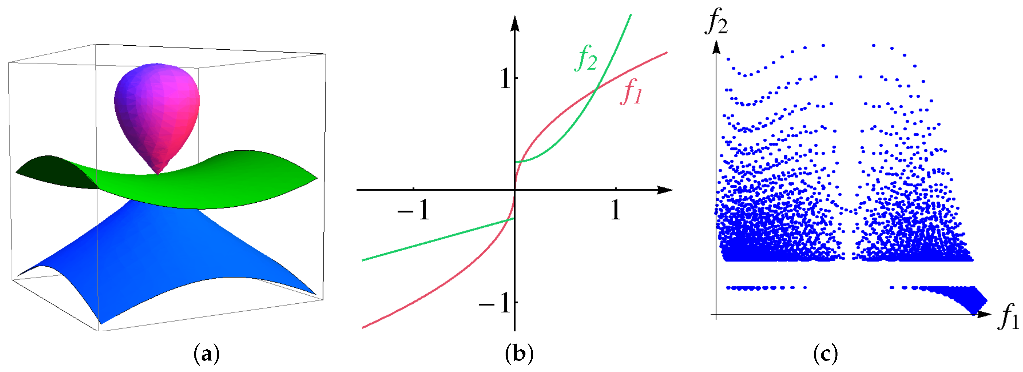
First, we demonstrate on a simple scalar field example how our approach works and show that the discrete histogram of interpolated data approaches the continuous analogon as the interpolation depth increases. Let scalar field be defined as follows:
where r stands for the Euclidean distance to the center of domain , see Figure 9a. The continuous histogram can be computed using the relation
which leads to
The continuous histogram is plotted in Figure 9b. The continuous data are clearly separated into two clusters, which represent the interior of a sphere and the background in physical space. However, when sampling the field at regular samples in the physical domain. the use of 100 bins in the attribute space leads to the effect that the sphere cluster breaks into many small parts. In Figure 7, we demonstrate how our interpolation approach corrects the histogram (upper row) and the respective cluster tree (lower row). Without upsampling or with a low-rate upsampling (), the corresponding histograms contain multiple local minima. Therefore, a non-vanishing density threshold is required for a correct identification of two analytically designed clusters. However, a reliable choice of such a threshold is difficult in a general set-up and thus should be avoided. As the upsampling depth grows, the resulting discrete histograms approach the shape of the continuous one. Depth is needed to converge to the correct result of the two clusters without the need of any density threshold.
Second, we design a volumetric multi-attribute dataset, for which the ground truth is known, show how the size of bins affects the result of the clustering procedure and demonstrate that interpolation helps to resolve the issue. Given physical domain , we use the following algebraic surfaces
see Figure 10a. We construct the distributions of two attributes as functions of algebraic distances to the surfaces above, i.e.,
Functions are chosen to have a discontinuity or a large derivative at the origin, respectively, see Figure 10b. Thus, the surfaces are cluster boundaries in the physical space. The distribution of the attribute values is shown in a 2D scatterplot in Figure 10c when sampling over a regular grid with nodes. The data represent four clusters. Using 10 bins for each attribute to generate the histogram is not enough to separate all clusters resulting in a cluster tree with only two clusters as shown in Figure 8 (upper row). A larger number of bins is necessary. When increasing the number of bins to 30 for each attribute clusters fall apart due to the curse of dimensionality, which leads to a noisy result with too many clusters, see Figure 8 (middle row). However, applying four interpolation steps fixes the histogram. Then, the cluster tree has the desired four leaves and the boundary for all four clusters are correctly detected in physical space, see Figure 8 (lower row).
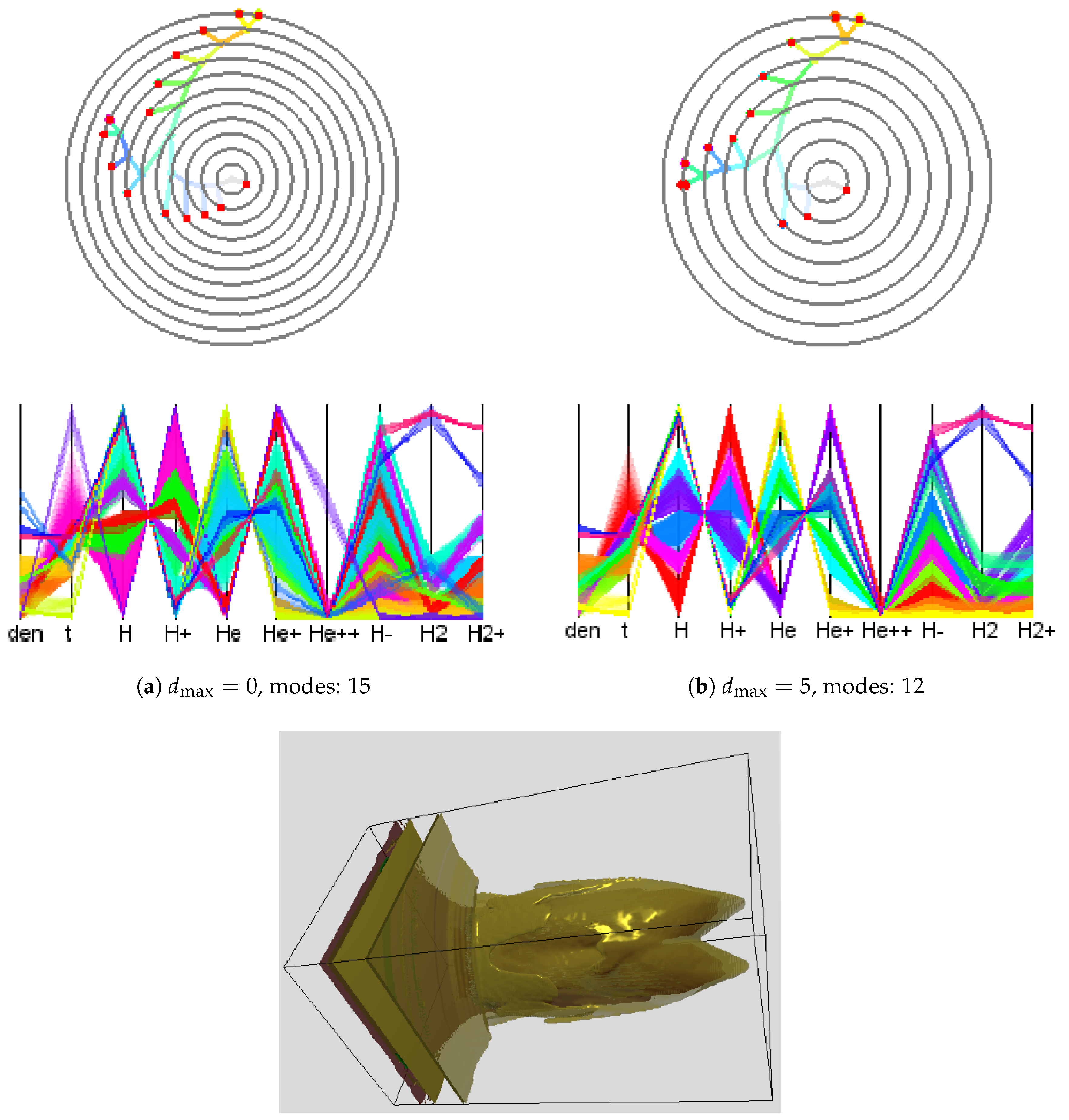
Next, we applied our methods to the simulation-based dataset provided in the 2008 IEEE Visualization Design Contest [1] and quantified the gain of (modified) adaptive upsampling. We picked time slice 75 of this ionization front instability simulation. We considered the 10 scalar fields (mass density, temperature, and mass fractions of various chemical elements). What is of interest in this dataset are the different regions of the transition phases between atoms and ions of hydrogen (H) and helium (He). To reduce computational efforts, we used the symmetry of the data with respect to the and the planes and restricted consideration to data between and localizing the front. When applying the clustering approach to the original attribute space using a 10-dimensional histogram with 10 bins in each dimension, we obtained a cluster tree with 15 mode clusters. The cluster tree and the corresponding parallel coordinates plot are shown in Figure 11a. Not all of the clusters are meaningful, since some of them appear as a result of data discretization or a sub-optimal choice of the histogram bin size. These mode clusters are not clearly separated when observing the parallel coordinates plot, see, for example, axis in Figure 11a. After applying our approach with , such clusters were merged leading to 12 modes and a simplified cluster tree. Results are shown in Figure 11b. The timings of adaptive and non-adaptive upsampling for different interpolation depths are given in Table 1. “Modified adaptive” upsampling refers to the approach with no upsampling across sharp material boundaries, see Section 6. The adaptive schemes lead to a significant speed up (up to one order of magnitude). All numerical tests presented in this section were performed on a PC with an Intel Xeon 3.20 GHz processor.
Skipping the voxels with sharp material boundaries or missing values is reasonable only if the fraction of such voxels is low. In our next experiment we used a dataset (courtesy of Max-Planck-Institute for Meteorology) representing a climate simulation which is a spin-up of a preindustrial climate state (approximately 1850 AD). It covers a period of 100 years storing monthly mean data values. The full dataset consists of time steps at which many scalar fields either volumetric or at the Earth surface are recorded. We picked two 2D fields surface temperature and surface runoff and drainage sampled at a regular (longitude-latitude) grid of size at a single time step. The field surface temperature is globally defined and has values between 210.49 K and 306.26 K, see Figure 12a. The field surface runoff and drainage contains dimensionless values between 0 kg/ms and kg/ms and has non-vanishing values only in the land regions, see Figure 12b. Thus, the field has sharp boundaries along the cost line. Due to the low resolution of the spatial grid, about of the grid cells contain a part of the land–sea border, see Figure 12c. A smooth interpolation of the field surface runoff and drainage within these cells does not correspond to the discontinuity observed in the real world. A nearest-neighbor interpolation a better and more natural choice for these grid cells. For the other grid cells, bi-linear interpolation is chosen. Moreover, the globally smooth field surface temperature can be upsampled using a bi-linear interpolation scheme for all grid cells within the whole domain.
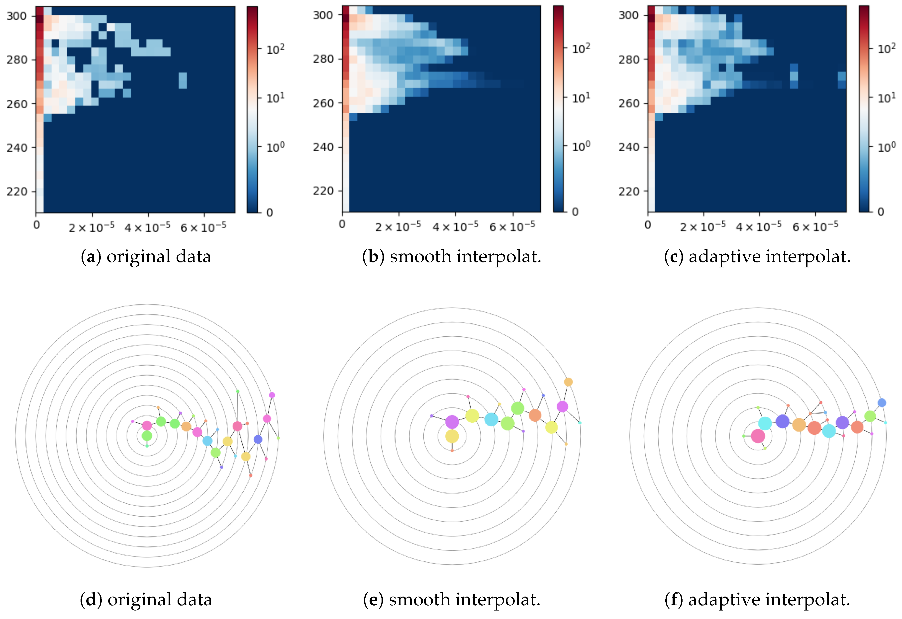
In this experiment, we used 25 bins in each dimension for all histograms. Due to the variation of the surface element area, we weighted the data samples by the cosine of their latitude when accumulating them in a histogram. Figure 13a shows a 2D histogram computed for the original data, i.e., without upsampling. The first column of the histogram corresponds to the regions with vanishing surface runoff and drainage including oceans and ordinary and polar deserts. The histogram data are noisy, which is reflected in the corresponding cluster tree of depth 13 with 28 nodes shown in Figure 13d. When applying a smooth bi-linear interpolation to both fields globally with the upsampling depth equal to four in each dimension, the resulting histogram shown in Figure 13b becomes over-smoothed. In particular, the small separated cluster on the right-hand side in Figure 13a has been merged with the main cluster in Figure 13b and is not even anymore a local maximum. The cluster tree constructed for this histogram has depth 9 and contains 19 nodes, see Figure 13e. A histogram for the data upsampled with the nearest-neighbor interpolation of field surface runoff and drainage in the coastal region cells is shown in Figure 13c. The corresponding cluster tree has depth 9 and contains 22 nodes. Thus, adaptive interpolation allows for reducing noise artifacts in the histogram data but avoids over-smoothing the data. Thus, the structure of the resulting cluster tree is simplified without losing important clusters.
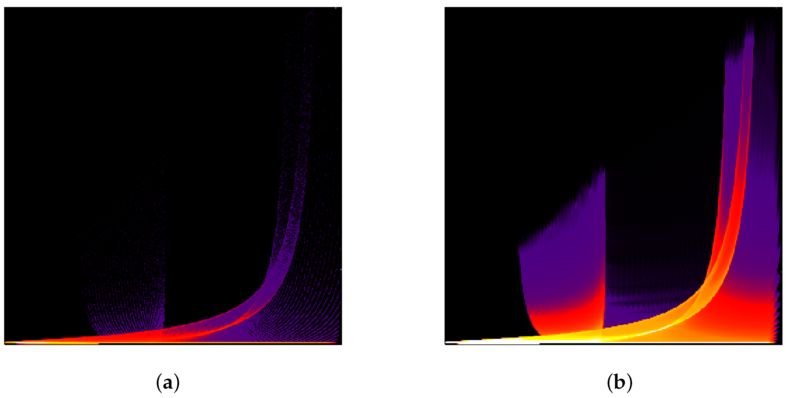
Finally, we demonstrate that scatterplots of upsampled data approach the quality of continuous scatterplots as presented by Bachthaler and Weiskopf [26] and the follow-up papers. The “tornado” dataset [32] was sampled on a uniform grid of resolution . Similar to [26], the magnitude of the velocity and the velocity in z-direction were taken as two data dimensions. In Figure 14, we show scatterplots of the original data and of the adaptively upsampled data with interpolation depth 5. The number of bins is 300 for each attribute. The quality of the upsampled scatterplot is similar to the continuous scatterplot presented in [26]. We would like to note that, rigorously speaking, evaluation of vector magnitude and interpolation are not commutative operations. Thus, the upsampling with respect to the first chosen parameter could have significant errors in both the continuous and the discrete setting. However, we intentionally followed this way to be able to compare our results with results presented in [26].
9. Discussion
9.1. Histogram Bin Size
The size of the bins of the histogram can be chosen arbitrarily. Of course, smaller bin sizes produce better results, as they can resolve better the shape of the clusters. Too large bin sizes lead to an improper merging of clusters. In terms of clustering quality, bin sizes can be chosen arbitrarily small, as very small bin sizes do not affect the clustering result negatively. However, storing a high-dimensional histogram with small bin sizes can become an issue. Our current implementation stores the histogram in main memory, which limits the bin sizes we can currently handle. This in-core solution allows us to produce decent results, as we are only storing non-empty bins. Nevertheless, for future work, it may still be desirable to implement an out-of-core version of the histogram generation. This can be achieved by splitting the histogram into parts and only storing those parts. However, an out-of-core solution would negatively affect the computation times. In addition, the smaller the bin sizes, the more upsampling is necessary.
9.2. Upsampling Rate
The upsampling rate is influenced by the local variation in the values of the multivariate field and the bin size of the histogram. Let be the bin size of the histogram. Then, an upsampling may be necessary, if two data points in attribute space are more than distance apart. As the upsampling rate is defined globally, it is determined by the largest variation within a grid cell. Let be the maximum distance in attribute space between two data points, whose corresponding points in physical space belong to one grid cell. Then, the upsampling rate shall be larger than . This ratio refers to the upsampling rate per physical dimension.
When using the adaptive scheme presented in Section 5, the upsampling rate per dimension is always a power of two. When a sufficiently high upsampling rate has been chosen, the additional computations when upsampling with the next-higher power of two in the adaptive scheme are modest, as computations for most branches of the octree have already terminated.
10. Conclusions
We present an approach for multivariate volume data visualization that is based on clustering the multi-dimensional attribute space. We overcame the curse of dimensionality by upsampling the attribute space according to the neighborhood relationship in physical space. Smooth (e.g., bi- or trilinear) interpolation was applied to the attribute vectors in a regular case to generate multidimensional histograms, where the support, i.e., all non-empty bins, is a connected component. Consequently, the histogram-based clustering did not suffer from clusters falling apart when using small bin sizes. In the presence of sharp material boundaries, natural intrinsic data discontinuities, or missing data values, the smooth interpolation scheme was locally replaced by a nearest-neighbor interpolation to avoid non-physical effects due to upsampling. We applied a hierarchical clustering method that generates a cluster tree without having to pick density thresholds manually or heuristically. In addition to a cluster tree rendering, the clustering results were visualized using coordinated views to parallel coordinates for an attribute space rendering and to physical space rendering. The coordinated views allow for a comprehensive analysis of the clustering result.
Author Contributions
Conceptualization, L.L.; Investigation, V.M.; Methodology, V.M. and L.L.; Software, V.M.; Visualization, V.M.; Writing—original draft, V.M.; and Writing—review and editing, L.L.
Funding
This work was supported in part by DFG Grants LI 1530/6-2 and MO 3050/2-1.
Conflicts of Interest
The authors declare no conflict of interest. The founding sponsors had no role in the design of the study; in the collection, analyses, or interpretation of data; in the writing of the manuscript, and in the decision to publish the results.
References
- Whalen, D.; Norman, M.L. Competition Data Set and Description. 2008 IEEE Visualization Design Contest. 2008. Available online: http://vis.computer.org/VisWeek2008/vis/contests.html (accessed on 20 June 2018).
- Competition Data Set and Description. 2010 IEEE Visualization Design Contest. 2010. Available online: http://viscontest.sdsc.edu/2010/ (accessed on 20 June 2018).
- Bellman, R.E. Dynamic Programming; Princeton University Press: Princeton, NJ, USA, 1957. [Google Scholar]
- Molchanov, V.; Linsen, L. Overcoming the Curse of Dimensionality When Clustering Multivariate Volume Data. In Proceedings of the 13th International Joint Conference on Computer Vision, Imaging and Computer Graphics Theory and Applications, Funchal, Portugal, 27–29 January 2018; SciTePress: Setubal, Portugal, 2018; Volume 3, pp. 29–39. [Google Scholar]
- Sauber, N.; Theisel, H.; Seidel, H.P. Multifield-Graphs: An Approach to Visualizing Correlations in Multifield Scalar Data. IEEE Trans. Vis. Comput. Graph. 2006, 12, 917–924. [Google Scholar] [CrossRef] [PubMed]
- Woodring, J.; Shen, H.W. Multi-variate, Time Varying, and Comparative Visualization with Contextual Cues. IEEE Trans. Vis. Comput. Graph. 2006, 12, 909–916. [Google Scholar] [CrossRef] [PubMed]
- Akiba, H.; Ma, K.L. A Tri-Space Visualization Interface for Analyzing Time-Varying Multivariate Volume Data. In Proceedings of the Eurographics/IEEE VGTC Symposium on Visualization, Norrkoping, Sweden, 23–25 May 2007; pp. 115–122. [Google Scholar]
- Blaas, J.; Botha, C.P.; Post, F.H. Interactive Visualization of Multi-Field Medical Data Using Linked Physical and Feature-Space Views. In Proceedings of the Eurographics/IEEE VGTC Symposium on Visualization (EuroVis), Norrkoping, Sweden, 23–25 May 2007; pp. 123–130. [Google Scholar]
- Daniels, J., II; Anderson, E.W.; Nonato, L.G.; Silva, C.T. Interactive Vector Field Feature Identification. IEEE Trans. Vis. Comput. Graph. 2010, 16, 1560–1568. [Google Scholar] [CrossRef] [PubMed] [Green Version]
- Maciejewski, R.; Woo, I.; Chen, W.; Ebert, D. Structuring Feature Space: A Non-Parametric Method for Volumetric Transfer Function Generation. IEEE Trans. Vis. Comput. Graph. 2009, 15, 1473–1480. [Google Scholar] [CrossRef] [PubMed]
- Linsen, L.; Long, T.V.; Rosenthal, P.; Rosswog, S. Surface extraction from multi-field particle volume data using multi-dimensional cluster visualization. IEEE Trans. Vis. Comput. Graph. 2008, 14, 1483–1490. [Google Scholar] [CrossRef] [PubMed]
- Linsen, L.; Long, T.V.; Rosenthal, P. Linking multi-dimensional feature space cluster visualization to surface extraction from multi-field volume data. IEEE Comput. Graph. Appl. 2009, 29, 85–89. [Google Scholar] [CrossRef] [PubMed]
- Dobrev, P.; Long, T.V.; Linsen, L. A Cluster Hierarchy-based Volume Rendering Approach for Interactive Visual Exploration of Multi-variate Volume Data. In Proceedings of the 16th International Workshop on Vision, Modeling and Visualization (VMV 2011), Berlin, Germany, 4–6 October 2011; Eurographics Association: Geneve, The Switzerland, 2011; pp. 137–144. [Google Scholar]
- Jain, A.K.; Dubes, R.C. Algorithms for Clustering Data; Prentice Hall: Upper Saddle River, NJ, USA, 1988. [Google Scholar]
- Han, J.; Kamber, M. Data Mining: Concepts and Techniques; Morgan Kaufmann Publishers: Burlington, MA, USA, 2006. [Google Scholar]
- Hartigan, J.A. Clustering Algorithms; Wiley: Hoboken, NJ, USA, 1975. [Google Scholar]
- Hartigan, J.A. Statistical Theory in Clustering. J. Classif. 1985, 2, 62–76. [Google Scholar] [CrossRef]
- Wong, A.; Lane, T. A kth Nearest Neighbor Clustering Procedure. J. R. Stat. Soc. Ser. B 1983, 45, 362–368. [Google Scholar]
- Ester, M.; Kriegel, H.P.; Sander, J.; Xu, X. A density-based algorithm for discovering clusters in large spatial databases with noise. In Proceedings of the Second International Conference on Knowledge Discovery and Data Mining, Portland, OR, USA, 2–4 August 1996; pp. 226–231. [Google Scholar]
- Hinneburg, A.; Keim, D. An efficient approach to clustering in large multimedia databases with noise. In Proceedings of the Fourth International Conference on Knowledge Discovery and Data Mining, New York, NY, USA, 27–31 August 1998; pp. 58–65. [Google Scholar]
- Hinneburg, A.; Keim, D.A.; Wawryniuk, M. HD-Eye: Visual Mining of High-Dimensional Data. IEEE Comput. Graph. Appl. 1999, 19, 22–31. [Google Scholar] [CrossRef]
- Ankerst, M.; Breunig, M.M.; Kriegel, H.P.; Sander, J. OPTICS: Ordering points to identify the clustering structure. In Proceedings of the 1999 ACM SIGMOD International Conference On Management of Data, Seattle, WA, USA, 1–4 June 1999; pp. 49–60. [Google Scholar]
- Stuetzle, W. Estimating the cluster tree of a density by analyzing the minimal spanning tree of a sample. J. Classif. 2003, 20, 25–47. [Google Scholar] [CrossRef]
- Stuetzle, W.; Nugent, R. A generalized single linkage method for estimating the cluster tree of a density. Tech. Rep. 2007, 19, 397–418. [Google Scholar] [CrossRef]
- Long, T.V. Visualizing High-Density Clusters in Multidimensional Data. Ph.D. Thesis, School of Engineering and Science, Jacobs University, Bremen, Germany, 2009. [Google Scholar]
- Bachthaler, S.; Weiskopf, D. Continuous Scatterplots. IEEE Trans. Vis. Comput. Graph. 2008, 14, 1428–1435. [Google Scholar] [CrossRef] [PubMed] [Green Version]
- Bachthaler, S.; Weiskopf, D. Efficient and Adaptive Rendering of 2-D Continuous Scatterplots. Comput. Graph. Forum 2009, 28, 743–750. [Google Scholar] [CrossRef] [Green Version]
- Heinrich, J.; Bachthaler, S.; Weiskopf, D. Progressive Splatting of Continuous Scatterplots and Parallel Coordinates. Comput. Graph. Forum 2011, 30, 653–662. [Google Scholar] [CrossRef] [Green Version]
- Lehmann, D.J.; Theisel, H. Discontinuities in Continuous Scatter Plots. IEEE Trans. Vis. Comput. Graph. 2010, 16, 1291–1300. [Google Scholar] [CrossRef] [PubMed]
- Lehmann, D.J.; Theisel, H. Features in Continuous Parallel Coordinates. IEEE Trans. Vis. Comput. Graph. 2011, 17, 1912–1921. [Google Scholar] [CrossRef] [PubMed] [Green Version]
- Karypis, G.; Han, E.H.; Kumar, V. Chameleon: Hierarchical Clustering Using Dynamic Modeling. Computer 1999, 32, 68–75. [Google Scholar] [CrossRef]
- Crawfis, R.; Max, N. Texture Splats for 3D Vector and Scalar Field Visualization. In Proceedings of the 4th Conference on Visualization ’93, San Jose, CA, USA, 26 October 1993; IEEE CS Press: Los Alamitos, CA, USA, 1993; pp. 261–266. [Google Scholar]
Figure 1.
Grid partition of two-dimensional dataset: The space is divided into equally-sized bins in the first dimension (a); and the non-empty bins are further subdivided in the second dimensions (b).
Figure 1.
Grid partition of two-dimensional dataset: The space is divided into equally-sized bins in the first dimension (a); and the non-empty bins are further subdivided in the second dimensions (b).

Figure 2.
(a) Grid partition of two-dimensional dataset with six different density levels; and (b) respective density cluster tree with four modes shown as leaves of the tree.
Figure 2.
(a) Grid partition of two-dimensional dataset with six different density levels; and (b) respective density cluster tree with four modes shown as leaves of the tree.

Figure 3.
Clustering of arbitrarily shaped clusters: (a) original dataset; and (b) histogram-based clustering result.
Figure 3.
Clustering of arbitrarily shaped clusters: (a) original dataset; and (b) histogram-based clustering result.

Figure 4.
Visualization of cluster hierarchy in optimized 2D star coordinates.

Figure 5.
Sensitivity of clustering results with respect to the bin size. The graph plots the number of mode clusters over the number of bins per dimension.
Figure 5.
Sensitivity of clustering results with respect to the bin size. The graph plots the number of mode clusters over the number of bins per dimension.

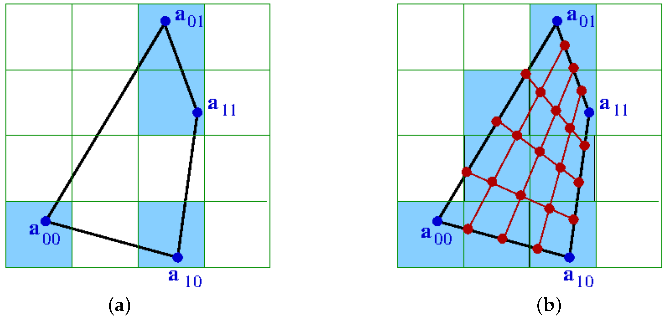
Figure 6.
Upsampling for a 2D physical space and a 2D attribute space: (a) the corner points of the 2D cell correspond to bins of the histogram that are not connected; and (b) after upsampling, the filled bins of the histogram are connected.
Figure 6.
Upsampling for a 2D physical space and a 2D attribute space: (a) the corner points of the 2D cell correspond to bins of the histogram that are not connected; and (b) after upsampling, the filled bins of the histogram are connected.

Figure 7.
(a) , tree nodes: 58; (b) , tree nodes: 39; (c) , tree nodes: 17; and (d) , tree nodes: 3. Discrete histograms with 100 bins each and cluster trees at different interpolation depth for data in Figure 9. Red bins are local minima corresponding to branching in trees. Interpolation makes histograms approach the form of continuous distribution and corrects cluster tree.

Figure 8.
Effect of bin size choice and interpolation procedure on synthetic data with known ground truth: bins are not enough to separate all clusters resulting in a degenerate tree (upper row); bins are too many to keep clusters together (middle row); and interpolation of data with the same number of bins corrects the tree (lower row). Cluster trees, parallel coordinates, and clusters in physical space are shown in the left, mid, and right columns, correspondingly.

Figure 9.
Scalar field distribution (a); and continuous histogram (b) for artificial data. Bold vertical line denotes the scaled Dirac function in the histogram.
Figure 9.
Scalar field distribution (a); and continuous histogram (b) for artificial data. Bold vertical line denotes the scaled Dirac function in the histogram.

Figure 10.
Designing a synthetic dataset: Algebraic surfaces separate clusters in physical space (a). Functions of algebraic distance to the surfaces (b) define distribution of two attributes. The resulting distribution in the attribute space in form of a 2D scatterplot (c).
Figure 10.
Designing a synthetic dataset: Algebraic surfaces separate clusters in physical space (a). Functions of algebraic distance to the surfaces (b) define distribution of two attributes. The resulting distribution in the attribute space in form of a 2D scatterplot (c).

Figure 11.
Cluster tree (upper row); parallel coordinates plot (middle row); and physical space visualization (lower row) for the 2008 IEEE Visualization Design Contest dataset, time slice 75, for original attribute space using a 10-dimensional histogram (a) before and (b) after interpolation. Several mode clusters are merged when applying our approach, which leads to a simplification of the tree and better cluster separation.

Figure 12.
Two fields of the climate simulation dataset: (a) surface temperature field is globally defined and smooth; (b) surface runoff and drainage field has non-vanishing values only for land regions and, therefore, may be discontinuous along the land–sea border; and (c) the fraction of grid cells containing a part of the land–sea border shown in red is about due to the coarse resolution of the grid.

Figure 13.
2D histograms with 25 bins each built for: (a) the original climate simulation data; (b) data upsampled using a global smooth interpolation; and (c) data upsampled using the nearest-neighbor interpolation within the cells intersecting the coastal line. The upsampling depth in (b,c) is four. Horizontal and vertical axes correspond to fields surface runoff and drainage and surface temperature.

Figure 14.
Scatterplots of the “tornado” dataset initially sampled on regular grid: original data (a); and result of adaptive upsampling with interpolation depth 5 (b).
Figure 14.
Scatterplots of the “tornado” dataset initially sampled on regular grid: original data (a); and result of adaptive upsampling with interpolation depth 5 (b).


Table 1.
Computation times for non-adaptive vs. adaptive upsampling scheme at different upsampling depths (2008 IEEE Visualization Design Contest dataset).
Table 1.
Computation times for non-adaptive vs. adaptive upsampling scheme at different upsampling depths (2008 IEEE Visualization Design Contest dataset).
| 0 | 1 | 2 | 3 | 4 | |
|---|---|---|---|---|---|
| Non-adaptive | s | s | s | 3929 s | 27,360 s |
| Adaptive | s | s | s | s | 3646 s |
| Non-empty bins | 1984 | 3949 | 6400 | 9411 | 12,861 |
| Modified adaptive | s | s | s | s | 2737 s |
| Non-empty bins | 1984 | 2075 | 2451 | 3635 | 5945 |
© 2018 by the authors. Licensee MDPI, Basel, Switzerland. This article is an open access article distributed under the terms and conditions of the Creative Commons Attribution (CC BY) license (http://creativecommons.org/licenses/by/4.0/).
Share and Cite
MDPI and ACS Style
Molchanov, V.; Linsen, L. Upsampling for Improved Multidimensional Attribute Space Clustering of Multifield Data. Information 2018, 9, 156. https://doi.org/10.3390/info9070156
AMA Style
Molchanov V, Linsen L. Upsampling for Improved Multidimensional Attribute Space Clustering of Multifield Data. Information. 2018; 9(7):156. https://doi.org/10.3390/info9070156
Chicago/Turabian StyleMolchanov, Vladimir, and Lars Linsen. 2018. "Upsampling for Improved Multidimensional Attribute Space Clustering of Multifield Data" Information 9, no. 7: 156. https://doi.org/10.3390/info9070156
Note that from the first issue of 2016, this journal uses article numbers instead of page numbers. See further details here.