Road Network Extraction from Low-Frequency Trajectories Based on a Road Structure-Aware Filter


1
Chongqing Institute of Surveying and Mapping, Ministry of Natural Resources, 10 Tengfang Ave, Chongqing 401120, China
2
School of National Defence Science and Technology, Southwest University of Science and Technology, 59 Qinglong Ave, Mianyang 621010, China
3
School of Civil Engineering and Architecture, Southwest Petroleum University, 59 Xindu Ave, Chengdu 610550, China
*
Author to whom correspondence should be addressed.
ISPRS Int. J. Geo-Inf. 2019, 8(9), 374; https://doi.org/10.3390/ijgi8090374
Submission received: 16 July 2019
/
Revised: 22 August 2019
/
Accepted: 24 August 2019
/
Published: 27 August 2019
(This article belongs to the Special Issue Algorithms and Techniques in Urban Monitoring)
Abstract
:Many studies have utilized global navigation satellite system (such as global positioning system (GPS)) trajectories in order to successfully infer road networks because such data can reveal the geometry and development of a road network, can be obtained in a timely manner, and updated on a low budget. Unfortunately, existing studies for inferring road networks from vehicle traces suffer from low accuracy, especially in dense urban regions and locations with complex structures, such as roundabouts, overpasses, and complex intersections. This study presents a novel two-stage approach for inferring road networks from trajectory points and capturing road geometry with better accuracy. First, a lane structure-aware filter is proposed to cluster vehicle trajectories influenced by high noise and outliers in order to reveal the continuous structure points of lane curves from massive trajectory points. Second, a road tracing operator is utilized to segment the road network geometry by inserting new vertices and segments to a vigorous vertex in the heading of the structure points that are extracted in the first step. Experimental results demonstrate the increased accuracy of the extracted roads and show that the proposed method exhibits strong robustness to noise and various sampling rates.
1. Introduction
Road networks are the foundation of location-based services (LBSs), such as autonomous driving, navigation, and real-time route planning [1]. As one of the principal parts of the intelligent transportation system (ITS), road maps are necessary for maintaining highly accurate and timely information [2]. Unfortunately, maintaining real-time information on road networks is challenging due to construction, closures, and accidents, etc. Clearly, manually creating and updating maps based on conventional ground-based survey techniques is costly and inefficient for meeting such a demand. Aerial imagery is considered the most common data source used for acquiring road networks rapidly and economically [3]. Unfortunately, frequent occlusions (clouds, trees and buildings), complicated pre-treatments and confusing classifications limit its application.
Currently, global positioning system (GPS) sensors are widely used on mobile platforms such as automobiles and smartphones to record the trajectory of their host [4]. Therefore, a large number of the latest real-time trajectories can be collected. In particular, the ubiquitous vehicle trajectory is a kind of geodynamic spatial data exhibiting the latest situation and high route coverage. These data contain rich information such as road geometry, driving behaviour, and commuting times [5]. Therefore, the study of extracting road networks based on vehicle trajectories has attracted the intense attention of scholars [6]. The large quantity of trajectory data generated by vehicles provides us with an unprecedented opportunity for interpreting the dynamics of urban areas. However, the continuous growth of spatial data has created considerable challenges in big data processing. In addition, the low precision of vehicle receiving equipment and the interference with GPS signals in urban environments causes positioning uncertainty and increases the uncertainty of knowledge mining.
Therefore, inferring the potential geometry and topology of road networks from vehicle traces can be difficult for three main reasons. First, the spatial and temporal uncertainty of the vehicle trajectory is caused by the measurement noise and low sampling rate of the vehicle’s GPS device [7]. Second, road networks are hierarchical, non-planar, and heterogeneous, so roads are built into complex road networks in space [8]. Finally, the density of trajectory points on roads with different capacities and flows varies greatly. Usually, trajectories on major roads are over-aggregated, however, the trajectories on minor roads may not be completely covered. Hence, discovering potential road network knowledge from unstructured trace collections is a difficult and ongoing topic [9], resulting from a gigantic knowledge disparity between the robust map representation and uncertain vehicle traces. However, there have been many innovative works on extracting and updating maps utilizing vehicle trajectories [6,10]. Due to the challenges mentioned above, road networks extracted by existing methods often have many defects, such as poor quality, unrealistic segments, and missed intersections.
To overcome these deficiencies, a road network inference approach is proposed in this work, and it provides a novel approach for constructing road networks from trajectory points at an unsatisfactory sampling frequency. Because the method of point clustering is adopted, even if there is a long sampling frequency interval, the path can be extracted as long as the trajectory point reaches a certain density. The remainder of this paper is organized as follows. Section 2 reviews related works on extracting road networks from vehicle trajectories. Section 3 outlines the proposed two-stage method for inferring road networks. Two experiments and comparative analyses with existing methods are presented in Section 4. Conclusions and suggestions are discussed in Section 5.
2. Related Work
In recent years, automatic map inference based on vehicle trajectory data has received extensive attention. Comparative studies for inferring road geometry from vehicle trajectory data were undertaken by [11] and [6]. According to the inference type of the existing works used, these methods can be classified into three categories: point clustering based on the local similarity of trajectory points, sub-trajectory clustering based on the path distance, and image morphology based on the trajectory point (line) density.
The point clustering-based method assumes that the input trajectories consist of a group of points clustered in spatial and semantic relationships [12]. For example, the mean-shift algorithm utilized trajectory data to move the seed points until each seed converged on the road centre [13,14]. Analogously, the k-means algorithm was also employed to cluster the trajectory points first [15,16] and produced links among cluster centres by mapping original trajectories to the road graphs. Additionally, the density-based spatial clustering of applications with a noise (DBSCAN) algorithm was utilized to infer road networks by clustering characteristic points [17,18]. Yang et al. [19] presented a novel method for acquiring road boundaries from vehicle trajectory points via Delaunay triangulation. Deng et al. [20] extracted the intersection modes and traffic rules of road networks adaptively using an improved algorithm based on the hierarchical trajectory clustering. Mariescu-Istodour et al. [21] introduced a method by first probing and splitting the intersections (junctions) where trajectory points with multiple principal directions exist, and then producing the road graphs between them.
The trajectory merging-based method mainly considers the continuous points as the road sampling time series and cluster trajectories or sub-trajectories based on the similarity of travel paths [22,23,24]. Ahmed et al. [25] presented a partial trajectory incremental technique that employed the Frechet distance to match the trajectories to create road graphs. Bierlaire et al. [26] developed a statistical map matching method that estimated the conditional probability of a trajectory with the consideration of both point coordinates and temporal information. Tang et al. [27] employed Delaunay triangulation and a weighted skeleton for incremental road map construction from low-frequency vehicle trajectories. He et al. [28] presented a road map inference method that utilizes the long-term observation of vehicle trajectories to create accurate road networks in dense urban regional and intricate intersections.
In addition to the two categories of vector methods mentioned above, the third category is image morphology-based, which converts the original trajectories into a geometric image (e.g., raster image or vector image) and next produces road centrelines from the image based on morphological thinning or skeletonization techniques [29,30,31,32,33]. For example, Biagioni et al. [11] transformed the input points to a kernel density estimation (KDE)-based discretized image and then applied multiple density thresholds to compute the road skeleton. Ozertem et al. presented a machine learning tool that consists of KDE and Gaussian mixture models (GMMs) [34] to refine the principal curves.
The point clustering methods for extracting road networks from unstructured trajectories are effective and robust with respect to the sampling frequency. However, the lack of track point spatial association information leads to inaccurate connection structures in the output. The trajectory merging-based methods contribute local connectivity information into map inference; however, trajectory and sub-trajectory merging require high-frequency acquisition and few outliers to work properly because the low-trajectory sampling frequency produces trajectory segments that are too long. Vector-to-grid conversion based on image morphology suffers from a loss of precision; namely, the larger the grid size is, the greater the loss of precision. At the same time, the KDE methods ignore the connectivity between GPS observations and fail to create bidirectional road networks.
In this work, we propose a novel approach to infer road network feature points by using lane structure-aware filtering based on the improved mean-shift algorithm from trajectory points, and extracting the geometric representation of each road segment by tracking local linearly distributed feature points. The primary contributions of the proposed method are summarized as follows. First, the lane structure-aware filtering method combines a dynamic radius solution and linear distribution estimation for each iteration, sifts out the continuous structural feature points of the road lane from the scattered trajectory points. Then, the structure-aware filtering method, with applications in extracting the feature structure from vehicle trajectory points in this work, and also can be used for the applications in clustering and dimensionality reduction of vehicle trajectories. Next, the novel tracing criteria is based on the similarity of seed points that guide accurate road tracing where roads are ambiguous due to overlapping or adjacency with similar headings. Finally, the proposed method is mainly point-based and robust to the sampling frequency and outliers.
3. Proposed Method
The basic observation is that even if each a trajectory exhibits sparse sampling, a map inference approach for trajectory data should also consider that a road can be traversed by a certain number of vehicles over a period of time; hence, vehicle trajectories should usually be dense. The trajectory points on different lanes often overlap each other as a result of low positioning accuracy, but the density centres are still in their lanes. In this work, filtering trajectories based on the road structure-aware method from multiple trajectory points in a local neighbourhood can not only remove the effects of extreme noise and outliers, which are unrelated to the road of interest because of low positioning accuracy, but also sift the structural feature points of road lanes by urging the trajectory points to move along the direction of the local high density of their lanes. The road lane segmentation method selects an initial vertex from the candidate queue and expands the current road segment from the initial vertex by implementing two key procedures—inserting new vertices in the direction of the active vertex to extend the road network (tracing) and connecting the current active vertex with an existing segment vertex that has already been explored when two road lanes join with same heading (connecting).
3.1. Lane Structure-Aware Filtering
The point clustering method has been widely applied to map inference because it is less susceptible to factors derived from sampling frequency. A high density of trajectory points indicates a high possibility that a road centreline exists, whereas a low density suggests that vehicles separate from the road centreline. In addition, driving heading is one of the most important movement characteristics for vehicle trajectory data and one of the principal bases for analysing the characteristics of traffic driving behaviour. Therefore, the direction-based density clustering method not only helps to reveal the clustering characteristics of the distribution of trajectory data but also helps to extract the behavioural characteristics of urban traffic flow from the vehicle traces. Therefore, a clustering approach based on lane structure-aware filtering is proposed in this work, where both the spatial distance and direction characteristics are considered in the calculation of the neighbourhood trajectory data.
3.1.1. Mean-Shift
The mean-shift algorithm, originally created by Fukunaga and Hostetler [35], is a non-parametric feature-space analysis technique for locating the maxima of a density function, and mainly applied in domains that include pattern recognition, point cloud denoising and image processing. In our previous work, the mean shift with a penalty was utilized to extract the centreline of the road network [36].
where the first item of formula (1) represents the original mean-shift algorithm and the second item penalizes the point distributed in a local centre; balances constants between the two items; is the initial coordinate (composed of x and y coordinates) for each iteration, and is the shifted coordinate after each iteration with a set neighbourhood radius R. and are the original trajectory points and seed points around the centre of for each iteration. ; used as a smooth kernel weight for rapidly decaying with a support cell radius R, where represents the Euclidean distance between two points.
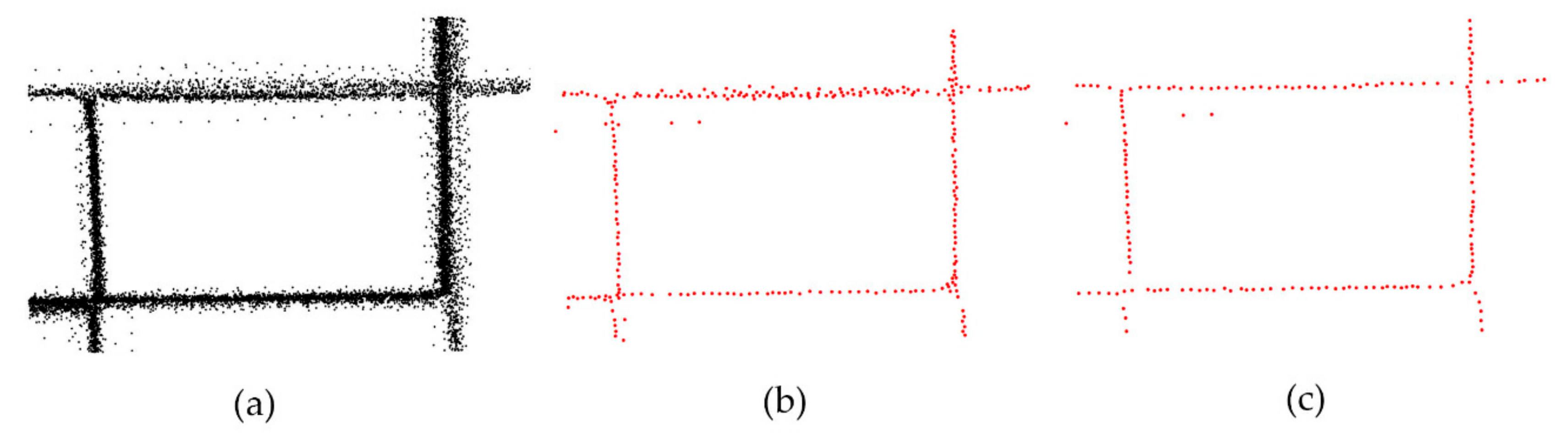
However, because the direction the vehicle is driving is not considered during neighbourhood construction, as shown in Figure 1, the mean-shift procedure fails to extract roads in detail. In this work, the heading directions are considered in the neighbourhood calculation process, and a fairly liberal heading threshold is adopted, e.g., 45°. Hence, a point is regarded as motion direction compatible if its heading follows the heading threshold of the centre point.
3.1.2. Implementation Details of Lane Structure-Aware Filtering
Using only the mean-shift algorithm constraint by the track point heading direction will fail to distinguish the structure points of the road lane from the noisy trajectory points. The largest difference compared to our previous work is that we combine a dynamic radius and linearity estimation at each iteration. The following four implementation details in the process of lane structure-aware filtering were emphasized.
- First, the distribution of the track points in different regions is not uniform. To infer roads in the sparse density region, we select all the input trajectory points as initial seeds, which is different from the existing clustering methods that use fixed equal-length sampling [15,16] or fixed gridded sampling [14].
- Second, we also need to update the heading direction of each seed while updating its location during each iteration. Instead of using the mean of the nearby original trajectory point directions, we estimate a new direction for each centre seed using the heading direction median for the original points.
- Then, since each road graph in the real world has a different width attribute, we filter the trajectory points based on a radius representing the width of the road lane. Instead of using a fixed radius for each iteration, we initiate with a small radius and enlarge the radius during the iteration process. After each iteration, we also estimate a linear distribution characteristics of each seed (detailed in Section 3.2). When a seed is linearly distributed on the lane, the next iteration will not update its location and heading. Thus, the initial radius of all seed points is set to a fixed initial value, e.g., four metres, and the radius of each iteration is increased by 0.5 metres. This dynamic radius solution, combined with linear distribution estimation, allows the lane structure-aware filter to remain effective in exploring more specialized lanes, such as ramps.
- Finally, to accelerate the contraction of the seed points to road centrelines, and to abstract the structure of roads using as few feature points as possible, the two points are substituted for one point with a mean of their positions as soon as their distance is less than one metre. Therefore, the number of seeds decreases gradually with the iteration calculation, and only a few seeds remain that are eventually located in the local intermediate position of the road lanes. These remaining points are called geometric structural points, which represent the geometric structure of the centreline of the road lanes.
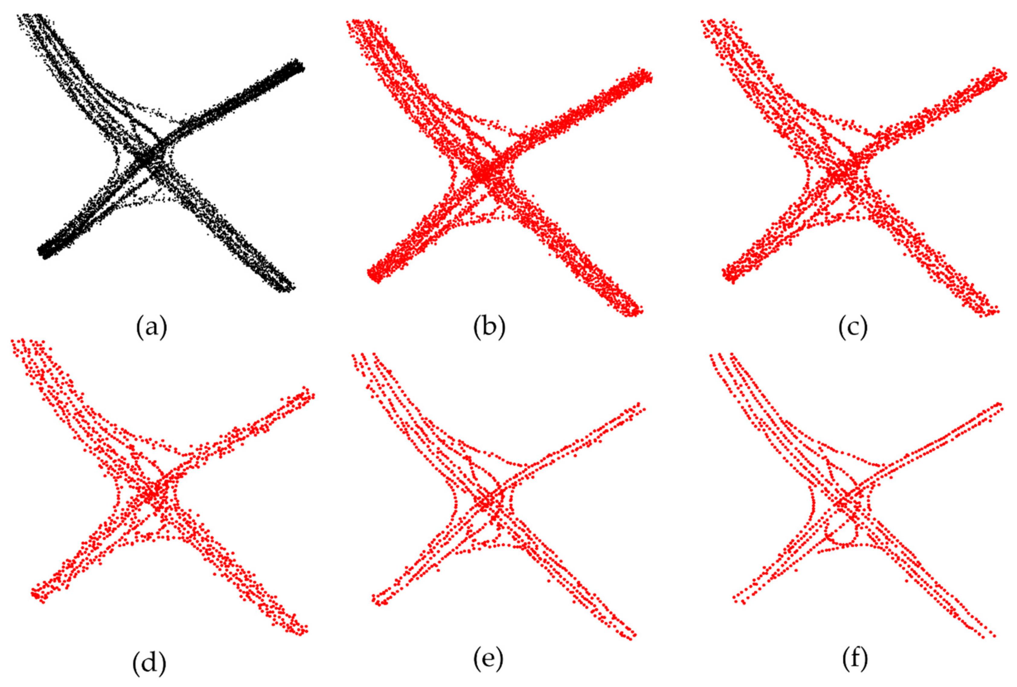
In Figure 2, we partially visualize an example of how the lane structure-aware filtering works at various iterations. The filtering operation utilizes the trajectory points to gradually sift the seed points, including shifting points towards high-density areas and merging where two points are close together. As the iterations progress, the sampling points gradually approach and fix to the lane centreline, and the number of points decreases accordingly. As illustrated in Figure 2f, the structure-aware filtering method can effectively sift out the geometric structure points of the road lane from the scattered trajectory points because the structure-aware filtering method fixes the structure points that are linearly arranged on the road segments at each iteration.
3.2. Linearity Estimation and Removing Outliers
Instead of designing an arbitrary curve, roads are usually designed to be as gradual as possible to avoid sharp turns. Even if the road is smoothly curved, it can still be considered a straight line in a local range. Recall the implementation details of the lane structure-aware filter in Section 3.1.2. We update the position and heading of seeds based on a linear distribution attribute. Principal component analysis (PCA) considers that the orientations with the largest variances are the most “important” (i.e., the most principal) [37]. Therefore, the basic concept is to evaluate the principal component of the local road lane at vertex from the seeds and utilize that as the linear distribution attribute. Thus, we adopt the classic weighted PCA to detect the lane geometric feature points that form a linear distribution with the near multipoint seed points.
At each seed point (a row vector composed of x and y coordinates) and the nearby seeds within its neighbourhood, compute a 2 × 2 weighted covariance matrix:
The eigenvalues and the corresponding eigenvectors of the covariance matrix are computed and define the value:
as the linear distribution attribute of with its local neighbourhood points .
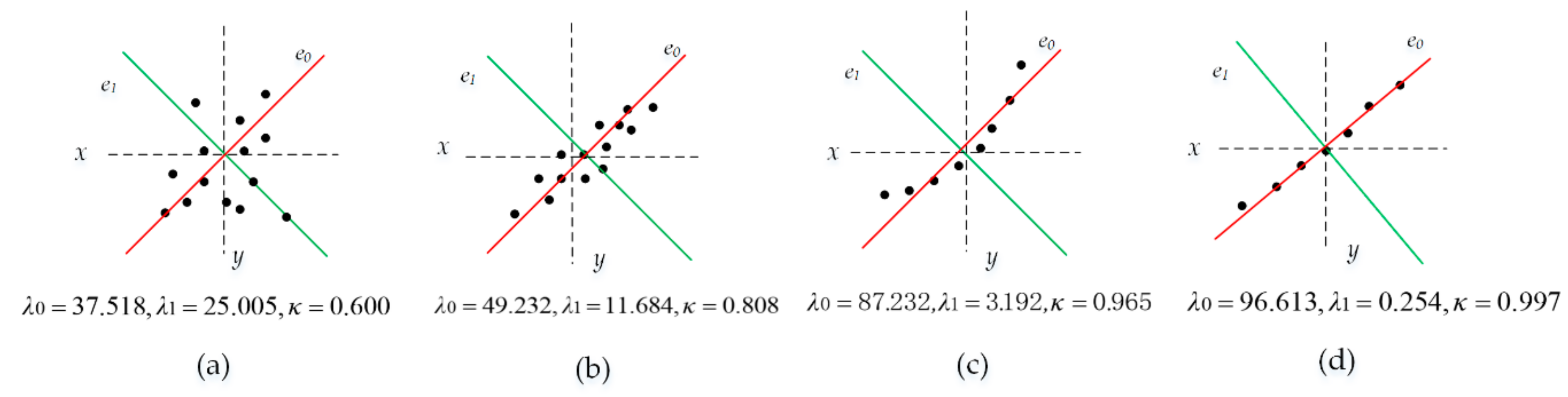
In Figure 3, the axis (red) is the first most principal direction along which the samples show the largest variation. The axis (green) is the second important direction and is orthogonal to the axis. As illustrated in Figure 3a,b, the smaller the difference between the values of and , the closer the value of is to 0.5, indicating that there is redundancy in the data. In contrast, the greater the difference of the two eigenvalues, the more the points that are distributed in the direction of the first principal component (red), as illustrated in Figure 3c,d, accordingly, the closer is to 1. Therefore, in the iterative calculation of Section 3.1.2, even if the iteration has not ended, the position and heading will not be updated when the linear distribution value of a point is greater than 0.95 because there are no redundant trajectory points around it.
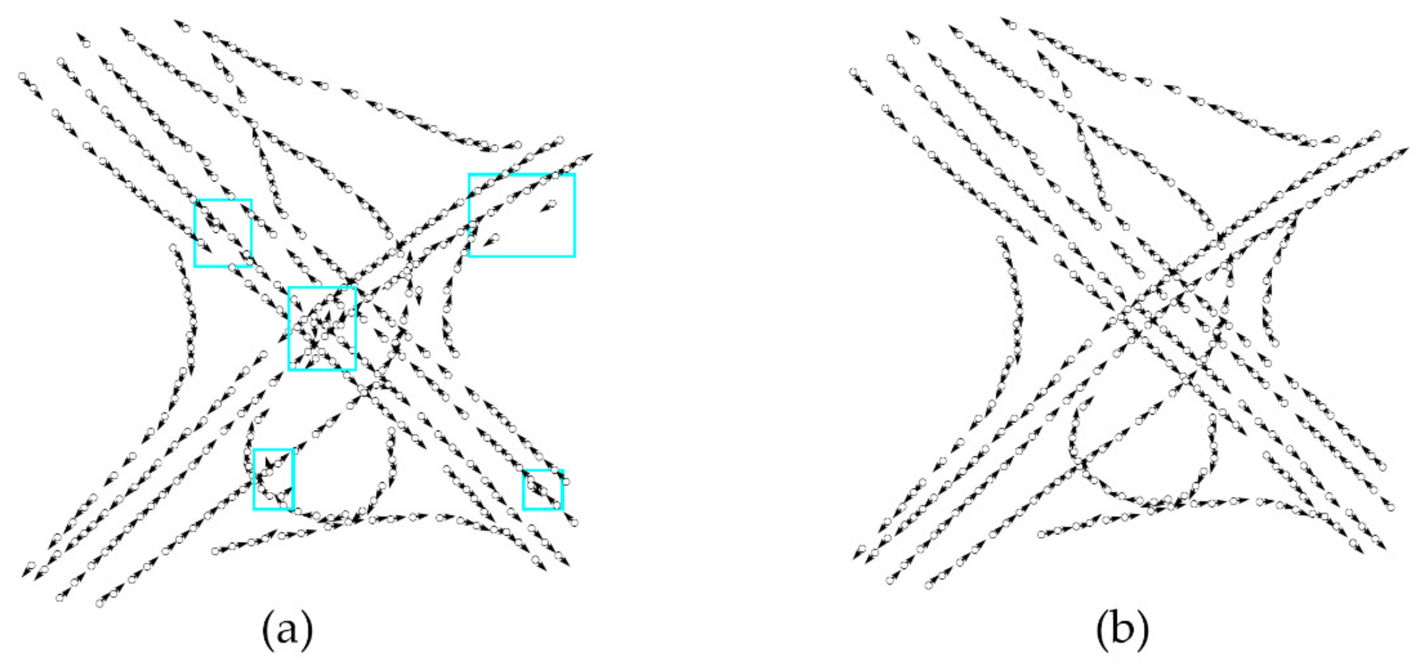
The lane structure-aware filter can capture complex geometric structural seeds of the road network with high accuracy. However, some of the identified structural seeds may be pseudo-features that should be detected and abandoned in regions that are distanced from their lanes or covered by extremely sparse trajectory points, as shown in Figure 4a, because the lane structure-aware filter aggressively filters trajectory points that do not relate to the geometry of the currently probed road during the iterative computation. This approach achieves very high precision, but unqualified trajectories become isolated points. We solve this problem by reusing the linear distribution attribute estimated at the end of the lane structure-aware filter. We select from all the structural points only the points where > 0.95 as candidate points for road tracing, as shown in Figure 4b.
3.3. Road Lane Segmentation
The road lane segmentation method gradually segments the road graph from an initial seed point by following its heading direction. The segmentation procedure uses a set of candidate points to iteratively extend the graph by inserting new vertices and segments in the direction of the active vertex and connecting when two roads with a similar heading come together. The strategy stops tracing a road lane when it arrives at a dead end, deviates from the region of interest, or connects with other roads with the same traffic direction.
3.3.1. Iterative road Lanes Tracing
The principal curve [38] technique includes an ordered set of oriented points based on local principal orientation curves [39]. In this work, the orientation explicitly derives from the seed heading. Roads are often designed to be as smooth as possible to avoid sharp turns, and major roads are straighter than minor ramps. With this prior knowledge, and the principle of the principal curve, the tracing steps iteratively along roads initialized from a seed location with the largest value from the candidate point queue, which is guided by a decision function that takes full advantage of the distance, heading and number of original trajectory points of a candidate point. Because this strategy can be guaranteed, the main roads are tracked first and then attached to the subsequently tracked ramps. Additionally, given that the road orientation may exhibit a slight discrepancy at a new vertex, the next vertex is determined from the neighbours of the active vertex based on the following conditions:
- Ensuring that the searched next vertex is close to the the search distance should be less than a set threshold.
- Ensuring that there is no sudden turn on a road lane, the orientation change .) between the two vertices of a lane should be less than the set threshold.
When the next vertex is obtained, replace with as the active vertex by tracing in the same way. This algorithm stops tracing a road lane when it arrives at a dead end, deviates from the region of interest, or connects with other road segments with a similar heading that have already been explored. In this way, tracing the road graph in an iterative pattern ensures exploiting the long-term connectivity between vehicle trajectories to accurately capture road geometry and topology as it adds each segment to the road network.
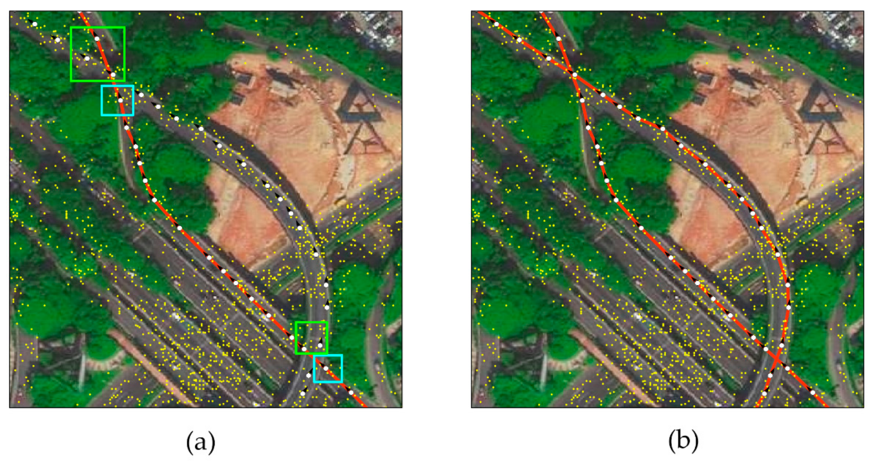
Usually, however, more than one candidate from is acquired around according to the above conditions. We found that using only the distance and heading features to determine the next vertex is not sufficient. Figure 5a shows the two ambiguous regions (highlighted rectangle) during road tracking where the road overlaps another road with a similar heading. The region in the upper left corner of Figure 5a, using only the distance and heading thresholds for extending the road, may cause the curve to track to another road. To overcome this challenge, a novel tracing criterion expressed as a scoring function is used that also considers the number of original trajectory points at the location of a structure point because the traffic flow may be slightly different at the local area of the same lane but show great differences on different lanes.
where represent the normalized features of respectively, and are calculated based on the distance, heading and density difference features of the active vertex and a candidate point . Since the range of values of each feature for varies widely, the objective function will not work well due to lack of normalization [40]. Therefore, the range of each feature should be normalized (vary between 0 and 1) on the basis of the minimum and maximum value of each feature so that it contributes approximately proportionately to the final Euclidean distance and picks the next vertex with the minimum distance. The number of original trajectory points is estimated during the lane structure-aware filter process.
3.3.2. Connecting Road Lanes
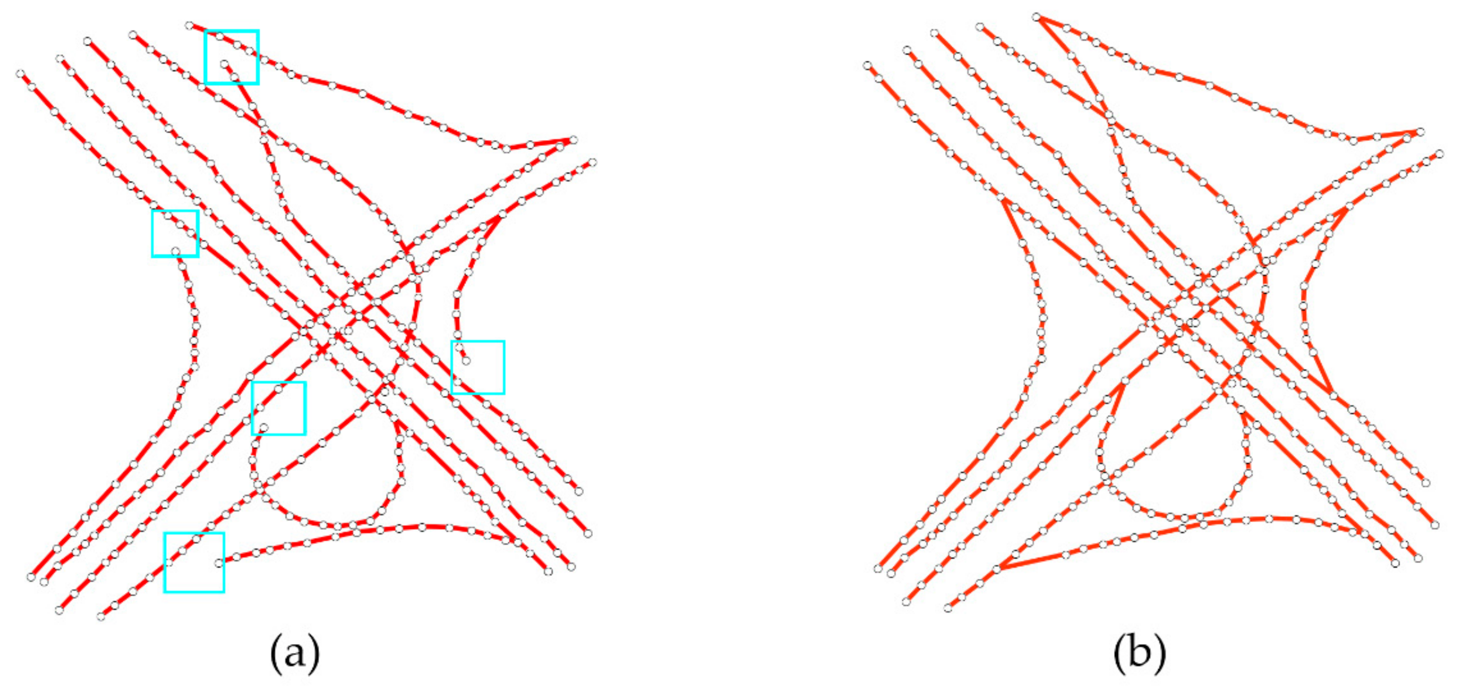
The tracing algorithm may fail to connect (trace) all road segments when the heading between two lanes is very small, as shown in Figure 6a. This often occurs on highway on-ramps and off-ramps, where the great traffic volume discrepancy between the highway and the on/off-ramp along with the small angle of the branch cause seed points on the ramp (low density) to move towards the highway (high density) during structure-aware filtering, causing the absence of one or more feature points at the confluence of the ramp, as shown in the highlighted regions in Figure 6a.
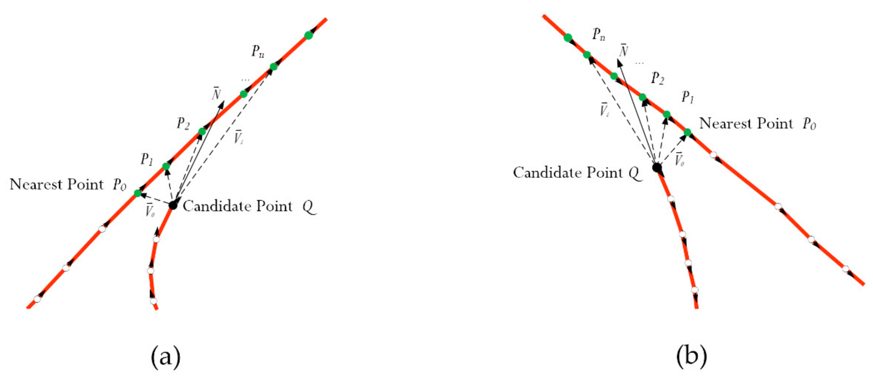
Thus, we develop a connecting procedure to correct the topological structure of the road network. First, the starting vertex or tail vertex of the dead road is chosen as the candidate vertex Q, and its extending direction vector is . As shown in Figure 7a, we search the nearest lane vertex and the following vertex on an existing road lane with the same orientation within a certain distance. For any vertex and consisting of a direction vector , we find the best point where the and vectors have the smallest angle as the connected vertex. For the case where the lane is disconnected at the starting vertex, as shown in Figure 7b, after finding the nearest vertex , the subsequent vertex is found along the opposite direction of the lane. These disconnected road segments can repair the connection in this way, as shown in Figure 6b.
4. Experiments and Discussion
To verify the effectiveness and robustness of the proposed approach, two kinds of trajectory (high-frequency sampling and low-frequency sampling) are selected to test the proposed method in this work. The basic statistics of the two trajectories are reported in Table 1, and the trajectory characteristics are summarized as follows:
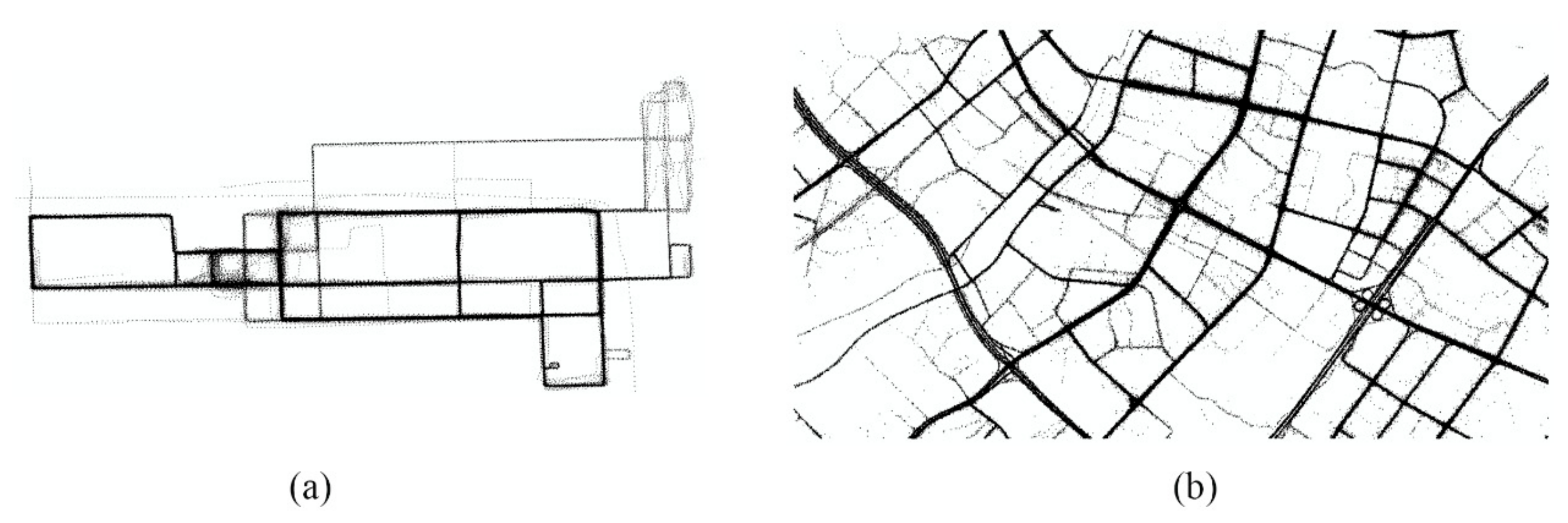
- Dongguan Taxi dataset: The Dongguan dataset was acquired by taxis from Dongguan, China [41]. The dataset covered an area of 6.04 km × 3.46 km, with approximately 2000 trajectories and 280,253 track points. This region contains complex road intersections, from diverse overpasses to small residential roads, as shown in Figure 8b.
4.1. Evaluation Method
A road network is an indispensable geographic entity and is designed as a complex network that requires higher position precision and accurate topology relationships. Three indicators introduced by Biagioni and Eriksson [11], namely, “precision”, “recall", and “F-measure”, are utilized to quantitatively evaluate the accuracy of the result of the map inference. This approach adopted a graph-sampling-based distance measure to simultaneously evaluate the geometric and topological similarities between the explored map and ground truth map. The main idea of the method is as follows.
Sampling points are sampled on each road segment equidistant from the extracted map (extracted) and the truth map (truth). The two point groups are compared utilizing a one-to-one match by a given distance threshold and counting points in each group of the matched sampling points. The accuracy of the construction map related to the truth map was quantified based on the ratio of matched sampling points, where the matched points sampling from the extracted map are represented by and the matched points sampling from the truth map are represented by . The represents the similarity of the extracted map compared with the truth map and recall represents the integrity of the extracted map compared with the truth map, where and Based on the and recall, the F-measure is computed as follows:
The value ranges from 0 to 1, with a score closer to 1 indicating that almost all the extracted roads and truth map are matched; in contrast, a score closer to 0 demonstrates very few extracted roads and ground truth are matched. Therefore, this quantitative method was utilized to measure the geometric and topologic accuracy of the extracted road network.
4.2. Quality Comparison and Discussion
According to experimental results, the neighbourhood radius for the lane structure-aware filter sets an initial fixed value of three metres and increases the radius of each iteration by 0.5 metres. The thresholds for the segment trace process are the heading of 35° and the distance of 30 metres, and the road connecting step is set at 60 metres. For comparison and evaluation, the existing road extraction methods were compared by Ahmed [6] and Kharita [42]. In previous work, we also extracted the centreline of the road network, similar to Davies [29] and Ahmed [25]. In this work, the proposed method was compared with the methods of Kharita on the same two datasets. To quantize the accuracy of the road networks inferred from the two trajectory datasets, an OpenStreetMap [43] representation of the same region was utilized as the ground truth map.
4.2.1. Visual Inspection
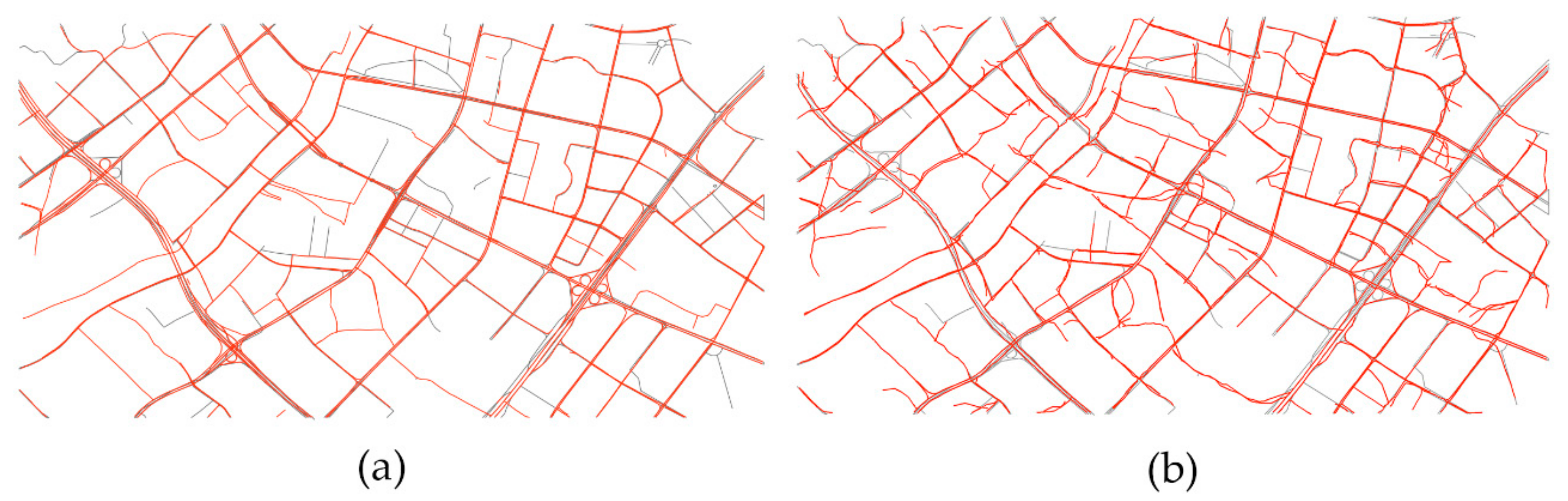
Figure 9 and Figure 10 illustrate two road network (red line) generated by the proposed method and the method by Kharita, respectively, as well as the corresponding ground truth map (grey line). One can see that that the proposed method extracted more road segments that are considered consistent with the benchmark map. Despite that Kharita’s method can also obtain a relatively complete road network from dataset 1 (high sampling frequency), it produces a few redundant edges and offset intersections from the Chicago dataset, caused by a low trajectory sampling frequency yielding trajectory segments that are too long for this technique to work properly.
4.2.2. Accuracy Results
Table 2 provides the detailed results for the length of the generated road for the two methods in different experimental regions and shows that both methods can obtain relatively complete road segments. Since Kharita’s method produces redundant segments, the total lengths of the roads extracted from the Dongguan dataset are longer.
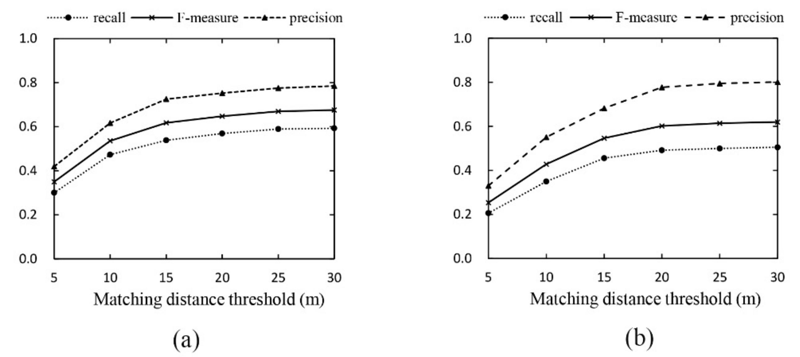
Based on the criteria proposed by Biagioni and Eriksson, the plots of the accuracies of the roads extracted from the two validation datasets are presented in Figure 11 and Figure 12. In general, the scores are greater on the Chicago dataset compared with the Dongguan dataset because the Chicago data are mostly collected by buses following regular routes; hence, the network geometry is relatively ordinary, with more trajectories covering most extracted road edges. In contrast, the Dongguan dataset is much more complex with respect to routes and intersection types and it poses a great challenge for accurate extraction.
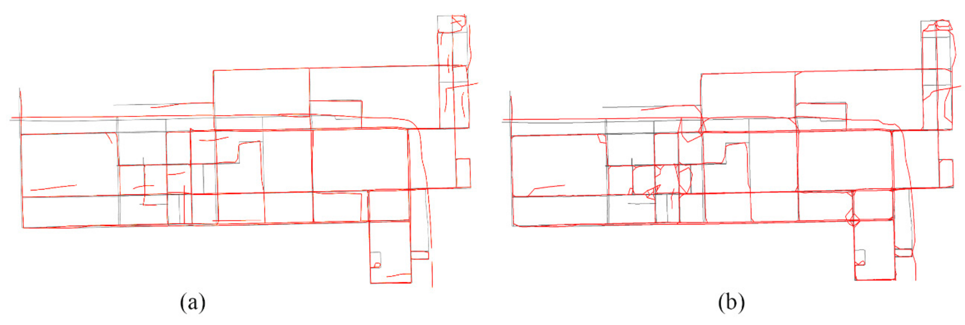
We noted that, for the high-frequency sampled Chicago dataset, the difference between the two methods’ extraction results is not obvious; however, the results differ greatly for the Dongguan dataset with low-frequency sampling trajectories. Therefore, from the perspective of the visual and quantitative evaluation, the road network extracted by the proposed method has higher effectiveness and better accuracy than the road network generated by Kharita’s method.
4.3. Discussion
Although the process presented in this work may not have achieved state-of-the-art, the results show the great capability and potential of extracting road information that is present in vehicle trajectories. First, the map inference provides a possible solution for map updates because all the missing roads form a sub-map of the complete road network, and map inference can be used to find the road skeleton of the sub-map by mining the trajectory data. Second, we focus on the road network extraction at the lane level, which is essential for high-precision, real-time maps for autonomous driving. Third, the structure-aware filtering method, with applications in dimensionality reduction and clustering of vehicle trajectory points, greatly facilitates existing dimensionality reduction and clustering techniques. Moreover, the potential information contained in the vehicle trajectory can be used to provide useful guidance and support for other emergency response purposes, such as traffic forecasting, traffic grooming, and crowd flow analysis.
As our evaluation results indicate, the proposed method was validated as an effective approach for taking low-frequency trajectory points as input to extract the road lanes, as shown in Figure 13b. However, determining how many trajectory points (lines) on a road are adequate for road network extraction is an uncertain problem. Moreover, trajectory density was influenced by self-factors, such as road grade and road structure, as well as being correlated closely with the distributed location, traffic flow, and pedestrian movement. Although this work uses the dynamic structure-aware technology to solve some problems, low-quality seeds (long distances or a heading that varies greatly) are still produced in regions of sparse trajectories that cause failures in road tracing, as shown in Figure 13a. To further deal with this limitation, additional techniques, such as trajectory interpolation, are potentially useful solutions.
5. Conclusions
The present work has demonstrated a novel two-stage approach for creating a detailed road network from vehicle trajectories that clearly advances the state-of-the art by being able to handle noisy and sparse sampling trajectories. Separating track points according to road lanes has been the greatest challenge because low-precision vehicle trajectories are scattered on the road surface. To identify potential lane branches, the structure-aware filtering method effectively sifts out the geometric structure points of the road lane from the scattered trajectory points by combining the dynamic radius and linearity estimation at each iteration. The method was validated and evaluated using two kinds of data that are sampled by high frequency and low frequency, and experimental results demonstrate better performance is achieved in geometric accuracy and topologic accuracy of the extracted road network compared with other methods. It was verified to be effective for quality improvement in low-sampling rate situations when handling the vehicle trajectory of different road structures in a feasible way.
However, the proposed method sometimes fails to infer road segments when there are not enough trajectories because the road segmentation relies on a certain density of trajectory points. Therefore, future studies will concentrate on extending the technique to work with sparse track points and improving the methodology to generate highly detailed road networks. In addition, the current approach is designed for map inference from trajectory data within given time bounds, and consequently, we plan to improve the methodology to work with map updates in streaming trajectory data.
Author Contributions
Conceptualization, Daigang Li; methodology, Daigang Li, Juntao Li; software, Daigang Li, Junhan Li; validation, Junhan Li, Juntao Li; formal analysis, Daigang Li, Junhan Li; investigation, Daigang Li; resources, Junhan Li; data curation, Juntao Li; writing—original draft preparation, Daigang Li, Junhan Li; writing—review and editing, Daigang Li, Junhan Li; supervision, Juntao Li; project administration, Daigang Li; funding acquisition, Daigang Li.
Funding
This study was funded by the Technology and Standard of National Basic Surveying and Mapping of China (2018KJ0300).
Acknowledgments
The authors would like to thank OpenITS for their initiatives in intelligent transport system. Meanwhile, we thank the editors and reviewers for their valuable comments.
Conflicts of Interest
The authors declare that they have no conflict of interest.
References
- Lu, H.C.; Tseng, V.S. Mining Cluster-Based Mobile Sequential Patterns in Location-Based Service Environments. In Proceedings of the Tenth International Conference on Mobile Data Management: Systems, Services and Middleware, Washington, DC, USA, 18–20 May 2009; pp. 273–278. [Google Scholar]
- Shi, W.; Shen, S.; Liu, Y. Automatic generation of road network map from massive GPS, vehicle trajectories. In Proceedings of the International IEEE Conference on Intelligent Transportation Systems, St. Louis, MO, USA, 4–7 October 2009; pp. 1–6. [Google Scholar]
- Das, S.; Mirnalinee, T.T.; Varghese, K. Use of Salient Features for the Design of a Multistage Framework to Extract Roads From High-Resolution Multispectral Satellite Images. IEEE Trans. Geosci. Remote Sens. 2011, 49, 3906–3931. [Google Scholar] [CrossRef]
- Bellens, R.; Vlassenroot, S.; Gautama, S. Collection and analyses of crowd travel behaviour data by using smartphones. In Proceedings of the Bivec-Gibet Transport Research Day, Namur, Belgium, 25 May 2011; pp. 536–544. [Google Scholar]
- Zheng, Y.; Li, Q.; Chen, Y.; Xie, X.; Ma, W.Y. Understanding mobility based on GPS data. In Proceedings of the International Conference on Ubiquitous Computing, Seoul, Korea, 21–24 Sepetember 2008; pp. 312–321. [Google Scholar]
- Ahmed, M.; Karagiorgou, S.; Pfoser, D.; Wenk, C. A comparison and evaluation of map construction algorithms using vehicle tracking data. Geoinformatica 2014, 19, 601–632. [Google Scholar] [CrossRef] [Green Version]
- Hoh, B.; Gruteser, M.; Xiong, H.; Alrabady, A. Preserving privacy in gps traces via uncertainty-aware path cloaking. In Proceedings of the ACM Conference on Computer and Communications Security, CCS 2007, Alexandria, VA, USA, 7 October 2007; pp. 161–171. [Google Scholar]
- Eppstein, D.; Goodrich, M.T. Studying (non-planar) road networks through an algorithmic lens. In Proceedings of the ACM Sigspatial International Symposium on Advances in Geographic Information Systems, Acm-Gis 2008, Irvine, CA, USA, 5–7 November 2008; pp. 1–10. [Google Scholar]
- Reinoso, J.F.; Ariza-López, F.J.; Barrera, D.; Gómez-Blanco, A.; Romero-Zaliz, R. A fitted B-spline method to derive a representative 3D axis from a set of multiple road traces. Geocarto Int. 2015, 31, 832–844. [Google Scholar] [CrossRef]
- Hashemi, M. A testbed for evaluating network construction algorithms from GPS traces. Comput. Environ. Urban Syst. 2017, 66, 96–109. [Google Scholar] [CrossRef]
- Biagioni, J.; Eriksson, J. Inferring Road Maps from Global Positioning System Traces. Transp. Res. Rec. J. Transp. Res. Board 2012, 2291, 61–71. [Google Scholar] [CrossRef] [Green Version]
- Li, J.; Qin, Q.; Xie, C.; Zhao, Y. Integrated use of spatial and semantic relationships for extracting road networks from floating car data. Int. J. Appl. Earth Obs. Geoinf. 2012, 19, 238–247. [Google Scholar] [CrossRef]
- Chen, C.; Lu, C.; Huang, Q.; Yang, Q.; Gunopulos, D.; Guibas, L. City-Scale Map Creation and Updating using GPS Collections. In Proceedings of the ACM SIGKDD International Conference on Knowledge Discovery and Data Mining, San Francisco, CA, USA, 13–17 August 2016; pp. 1465–1474. [Google Scholar]
- Dorum, O.H. Deriving Double-Digitized Road Network Geometry from Probe Data. In Proceedings of the 25th ACM SIGSPATIAL International Conference on Advances in Geographic Information Systems, Redondo Beach, CA, USA, 7–10 November 2017; pp. 1–10. [Google Scholar]
- Edelkamp, S.; Schrödl, S. Route Planning and Map Inference with Global Positioning Traces; Springer-Verlag New York, Inc.: New York, NY, USA, 2003; pp. 128–151. [Google Scholar]
- Stanojevic, R.; Abbar, S.; Thirumuruganathan, S.; Chawla, S.; Filali, F.; Aleimat, A. Robust Road Map Inference through Network Alignment of Trajectories. In Proceedings of the 2018 SIAM International Conference on Data Mining, San Diego, CA, USA, 3–5 May 2018; pp. 135–143. [Google Scholar]
- Wang, T.B.; Zhang, D.Q.; Zhou, X.S.; Qi, X.; Ni, H.B.; Wang, H.P.; Zhou, G. Mining Personal Frequent Routes via Road Corner Detection. IEEE Trans. Syst. Man Cybern. Syst. 2016, 46, 445–458. [Google Scholar] [CrossRef]
- Yang, B.; Zhang, Y.; Lu, F. Geometric-based approach for integrating VGI POIs and road networks. Int. J. Geogr. Inf. Sci. 2014, 28, 126–147. [Google Scholar] [CrossRef]
- Yang, W.; Ai, T.; Lu, W. A Method for Extracting Road Boundary Information from Crowdsourcing Vehicle GPS Trajectories. Sensors 2018, 18, 1261. [Google Scholar] [CrossRef] [PubMed]
- Deng, M.; Huang, J.; Zhang, Y.; Liu, H.; Tang, L.; Tang, J.; Yang, X. Generating urban road intersection models from low-frequency GPS trajectory data. Int. J. Geogr. Inf. Sci. 2018, 32, 2337–2361. [Google Scholar] [CrossRef]
- Mariescu-Istodor, R.; Fränti, P. CellNet: Inferring Road Networks from GPS Trajectories. ACM Trans. Spat. Algorithms Syst. 2018, 4, 1–22. [Google Scholar] [CrossRef]
- Wu, T.; Xiang, L.; Gong, J. Updating Road Networks by Local Renewal from GPS Trajectories. ISPRS Int. J. Geo-Inf. 2016, 5, 163. [Google Scholar] [CrossRef]
- Li, Y.; Li, Y.; Gunopulos, D.; Guibas, L. Knowledge-based trajectory completion from sparse GPS samples. In Proceedings of the ACM Sigspatial International Conference, Burlingame, CA, USA, 31 October–3 November 2016; pp. 1–10. [Google Scholar]
- Xie, X.; Bingyungwong, K.; Aghajan, H.; Veelaert, P.; Philips, W. Inferring Directed Road Networks from GPS Traces by Track Alignment. ISPRS Int. J. Geo-Inf. 2015, 4, 2446–2471. [Google Scholar] [CrossRef] [Green Version]
- Ahmed, M.; Wenk, C. Constructing street networks from GPS trajectories. In Proceedings of the European Conference on Algorithms, Ljubljana, Slovenia, 10–12 September 2012; pp. 60–71. [Google Scholar]
- Bierlaire, M.; Chen, J.; Newman, J. A probabilistic map matching method for smartphone GPS data. Transp. Res. Part C Emerg. Technol. 2013, 26, 78–98. [Google Scholar] [CrossRef]
- Tang, L.; Ren, C.; Liu, Z.; Li, Q. A Road Map Refinement Method Using Delaunay Triangulation for Big Trace Data. ISPRS Int. J. Geo-Inf. 2017, 6, 45. [Google Scholar] [CrossRef]
- He, S.; Bastani, F.; Abbar, S.; Alizadeh, M.; Balakrishnan, H.; Chawla, S.; Madden, S. RoadRunner: Improving the precision of road network inference from GPS trajectories. In Proceedings of the 26th ACM SIGSPATIAL International Conference on Advances in Geographic Information Systems, Seattle, DC, USA, 6–9 November 2018; pp. 3–12. [Google Scholar]
- Davies, J.J.; Beresford, A.R.; Hopper, A. Scalable, Distributed, Real-Time Map Generation. Pervasive Comput. IEEE 2006, 5, 47–54. [Google Scholar] [CrossRef]
- Cao, L.; Krumm, J. From GPS traces to a routable road map. In Proceedings of the Workshop on Advances in Geographic Information Systems, Seattle, DC, USA, 4–6 November 2009; pp. 3–12. [Google Scholar]
- Chen, D.; Guibas, L.J.; Hershberger, J.; Sun, J. Road network reconstruction for organizing paths. In Proceedings of the Twenty-First Annual ACM-SIAM Symposium on Discrete Algorithms, Austin, TX, USA, 17–19 January 2010; pp. 1309–1320. [Google Scholar]
- Zhang, L.; Thiemann, F.; Sester, M. Integration of GPS traces with road map. In Proceedings of the International Workshop on Computational Transportation Science, San Jose, CA, USA, 2 November 2010. [Google Scholar]
- Agamennoni, G.; Nieto, J.I.; Nebot, E.M. Robust Inference of Principal Road Paths for Intelligent Transportation Systems. IEEE Trans. Intell. Transp. Syst. 2011, 12, 298–308. [Google Scholar] [CrossRef]
- Ozertem, U.; Erdogmus, D. Locally Defined Principal Curves and Surfaces. J. Mach. Learn. Res. 2011, 12, 1249–1286. [Google Scholar]
- Fukunaga, K.; Hostetler, L. The Estimation of the Gradient of a Density Function, with Applications In Pattern Recognition; IEEE Press: Piscataway, NJ, USA, 1975; pp. 32–40. [Google Scholar]
- Li, L.; Li, D.; Xing, X.; Yang, F.; Rong, W.; Zhu, H. Extraction of Road Intersections from GPS Traces Based on the Dominant Orientations of Roads. Int. J. Geo-Inf. 2017, 6. [Google Scholar] [CrossRef]
- Kim, H.S.; Han, K.C.; Lee, K.H. Feature detection of triangular meshes based on tensor voting theory. Comput. Aided Des. 2009, 41, 47–58. [Google Scholar] [CrossRef]
- Delicado, P. Principal Curves and Principal Oriented Points. Econ. Work. Pap. 1998, 35, 197–211. [Google Scholar]
- Einbeck, J.; Tutz, G.; Evers, L. Local principal curves. Stat. Comput. 2005, 15, 301–313. [Google Scholar] [CrossRef] [Green Version]
- Aksoy, S.; Haralick, R.M. Feature normalization and likelihood-based similarity measures for image retrieval. Pattern Recognit. Lett. 2001, 22, 563–582. [Google Scholar] [CrossRef] [Green Version]
- OpenITS. Available online: http://www.openits.cn/openData2/604.jhtml (accessed on 11 May 2019).
- Stanojevic, R.; Abbar, S.; Thirumuruganathan, S.; Chawla, S.; Filali, F.; Aleimat, A. Kharita: Robust Map Inference using Graph Spanners. arXiv preprint 2017, arXiv:1702.06025. [Google Scholar]
- OpenStreetMap. Available online: http://www.openstreetmap.org/ (accessed on 11 May 2019).
Figure 1.
The process of the iterative loop and the computed results that consider only the radius of the neighbourhood in our previous work for (a) the original input trajectory points; (b) the result of five calculated iterations and (c) the result of 20 calculated iterations.
Figure 1.
The process of the iterative loop and the computed results that consider only the radius of the neighbourhood in our previous work for (a) the original input trajectory points; (b) the result of five calculated iterations and (c) the result of 20 calculated iterations.

Figure 2.
The iterative process of structure-aware filtering combined with a dynamic radius and linearity estimation; (a) the input original trajectory; (b) the result of 1 calculated iteration; (c) the result of 3 calculated iterations; (d) the result of 5 calculated iterations; (e) the result of 10 calculated iterations; (f) the result of 20 calculated iterations.

Figure 3.
Linear distribution value for different feature points. The linear distribution of point sets with different spatial distribution characteristics. The black dots represent their respective position and distribution trends on the plane. (a,b) The redundancy distribution of the two group of points; (c,d) The linear distribution of the two group of points.

Figure 4.
Removing pseudo-feature seeds and selecting candidate points based on linearity estimation. The black arrows are the driving directions of the feature points. (a) The feature points with the pseudo-feature extracted in Section 3.1; (b) The candidate points are filtered by linear distribution estimation.

Figure 5.
Ambiguous regions encountered during tracking the road segment (red) from feature seeds (white). (a) The seed inside the highlighted rectangle represents the current active vertex, and the seeds in the green rectangle represent the next vertices that satisfy the distance and heading threshold; (b) Resulting traced curves from bridging the ambiguous regions.

Figure 6.
The result of road tracing. (a) The road lanes extracted from the seed points in Figure 4b; (b) A complete overpass formed after connecting.
Figure 6.
The result of road tracing. (a) The road lanes extracted from the seed points in Figure 4b; (b) A complete overpass formed after connecting.

Figure 7.
The process of connecting road segments with similar headings. (a) Road connection strategy for roads that are disconnected at the end of the lane and connected to the vertex; (b) Road connection strategy for roads that are disconnected at the beginning of the lane and connected to the vertex.

Figure 8.
Two vehicle trajectory datasets from Chicago and Dongguan. (a) Trajectory points from Chicago; and (b) trajectory points from Dongguan.
Figure 8.
Two vehicle trajectory datasets from Chicago and Dongguan. (a) Trajectory points from Chicago; and (b) trajectory points from Dongguan.

Figure 9.
Results comparison of road networks extracted from the Chicago dataset by different methods. (a) Result generated by the proposed method; (b) result generated by Kharita’s method.
Figure 9.
Results comparison of road networks extracted from the Chicago dataset by different methods. (a) Result generated by the proposed method; (b) result generated by Kharita’s method.

Figure 10.
Results comparison of road networks extracted from the Dongguan dataset by different methods. (a) Result generated by the proposed method; (b) result generated by Kharita’s method.
Figure 10.
Results comparison of road networks extracted from the Dongguan dataset by different methods. (a) Result generated by the proposed method; (b) result generated by Kharita’s method.

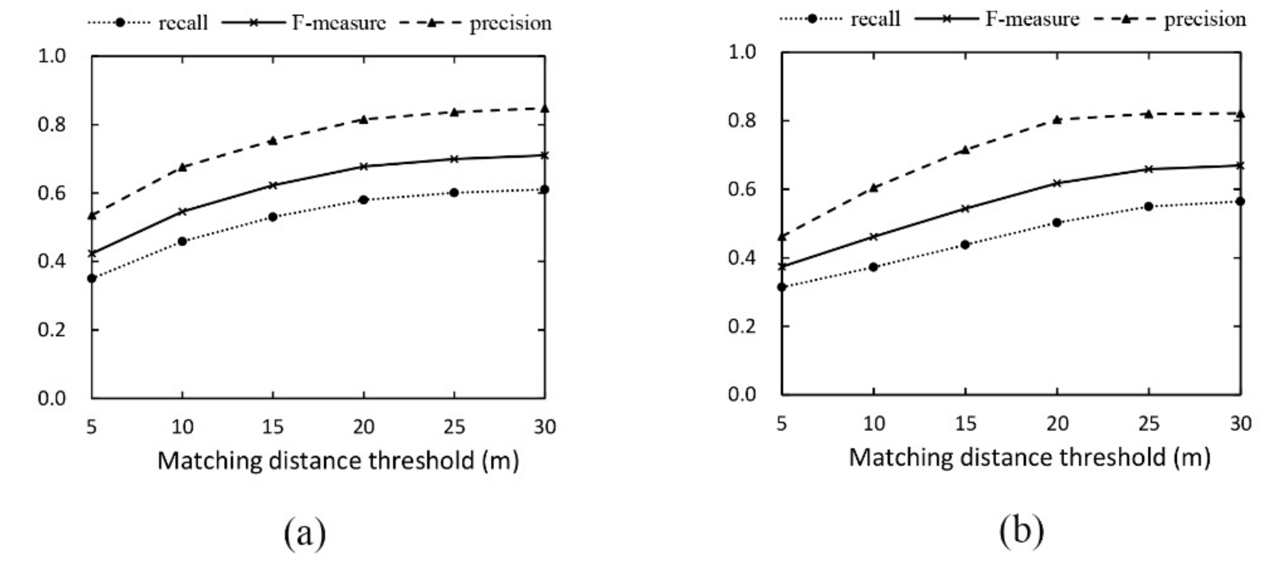
Figure 11.
Accuracy assessment of the road network extracted from Chicago. (a) Result of the proposed method; (b) Result of Kharita’s method.
Figure 11.
Accuracy assessment of the road network extracted from Chicago. (a) Result of the proposed method; (b) Result of Kharita’s method.

Figure 12.
Accuracy assessment of the road network extracted from Dongguan. (a) Result of the proposed method; (b) Result of Kharita’s method.
Figure 12.
Accuracy assessment of the road network extracted from Dongguan. (a) Result of the proposed method; (b) Result of Kharita’s method.

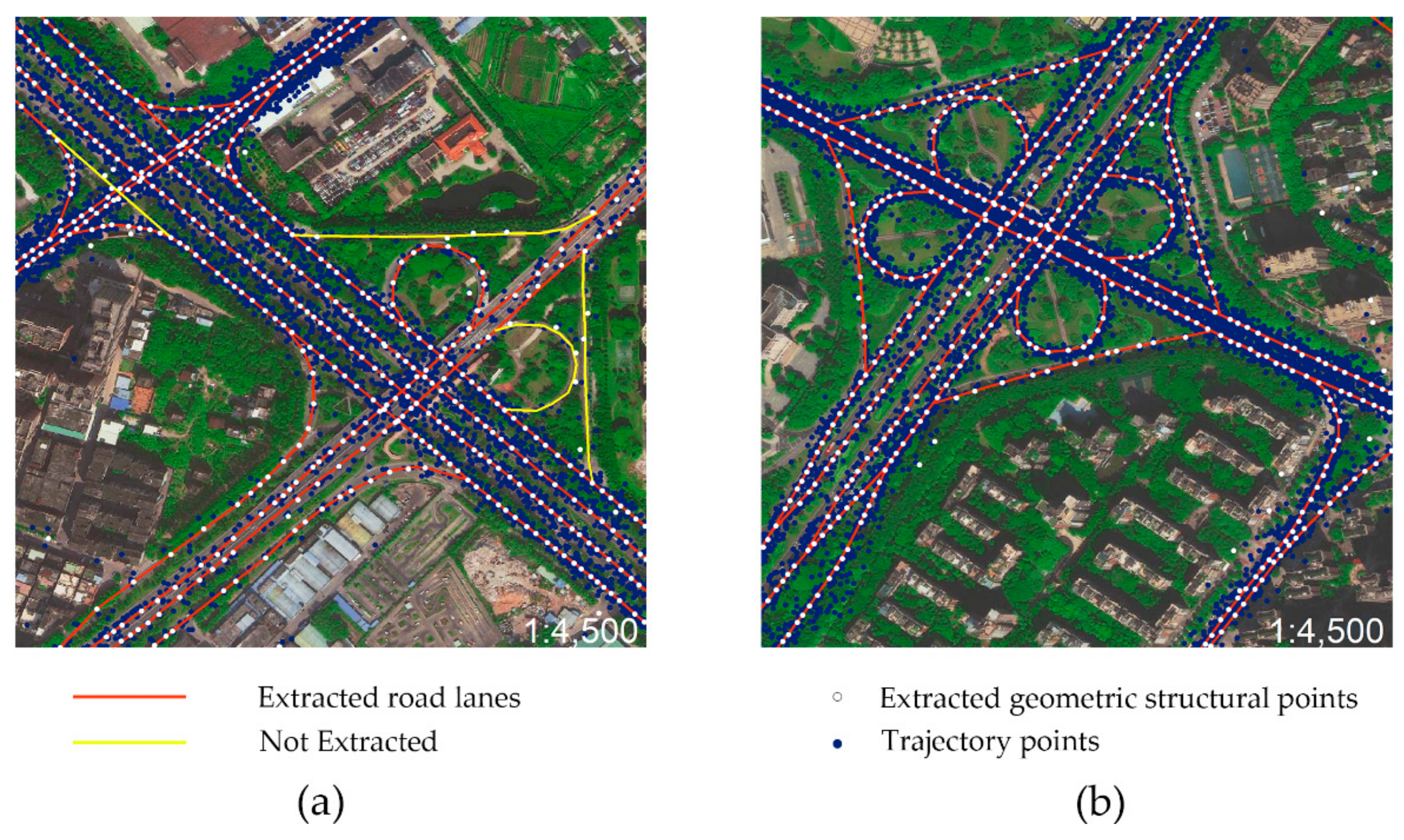
Figure 13.
Limitation of trajectory point density, indicating the proposed method fails to trace the road segments where with few trajectory points exist. (a) Few trajectory points on some lanes of the overpass; (b) trajectory points on all lanes of the overpasses have reached a certain density.
Figure 13.
Limitation of trajectory point density, indicating the proposed method fails to trace the road segments where with few trajectory points exist. (a) Few trajectory points on some lanes of the overpass; (b) trajectory points on all lanes of the overpasses have reached a certain density.


Table 1.
Comparing the features of the two datasets.
| Dataset | Trajectory Points | Average Sampling Rate (s) | Average Distance (m) |
|---|---|---|---|
| Chicago | 118,364 | 3.61 | 30.77 |
| Dongguan | 280,253 | 50.13 | 321.47 |
Table 2.
Comparing the length of the road extracted by the different methods.
| Region | Length of Generated Roads (m) | ||
|---|---|---|---|
| Truth | Proposed | Kharita | |
| Chicago | 60,009.34 | 52,711.44 (87.84%) | 49,597.22 (82.65%) |
| Dongguan | 214387.311 | 181546.577(83.57%) | 187897.199(86.49%) |
© 2019 by the authors. Licensee MDPI, Basel, Switzerland. This article is an open access article distributed under the terms and conditions of the Creative Commons Attribution (CC BY) license (http://creativecommons.org/licenses/by/4.0/).
Share and Cite
MDPI and ACS Style
Li, D.; Li, J.; Li, J. Road Network Extraction from Low-Frequency Trajectories Based on a Road Structure-Aware Filter. ISPRS Int. J. Geo-Inf. 2019, 8, 374. https://doi.org/10.3390/ijgi8090374
AMA Style
Li D, Li J, Li J. Road Network Extraction from Low-Frequency Trajectories Based on a Road Structure-Aware Filter. ISPRS International Journal of Geo-Information. 2019; 8(9):374. https://doi.org/10.3390/ijgi8090374
Chicago/Turabian StyleLi, Daigang, Junhan Li, and Juntao Li. 2019. "Road Network Extraction from Low-Frequency Trajectories Based on a Road Structure-Aware Filter" ISPRS International Journal of Geo-Information 8, no. 9: 374. https://doi.org/10.3390/ijgi8090374
Note that from the first issue of 2016, this journal uses article numbers instead of page numbers. See further details here.