Estimating Autonomous Vehicle Localization Error Using 2D Geographic Information

Abstract

Accurately and precisely knowing the location of the vehicle is a critical requirement for safe and successful autonomous driving. Recent studies suggest that error for map-based localization methods are tightly coupled with the surrounding environment. Considering this relationship, it is therefore possible to estimate localization error by quantifying the representation and layout of real-world phenomena. To date, existing work on estimating localization error have been limited to using self-collected 3D point cloud maps. This paper investigates the use of pre-existing 2D geographic information datasets as a proxy to estimate autonomous vehicle localization error. Seven map evaluation factors were defined for 2D geographic information in a vector format, and random forest regression was used to estimate localization error for five experiment paths in Shinjuku, Tokyo. In the best model, the results show that it is possible to estimate autonomous vehicle localization error with 69.8% of predictions within 2.5 cm and 87.4% within 5 cm.

1. Introduction

Accurately and precisely knowing the location of the vehicle is a critical requirement for safe and successful autonomous driving. One source of positioning information is Global Navigation Satellite Systems (GNSS). Within dense urban environments, however, the positional accuracy of solely using GNSS can exhibit errors of tens of meters due to the blockage and reflection of the satellite signal [1]. Hence, self-driving vehicles employ additional vision and range-based sensors to help determine their location. One example is the use of light detection and ranging (LiDAR) sensors which use ultraviolet, visible or near-infrared light to measure the distances to nearby objects, creating a local map of the vicinity. This local map or input scan can then be used to register against a prebuilt map to obtain a position. Despite the advancement in LiDAR sensor technology, map-based localization can still suffer from error, arising from sources such as the input scan or the choice of map matching algorithm.

The sources of localization error for map-based localization are numerous. Existing research has focused on improving the map matching algorithms [2], as well as producing increasingly accurate High Definition maps [3]. What is not yet clear is the impact of the representation of the environment within the map as a source of localization error, i.e., how does the configuration of features within the local vicinity affect localization accuracy? For example, within a tunnel or urban canyon environment, even with a locally and globally accurate map, the lack of longitudinal features in the map can cause localization error in the traveling direction.

Javanmardi et al. [4] posit that localization error is, in fact, tightly coupled with the representation of the environment in the map. For example, in areas of the map where there are numerous unique features in a distinct configuration, the accuracy of localization is high. Conversely, in areas where there is a lack of environmental objects, the quality of map matching degrades. Considering this relationship, it is therefore theoretically possible to estimate localization error at any point, by quantifying the environment in the local vicinity. This localization ‘error model’ can then be used to identify areas which may potentially have high positioning error, which in turn could allow autonomous vehicles to adapt their sensors or alert drivers of these potentially ‘hazardous’ areas. In addition, it could inform road management organizations on where to install artificial roadside objects to help improve localization.

Existing work on estimating autonomous vehicle localization error has been limited to 3D point cloud format [4,5]. There are several challenges with this approach. Firstly, localization error can only be estimated for an area if a prebuilt point cloud map is available. If not, data must be collected, which can be costly and time-consuming. These 3D point cloud maps also require substantial effort to maintain and keep up to date. Secondly, the large size of the point cloud data can make it challenging to manage. For example, a 300×300 m area may consist of over 250 million points. Coupled with the unstructured nature of the data, this leads to a large amount of pre-processing, processing, and subsequent management. Considering these challenges, there is a need to explore whether other mapping formats and sources of data, such as geographic information, can offer an alternative approach for estimating vehicle localization error.

This paper aims to estimate autonomous vehicle localization error using 2D geographic information. The main objective is to leverage 2D geographic information’s availability, wide coverage and comparatively ‘light’ data alternative for estimating localization error. This work builds upon Javanmardi et al.’s [4] format-agnostic map evaluation criteria, by defining seven new factors that are specific for 2D geographic information. The resulting work can enable the estimation of localization error without requiring the collection of data to create a prebuilt map. It can help identify and highlight areas with high localization error – either as the result of the map itself, or the real-world environment. Further, the estimated error model can be used in conjunction with other sensor information to improve the accuracy of localization [5].

The remainder of this paper is structured as follows: in Section 2, a short overview of autonomous vehicles and vehicle localization is presented. Section 3 presents an overview of geographic information and the different datasets available. Related works are presented in Section 4. Section 5 describes the formulation of the seven map evaluation factors. The method and results are presented in Section 6 and Section 7 respectively. Following a discussion on the capability of 2D geographic information for estimating vehicle localization error, and the advantages and challenges of the approach, the final Section presents the conclusions.

2. Autonomous Vehicles

Self-driving cars (also known as driverless or autonomous cars) are ground vehicles capable of sensing their environments and navigating without human input. There are two crucial components to successful autonomous driving: 1) Vehicle self-localization (knowing where the vehicle is), and; 2) Motion planning (how to move the vehicle safely).

2.1. Vehicle Localization

Localization is the estimation of where a vehicle is situated in the world. While Global Navigation Satellite Systems can provide a position with meter-level accuracy, this is insufficient for the application of autonomous driving. One meter can be the difference between driving safely on the road in the correct lane and driving along the pavement. Centimeter-level positional accuracy is therefore required for successful autonomous driving. To achieve this, autonomous vehicles are equipped with a myriad of sensors, including LiDAR, radar, and onboard cameras.

Currently, research is focused on two main approaches for localization: 1) camera-based, and; 2) LiDAR-based. Camera-based systems use images from a single camera or multiple cameras to determine the change in position over time relative to a starting position. Cameras are low-cost, lightweight and offer high resolution. However, as they utilize visible and ambient light, they are greatly affected by illumination changes and weather conditions. In contrast, LiDAR-based systems use emitted light and are therefore far less affected by environmental conditions. Compared to cameras, LiDAR sensors are more expensive, heavier and have a much lower resolution. Despite this, recent developments in miniaturization and density enhancements have resulted in smaller LiDAR sensors with higher resolution. Additionally, increased competition between sensor manufacturers has drastically reduced prices, therefore increasing the popularity of LiDAR-based systems.

LiDAR-based approaches can be broadly split into two categories: simultaneous localization and mapping (SLAM), and map matching. For SLAM-based approaches, mapping and localization are conducted concurrently. As the map is built, the displacement of the vehicle is calculated over time to obtain a position. While it works well over short distances, SLAM suffers from accumulative error over long distances. For map matching approaches, a map is prebuilt using a high-end mobile mapping system. Subsequently, the LiDAR scan from an autonomous vehicle can then be used to match against the prebuilt map to obtain a position. Despite the importance of accurate vehicle self-localization, there is yet to be an international standard for required accuracy. As guidance, ISO 17572 recommend a positional accuracy of 25 cm or less for location referencing [6,7]. Similarly, the Japanese government’s Cross-ministerial Strategic Innovation Promotion (SIP) Program also recommends a mapping accuracy of 25 cm based on satellite image resolution and the physical width of a car tire.

2.2. Sources of Localization Error for LiDAR Map Matching

Sources of localization error for map matching using LiDAR can be divided broadly into four categories: 1) Input scan; 2) Matching algorithm; 3) Dynamic phenomena, and; 4) Prebuilt map.

Firstly, errors from the input scan may be dictated by choice of the laser scanner. For example, the lower-end Velodyne VLP-16 has 16 laser transmitting and receiving sensors with a range of up to 100 m. In contrast, the latest model (VLS-128) has 128 sensors and a range of up to 300 m, allowing the capture of more detail in a wider area, thus enabling more accurate map matching. In addition, distortion can be introduced during the capture phase when in motion—a vehicle traveling at 20 m/s, with a scanner at 10Hz would result in a 2 m distortion as the scanner rotates 360 degrees. Errors can also be introduced in the post-processing where the input scan is required to be downsampled for the matching algorithm. While this reduces noise within the data, it can also remove features and details that are useful for map matching.

Secondly, the choice of the matching algorithm can be a source of error. As matching is an optimization problem, some algorithms are designed to be more robust to local optimum, while others are more immune to initialization error [8]. For example, Normal Distribution Transform (NDT) [9,10] is more resilient to sensor noise and sampling resolution than point-to-point based Iterative Closest Point (ICP) matching algorithms, but suffers from slower convergence speed. This is because point clouds are discretized into a set of local normal distributions (ND), at a specified grid size, during the initialization step of NDT [11]. By using ND maps rather than the point cloud directly, errors derived from slight environmental differences between the map and the input scan can be mitigated.

Thirdly, dynamic phenomena in the environment can contribute to error. During the mapping phase, if a large vehicle such as a lorry or a bus blocks the laser scanner, then a large portion of the map will be missing. During the localization phase, some phenomena or features may have moved or shifted. For example, parked cars found in the prebuilt map may have since moved or buildings may have been built or demolished. Furthermore, seasonal changes such as the presence and absence of leaves on trees between the mapping and localization phases can introduce error.

Lastly, the prebuilt map itself is a source of error. As mentioned earlier, having a highly accurate map does not always result in a low localization error. There are instances within the environment, e.g., tunnels, urban canyons, open spaces whereby map matching is not a suitable localization method. In these cases, it is the physical attributes of the phenomena and their representation on the map which is the source of localization error. This is discussed further in the next section.

2.3. Quantifying the Sources of Map-derived Errors

To quantify the sources of map-derived errors, Javanmardi et al. [3] defined four criteria to evaluate a map’s capability for vehicle localization: 1) feature sufficiency; 2) layout; 3) local similarity, and; 4) representation quality.

Feature sufficiency describes the number of mapped phenomena in the vicinity which can be used for localization. For example, within urban areas, buildings and other built structures provide lots of features to match against, resulting in more accurate localization. An insufficient number of features in the vicinity (such as found in open rural areas) may result in lower localization accuracy.

The layout is also an important consideration, as it is not simply the number of features in the vicinity, but also how they are arranged. Even if there are lots of high-quality features nearby, if they are all concentrated in one direction, the quality of the matching degrades.

To further compound the issue, in certain scenarios, even with sufficient and well-distributed features, accurate localization remains difficult due to local similarity. In these cases, there may be geometrically similar features either side of the vehicle, making it difficult during the optimization process to determine the position in the traveling direction.

Lastly, representation quality describes how well a map feature represents its real-world counterpart. In theory, the closer the map is to reality, the more accurate the prediction. It is important to note, however, that this criterion is slightly different from the level of abstraction or generalization of the map. For example, a flat wall can be highly abstracted as a single line but still have high representation quality.

3. Geographic Information (GI)

Geographic information represents real-world phenomena implicitly or explicitly associated with a location relative to the Earth [12]. It can allow users to visualize, interrogate and query spatial relations between multiple datasets through layering. Objects and phenomena can be abstracted into points, lines, or polygons (vector) or cells (raster) [13]. Sources of geographic information can range from authoritative sources such as national mapping agencies, to open sources such as OpenStreetMap. The different sources of GI data will be discussed in more detail below in Section 3.1 and Section 3.2.

From local to regional to international, geographic information is designed to address spatial problems at specific scales [14]. The scale is important because different processes occur at different levels [15]. For example, when examining forest cover in Asia, it may not be appropriate to consider every single tree as an individual feature. Scale, in turn, is closely related to the accuracy, precision, and generalization of geographic information. With geographic information, the producer of the data has to decide on how much detail should be displayed and how the data should be generalized for the specific application [14]. Due to its abstracted nature, geographic information may therefore not have the necessary spatial resolution to address building or feature level problems, such as indoor ventilation or facilities management.

3.1. Geospatial Information Authority of Japan

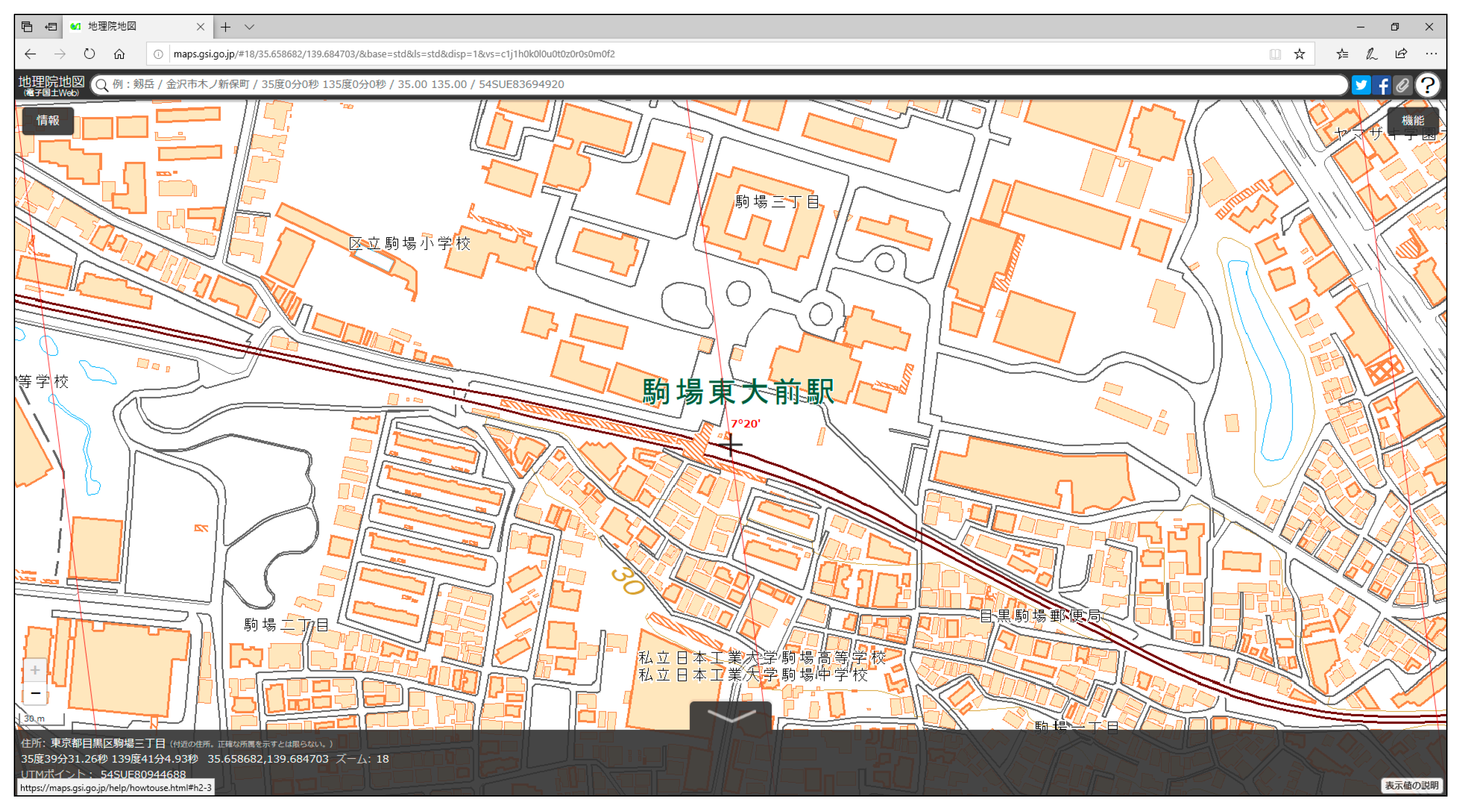
The Geospatial Information Authority of Japan (GSI – previously known as the Geographical Survey Institute) is the national mapping agency of Japan. The organization conducts surveys across the country with the aid of GPS-based control stations. Using the collected data, various thematic maps (land use, land condition, active faults) are produced for purposes such as disaster prevention and national development. In addition, GSI produces a series of topographic maps at multiple scales (1:25,000 to 1:5,000,000) covering the whole country. Specifically, the 1:25,000 map includes 13 layers including administrative boundaries, building footprints, and road edge. The data is freely available for download from an online portal (https://fgd.gsi.go.jp/download/menu.php) in GML format. Figure 1 shows an example of the 1:25,000 topographic base map.

3.2. OpenStreetMap

First introduced in 2004, OpenStreetMap is an open source collaborative project providing user-generated street maps of the world. As of March 2019, the project has over 5.2 million contributors to the project who create and edit map data using GPS traces, local knowledge, and aerial imagery. In the past, commercial and governmental mapping organizations have also donated data towards the project.

Features added to OSM are modeled and stored as tagged geometric primitives (points, lines, and polygons). For example, a road may be represented as a line vector geometry with tags such as ‘highway = primary; name:en = Ome Kaido; oneway = yes’. Despite OSM operating on a free-tagging system (and thus allowing a theoretically unlimited number of attributes and tag combinations), there is a set of commonly used tags for primary features which operate as an ‘informal standard’ [16].

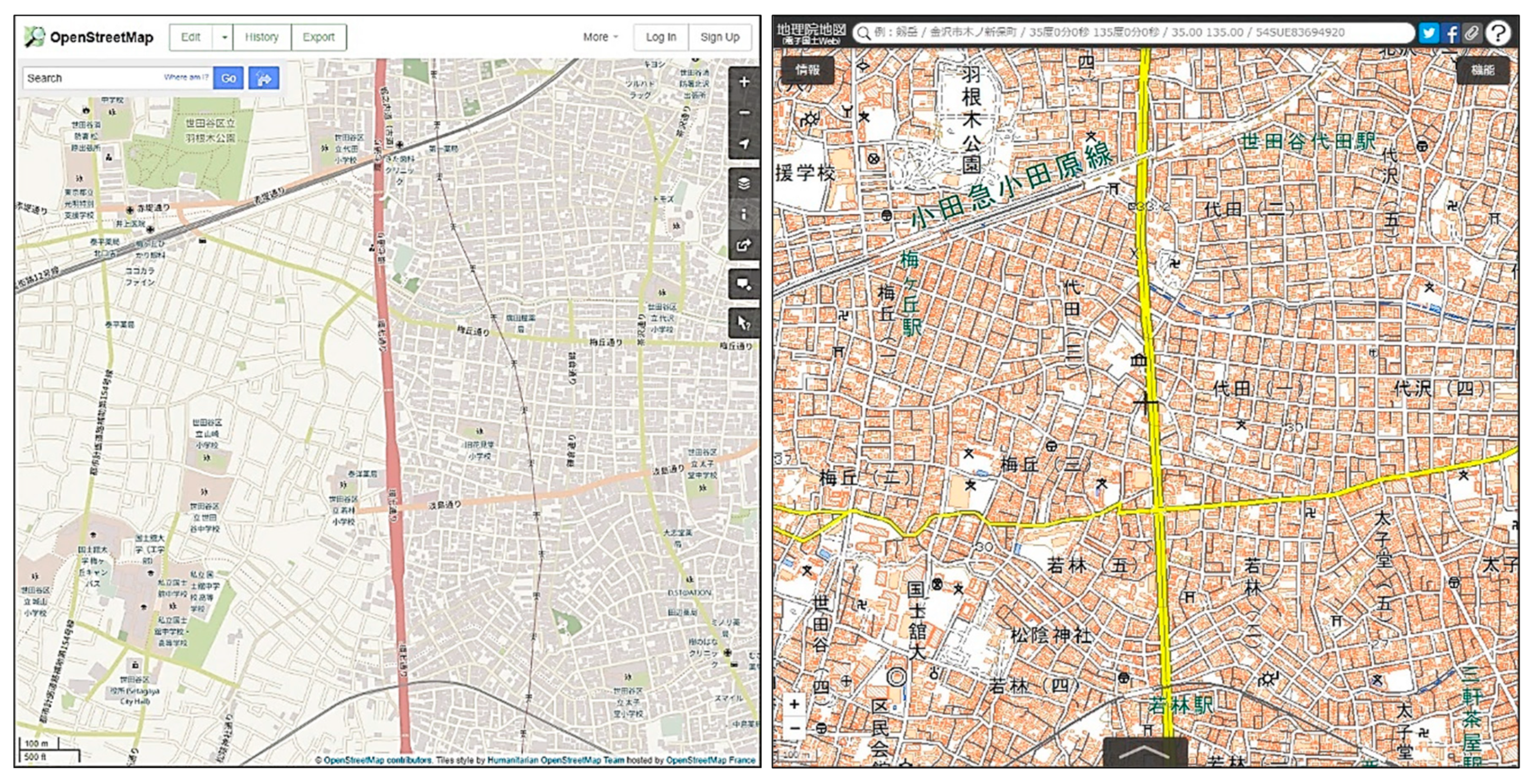
As with any user-generated content, OSM attracts concerns about data quality and credibility. Figure 2 shows a comparison between OSM and data from the Geospatial Information Authority of Japan. Extensive research has been conducted on assessing the quality of OSM datasets, including evaluating the completeness of the data. For example, Barrington-Leigh and Millard-Ball [17] estimate the global OSM street layer to be ∼83% complete, with more than 40% of countries having fully mapped networks. When comparing the number of OSM tags in Japan to official government counts (

Table 1. Coverage of OSM tags in Japan 2017 [18].

Tag	Count (Actual)	Count (OSM)	Coverage
School	36,024	45,568	126.5% 1
Fire department	5604	5028	89.7%
Police station	15,034	13,152	87.5%
Post office	24,052	20,795	86.5%
Traffic lights	191,770	108,498	56.6%
Convenience store	55,176	30,710	55.7%
Bank	13,595	7077	52.1%
Gas station	32,333	8944	27.7%
Pharmacy	58,326	7842	13.4%
Shrine	88,281	10,292	11.7%
Temple	85,045	9610	11.3%
Post box	181,523	7522	4.1%
Vending machine	3,648,600	10,311	0.3%

¹ Within OSM, there are many instances where multiple nodes and areas represent the same school (primary and secondary). This results in an overcount, and a coverage rate of higher than 100%.

), ‘completeness’ varies with different features [18]. While fire departments, police stations and post offices are well represented, temples and shrines are underrepresented. Despite this variance in completeness, OSM still represents a viable and useful source of geospatial data. In fact, in certain areas, OSM is more complete and more accurate (for both location and semantic information) than corresponding proprietary datasets [19,20]. As mapping data are abstract representations of the world, it can also be argued that a map can never truly be complete. Instead, mapping data should be collected as fit-for-purpose, and specific for the required application. OSM has been successfully used in a wide variety of practical and scientific applications from different domains [21,22,23], demonstrating the usefulness of crowdsourced mapping data.

4. Related Work

Within the field of autonomous vehicles, geographic information is used in a number of ways, from routing to localization to pose correction. Hentschel and Wagner [24] proposed the use of geometric and semantic information from OpenStreetMap for the localization, path planning and control of an autonomous robot. Building footprints were used in conjunction with 2D laser scans to localize the robot. Senlet et al. [25] combined satellite and road maps from Google Static Maps API with stereo visual odometry for global vehicle localization. Stereo depth maps were used to reconstruct the scene and compared with the 2D maps to obtain a position. Floros et al. [26] uses OpenStreetMap data with visual odometry for vehicle global localization. Specifically, mapping was used to compensate for the drift that visual odometry accumulates over time, thus improving localization quality. Similarly, Vysotska and Stachniss [27] incorporates building information from OpenStreetMap to correct the robot’s pose using graph-based SLAM.

For the estimation of localization error derived from the environment and map, Javanmardi et al. [4] proposed ten map evaluation factors to quantify the capability of normal distribution (ND) maps for vehicle self-localization. The results show that mean error can be modeled with RMSE and R² of 0.52 m and 0.788 respectively. The subsequent error model was then used to dynamically determine the NDT map resolution, resulting in a reduction of map size by 32.4% while keeping mean error within 0.141 m. Akai et al. [5] estimate the error of 3D NDT scan matching for an area beforehand in a pre-experiment. This was then used in the localization phase for pose correction. For both studies [4,5], the estimation of localization error used 3D point cloud and ND maps. As far as the authors are aware, no previous study has investigated the use of geographic information as a proxy for the estimation of autonomous vehicle localization error.

5. Map Evaluation Factors

5.1. Formulating Map Evaluation Criteria for 2D Geographic Information

Javanmardi et al.’s [4] ten map evaluation factors were used as a basis to formulate new factors for 2D geographic information. Unlike the four map evaluation criteria described in Section 2.3, Javanmardi et al.’s [4] map factors were designed specifically to evaluate 3D ND maps and cannot be easily transferred to another mapping format without modification. Therefore, seven new factors for the 2D vector mapping format were defined for this study, based on Javanmardi et al.’s [4] map evaluation criteria. Specifically, the focus was on the first two map evaluation criteria: feature sufficiency of the map and layout of the map. Local similarity and representation quality were not considered in this study, due to the high level of abstraction of geographic information.

5.1.1. Auxiliary Layers

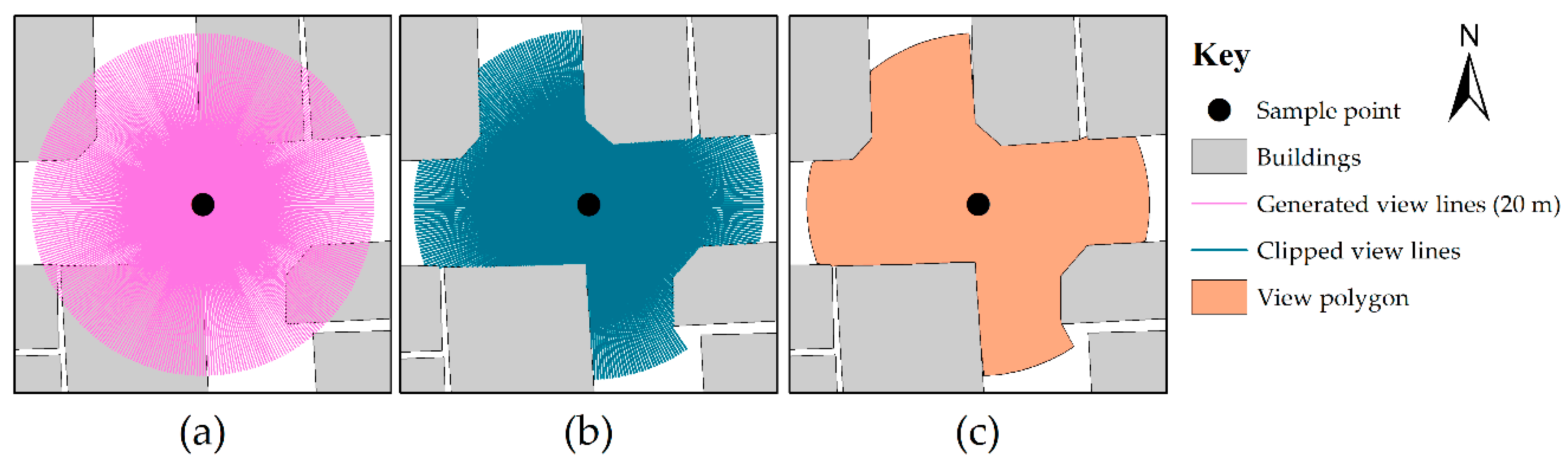
To model the behavior of the laser scanner and localization process, two auxiliary layers were produced: view lines and view polygons. Firstly, for each sample point, 360 view lines, each 20 m in length, radiating outwards from the center at 1° interval, were generated (Figure 3a). These lines represent the laser scanner’s 20 m range. Within the urban environment, the walls of buildings represent a ‘solid’ and opaque barrier for the laser scanner. As 2D GI was used, it is assumed that buildings are infinitely tall, and view lines were clipped where they intersect with the building layer (Figure 3b). This assumption was based on the 30° vertical field of view (+/− 15° up and down) of the Velodyne VLP-16. Mounted at 2.45 m, and with a laser range of 20 m, the effective vertical view is between 0 to 7.8 m. This is equivalent to an average two-story building. Considering the buildings in the experiment area were, at a minimum, three stories high, this assumption was acceptable. Secondly, from these clipped view lines, a minimum bounding convex hull was generated as an areal representation of what the laser scanner ‘sees’ and is referred to as a view polygon (Figure 3c).

5.1.2. Feature Count

The first factor is the feature count. It is an adaption of Javanmardi et al.’s [4] factor, providing a simple count of all nearby features. However, unlike 3D ND map formats, there are three geometry primitives for 2D vector mapping: points, lines, and polygons. Further, the 3D nature of the scanner must be abstracted in 2D.

To account for the differences between the geometric representations, feature count was calculated based on the intersection points between the layer and the view lines or view polygons. For buildings, feature count was the total number of view lines which intersected with the buildings layer. In this scenario, the intersection points were also the endpoints of the view lines as they were previously clipped (as described in Section 5.1). For polygon barriers, points at 10 cm intervals were generated along the intersection with view lines. These generated points were then counted for the feature count. For line barriers, all intersection points between all view lines and line barriers were counted. For point barriers, this was a simple count of features which intersected with (and were therefore within) the view polygon.

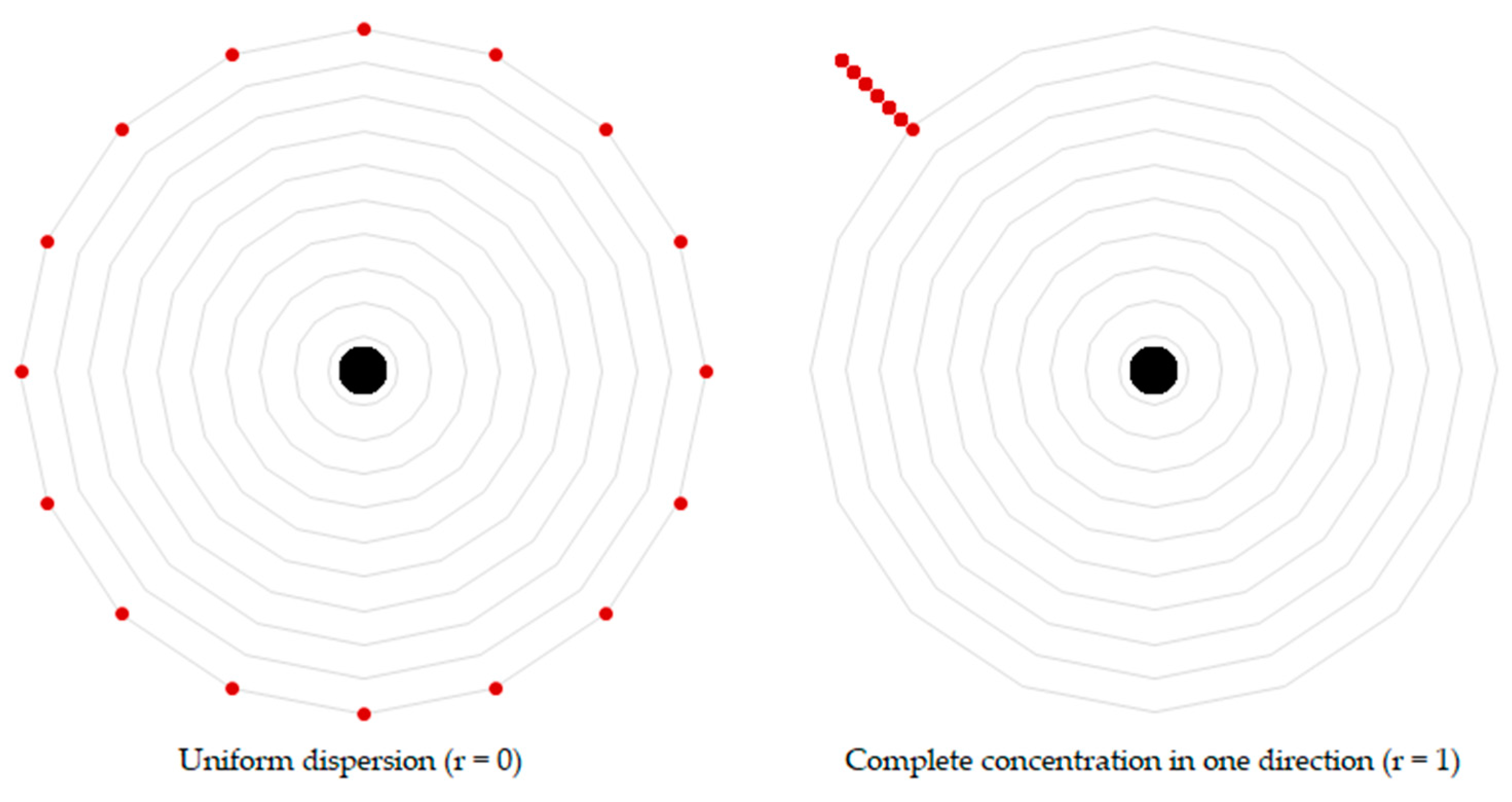
5.1.3. Angular Dispersion of Features

Angular dispersion is a measure of the arrangement of features around the sample point. Akin to Javanmardi et al.’s [4] Feature dilution of precision measure (which in turn was inspired by geometric dilution of precision as used in satellite navigation and global positioning systems). The concept for this factor is that if the nearby features are spread apart rather than close together, it should return better positional accuracy during map matching. This factor describes the uniformity of dispersion and is calculated as follows:

$$Angulardispersion=\sqrt{{\left(\frac{{\displaystyle \sum }\sin \alpha }{n}\right)}^2+{\left(\frac{{\displaystyle \sum }\cos \alpha }{n}\right)}^2}$$

where α is the azimuth of the features, in radians. The factor returns a value between 0 and 1, with a value of 0 indicating a uniform dispersion and a value of 1 meaning a complete concentration in one direction (Figure 4). For this factor, the dispersion of the intersection points between the view lines or view polygons and the respective layer was calculated.

5.1.4. View Line Mean Length

For each sample point, the mean length for every view line which intersected with the building layer was calculated. Non-intersecting view lines were not considered as they would skew the metric. The metric provides an indication if building features in the vicinity are close or far away. A short view line mean length suggests that there are building features nearby, providing elements (e.g., window edges, building corners) to localize against during map matching.

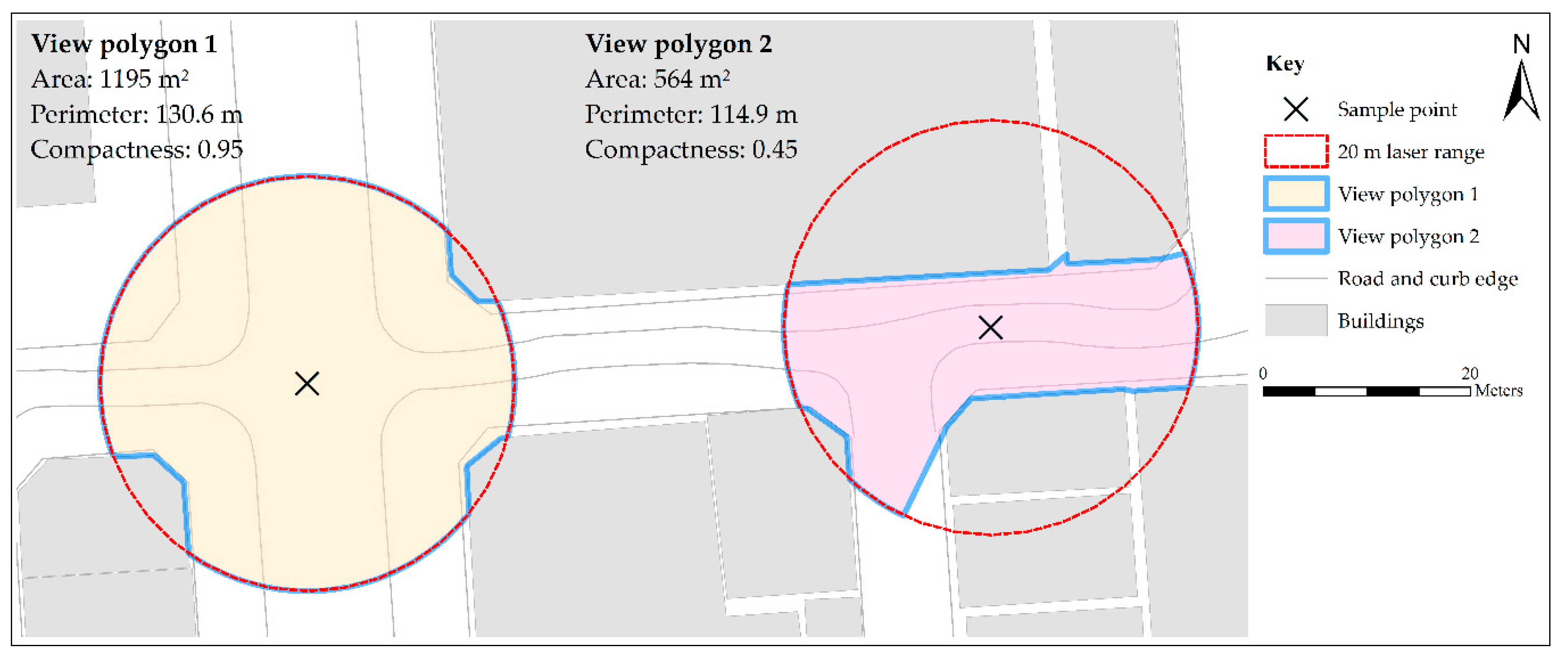
5.1.5. Area of View Polygon

This is the area of the view polygon (as described in Section 5.1). It represents the theoretical area that the laser scanner can ‘see’. Similar to the view line mean length, a small area suggests that there are many building features nearby, with elements to localize against (Figure 5).

5.1.6. Perimeter of View Polygon

This is the perimeter of the view polygon. The premise is that in areas with many features in the vicinity (which is beneficial for localization), the view polygon will have many undulations, resulting in a larger perimeter. Conversely, where there are few features, the perimeter will be small.

5.1.7. Compactness of View Polygon

To measure compactness, the ratio between the area of the view polygon and the area of a circle with the same radius was calculated. A low compactness could suggest that there are many buildings features nearby, providing plenty of stable features and building elements to localize against. Conversely, a high compactness could suggest that there are not many building features in the vicinity. In addition, due to the spread of the laser scanner, closer features are captured at a higher resolution than those which are further away. At longer distances, the laser scanner may not be able to capture the finer details of a building’s façade for localization. Figure 5 illustrates how area, perimeter and compactness can vary along the experiment path.

5.1.8. The Variance of Building Face Direction

Javanmardi et al. [4] suggest that if the features in the local vicinity face a greater variety of directions, then the positioning uncertainty decreases. To measure this, at all points of intersection between the view lines and the building layer, the normal of the face was calculated. Subsequently, for each sample point, the variance of all the normal vectors was calculated.

6. Materials and Methods

6.1. Study Area

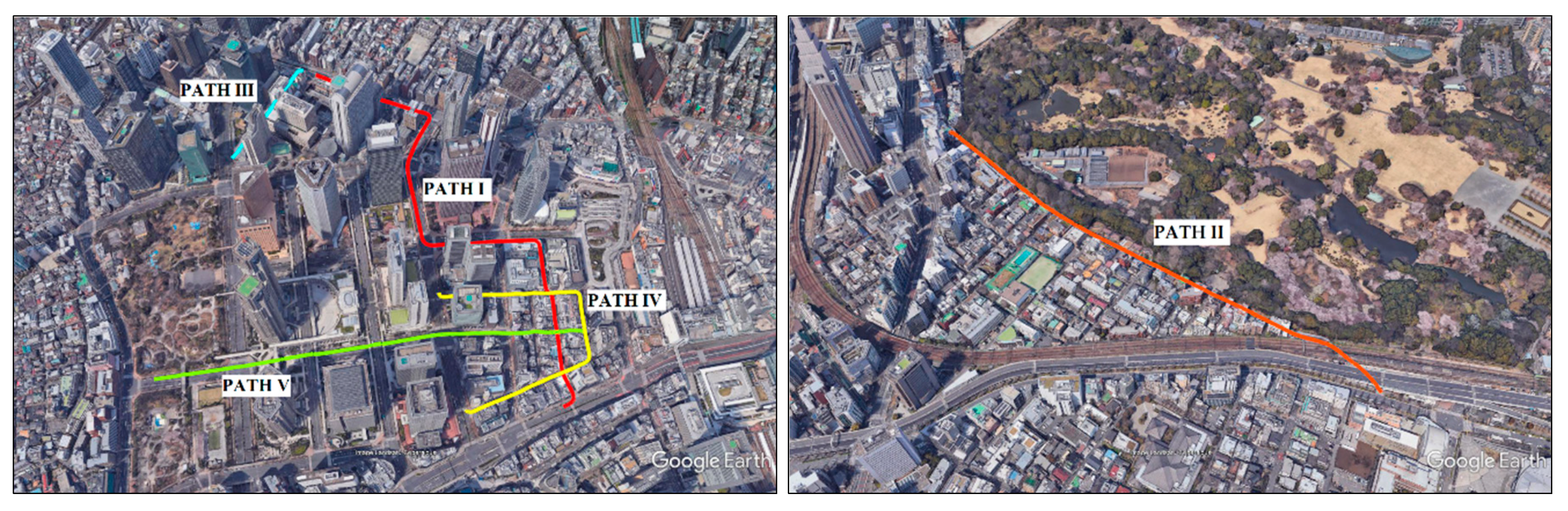
The study area is Shinjuku, Tokyo, Japan. The architecture is relatively heterogeneous, with buildings ranging from low-rise shops to multi-story structures. Similarly, roads vary from single narrow lanes to wide multi-lane carriageways. Five experiment paths were selected to represent a range of environmental configurations, as shown in Figure 6.

Table 2. Summary of all paths.

Path	Length	Description
I	1.16 km	The path begins through a narrow and dense shopping area populated with buildings two to four stories tall. The middle and final third of the path consists of wide roads (two to three lanes), with hedges and trees along the roadside and central reservation, passing by several skyscrapers.
II	0.73 km	A long straight path passing through a residential area. The path begins by passing under a railway bridge. After, residential buildings can be found on the left. On the right, there are no buildings. Instead, there is a metal fence separating the road and the Shinjuku Gyoen National Garden.
III	0.27 km	The shortest of the five paths. This straight path passes between a number of skyscrapers. While the drivable portion of the road is narrow, the pavements are wide and are populated with bollards, trees and lamp posts.
IV	0.65 km	This path is fully contained with the same narrow and dense shopping area found at the beginning of Path I.
V	0.79 km	This long straight path starts in the narrow and dense shopping area from Paths I & IV, before opening to wider, multi-lane roads for the remaining 4/5th of the path. The path passes by a number of skyscrapers in the latter portion, as well as passing under four bridges.
Total	3.60 km

shows a summary and description of all the experiment paths.

6.2. Mapping Data

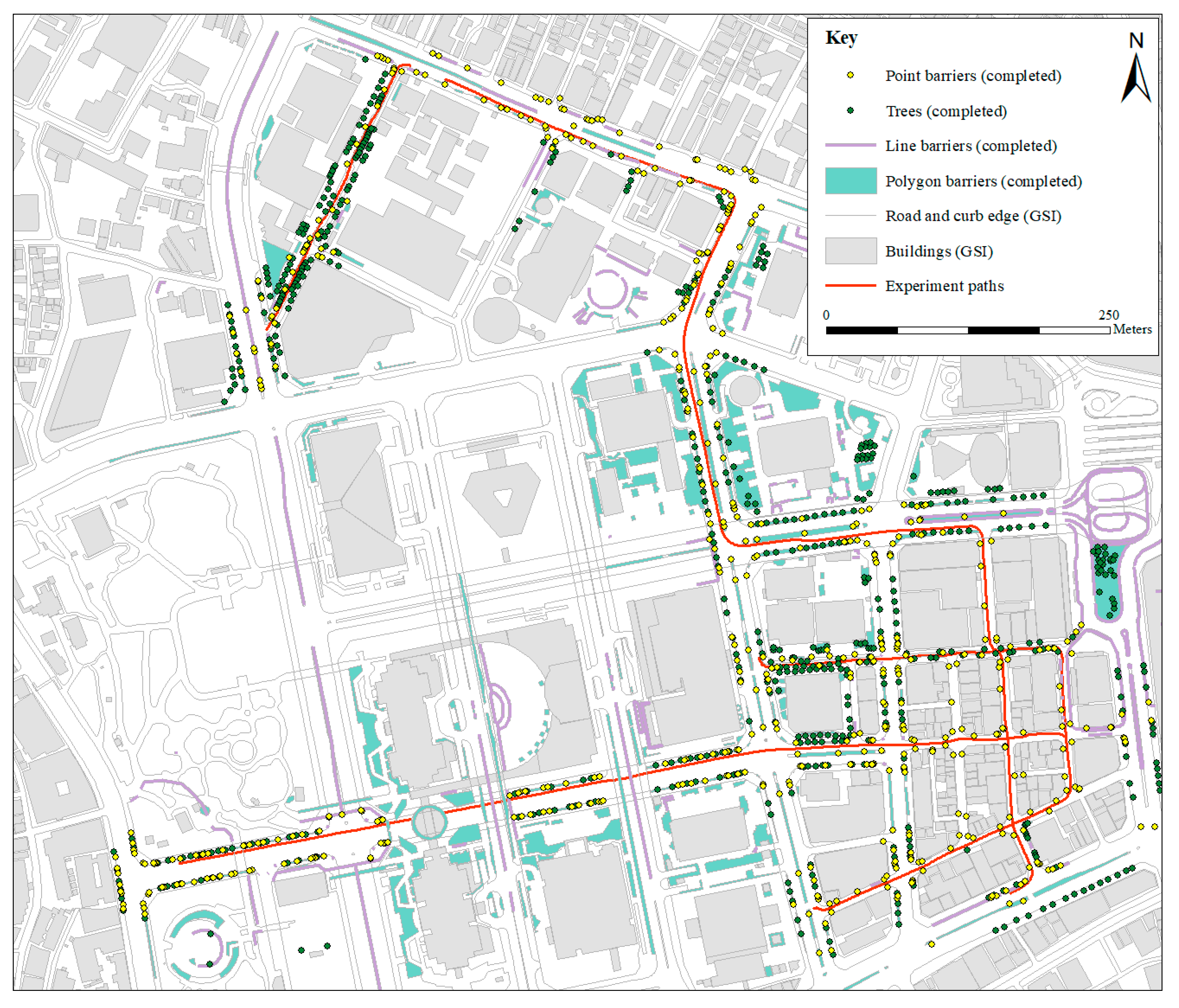
Mapping data from two sources were used in this study: GSI Japan and OSM. As described in Section 3.1, GSI is the national mapping agency of Japan and provides an authoritative source of mapping data. However, while this source of authoritative data is open in Japan, in other countries, mapping data from national mapping agencies are not always freely available. As such, OSM data is also used in this study. Despite the differing levels of data quality and consistency (as highlighted in Section 3.2), OSM still presents a viable and useful source of geospatial data. The specific datasets used from GSI and OSM are described below. Figure 7 and Figure 8 depicts the different mapping data used in this study.

6.2.1. GSI Topographic Map (1:25,000)

Data was downloaded from the GSI mapping portal (http://maps.gsi.go.jp/) in a GML format. For the study area, 20 layers were available, including administrative areas, ground control points, and railway lines. Specifically, for this experiment, building footprints, road line and road edge were extracted. The road line and road edge were combined into a single layer.

6.2.2. OpenStreetMap

Mapping data from OSM was extracted from the geofabrik.de server. For the study area, 49 data layers (referencing 23 tags) were available. Note that each tag can be represented by a maximum of three layers, one for each geometry primitive (point, line, polygon).

Table 3. OSM tags and feature count in the study area.

OSM Tags	Feature Count	OSM Tags	Feature Count
aeroway	11	natural	811
amenity	2468	office	47
barrier	735	place	8
boundary	18	power	21
building	12,434	public transport	161
craft	2	railway	553
emergency	14	route	99
highway	5407	shop	645
historic	21	tourism	199
landuse	230	unknown	690
leisure	143	waterway	5
man made	18

shows a summary of all the tags found in the study area and their feature counts.

Note that OSM tags can represent geometric or semantic features. For example, features labeled as ‘building’ may represent the physical walls of the structure, whereas a ‘boundary’ feature may represent an administrative region, e.g., ward boundary. For this experiment, the aim is to model what the LiDAR scanner ‘sees’ during the localization phase. As such, only the geometric features from OSM are useful.

To model the surrounding environment, five OSM data layers were used: 1) building_polygon; 2) barrier_polygon; 3) barrier_line; 4) barrier_point, and; 5) natural_point. The buildings layer was selected as they represent the most stable feature within the urban landscape. Buildings, in general, are least affected by seasonality or time of day (unlike other features such as trees). For vehicle localization, however, the use of buildings alone for map matching may be insufficient. For example, on wide multi-lane roads or within the rural environment, buildings may not be present or visible by the LiDAR scanner. In these scenarios, roadside features (such as central reservations, median barriers, guard rails, and pole-like features) become increasingly important for localization. Within OSM, these are classified under the ‘barriers’ tag. Areal features, such as hedges, are classed under ‘barrier_polygon’. Linear features, such as guard rails and traffic barriers, are classed as ‘barrier_line’. Lastly, pole-like features (e.g., bollards) are classed as ‘barrier_point’. Lastly, trees are modeled as point features within OSM and are classed as ‘natural_point’.

The completeness of OSM varies within the study area. For buildings, the data is 65.3% complete when compared to GSI building footprints, using the area as a crude measure. For barriers, an authoritative equivalent dataset is not available for reference. In a visual comparison with aerial imagery, over half of the hedges and central reservations (polygon barriers) are missing along the experiment path. There were no line or point barriers mapped within 20 m of the experiment path (although they were present in the data for the wider study area).

To mitigate any issues of inconsistency and incompleteness (as highlighted in Section 3.2), an additional set of ‘completed’ OSM layers was created. Supplementary data (aerial imagery and base map) from ATEC was used to support the manual digitization. By creating these ‘completed’ layers, it allowed the assessment of the capability of OSM, in a scenario where users had correctly and fully mapped all required features. This allowed for a more robust evaluation, without being hindered by data quality issues. In total, 196 polygon-barriers, 115 line-barriers, 596 point-barriers, and 537 natural points (trees) were manually added along the experiment path.

6.3. Localization Error Data

For localization error, data from a previous experiment was used. Specifically, the mean 3D localization error from map matching using a LiDAR input scan and a prebuilt normal distribution (ND) map with a 2.0 m grid size. The process of obtaining the mean 3D localization error is described below. Firstly, a point cloud map of the area was captured using a Velodyne VLP-16 mounted on the roof of a vehicle at the height of 2.45 m. The vehicle speed was limited to 2 m/s, with a scanner frequency of 20Hz to mitigate motion distortion. From this point cloud map, an ND map was generated with a 2.0 m grid size. Next, during the localization phase, a second scan was obtained with the laser scan range limited to 20 m. This second scan was then registered to the ND map (NDT map matching) to obtain a location. Thirdly, to evaluate the map factors, sample points along the experiment path at 1.0 m intervals were selected. For each sample point, mean 3D localization error was calculated by averaging the localization error from 441 initial guesses at different positions evenly distributed around the sample point, at 0.2 m intervals within a range of 2 m. Further details on the experimental set-up and the creation of the data can be found in reference [4].

6.4. Selecting a Prediction Model

Since localization error is a continuous value, a regression model was required. For this problem, the number of samples was relatively low (3465) and the dimensionality was low (maximum of 17 factors). It was also unknown if one factor was more important than other factors. Considering these conditions, an ensemble learning method was appropriate. In this study, random forest regression was used as the prediction model.

Random forest regression is an ensemble learning method which uses multiple decision trees and bootstrap aggregation to form a prediction. Random forest regression aims to reduce variance in predictions while maintaining a low bias, thus controlling overfitting. For the implementation, scikit-learn (a machine learning Python library) was used. As random forest regression is a supervised learning method, a training dataset was required. For each model, the datasets were split into two parts: training (75%) and test (25%).

Other regression models were also tested (Multi-layer perceptron, Support vector machine, Stochastic gradient descent), but did not achieve comparable results without further intensive manual tuning of the models.

7. Results

7.1. General Results

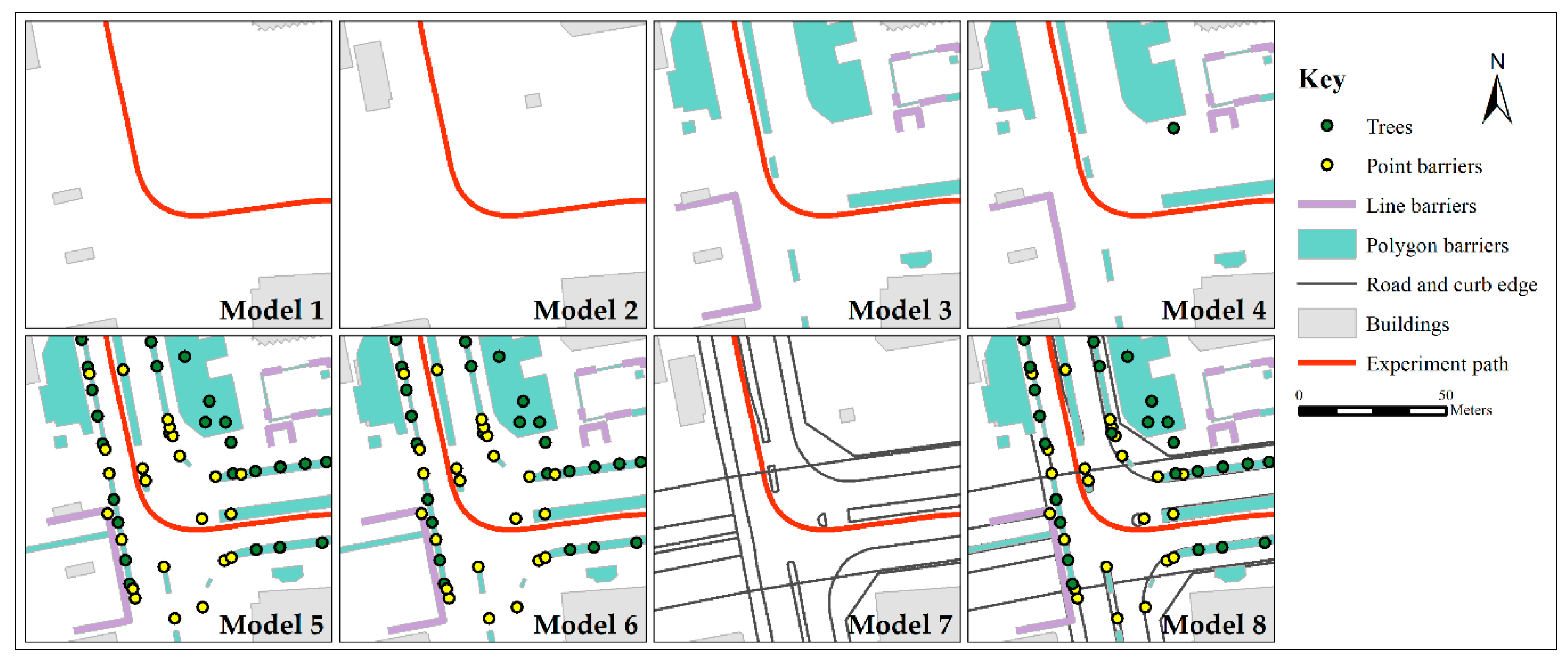
Eight models were evaluated, using different combinations of data from GSI, OSM, and manually digitized layers. Data for all five paths (I/II/III/IV/V) were used together. To begin, Model 1 only used the buildings layer directly from OSM. Similarly, Model 2 used just the building footprints from the GSI Japan topographic map. Model 3 adds the original unedited polygon, line and point barriers to the OSM buildings layer. The original unedited natural points (trees) layer from OSM was then added for Model 4. Model 5 then includes the manually ‘completed’ OSM barriers and natural points layers. Model 6 uses the same completed barriers and natural points layers as Model 5, but replaces the OSM building footprints with GSI data. Model 7 uses just GSI data: building footprints, and combined road and curb edge. Lastly, Model 8 considers the GSI data, with the addition of the completed OSM barriers and completed natural points layers.

To evaluate the goodness of fit, the adjusted R-squared (R²), root mean square error (RMSE), mean absolute error (MAE), and percentile rank are presented. In this scenario, percentile rank is the share of predictions which are below a certain value, e.g., 55% of predictions are within 2.5 cm absolute error. Percentile ranks are presented for three threshold values: 5 cm, 2.5 cm and 1 cm. The models and their prediction errors are presented in

Table 4. Combination of data layers and the performance (accuracy) of the predictive models.

Data		Models
		1	2	3	4	5	6	7	8
Buildings	OSM Buildings	●		●	●	●
	GSI Buildings		●				●	●	●
Barriers	OSM Polygon barriers			●	●
	OSM Line barriers			●	●
	OSM Point barriers			●	●
	Completed Polygon barriers					●	●		●
	Completed Line barriers					●	●		●
	Completed Point barriers					●	●		●
Curb	GSI road and curb edge							●	●
Trees	OSM Natural Points				●
	Completed Natural Points					●	●		●
Number of factors		7	7	13	15	15	15	9	17
R2 (adjusted)		0.26	0.28	0.39	0.40	0.68	0.67	0.50	0.65
RMSE [cm]		7.47	6.60	6.79	6.76	4.96	4.50	5.51	4.59
MAE [cm]		4.19	4.08	3.51	3.48	2.66	2.61	3.09	2.59
Percentile rank (5 cm) [%]		75.1	72.6	81.5	81.5	88.3	87.1	84.4	87.4
Percentile rank (2.5 cm) [%]		48.6	47.2	59.7	60.0	68.4	68.8	62.9	69.8
Percentile rank (1 cm) [%]		24.6	22.3	32.8	32.1	35.4	36.2	32.5	36.9

.

Table 4 shows the combination of data layers used and the performance of the eight predictive models. In Model 1, where only OSM building footprints were used, 48.6% of the estimations have an error below 2.5 cm. Similarly, Model 2 achieved a similar result (47.2%) when only GSI building footprints were used. With the introduction of the unedited OSM barriers layers, the performance improves to 59.7%. However, the addition of the unedited OSM natural points layer (trees) only yields a 0.3% increase in performance (60.0%). One possible explanation is that despite the original unedited OSM data having 811 trees, only 61 were within the 20 m laser range of the five experiment paths. By ‘completing’ the barriers and natural points (trees) layer (as described in Section 6.2.2), the performance improves to 68.4% for Model 5. Model 6 uses the same data as Model 5, except for replacing the OSM building footprints with GSI data. This resulted in the slightest increase in performance to 68.8%. Model 7 uses only GSI data, and 62.9% of the estimations had an error below 2.5 cm. Lastly, Model 8 incorporates all the data sources (specifically, GSI building footprints, GSI road and curb edge, and completed barriers and natural points layers), resulting in a performance of 69.8%. The different data layers used in each of the models are illustrated in Figure 9.

7.2. Factor Importance

One of the advantages of random forest regression is the ability to evaluate the importance of different variables used for prediction.

Table 5. Factor importance of the eight predictive models. The two most important factors in each model are emphasized in bold.

Factors		Models
		1	2	3	4	5	6	7	8
Feature count	Buildings	0.12	0.15	0.07	0.07	0.04	0.07	0.08	0.06
	Polygon barriers	-	-	0.10	0.10	0.18	0.15	-	0.07
	Line barriers	-	-	0.10	0.10	0.11	0.08	-	0.05
	Point barriers	-	-	0.00	0.00	0.04	0.05	-	0.03
	Natural point (trees)	-	-	-	0.01	0.08	0.12	-	0.06
	Road and curb edge	-	-	-	-	-	-	0.38	0.27
Angular dispersion	Buildings	0.17	0.14	0.09	0.09	0.05	0.04	0.06	0.03
	Polygon barriers	-	-	0.12	0.12	0.07	0.06	-	0.07
	Line barriers	-	-	0.17	0.17	0.08	0.08	-	0.04
	Point barriers	-	-	0.00	0.00	0.08	0.08	-	0.04
	Natural point (trees)	-	-	-	0.01	0.05	0.02	-	0.02
	Road and curb edge	-	-	-	-	-	-	0.20	0.09
Other	View line mean length	0.17	0.14	0.09	0.08	0.05	0.05	0.05	0.03
	View polygon area	0.11	0.09	0.06	0.05	0.04	0.03	0.03	0.02
	View polygon perimeter	0.15	0.17	0.07	0.07	0.04	0.05	0.11	0.07
	View polygon compactness	0.11	0.09	0.06	0.06	0.04	0.03	0.03	0.02
	Variance of building face dir.	0.17	0.21	0.08	0.08	0.05	0.08	0.07	0.05

shows an overview of the importance of each factor and data layer, with the two most important variables in bold. For Models 1 and 2, when there are only buildings available, the variance of building face direction is the most important factor. As the barrier features were introduced in Models 3–6, their angular dispersion and feature count have high importance. Note that for trees, when introduced in Models 5 and 6, their angular dispersion has relatively low importance, but their feature count is the 2^nd or 3^rd most important factor. Lastly, with the addition of the GSI road and curb edge layer in Models 7 and 8, the angular dispersion and feature count of road and curb edge have very high importance.

7.3. Hyperparameter Tuning

One of the techniques for improving the performance of random forest regression models is hyperparameter tuning. For each model, there are a number of hyperparameters which are manually set before training. In the case of random forest, these include the number of features considered by each tree when splitting a node or the number of estimators used. For the results in Section 7.1, a default set of hyperparameters were used for all models. These hyperparameters, however, may not be optimal for each model. As such, random search and grid search cross-validation was carried out in order to identify the optimal hyperparameters for model 8.

Table 6. Model 8 performance after hyperparameter tuning.

Performance	Default	Random Search	Grid Search
R2 (adjusted)	0.65	0.66	0.66
RMSE [cm]	4.59	4.54	4.54
MAE [cm]	2.59	2.54	2.54
Percentile rank (5 cm) [%]	87.4	87.5	87.5
Percentile rank (2.5 cm) [%]	69.8	71.3	71.2
Percentile rank (1 cm) [%]	36.9	38.5	38.3

shows the performance of model 8 after hyperparameter tuning. Note that a marginal performance increase (~1.5%) can be achieved.

7.4. Model 8 in Detail

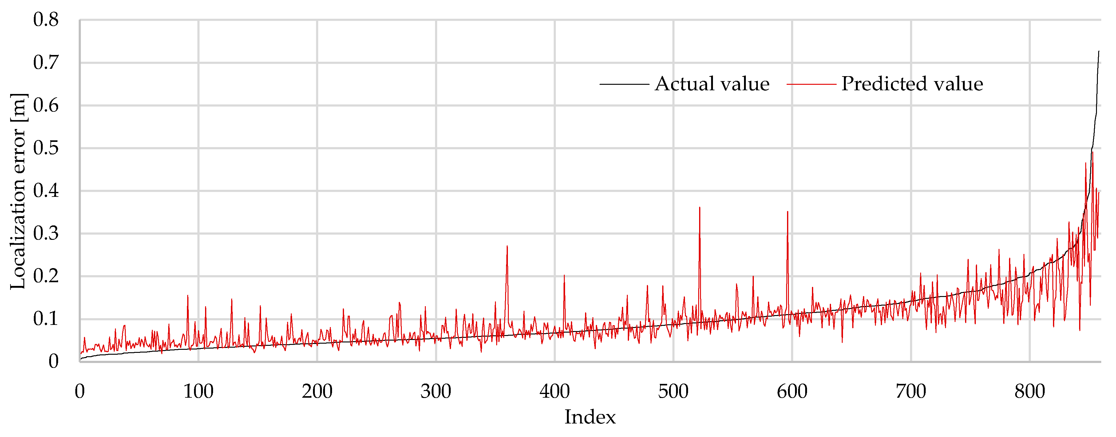
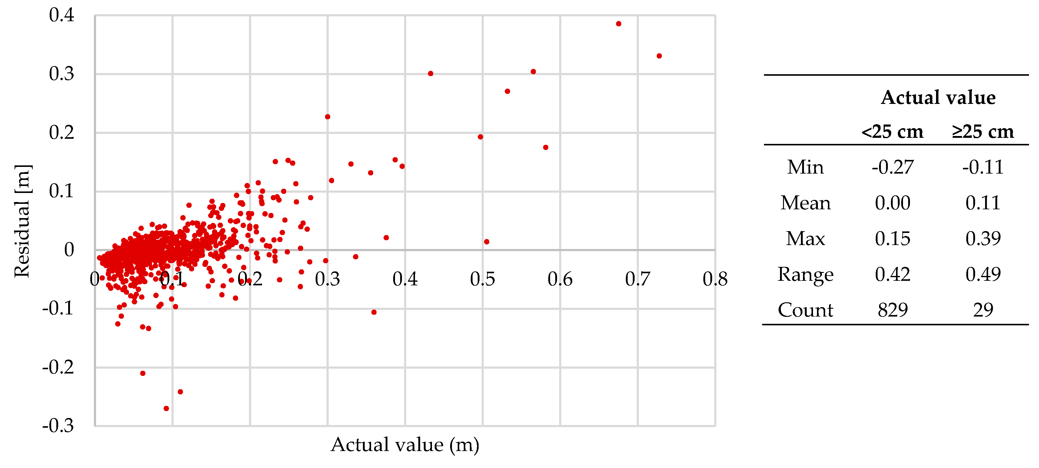
The following subsection presents a closer inspection into model 8. Note that the results in this subsection are using the hyperparameter tuned model 8. Figure 10 shows the predicted localization error in red, against the actual localization error in black. Note that at higher values of localization error (>20 cm), the model is underpredicting. Inspecting the residuals in Figure 11, this becomes much more apparent – for low values of localization error (0–25 cm), the model is performing relatively well, with a mean absolute error of around 0 cm. However, with higher values of localization error (>25 cm), the model can underpredict by up to 39 cm.

7.5. Individual Paths

For Section 7.1, data from all five experiment paths were used simultaneously to train and test the models. However, each of the five paths has different architectural and road side characteristics (as described in Section 6.1 Table 2). For example, while one path may have many buildings and trees within the laser scanner range, others may have none.

Table 7. Mean number of intersection points with features per path point, split by path. The highest value for each feature is highlighted in bold.

Features	Path
	I	II	III	IV	V
Buildings	244.4	258.4	253.7	296.0	222.6
Polygon barriers	4981.5	261.2	2069.2	1158.4	4011.2
Line barriers	42.0	169.6	13.5	29.2	30.2
Point barriers	4.6	2.6	4.1	5.3	4.8
Natural point (trees)	2.4	3.5	13.6	4.7	3.2
Road and curb edge	263.3	327.4	333.5	306.4	245.2
Path length [km]	1.2	0.7	0.3	0.7	0.8
Path points	1096	715	270	631	753

shows the mean count of intersection points with different features along each path. For example, while Path III has a high number of trees along its path (13.6), it has the relatively lowest number of line barriers (13.5).

In order to assess the capability of the map factors within different architectural and roadside scenarios, data for each experiment path was used to train and test individual random forest regression models. The performance of each model is presented in

Table 8. Result of training and testing individual paths, based on model 8.

Performance	Path
	I	II	III	IV	V
Number of factors	17	17	17	17	17
R2 (adjusted)	0.60	0.75	0.53	0.51	0.79
RMSE [cm]	0.03	0.05	0.03	0.51	0.03
MAE [cm]	0.02	0.03	0.02	0.03	0.02
Percentile rank (5 cm) [%]	92.0	88.7	94.1	86.7	91.8
Percentile rank (2.5 cm) [%]	70.1	72.9	66.2	69.0	79.1
Percentile rank (1 cm) [%]	34.3	39.6	32.4	29.1	47.3

. Path V offers the best performance, with 79.12% of estimations within 2.5 cm. Paths I, II, III, and IV offer similar performance, with around 66-73% of estimations within 2.5 cm. In addition, the factor importance for each model is presented in

Table 9. Factor importance, individual paths. The two most important factors for each path are emphasized in bold.

Factors		Path
		I	II	III	IV	V
Feature count	Buildings	0.02	0.06	0.02	0.05	0.01
	Polygon barriers	0.05	0.00	0.05	0.03	0.09
	Line barriers	0.07	0.04	0.28	0.14	0.03
	Point barriers	0.03	0.04	0.01	0.02	0.03
	Natural point (trees)	0.03	0.08	0.02	0.04	0.01
	Road and curb edge	0.34	0.10	0.28	0.03	0.47
Angular dispersion	Buildings	0.02	0.03	0.01	0.04	0.04
	Polygon barriers	0.05	0.01	0.02	0.12	0.05
	Line barriers	0.03	0.02	0.14	0.03	0.09
	Point barriers	0.08	0.02	0.03	0.10	0.04
	Natural point (trees)	0.03	0.09	0.01	0.04	0.01
	Road and curb edge	0.12	0.20	0.02	0.04	0.07
Other	View line mean length	0.02	0.03	0.01	0.05	0.02
	View polygon area	0.01	0.01	0.01	0.03	0.01
	View polygon perimeter	0.04	0.03	0.07	0.08	0.02
	View polygon compactness	0.01	0.01	0.01	0.03	0.01
	Variance of building face dir.	0.03	0.23	0.01	0.13	0.02

.

8. Discussion

The work described in this paper demonstrates that it is possible to estimate autonomous vehicle localization error using 2D geographic information. The general results from Section 6.1 show that in order to adequately model localization error, building footprint data, as well as streel level assets (trees, curbs, barriers), are required. As could be expected, the inclusion of higher quality and more complete data result in better model performance. By ‘completing’ the OpenStreetMap data and addressing issues of incompleteness and inconsistency, model performance improves from 60.0% to 68.4%. Furthermore, with the inclusion of road and curb edge data in Model 8 alongside completed trees data and completed barriers data, it is possible to estimate autonomous vehicle localization, with 69.8% of estimations with an error smaller or equal to 2.5 cm. In addition, through hyperparameter tuning, the performance can be increased to 71.3%. The results obtained indicate that 2D geographic information can be a useful source of spatial data and can be used as a proxy to estimate map-based localization error of an autonomous vehicle.

8.1. The Impact of Different Data Layers and Factors

Within this study, six different data layers were used in conjunction with seven different factors. Inspecting the feature importance across Models 1 to 6 in Table 5, there was no obviously dominant data layer or factor for predicting localization error. However, in Models 7 and 8, the feature count (0.38 and 0.27) and angular dispersion (0.20 and 0.09) of road and curb edges become the most important. One possible explanation is that, of all the data layers, road and curb edge is almost ubiquitously available at all sample points. In contrast, there may not always be trees or buildings within the laser scanner’s 20 m range.

When inspecting the paths individually, however, there is again, no clear data layer or factor which is dominant (Table 7). It can therefore be argued that the importance of different data layers (and their respective factors) are highly dependent on the architecture and street-level assets of the environment. Further work is required to ascertain the scenarios where certain data layers and factors are more useful, e.g., in multi-lane highways, pole-like features are the most important or in narrow single lane alleyways, the variance of building face direction is most useful.

It is important to bear in mind that the factors are calculated individually for different data layers, i.e., there is one factor for the dispersion of buildings and there is another, separate factor for the dispersion of trees. This was designed to assess if certain real-world phenomena are more useful and important for localization than others. This approach could present a potential flaw, as map matching localization using LiDAR data considers all features at the same time, agnostic of what the feature is. For example, in a situation where a road is lined with trees on the left side of the road, and lamp posts on the right, the current factors would indicate a relatively poor angular dispersion when calculated individually for each layer. However, if considered together, it would reflect a more uniform dispersion of features. Further work is therefore required to refine the map evaluation factors in order to consider the features in the vicinity more holistically.

8.2. The Impact of 2D Geographic Information Representation

In this study, 2D geographic information in a vector format was used instead of a 3D point cloud map to predict localization error. One of the main differences is that 2D GI is a much more abstracted representation than a 3D point cloud map. As mentioned in Section 3, 2D geographic information in a vector format data can be represented using three geometric primitives: points, lines, and polygons. From a data handling and computation perspective, it is much ‘lighter’. The vector geometry also provides clear boundaries for delineating features, which is not found in point cloud maps. This makes it easier to model ‘opaque’ features such as buildings which the LiDAR scanner cannot ‘see’ through.

The main drawback of 2D GI is that it lacks the detail found within a 3D point cloud and the high level of abstraction. Here, it is important to note that some phenomena are better represented as 2D vector data than others. For example, while a crash barrier can be well represented by a line (from a top-down perspective), it can be argued that a tree is ill-represented as a single point. Providing that only a short time has elapsed between the mapping and localization phase, organic features such as trees with its leaves and branches could, in fact, be highly useful features for localization. These feature-level details are often lost in the abstraction to 2D GI, whereas a 3D point cloud (and as an extension, 3D ND maps) do not suffer as much from generalization. Façade detail is also lost in a 2D representation. Further work towards using 3D geographic information may resolve some of the inherent issues of 2D representations. The problem, however, remains of what level of detail is sufficient for the application of autonomous driving. There needs to be a balance between abstraction and performance, in order to create a dataset that is fit-for-purpose.

8.3. Crowdsourced and National Mapping Agency Data

Within this study, both crowdsourced (OpenStreetMap) and national mapping agency (GSI Japan) data were used. When using crowdsourced data, data quality issues such as inconsistency and incompleteness can be a challenge. In this study, OSM data was manually completed using external datasets, resulting in an 8.4% improvement in model performance over using the original OSM data. It is therefore likely as the quality of OSM improves over time, its capacity to estimate localization error accurately also increases.

Mapping data from GSI Japan, the national mapping agency, was also used in this study. Despite the consistency and completion disparity between the crowdsourced OpenStreetMap data and the national mapping agency GSI Japan data, it was somewhat surprising to find that there was no substantial difference in performance when using the two different sources of data. When using just building footprints, Model 1 which uses OSM data (48.6%) outperforms Model 2 which uses GSI data (47.2%). When the completed barrier layers are also included, using GSI building footprints (68.8%) marginally outperforms using OSM data (68.4%). One possible explanation for this is that for the experiment paths and its vicinity, the completion and consistency of OSM data for building footprints are comparatively high. Should the experiment be replicated in an area where OSM suffers from missing data, it is expected that using GSI data would result in a better modeling performance.

8.4. Comparison with Other Studies

Table 10. Comparison with other models.

Author	Model	R2	RMSE [cm]
Javanmardi et al. [28]	2.0 m grid size	0.770	9.0
	5.0 m grid size	0.551	20.6
Our models	Model 5	0.677	5.0
	Model 8	0.654	4.6

presents a comparison between Model 8 and Javanmardi et al.’s [28] ND map mean error models. Our model can achieve comparable performance with an RMSE of 4.6 cm and an R² of 0.654. Although Javanmardi et al.’s [28] 2.0 m model has a higher R² value (0.77), the RMSE is much higher at 9.0 cm. It is important to bear in mind the difference in methodology—while [28] uses principal component regression, this study uses random forest regression. Caution must be taken with this comparison, as a simple comparison of RMSE and R² is not enough to ascertain if one model performs better than another in practice. Further work is required to ascertain the different model’s ability to detect points where localization error exceeds the threshold value (This is discussed further in Section 8.6).

8.5. Generalizability of the Model

One of the main objectives of this study was to exploit 2D geographic information’s availability and wide coverage for the estimation of the localization error. One potential practical application was to train the model with enough data such that it would then be possible to predict localization error beyond the modeled area. The addition of sufficient training data should help reduce any random patterns that may previously have appeared predictive. Provided 2D geographic information is readily available, it could then be theoretically possible to predict localization error for any location. Subsequently, the generalizability of the model must be thoroughly assessed and validated.

8.6. Practical Implications

The results from this study show that it is possible to estimate localization error using 2D geographic information, with 69.8% of estimates within 2.5 cm and 87.4% within 5 cm. While these results are encouraging, further investigations into Model 8 show that the current approach tends to underpredict in areas of high localization error. For the application of autonomous vehicles, it can be argued that detecting the points which exceed a threshold error value is perhaps more important than the general accuracy of the prediction. This is because, at these locations, the vehicle is unable to localize itself within a safety threshold.

Inspecting the residual plot for Model 8, the model is effective at predicting for low values of localization error (<25 cm), with a mean residual of 0 cm. However, for higher values of localization error (≥25 cm), the model can underpredict by 39 cm. This could be attributed to the lack of training data for areas of high localization error. Of the 2571 points within the training data, only 100 points (3.9%) had a localization error higher than 25 cm (

Table 11. Distribution of actual localization error, by count (Model 8).

Localization Error	All	Test	Training
0.0 ≤ x < 0.2	3179	797	2382
0.2 ≤ x < 0.4	207	53	154
0.4 ≤ x < 0.6	28	6	22
0.6 ≤ x	15	2	13
Total	3429	858	2571
Localization error higher than 25 cm	129	29	100

). In practice, this can be an issue, as within the application of autonomous driving, the effective and accurate detection of these threshold exceedance points is critical to safety. Further work is therefore required to capture more training data where localization error is high, as well as designing a prediction model which is effective at detecting these peaks in localization error.

8.7. Source of Localization Error

As described in Section 2.2, there are many sources of localization error for LiDAR map matching. The precise sources of localization error, however, remain difficult to ascertain. Within the study, multiple measures were taken to ensure the reduction of non-map errors, so that any remaining localization error evaluated was directly related to the map as much as possible. Regardless, it is currently difficult to confirm how much of the localization error was derived from the map or the environment. In the future, if the source of localization error is known, map producers could be encouraged to improve mapping for the application of localization. Alternatively, artificial objects could be installed in the environment to improve map matching performance.

9. Conclusions

This study set out to determine if 2D geographic information can be used as a proxy to estimate vehicle localization error. Seven map evaluation factors were developed for 2D geographic information in a vector format, based on the feature sufficiency and layout of the map. Using these factors, eight random forest regression models were trained using a combination of OSM, GSI Japan, and manually digitized mapping data for five experiment paths in Shinjuku, Tokyo. The results of this investigation show that it is possible to predict 69.8% of localization error within 2.5 cm and 87.4% within 5 cm. Further work is required in capturing more training data for areas of high localization error, as well as refining the models to better detect peaks and avoid underprediction.

References

- Ellul, C.; Adjrad, M.; Groves, P. The Impact of 3D Data quality on Improving GNSS Performance Using city Models Initial Simulations. ISPRS Ann. Photogramm. Remote Sens. Spat. Inf. Sci. 2016, IV-2/W1, 171–178. [Google Scholar] [CrossRef]
- Levinson, J.; Thrun, S. Robust vehicle localization in urban environments using probabilistic maps. In Proceedings of the 2010 IEEE International Conference on Robotics and Automation, Anchorage, AK, USA, 3–7 May 2010; pp. 4372–4378. [Google Scholar]
- Javanmardi, M.; Javanmardi, E.; Gu, Y.; Kamijo, S.; Javanmardi, M.; Javanmardi, E.; Gu, Y.; Kamijo, S. Towards High-Definition 3D Urban Mapping: Road Feature-Based Registration of Mobile Mapping Systems and Aerial Imagery. Remote Sens. 2017, 9, 975. [Google Scholar] [CrossRef]
- Javanmardi, E.; Javanmardi, M.; Gu, Y.; Kamijo, S. Factors to Evaluate Capability of Map for Vehicle Localization. IEEE Access 2018, 6, 49850–49867. [Google Scholar] [CrossRef]
- Akai, N.; Morales, L.Y.; Takeuchi, E.; Yoshihara, Y.; Ninomiya, Y. Robust localization using 3D NDT scan matching with experimentally determined uncertainty and road marker matching. In Proceedings of the 2017 IEEE Intelligent Vehicles Symposium (IV), Los Angeles, CA, USA, 11–14 June 2017; pp. 1356–1363. [Google Scholar]
- International Organization for Standardization (ISO) ISO 17572-1:2015 - Intelligent Transport Systems (ITS)—Location Referencing for Geographic Databases—Part 1: General Requirements and Conceptual Model. Available online: https://www.iso.org/standard/63400.html (accessed on 24 May 2019).
- International Organization for Standardization (ISO) ISO 17572-2:2018 - Intelligent Transport Systems (ITS)—Location Referencing for Geographic Databases—Part 2: Pre-coded Location References (Pre-coded Profile). Available online: https://www.iso.org/standard/69468.html (accessed on 24 May 2019).
- Sobreira, H.; Costa, C.M.; Sousa, I.; Rocha, L.; Lima, J.; Farias, P.C.M.A.; Costa, P.; Moreira, A.P. Map-Matching Algorithms for Robot Self-Localization: A Comparison Between Perfect Match, Iterative Closest Point and Normal Distributions Transform. J. Intell. Robot. Syst. 2019, 93, 533–546. [Google Scholar] [CrossRef]
- Magnusson, M. The three-dimensional normal-distributions transform: an efficient representation for registration, surface analysis, and loop detection. Ph.D. Thesis, Örebro Universitet, Örebro, Sweden, 2009. [Google Scholar]
- Magnusson, M.; Lilienthal, A.; Duckett, T. Scan registration for autonomous mining vehicles using 3D-NDT. J. F. Robot. 2007, 24, 803–827. [Google Scholar] [CrossRef] [Green Version]
- Biber, P.; Strasser, W. The normal distributions transform: a new approach to laser scan matching. In Proceedings of the Proceedings 2003 IEEE/RSJ International Conference on Intelligent Robots and Systems (IROS 2003) (Cat. No.03CH37453), Las Vegas, NV, USA, 27–31 October 2003; Volume 3, pp. 2743–2748. [Google Scholar]
- International Organization for Standardization (ISO) ISO 19101-1:2014(en) Geographic Information — Reference Model — Part 1: Fundamentals. Available online: https://www.iso.org/obp/ui/#iso:std:iso:19101:-1:ed-1:v1:en (accessed on 24 May 2019).
- Longley, P.A.; Goodchild, M.F.; Maguire, D.J.; Rhind, D.W. Geographic Information Systems and Science, 4th ed.; John Wiley & Sons, Ltd.: Chichester, UK, 2015; ISBN 1118676955. [Google Scholar]
- De Smith, M.J.; Goodchild, M.F.; Longley, P. Geospatial Analysis: A Comprehensive Guide to Principles, Techniques and Software Tools, 6th ed.; Troubador Publishing Ltd.: Leicester, UK, 2018. [Google Scholar]
- Wieczorek, W.F.; Delmerico, A.M. Geographic Information Systems. Comput. Stat. 2009, 1, 167–186. [Google Scholar] [CrossRef]
- OpenStreetMap Map Features - OpenStreetMap Wiki. Available online: https://wiki.openstreetmap.org/wiki/Map_Features (accessed on 25 March 2019).
- Barrington-Leigh, C.; Millard-Ball, A. The world’s user-generated road map is more than 80% complete. PLoS ONE 2017, 12, e0180698. [Google Scholar] [CrossRef] [PubMed]
- OpenStreetMap WikiProject Japan/Current Coverage - OpenStreetMap Wiki. Available online: https://wiki.openstreetmap.org/wiki/WikiProject_Japan/Current_coverage (accessed on 20 March 2019).
- Zielstra, D.; Zipf, A. A comparative study of proprietary geodata and volunteered geographic information for Germany. In Proceedings of the 13th AGILE International Conference on Geographic Information Science, Guimarães, Portugal, 11–14 May 2010; Volume 2010. [Google Scholar]
- Helbich, M.; Amelunxen, C.; Neis, P.; Zipf, A. Comparative spatial analysis of positional accuracy of OpenStreetMap and proprietary geodata. In Proceedings of the GI_Forum 2012, Salzburg, Austria, 3–6 July 2012; pp. 24–33. [Google Scholar]
- Obst, M.; Bauer, S.; Reisdorf, P.; Wanielik, G. Multipath detection with 3D digital maps for robust multi-constellation GNSS/INS vehicle localization in urban areas. In Proceedings of the 2012 IEEE Intelligent Vehicles Symposium, Alcala de Henares, Spain, 3–7 June 2012; pp. 184–190. [Google Scholar]
- Rahman, K.M.; Alam, T.; Chowdhury, M. Location based early disaster warning and evacuation system on mobile phones using OpenStreetMap. In Proceedings of the 2012 IEEE Conference on Open Systems, Kuala Lumpur, Malaysia, 21–24 October 2012; pp. 1–6. [Google Scholar]
- Bakillah, M.; Liang, S.; Mobasheri, A.; Jokar Arsanjani, J.; Zipf, A. Fine-resolution population mapping using OpenStreetMap points-of-interest. Int. J. Geogr. Inf. Sci. 2014, 28, 1940–1963. [Google Scholar] [CrossRef]
- Hentschel, M.; Wagner, B. Autonomous robot navigation based on OpenStreetMap geodata. In Proceedings of the 13th International IEEE Conference on Intelligent Transportation Systems, Funchal, Portugal, 19–22 September 2010; pp. 1645–1650. [Google Scholar]
- Senlet, T.; Elgammal, A. A framework for global vehicle localization using stereo images and satellite and road maps. In Proceedings of the 2011 IEEE International Conference on Computer Vision Workshops (ICCV Workshops), Barcelona, Spain, 6–13 November 2011; pp. 2034–2041. [Google Scholar]
- Floros, G.; van der Zander, B.; Leibe, B. OpenStreetSLAM: Global vehicle localization using OpenStreetMaps. In Proceedings of the 2013 IEEE International Conference on Robotics and Automation, Karlsruhe, Germany, 6–10 May 2013; pp. 1054–1059. [Google Scholar]
- Vysotska, O.; Stachniss, C. Improving SLAM by Exploiting Building Information from Publicly Available Maps and Localization Priors. PFG – J. Photogramm. Remote Sens. Geoinf. Sci. 2017, 85, 53–65. [Google Scholar] [CrossRef]
- Javanmardi, E.; Javanmardi, M.; Gu, Y.; Kamijo, S. Adaptive Resolution Refinement of NDT Map Based on Localization Error Modeled by Map Factors. In Proceedings of the 2018 21st International Conference on Intelligent Transportation Systems (ITSC), Maui, HI, USA, 4–7 November 2018; pp. 2237–2243. [Google Scholar]
Figure 1.
Excerpt of GSI 1:25,000 base map, as viewed on the GSI web map portal.
Figure 2.
Excerpt of OSM [left] and Geospatial Information Authority of Japan (GSI) base map [right]. Note the inconsistency in completeness for OSM, in contrast to the GSI data.
Figure 3.
The generation of view lines and view polygons. (a) 360 view lines generated, each 20 meter in length, at 1° interval. (b) View lines clipped by building footprints. (c) View polygon generated from the minimum bounding convex hull of the clipped view lines.
Figure 4.
Calculating angular dispersion. The measure describes the dispersion of intersection points (red circles) in relation to the sample point in the center (black circle).
Figure 5.
Two different view polygons and their respective area, perimeter and compactness.
Figure 6.
Five experiment paths (I, II, III, IV, V) in Shinjuku, Tokyo, Japan, as viewed in Google Earth.
Figure 7.
Map showing the completed barriers (point/line/polygon) layer, completed trees layer, GSI building footprints, GSI road and curb edge, and experiment paths I, III, IV, and V.
Figure 8.
Map showing the completed barriers (point/line/polygon) layer, completed trees layer, GSI building footprints, GSI road and curb edge, and experiment path II.
Figure 9.
Maps showing the different data layers in each of the eight models as described in Table 4.
Figure 10.
Predicted (red) vs. actual (black) value of localization error, sorted by actual value (Model 8, test data).
Figure 11.
Residual plot of predicted values against the actual value (Model 8, test data). The table shows the minimum, mean and maximum residual, as grouped by the actual value.