mgwr: A Python Implementation of Multiscale Geographically Weighted Regression for Investigating Process Spatial Heterogeneity and Scale

Abstract

Geographically weighted regression (GWR) is a spatial statistical technique that recognizes that traditional ‘global’ regression models may be limited when spatial processes vary with spatial context. GWR captures process spatial heterogeneity by allowing effects to vary over space. To do this, GWR calibrates an ensemble of local linear models at any number of locations using ‘borrowed’ nearby data. This provides a surface of location-specific parameter estimates for each relationship in the model that is allowed to vary spatially, as well as a single bandwidth parameter that provides intuition about the geographic scale of the processes. A recent extension to this framework allows each relationship to vary according to a distinct spatial scale parameter, and is therefore known as multiscale (M)GWR. This paper introduces mgwr, a Python-based implementation of MGWR that explicitly focuses on the multiscale analysis of spatial heterogeneity. It provides novel functionality for inference and exploratory analysis of local spatial processes, new diagnostics unique to multi-scale local models, and drastic improvements to efficiency in estimation routines. We provide two case studies using mgwr, in addition to reviewing core concepts of local models. We present this in a literate programming style, providing an overview of the primary software functionality and demonstrations of suggested usage alongside the discussion of primary concepts and demonstration of the improvements made in mgwr.

1. Introduction

Geographically weighted regression (GWR) is a spatial statistical technique that, like aspatial local regression, recognizes that traditional ‘global’ regression models may be limited when processes vary by context. GWR captures process’s spatial heterogeneity (i.e., process variation by spatial context) via an operationalization of Tobler’s first law of geography: “everything is related to everything else, but near things are more related than distant things” [1]. An ensemble of local linear models are calibrated at any number of locations by ‘borrowing’ nearby data. The result is a surface of location-specific parameter estimates for each relationship in the model that may vary spatially, as well as a single bandwidth parameter that provides intuition about the geographic scale of the processes. In addition, GWR typically provides increased model fit and reduced residual spatial autocorrelation compared to a traditional ‘global’ regression that assumes relationships are constant over space [2].

A recent extension to the GWR framework allows each relationship in the model to vary at a unique spatial scale and is therefore known as multiscale (M)GWR [3]. MGWR is much less restrictive in its assumptions than GWR, since the relationship between the response and a covariate is allowed to vary locally, vary regionally, and or not vary at all. Eliminating the restriction that all relationships vary at the same spatial scale can minimize over-fitting, reduce bias in the parameter estimates, and mitigate concurvity (i.e., collinearity due to similar functional transformations). Therefore, MGWR has been suggested as the default local model specification when using GWR to investigate process spatial heterogeneity and scale.

This paper introduces mgwr (throughout this manuscript mgwr refers to the software implementation, while MGWR refers to the technique more generally), a Python-based software package for deploying GWR and MGWR models. Though there are existing software options, they are limited in terms of available functionality, computational efficiency, or both. For example, there is a GWR tool in the spatial analyst toolbox within ArcGIS [4] and there are several options within the R ecosystem, such as spgwr [5] and gwrr [6]. However, none of these implementations offers capabilities to calibrate an MGWR model nor the ability to compute the hat matrix (i.e., projection matrix) and the associated novel model diagnostics described in [7], which includes covariate-specific indicators of scale and inference framework. The R-based GWmodel [8] offers some MGWR functionality although the focus is primarily on parameter-specific distance metrics [9] rather than multiple scales of analysis and it also lacks some recent computational enhancements that avoids the storage and manipulation of large numerical arrays hat arise in GWR/MGWR [10]. Consequently, mgwr offers a computationally efficient software package that explicitly focuses on the multiscale analysis of spatially heterogeneous processes. In addition, mgwr compliments R-based free and open source implementations (i.e., spgwr, gwrr, and GWmodel) by offering a Python-based alternative, increasing the overall accessibility of GWR and MGWR tools.

The remainder of this paper is structured as follows. First, where to find the source code, how to install it, and the datasets utilized throughout the paper are discussed. Then, some core GWR concepts are reviewed and illustrated. Next, new concepts and functionality required to deploy the recent MGWR extension and diagnostics are presented. Finally, mgwr is compared to two other software implementations to compare computational efficiency. Throughout the paper, best-practices are suggested and demonstrated on empirical datasets.

2. Source Code and Datasets

2.1. Source Code and Installation

The mgwr source code (the examples in this paper were composed using mgwr version 2.0.1) is organized as a module of the Python spatial analysis library (PySAL) (https://pysal.org) and is therefore available from a repository on the PySAL project GitHub page (https://github.com/pysal/mgwr). Each PySAL module is complete with ‘docstrings’ (i.e., input and output documentation) for all available functions and code examples (i.e., Jupyter notebooks) that make it simple to replicate and extend the examples to new applications. In addition, ‘unit tests’ are provided that allow the source code to be continuously integrated while being developed. This ensures that new features and dependency updates do not unknowingly break existing features.

Currently, mgwr has four dependencies: numpy, scipy, libpysal, and spglm. The first two dependencies, numpy and scipy, are elementary within the Python scientific computing ecosystem and provide core data structures and data manipulation functions. The third dependency, libpysal, is central to PySAL and provides a repository of example datasets. Since libpysal is dependent upon pandas, then pandas is an indirect dependency for mgwr and is often useful for reading and managing data tables. The final dependency, spglm, provides a light-weight generalized linear model framework for calibrating each of the local parameter estimates within (M)GWR via iteratively weighted least squares. The most recent stable version of mgwr, along with these direct and indirect dependencies, may be installed from the Python packaging index (PyPI) using the pip package manager:

pip install mgwr

To obtain in-development features, it is also possible to install mgwr directly from the source code:

pip install https://github.com/pysal/mgwr/archive/master.zip

Additional packages, namely matplotlib and geopandas, are used for presenting results from empirical demonstrations and can also be obtained via pip; however, they are not required for the core mgwr functions. Once all the necessary packages are installed, they can be imported for use in the following examples as such:

>>> import numpy as np

>>> import pandas as pd

>>> import libpysal as ps

>>> from mgwr.gwr import GWR, MGWR

>>> from mgwr.sel_bw import Sel_BW

>>> from mgwr.utils import compare_surfaces, truncate_colormap

>>> import geopandas as gp

>>> import matplotlib.pyplot as plt

>>> import matplotlib as mpl

2.2. Datasets

Two datasets are utilized throughout this paper to illustrate various (M)GWR functionality. First, is the well-known Georgia dataset that is described in [2] (2002) as well as subsequent publications [7,11]. The second is a sample of Airbnb rental data from the Prenzlauer Berg neighborhood of Berlin from InsideAirbnb, which provides a more recent example with a relatively larger sample size.

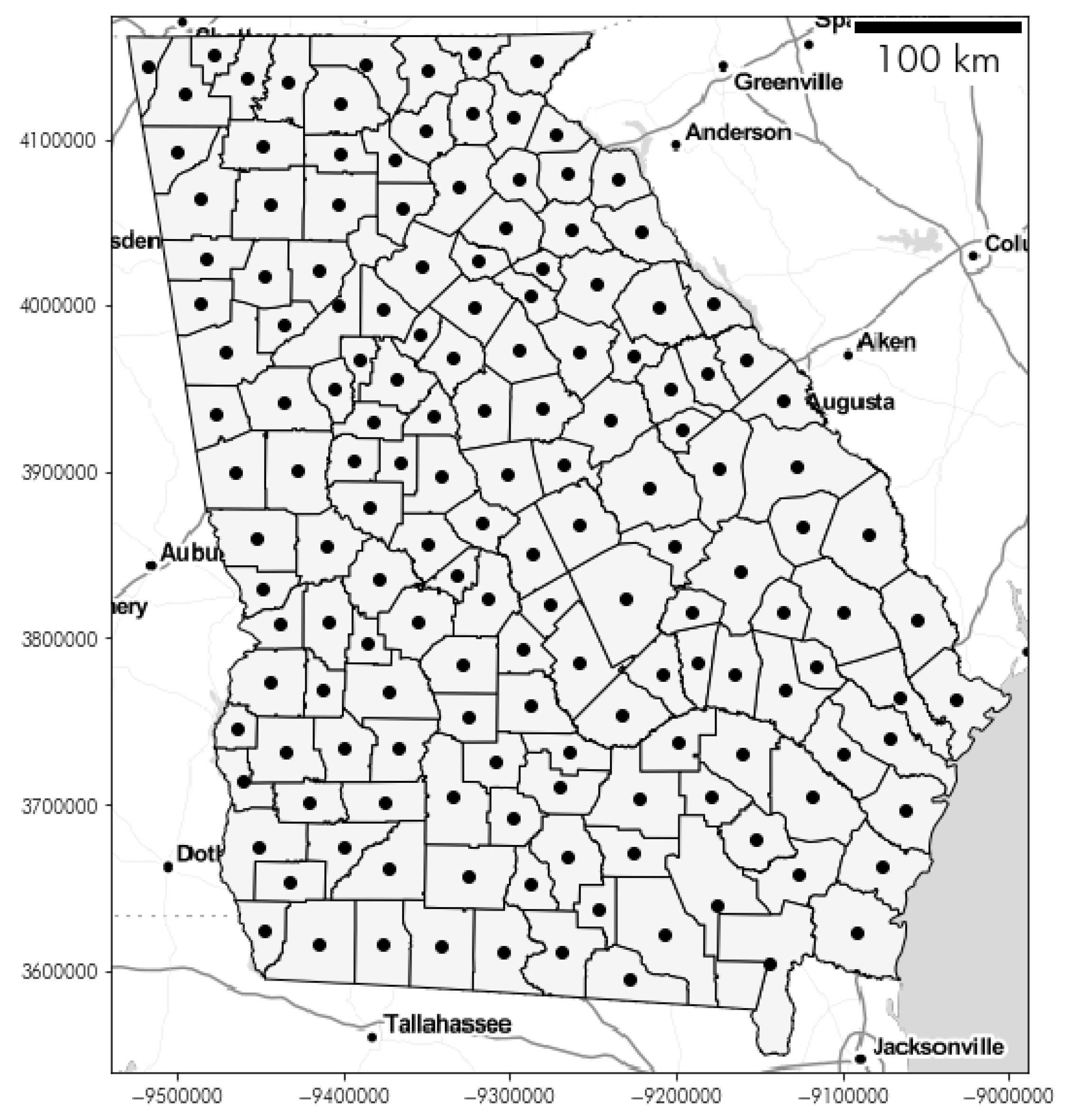
2.2.1. Georgia Dataset

The Georgia dataset consists of 159 counties in the state of Georgia (Figure 1), and records socio-demographic characteristics from the 1990 US census. The county locations are abstracted as centroids so that inter-county distances can be computed within the (M)GWR routine, though it is convenient to visualize the model output using the county polygons, since they are the scale at which the observations are aggregated. A small subset of the available variables are selected here for an example modeling educational attainment. The covariates are described in

Table 1. Georgia dataset.

Short Name	Description
PctBach	Percentage of the population with a bachelor’s degree or higher
PctFB	Percentage of the population that was born in a foreign country
PctBlack	Percentage of the population that identifies as African American
PctRural	Percentage of the population that is classified as living in a rural area

. Python code for loading and visualizing the Georgia dataset is as follows:

#Load Georgia dataset and generate plot of Georgia counties (Figure 1)

>>> georgia = gp.read_file(ps.examples.get_path(‘G_utm.shp’))

>>> fig, ax = plt.subplots(figsize = (10, 10))

>>> georgia.plot(ax=ax, **{‘edgecolor’: ‘black’, ‘facecolor’: ‘white’})

>>> georgia.centroid.plot(ax = ax, c = ‘black’)

>>> plt.savefig(‘georgia_shp’)

>>> plt.show()

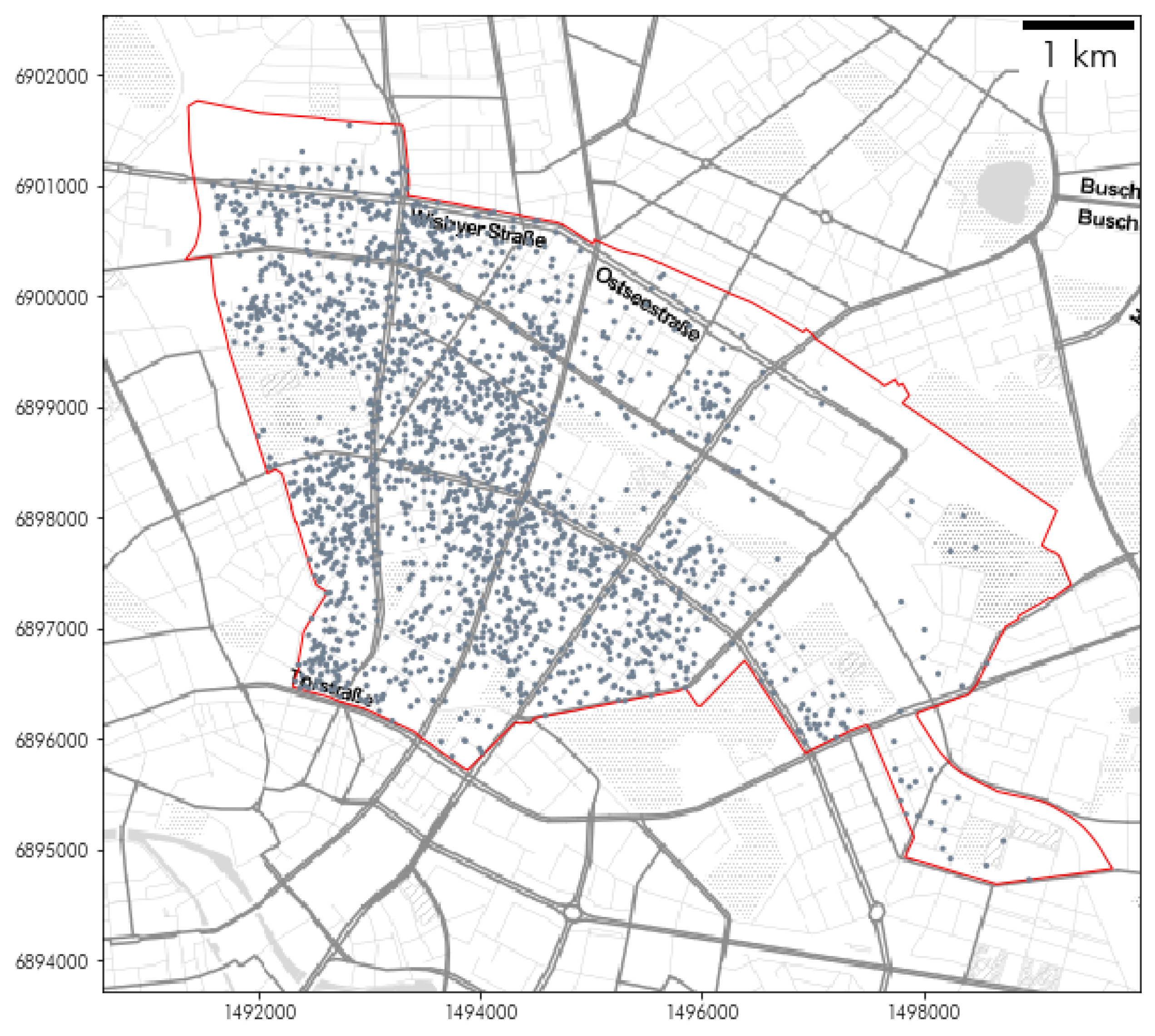
2.2.2. Berlin Airbnb Dataset

The Berlin dataset consists of 2203 observations that are geolocated instances of Airbnb rental properties (Figure 2) and their associated characteristics from 2017 in the Prenzlauer Berg neighborhood. Prenzlauer Berg is a gentrifying neighborhood known for its arts scene, shopping, and nightlife, and is therefore a popular tourist destination. A small subset of variables were selected for a rental price modeling example, which are described in

Table 2. Berlin dataset.

Short Name	Description
Log price	Logged price of rental unit
Score	Cumulative review score from previous customers for each rental unit
Accommodates	Number of individuals a rental unit can accommodate
Bathrooms	Number of bathrooms in each rental unit

. Note that the logarithm of rental price is used here to correct the skewness of the variable. Since the data are not aggregated, the analysis and visualization of the results are carried out at the point-level.

#Load Berlin dataset and generate plot of properties (Figure 2)

>>> prenz = gp.read_file(ps.examples.get_path(‘prenzlauer.zip’))

>>> prenz_bound = gp.read_file(ps.examples.get_path(‘prenz_bound.zip’))

>>> fig, ax = plt.subplots(figsize = (10, 10))

>>> prenz_bound.plot(ax = ax, **{‘edgecolor’: ‘black’, ‘facecolor’: ‘white’})

>>> prenz.plot(ax = ax, markersize = 10, **{‘edgecolor’: ‘black’,

‘facecolor’: ‘black’})

>>> plt.savefig(‘prenz’)

>>> plt.show()

3. GWR Functionality

GWR calibrates a separate regression model at each location through a data-borrowing scheme that distance-weights observations from each location serving as a regression point. A GWR model may be specified as

$$y_i={\beta }_{i0}+\sum _{k=1}^p{\beta }_{ik}{x}_{ik}+{ϵ}_i,i=1,\dots ,n,$$

(1)

where $y_i$ is the dependent variable at location i, ${\beta }_{i0}$ is the intercept coefficient at location i, $x_{ik}$ is the k-th explanatory variable at location i, ${\beta }_{ik}$ is the k-th local regression coefficient for the kth explanatory variable at location i, and ${ϵ}_i$ is the random error term associated with location i. Note that i is typically indexed by two-dimensional geographic coordinates, $(u_i,v_i)$, indicating the location of the regression point. In matrix form, the GWR estimator for local parameter estimates at site i is:

$$\widehat{\mathit{\beta }}\left(i\right)={\left[{\mathit{X}}^{\prime }\mathit{W}\left(i\right)\mathit{X}\right]}^{-1}{\mathit{X}}^{\prime }\mathit{W}\left(i\right)\mathit{y},$$

(2)

where $\mathit{X}$ is a n by k matrix of explanatory variables, $\mathit{W}\left(i\right)=\mathrm{diag}[w_1\left(i\right),\dots ,w_n\left(i\right)]$ is the n by n diagonal weights matrix that weights each observation based on its distance from location i, $\widehat{\mathit{\beta }}\left(i\right)$ is a k by 1 vector of coefficients, and $\mathit{y}$ is a k by 1 vector of observations of the dependent variable. The model inputs, $\mathit{X}$, $\mathit{y}$, and the geographic coordinates $(\mathit{u},\mathit{v})$, are prepared for the Georgia and Berlin datasets as follows:

#Prepare Georgia dataset inputs

>>> g_y = georgia[‘PctBach’].values.reshape((-1, 1))

>>> g_X = georgia[[‘PctFB’, ‘PctBlack’, ‘PctRural’]].values

>>> u = georgia[‘X’]

>>> v = georgia[‘Y’]

>>> g_coords = list(zip(u, v))

#Prepare Berlin dataset inputs

#Take the logarithm of the price variable to correct for skewing

>>> b_y = np.log(prenz[‘price’].values.reshape((-1, 1)))

>>> b_X = prenz[[‘review_sco’,

         ‘accommodat’,

         ‘bathrooms’]].values

>>> u = prenz[‘X’]

>>> v = prenz[‘Y’]

>>> b_coords = list(zip(u, v))

In order to construct $\mathit{W}\left(i\right)$ and compute $\widehat{\mathit{\beta }}\left(i\right)$ using Equation (2) it is necessary to select a distance-weighting scheme. This involves first selecting a kernel function and kernel type. Next, the bandwidth parameter that controls the intensity of the weighting performed by the kernel must be selected. Finally, the model parameters can be estimated along with several diagnostics. These tasks are discussed below.

3.1. Distance-Weighting Scheme

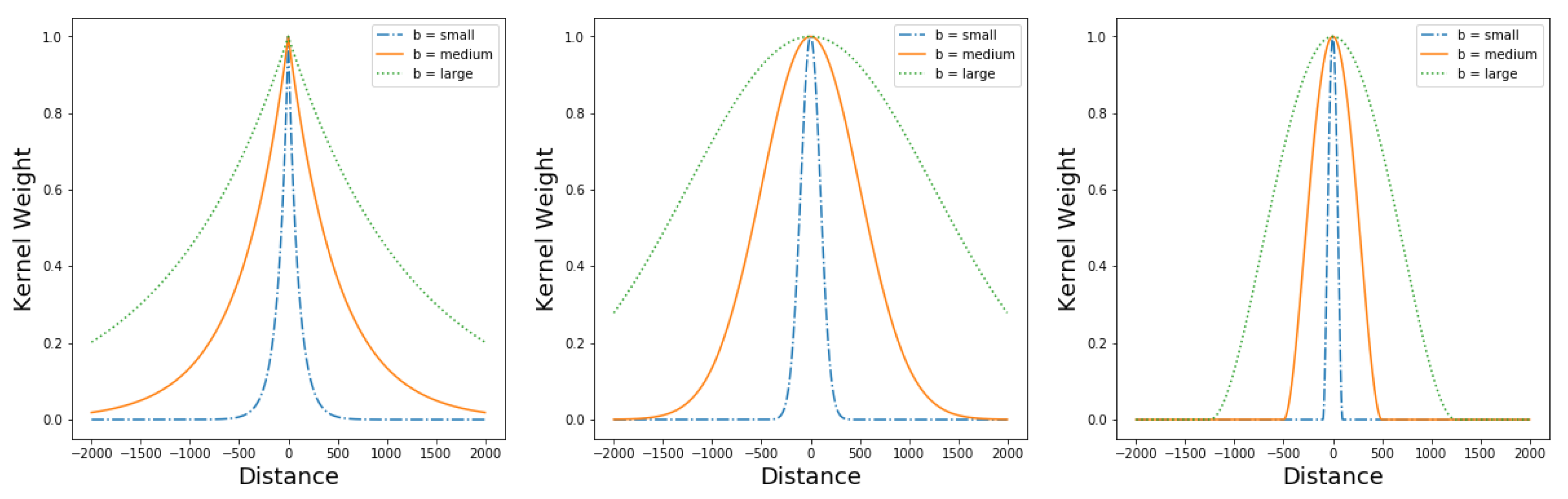
3.1.1. Kernel Functions

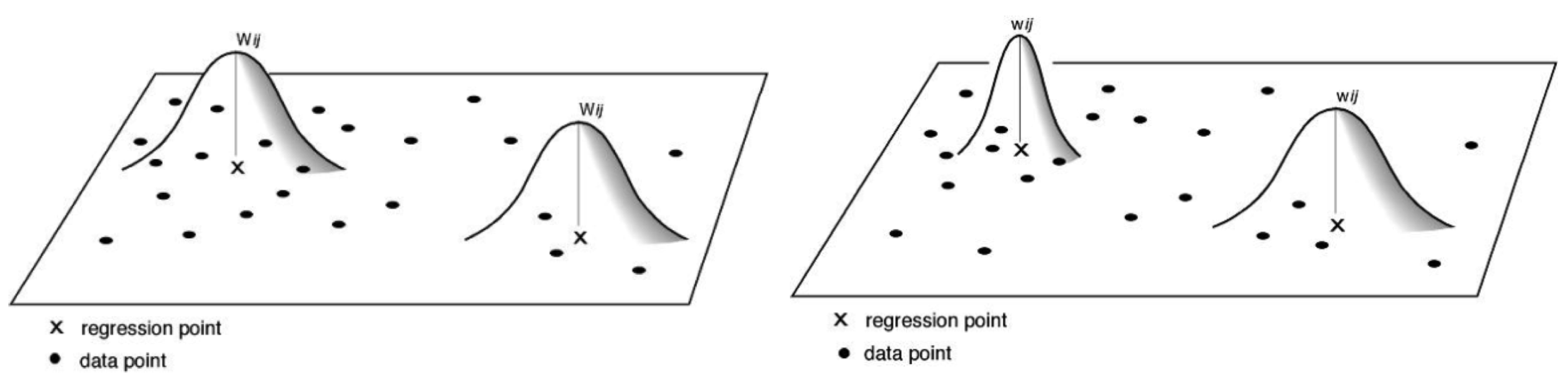
To calculate the weights matrix, a kernel function is applied to the distances between observations and calibration points. This kernel places more emphasis on observations that are closer than those farther away. The mgwr package offers the three most widely used kernel functions, which are the Gaussian, exponential, and bi-square functions as shown in

Table 3. Different kernel functions available to weight observations.

Function	Specification	Input Parameter
Gaussian	$w_{ij}=exp(-\frac{1}{2}{(\frac{d_{ij}}{b})}^2)$	kernel=‘gaussian’
Exponential	$w_{ij}=exp(-(\frac{|d_{ij}|}{b}))$	kernel=‘exponential’
Bi-square	$w_{ij}=\left\{\begin{array}{cc}{(1-{(d_{ij}/b)}^2)}^2\hfill & \mathrm{if} |d_{ij}|<b\hfill \\ 0\hfill & \mathrm{otherwise}\hfill \end{array}\right.$	kernel=‘bisquare’

. A potential issue with the Gaussian and exponential kernel functions is that all observations retain non-zero weight, regardless of how far they are from the calibration location. This means that even faraway observations can remain influential for moderate-to-large bandwidth parameters (Figure 3). As a result, the default behavior in mgwr is to use a bi-square kernel because it avoids this issue and has an intuitive interpretation: the bandwidth parameter is the distance or number of nearest neighbors away in space that the remaining observations have no influence. The bottom plot in Figure 3 demonstrates that for the bi-square kernel, even large bandwidths will result in observations that are weighted to exactly zero. Nevertheless, the kernel can be changed to either a Gaussian or an exponential function by altering the kernel input parameter where the option is available (see Table 3).

3.1.2. Kernel Types

Two types of kernel function are available in mgwr: fixed and adaptive. The former fixes the bandwidth parameter so that for each calibration location, the data are weighted with the same intensity, whereby this intensity is characterized by a measure of distance from the calibration location. A limitation of fixed-bandwidth kernels is that there can be calibration issues when there are sparsely-populated regions of a study area. The latter kernel type, known as an adaptive bandwidth kernel, avoids this issue. A nearest-neighbor definition of bandwidth ensures that the same number of observations are available for each local regression since the distance that spans the nearest-neighbors adapts from location to location. The difference between these two kernel types is illustrated in Figure 4. The fixed kernels (top) are the same regardless of the distribution of the data while the adaptive kernels (bottom) vary in shape depending upon the spatial distribution of the data. As a result, an adaptive bandwidth kernel is able to better handle irregularly shaped study areas, non-uniform spatial distributions of observations and edge effects and is therefore the default behavior in mgwr. In the event that a fixed bandwidth kernel is desired, it can be selected by setting fixed = True where it is available.

3.2. Bandwidth Selection

Bandwidth selection is carried out either by optimizing a model fit criterion or by manual specification. Optimal selection is preferred when there is no theoretical guide to manually specify the bandwidth. In this case, the Sel_BW class provides the functionality to apply different optimization routines and model fit criterion. First, an instance of the Sel_BW class is instantiated by passing the model inputs, $\mathit{X}$, $\mathit{y}$, and the geographic coordinates $(\mathit{u},\mathit{v})$. In this case, for both the Georgia and Berlin examples, the options are left to their default values, which implies an adaptive nearest-neighbor bi-square kernel using projected coordinates (i.e., Euclidian distances). The available kernel options were already discussed and spherical coordinates such as (longitude, latitude) can be accommodated by setting spherical = True. In addition, a full list of the available options for the Sel_BW functionality is available via the class docstrings. Next, the search method is called on the Sel_BW object that was instantiated. The search method controls the optimization method and model fit criterion. The default settings specify the use of a golden section search optimization routine and a corrected Akaike information criterion (AICc) as the model fit criterion. An equal interval search optimization routine can alternatively be selected by setting search_method = ‘interval’ and setting the interval option to the desired sampling interval. The available model fit criteria are illustrated in

Table 4. Different model fit criterion.

Name	Input Parameter
Cross-validation (CV)	criterion=‘CV’
Akaike information criterion (AIC)	criterion = ‘AIC’
Corrected AIC (AICc)	criterion = ‘AICc’
Bayesian information criterion (BIC)	criterion = ‘BIC’

; however an AICc is suggested because it penalizes smaller bandwidths that result in more complex models that consume more degrees of freedom. Following [2] a GWR-specific AICc takes the following form:

$$AI{C}_c=2n{log}_e\left(\frac{RSS}{n}\right)+n{log}_e\left(2\pi \right)+n\left\{\frac{n+tr\left(\mathit{S}\right)}{n-2-tr\left(\mathit{S}\right)}\right\},$$

(3)

where n is the number of observations, $\mathit{S}$ is the influence or hat matrix, and $RSS$ is the residual sum of squares.

#Examples of optimal bandwidth~selection

#Instantiate bandwidth selection object

>>> selector = Sel_BW(g_coords, g_y, g_X)

#Default golden section search using AICc criterion

>>> bw = selector.search()

>>> print(bw)

117.0

#Interval search using AICc criterion

>>> bw = selector.search(search_method = ‘interval’,

               interval = 2,

               bw_min = 101,

               bw_max = 150)

>>> print(bw)

117

3.3. Model Calibration

Model calibration is carried out by first instantiating a GWR model object. Then, the fit method for the GWR object is called to fit the model. An important input that must be specified for GWR calibration is the bandwidth parameter, which can be chosen via the optimal bandwidth selection routine discussed above.

#Calibrate a GWR model for Georgia dataset using computationally selected~bandwidth

>>> gwr_selector = Sel_BW(g_coords, g_y, g_X)

>>> gwr_bw = gwr_selector.search()

>>> print(gwr_bw)

117.0

>>> gwr_model = GWR(g_coords, g_y, g_X, gwr_bw)

>>> gwr_results = gwr_model.fit()

>>> print(gwr_results.resid_ss)

1650.85969828

The bandwidth can also be selected manually when there is a strong theoretical grounding or to explore potential spatial heterogeneity. Figure 5 displays the different patterns that arise for the percent rural parameter estimate surface when the bandwidth is varied from 25 to 150 nearest neighbors.

#Calibrate a GWR model for the Georgia dataset

#using a manually set~bandwidth

>>> gwr_model = GWR(g_coords, g_y, g_X, 117)

>>> gwr_results = gwr_model.fit()

>>> print(gwr_results.resid_ss)

1650.85969828

#Exploring spatial heterogeneity by manually varying~bandwidth

>>> fig, ax = plt.subplots(2, 3, figsize = (10, 6))

>>> bws = (x for x in range(25, 175, 25))

>>> vmins = []

>>> vmaxs = []

>>> for row in range(2):

     for col in range(3):

        bw = next(bws)

        gwr_model = GWR(g_coords, g_y, g_X, bw)

        gwr_results = gwr_model.fit()

        georgia[‘rural’] = gwr_results.params[:, -1]

        georgia.plot(‘rural’, ax = ax[row, col])

        ax[row,col].set_title(‘Bandwidth: ’ + str(bw))

        ax[row,col].get_xaxis().set_visible(False)

        ax[row,col].get_yaxis().set_visible(False)

        vmins.append(georgia[‘rural’].min())

        vmaxs.append(georgia[‘rural’].max())

>>> sm = plt.cm.ScalarMappable(norm=plt.Normalize(vmin=min(vmins), vmax=max(vmaxs)))

>>> fig.tight_layout()

>>> fig.subplots_adjust(right=0.9)

>>> cax = fig.add_axes([0.92, 0.14, 0.03, 0.75])

>>> sm._A = []

>>> cbar = fig.colorbar(sm, cax=cax)

>>> cbar.ax.tick_params(labelsize=10)

>>> plt.savefig(‘explore’)

>>> plt.show()

3.4. Probability Models

Though the examples in this paper will focus on calibrating Gaussian GWR models for continuous data, it is also possible to calibrate a Poisson GWR for count data or a Binomial logistic GWR for boolean data. To do so, the appropriate family object should be imported from the spglm package:

from spglm.family import Poisson, Binomial

and then it is necessary to set family = Poisson() or family = Binomial() when instantiating a Sel_BW or GWR object. Generally, it is not necessary to import or specify a Gaussian family object since it is the default behavior across mgwr.

3.5. Model Diagnostics

Once a GWR model calibration is complete, several diagnostic tools and statistics are available.

3.5.1. Model Fit

Model fit can be assessed using global statistics such as the AIC, AICc, or, a pseudo-$R^2$, which are all available as attributes of the GWRResults object that is returned from a successful model calibration. It is also possible to assess the fit of the model at each calibration location by mapping a local $R^2$ statistic. This local measure of fit provides an indication of how well the model fits over the smoothed data, focused at each site. Figure 6 shows that the individual regression models that comprise the GWR model have model fits that are both larger and smaller than the global $R^2$. It is also clear that the variation in model fit is spatially patterned with higher model fit in the north than in the south.

#Global model~fit

>>> gwr_selector = Sel_BW(g_coords, g_y, g_X)

>>> gwr_bw = gwr_selector.search()

>>> print(gwr_bw)

117.0

>>> gwr_model = GWR(g_coords, g_y, g_X, gwr_bw)

>>> gwr_results = gwr_model.fit()

>>> print(gwr_results.aic)

848.915407053

>>> print(gwr_results.aicc)

851.350292784

>>> print(gwr_results.R2)

0.678074266959

#Local model fit

>>> georgia[‘R2’] = gwr_results.localR2

>>> georgia.plot(‘R2’, legend = True)

>>> ax = plt.gca()

>>> ax.get_xaxis().set_visible(False)

>>> ax.get_yaxis().set_visible(False)

>>> plt.savefig(’local_R2’)

>>> plt.show()

3.5.2. Inference on Individual Parameter Estimates

Since GWR is an extension of the traditional regression framework, traditional inferential tools are available. A t-test can be carried out for each parameter, j, at each calibration location, i, where local t-values are given by:

$$t_{(i,j)}=\frac{{\widehat{\beta }}_{(i,j)}}{s{e}_{(i,j)}},$$

(4)

where $s{e}_{(i,j)}$ is the standard error associated with the $i{j}^{th}$ parameter estimate. However, the nature of the distance-weighting scheme can potentially cause the local sub-samples to be dependent and a correction to account for multiple dependent hypothesis tests has been developed [12]. Instead of employing the typical $\alpha =0.05$ value that pertains to a $95\%$ confidence interval, an alternative corrected $\alpha$ is given by:

$$\alpha =\frac{\xi }{\frac{ENP}{p}},$$

(5)

where $ENP$ is the effective number of parameters obtained by taking the trace of the GWR hat matrix (denoted by $\mathit{S}$), p is the number of explanatory variables, and $\xi$ is the desired type I error rate across the set of tests. The ratio $\frac{ENP}{p}$ ($ENP>p$) is representative of the number of multiple tests and if $p_e=p$ then $\xi =\alpha$ and the number of tests performed by GWR and a global regression are equivalent.

The adj_alpha and filter_t methods are available to compute the corrected alpha and filter out parameters whose confidence intervals overlap with zero (i.e., statistically insignificant). Applying the correction typically results in more conservative hypothesis tests that lead to the null hypothesis $\widehat{{\beta }_i}=0$ being accepted more often. This is demonstrated in Figure 7 where the right panel that uses the correction displays statistically significant parameter estimates (i.e., those not shaded gray), than the middle panel that does not use the correction for the foreign born parameter estimates of the Georgia dataset.Therefore, the default behavior of the filter_t method is to automatically use the correction defined in Equation (5) with $\xi$ = 0.05.

#Visualizing hypothesis tests for significance of parameter estimates

>>> gwr_selector = Sel_BW(g_coords, g_y, g_X)

>>> gwr_bw = gwr_selector.search()

>>> print(gwr_bw)

117.0

>>> gwr_model = GWR(g_coords, g_y, g_X, gwr_bw)

>>> gwr_results = gwr_model.fit()

#default behavior using corrected alpha

>>> filter_tc = gwr_results.filter_tvals()

#without correction using common alpha

>>> filter_t = gwr_results.filter_tvals(alpha = 0.05)

>>> georgia[‘fb’] = gwr_results.params[:, 1]

>>> georgia[‘fb_t’] = filter_t[:, 1]

>>> georgia[‘fb_tc’] = filter_tc[:, 1]

>>> fig, ax = plt.subplots(1, 3, figsize = (12, 3))

>>> georgia.plot(‘fb’,

               **{‘edgecolor’: ‘black’,

               ‘alpha’: .65,

               ‘linewidth’: .5},

            ax = ax[0],

            legend=True)

>>> ax[0].get_xaxis().set_visible(False)

>>> ax[0].get_yaxis().set_visible(False)

>>> ax[0].set_title(’Parameter estimates’)

>>> georgia.plot(‘fb’,

               **{‘edgecolor’: ‘black’,

               ‘alpha’: .65,

               ‘linewidth’: .5},

            ax = ax[1],

            legend=True)

>>> georgia[filter_t[:, 1] == 0].plot(color = ‘grey’,

                              ax = ax[1],

                              **{‘edgecolor’: ’black’,

                                ‘linewidth’: .5})

>>> ax[1].get_xaxis().set_visible(False)

>>> ax[1].get_yaxis().set_visible(False)

>>> ax[1].set_title(’Composite’)

>>> georgia.plot(‘fb’,

               **{‘edgecolor’: ‘black’,

               ‘alpha’: .65,

               ‘linewidth’: .5},

            ax = ax[2],

            legend=True)

>>> georgia[filter_tc[:, 1] == 0].plot(color = ‘grey’,

                               ax = ax[2],

                               **{‘edgecolor’: ’black’,

                                 ‘linewidth’: .5})

>>> ax[2].get_xaxis().set_visible(False)

>>> ax[2].get_yaxis().set_visible(False)

>>> ax[2].set_title(‘Composite with correction’)

plt.savefig(‘testing’)

plt.show()

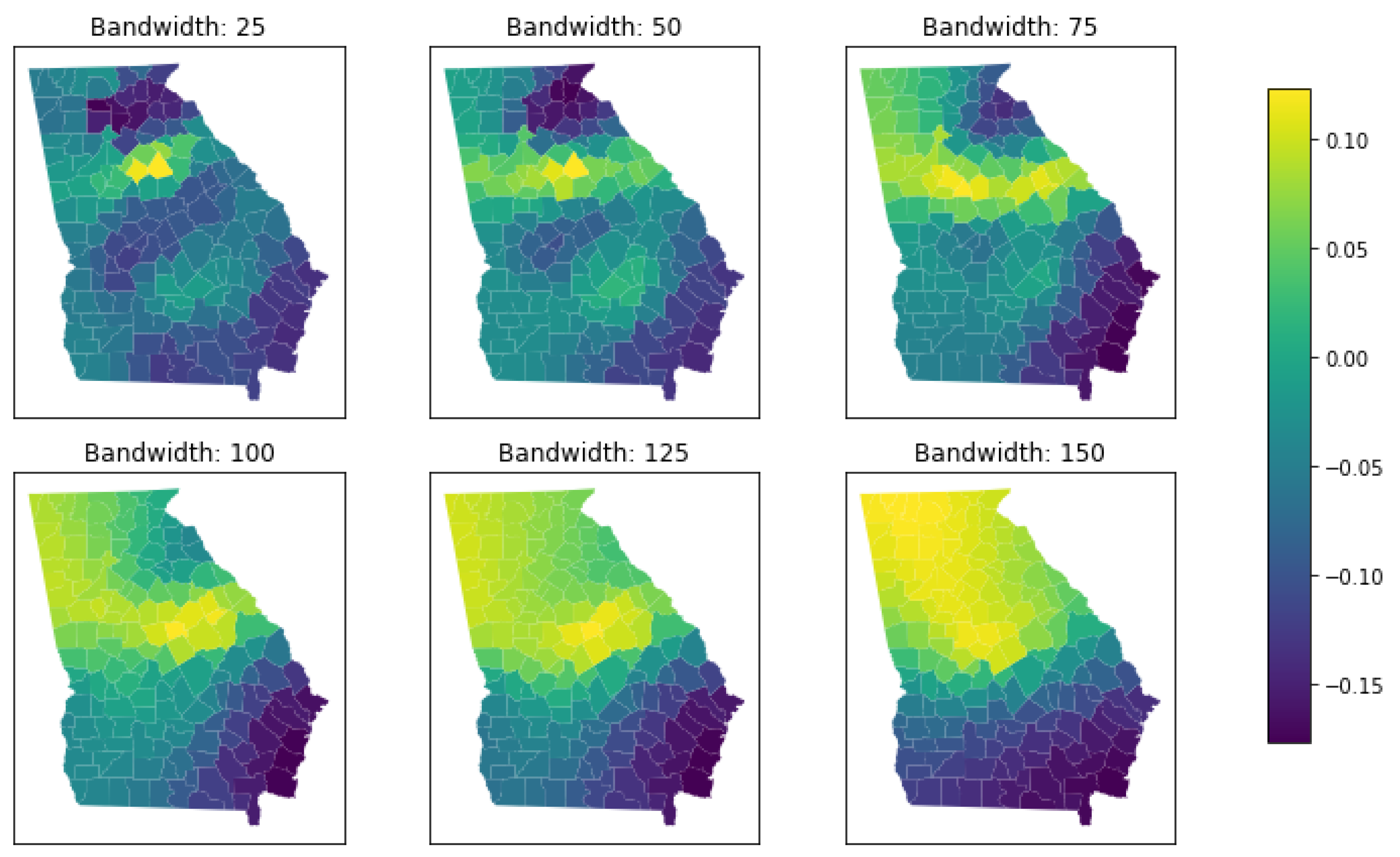
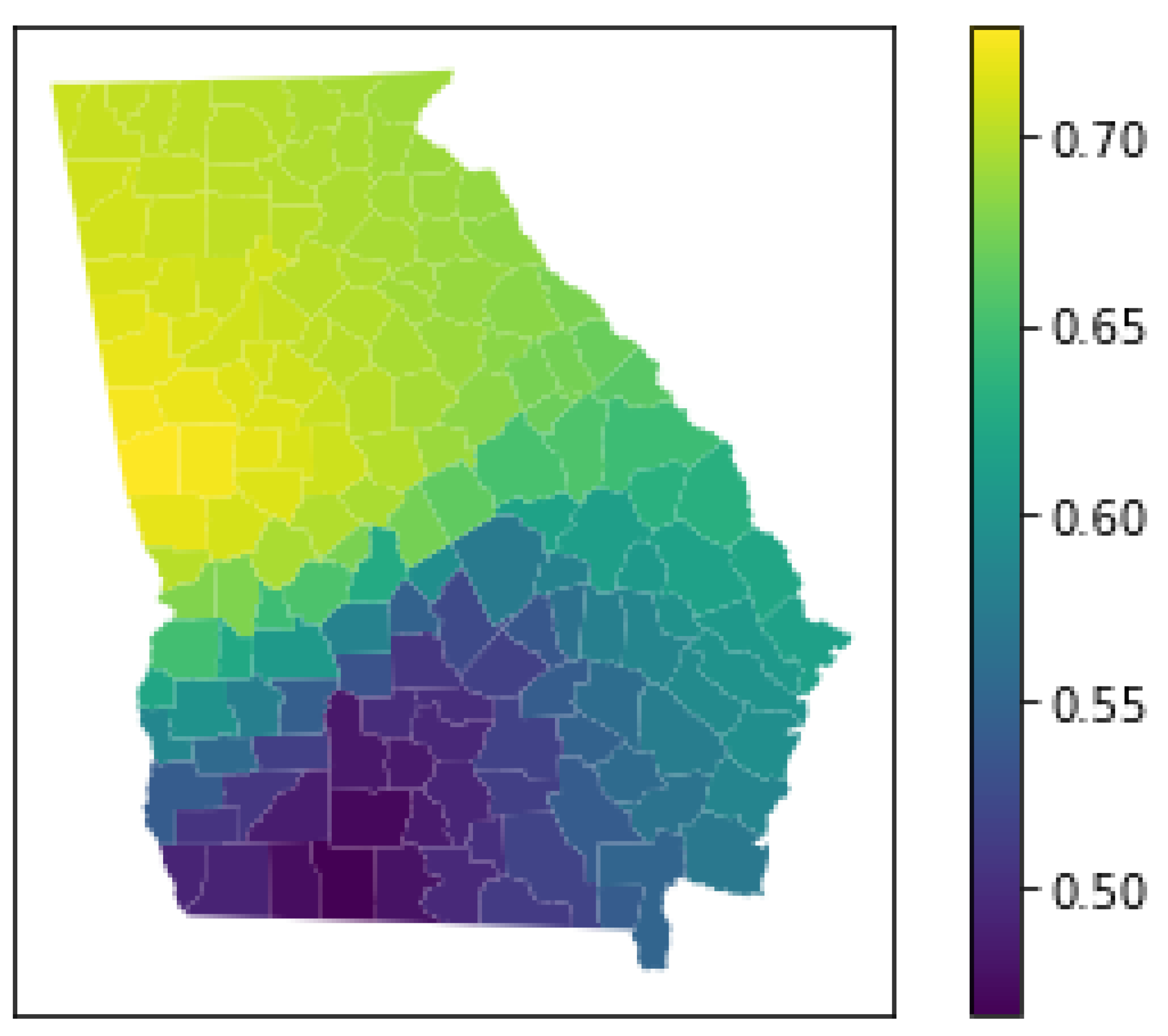
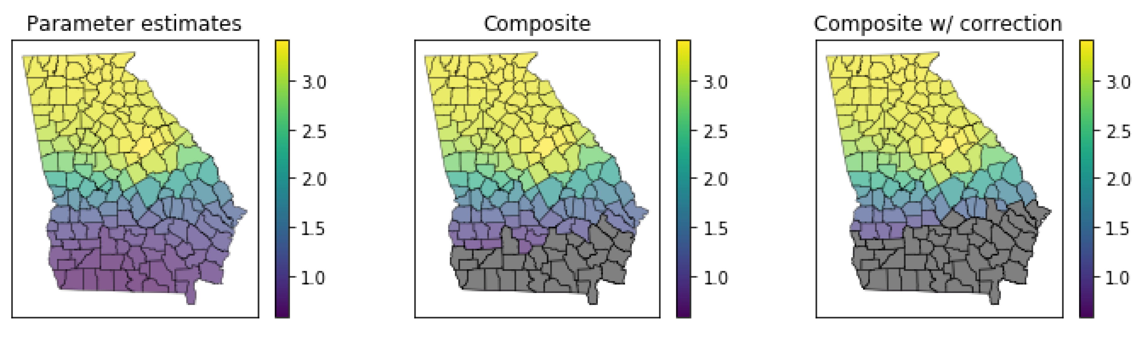
3.5.3. Inference on Surface of Parameter Estimates

It is also possible to test the statistical significance of each surface of parameter estimates produced by GWR via Monte Carlo methods. The spatial variability test shuffles the observations in space, re-calibrates GWR on the randomized data while holding the model specification constant, and then computes the variability of the resulting parameter estimates for each surface. This process is repeated and the number of times that the variability of each surface from the randomized data is higher than the variability of each original surface is used to construct pseudo p-values for hypothesis testing. A pseudo-p-value smaller than 0.05 indicates that the observed spatial variability of a coefficient surface is significant at the 95% confidence level (i.e., non-random).

One issue with the test for spatial variability is that it requires GWR to be calibrated many times, which is computationally expensive. It may even be computationally prohibitive to use the test for larger datasets and users should exercise caution in how many replications they specify for the test, keeping in mind that the default number of iterations is 1000. In the example below, the four p-values produced correspond to parameter estimate surfaces for the intercept, the foreign born variable, the African American variable, and the rural variable. For a GWR model with a bandwidth of 50 and repetitions of 100, 1000 or 2000, the p-value for the intercept and the rural variable are larger than 0.05 and indicate the parameter estimates surfaces exhibit no significant local variation, whereas the p-values for foreign born and African Americans are smaller than 0.05 and indicate the parameter estimates surfaces do exhibit significant local variation.

#Visualizing hypothesis tests for significance of parameter~estimates

#Manually set bandwidth to 50 and fit

>>> gwr_model = GWR(g_coords, g_y, g_X, 50)

>>> gwr_results = gwr_model.fit()

#100 iterations

>>> p_vals_100 = gwr_results.spatial_variability(gwr_selector, 100)

>>> print(p_vals_100)

[ 0.153  0.019  0.026  0.155]

#default is 1000 iterations

>>> p_vals_1000 = gwr_results.spatial_variability(gwr_selector)

>>> print(p_vals_1000)

[ 0.12  0.03  0.04  0.14]

#2000 iterations

>>> p_vals_2000 = gwr_results.spatial_variability(gwr_selector, 2000)

>>> print(p_vals_2000)

[ 0.1515  0.0195  0.023   0.146 ]

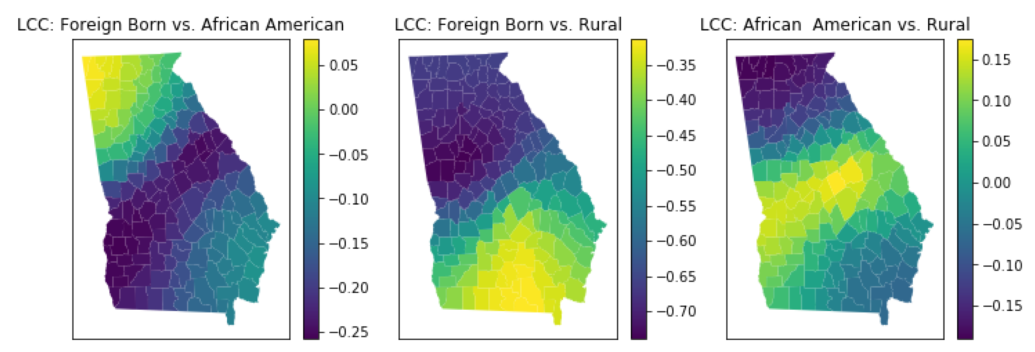
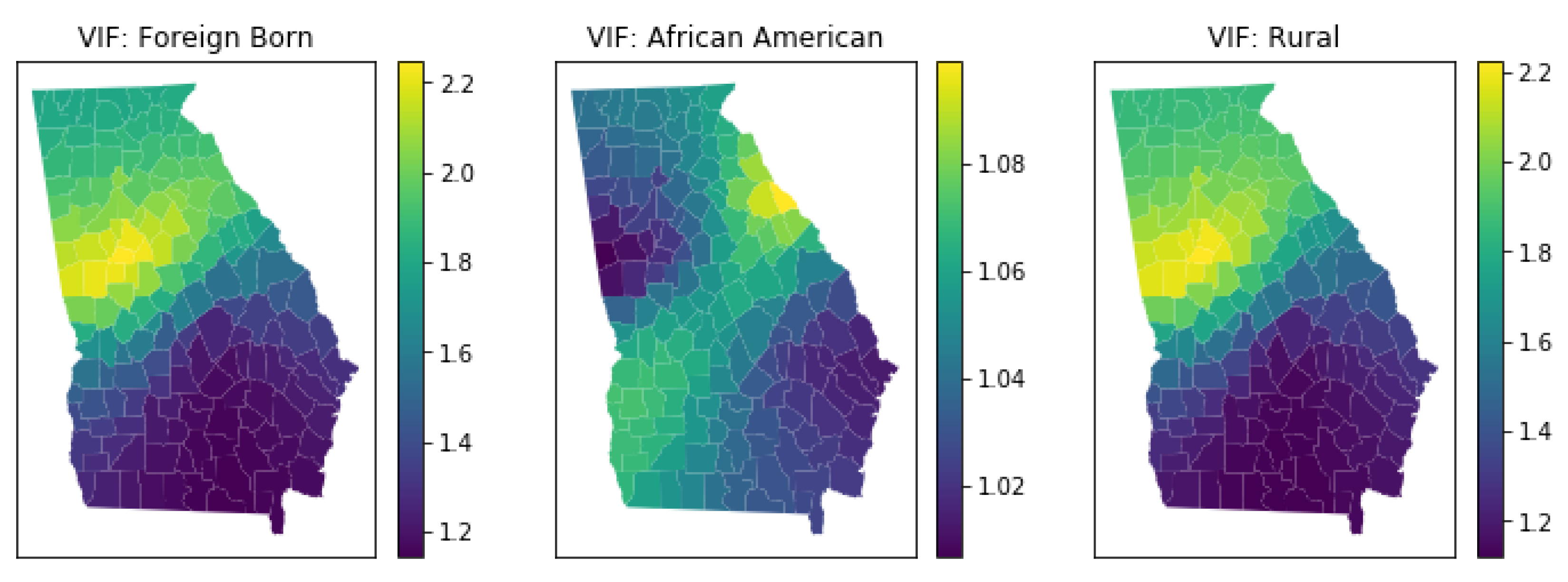
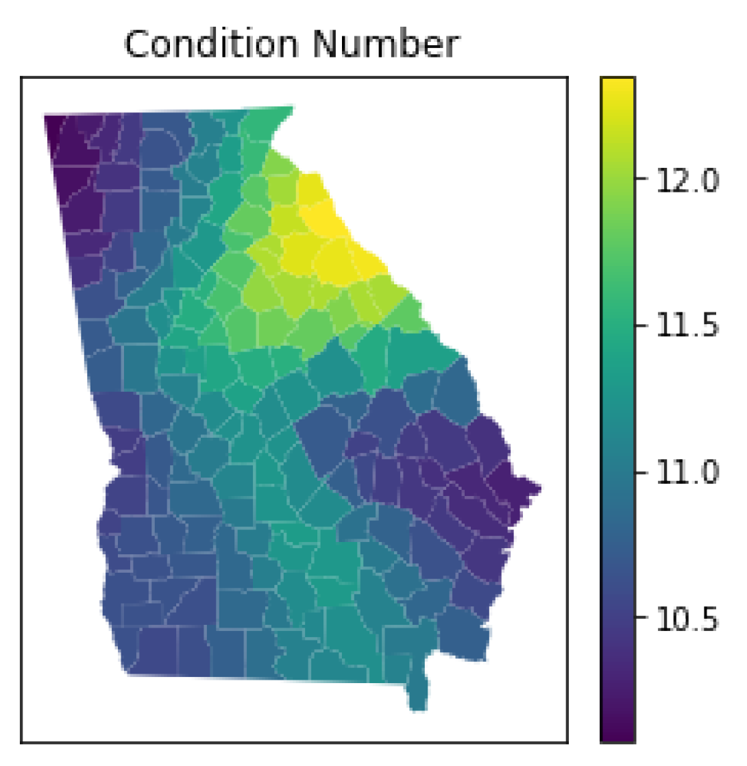
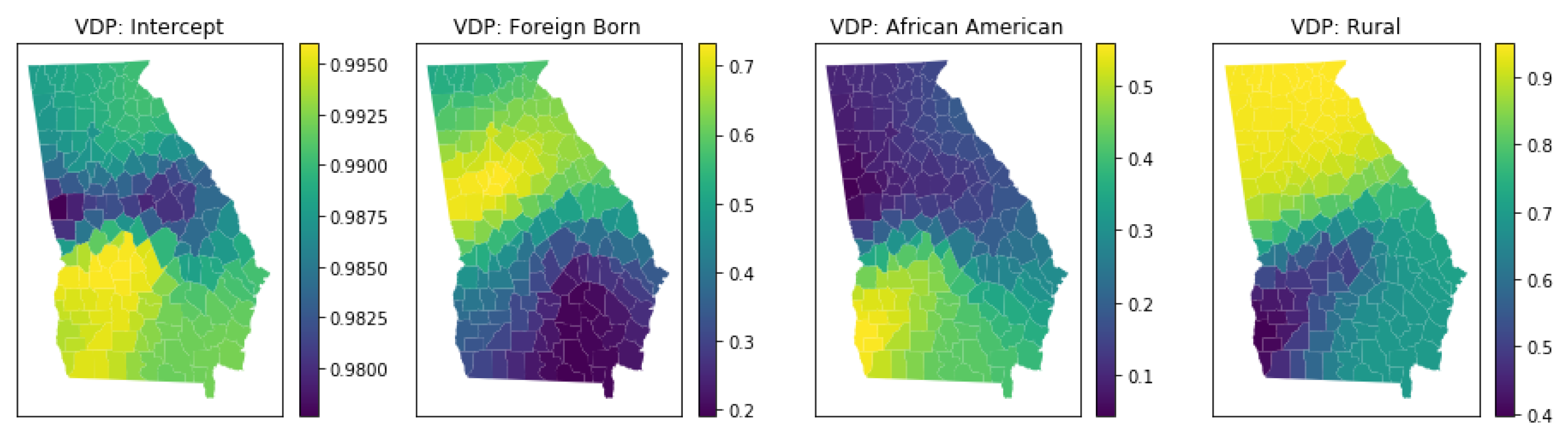
3.5.4. Local Multicollinearity

Though there are many tools available to evaluate multicollinearity amongst explanatory variables for traditional regression models, some extra care is needed for local models that borrow data from nearby locations. Within each local model, there may be higher levels of collinearity than is present in the dataset as a whole [13]. Higher levels of collinearity are associated with problems such as estimate instability, unintuitive parameter signs, high $R^2$ diagnostics despite few or no significant parameters, and inflated standard errors for parameter estimates [14,15]. As a result, diagnostic tools have been designed to detect levels of local multicollinearity, including local correlation coefficients (CC), local variation inflation factors (VIF), local condition number (CN), and local variation decomposition proportions (VDP) [13,16].

Each local measure has a rule of thumb that indicates that there might be an issue due to multicollinearity: CC higher than 0.8; VIF higher than 10; CN higher than 30: VDP higher than 0.5 each indicate multicollinearity in some measure. However, these rules are not absolute and obtaining lower values does not mean collinearity is innocuous, nor does obtaining larger values guarantee collinearity is indeed problematic. In addition, local CC’s and local VIF’s do not consider the local intercept term, while the local CN is a single aggregate measure for all of the variables rather than producing an individual measure for each variable. Figure 8, Figure 9, Figure 10 and Figure 11 demonstrate maps of local CC’s, local VIF’s, local CN’s, and local VDP’s, respectively, for the Georgia example using an AICc optimized bandwidth. The VDP’s indicate that some areas may be subject to the effects of collinearity; however, none of the CC’s, VIF’s nor CN’s indicate that collinearity is problematic for any of the calibration locations. In addition, it has been demonstrated that multicollinearity is not inherently more problematic in GWR [17] than a traditional regression and some of the patterns theorized to be associated with multicollinearity may be indicative [18] of reality or due to scale misspecification [19].

>>> gwr_selector = Sel_BW(g_coords, g_y, g_X)

>>> gwr_bw = gwr_selector.search()

>>> print(gwr_bw)

117.0

>>> gwr_model = GWR(g_coords, g_y, g_X, gwr_bw)

>>> gwr_results = gwr_model.fit()

>>> LCC, VIF, CN, VDP = gwr_results.local_collinearity()

>>> names = [‘Foreign Born vs. African American’,

          ‘Foreign Born vs. Rural’,

          ‘African  American vs. Rural’]

>>> fig, ax = plt.subplots(1, 3, figsize = (12, 4))

>>> for col in range(3):

   georgia[‘vif’] = LCC[:, col]

   georgia.plot(‘vif’, ax = ax[col], legend = True)

   ax[col].set_title(‘LCC: ’ + names[col])

   ax[col].get_xaxis().set_visible(False)

   ax[col].get_yaxis().set_visible(False)

>>> names = [‘Foreign Born’, ‘African American’, ‘Rural’]

>>> fig, ax = plt.subplots(1, 3, figsize = (12, 4))

>>> for col in range(3):

   georgia[‘vif’] = VIF[:, col]

   georgia.plot(‘vif’, ax = ax[col], legend = True)

   ax[col].set_title(‘VIF: ’ + names[col])

   ax[col].get_xaxis().set_visible(False)

   ax[col].get_yaxis().set_visible(False)

>>> fig, ax = plt.subplots(1, 1, figsize = (4, 4))

>>> georgia[‘cn’] = CN

>>> georgia.plot(‘cn’, legend = True, ax = ax)

>>> ax.set_title(‘Condition Number’)

>>> ax.get_xaxis().set_visible(False)

>>> ax.get_yaxis().set_visible(False)

>>> names = [‘Intercept’, ‘Foreign Born’, ‘African American’, ‘Rural’]

>>> fig, ax = plt.subplots(1, 4, figsize = (16, 4))

>>> for col in range(4):

   georgia[‘vdp’] = VDP[:, col]

   georgia.plot(‘vdp’, ax = ax[col], legend = True)

   ax[col].set_title(‘VDP: ’ + names[col])

   ax[col].get_xaxis().set_visible(False)

   ax[col].get_yaxis().set_visible(False)

3.6. Out-of-Sample Spatial Prediction

Though the primary focus of mgwr is on inference, it is also possible to use GWR as a tool for out-of-sample spatial prediction in a manner similar to interpolation methods [20]. For example, it is feasible to first calibrate a GWR model using data where both the dependent and independent variables are observed in order to obtain an AIC optimized bandwidth. Out-of-sample predictions are then obtained by borrowing exogenous data at the unobserved locations from surrounding sites based on the the previously estimated bandwidth, estimating the parameters for the prediction site, and then calculating predicted values of the dependent variable using the borrowed explanatory covariates and estimates. This is demonstrated below by splitting the Georgia dataset into a calibration dataset for obtaining a bandwidth and holding out some observations to then predict.

# Out-of-sample prediction using~GWR

#Split data into calibration and prediction sets

>>> np.random.seed(908)

>>> sample = np.random.choice(range(159), 10)

>>> mask = np.ones_like(g_y, dtype = bool).flatten()

>>> mask[sample] = False

>>> cal_coords = np.array(g_coords)[mask]

>>> cal_y = g_y[mask]

>>> cal_X = g_X[mask]

>>> pred_coords = np.array(g_coords)[~mask]

>>> pred_y = g_y[~mask]

>>> pred_X = g_X[~mask]

#Calibrate GWR model

>>> gwr_selector = Sel_BW(cal_coords, cal_y, cal_X)

>>> gwr_bw = gwr_selector.search(bw_min = 2)

>>> print(gwr_bw)

109.0

>>> model = GWR(cal_coords, cal_y, cal_X, gwr_bw)

>>> gwr_results = model.fit()

#Make predictions

>>> pred_results = model.predict(pred_coords, pred_X)

#Check correlation between known and predicted values

>>> corr = np.corrcoef(pred_results.predictions.flatten(),

                 pred_y.flatten())[0][1]

print(corr)

0.914249268428

4. MGWR Functionality

So far, all the concepts and examples discussed in this paper have assumed that the data-borrowing range (i.e., bandwidth), or process scale is the same for each relationship in a given model. Any time that there are multiple distinct spatial scales generating data and GWR is applied, one or more of the scales are misspecified, which can result in biased parameter estimates. A more intuitive assumption is that each relationship may occur at a different scale. MGWR provides an extension that allows each variable to be associated with a distinct bandwidth by recasting GWR as a generalized additive model (GAM) such that:

$$y=\sum _{j=1}^k{f}_j+ϵ,$$

(6)

where $f_j$ is a smoothing function (i.e., data-borrowing scheme) applied to the $j^{th}$ explanatory variable that may may be characterized by distinct bandwidth parameter [3]. In this section, concepts and novel functionality necessary to calibrate and assess an MGWR model are introduced with special attention to details that differ from the GWR functionality previously introduced.

4.1. Standardizing the Variables

In order to compare each of the bandwidths obtained from an MGWR model, it is necessary to standardize the dependent and independent variables so that they are centered at zero and based on the same range of variation. Otherwise it may be difficult to objectively compare the estimated bandwidths because it is possible that they are also representative of the scale and variation of the independent variables [3].

#Standardize~variables

#Georgia dataset

>>> g_X = (g_X - g_X.mean(axis = 0)) / g_X.std(axis = 0)

>>> g_y = (g_y - g_y.mean(axis = 0)) / g_y.std(axis = 0)

#Standardize Berlin dataset

>>> b_X = (b_X - b_X.mean(axis = 0)) / b_X.std(axis = 0)

>>> b_y = (b_y - b_y.mean(axis = 0)) / b_y.std(axis = 0)

4.2. Bandwidth Selection and Model Calibration

MGWR uses a back-fitting algorithm for model calibration, based on GAM fitting methods [3,7]. This involves sequentially calibrating a series of univariate GWR models based on the partial residuals from the previous iteration until the MGWR model converges to a solution. Two primary differences arise in how an MGWR model is specified and calibrated in mgwr when compared to GWR. First, though it is possible to utilize a GWR object without carrying out computational bandwidth selection, the same is not true of MGWR because bandwidth selection and parameter estimation are inherently linked. Instead, a Sel_BW object must be passed to an MGWR object in order to carry out MGWR calibration, which is demonstrated below:

#Example of MGWR calibration (Berlin data)

>>> mgwr_selector = Sel_BW(b_coords, b_y, b_X, multi = True)

>>> mgwr_bw = mgwr_selector.search()

>>> print(mgwr_bw)

[191.0, 1279.0, 79.0, 2200.0]

>>> mgwr_results = MGWR(b_coords, b_y, b_X, mgwr_selector).fit()

A Sel_BW object is necessary for obtaining model results because parameter estimation occurs simultaneously with bandwidth selection and therefore, much of the results from Sel_BW are needed for preparing the model output and computing MGWR model diagnostics. A second difference between MGWR and GWR is that the MGWR routine must be initialized with starting values of the parameters for each variable. Ref. [3] demonstrate how using the local parameter estimates from a calibrated GWR can speed up the MGWR calibration, rather than starting from zero or assuming a global bandwidth (i.e., using OLS results). As a result, this is the default behavior in mgwr.

4.3. Manually Setting Covariate-Specific Bandwidths

Though MGWR calibration requires the use of a Sel_BW object, it is still possible to manually select bandwidth parameters by setting both a minimum and maximum bandwidth to the same value using the multi_bw_min and multi_bw_max input options. A difference between these options and the bw_min and bw_max arguments used for GWR calibration is that the former must be specified using a list. If a list with a single value is specified, then this value is applied to all of the variables. However, it is also possible to specify a minimum and maximum bandwidth value for each variable in the model. Each of the these options is demonstrated below:

#Example of manual bandwidth selection in~MGWR

#Apply the same bandwidth to all variables

>>> mgwr_selector = Sel_BW(b_coords, b_y, b_X, multi = True)

>>> mgwr_bw = mgwr_selector.search(multi_bw_min = [500],

                         multi_bw_max = [500])

>>> print(mgwr_bw)

[500.0, 500.0, 500.0, 500.0]

>>> mgwr_results = MGWR(b_coords, b_y, b_X, mgwr_selector).fit()

#Unique manual bandwidths

>>> mgwr_selector = Sel_BW(b_coords, b_y, b_X, multi = True)

>>> mgwr_bw = mgwr_selector.search(multi_bw_min = [150, 500, 750, 1000],

                         multi_bw_max = [150, 500, 750, 1000])

>>> print(mgwr_bw)

[150.0, 500.0, 750.0, 1000.0]

>>> mgwr_results = MGWR(b_coords, b_y, b_X, mgwr_selector).fit()

4.4. Model Fit

Though it is possible to calculate an $R^2$ to assess model fit for MGWR, it is ideal to use a model fit criterion that better accounts for model complexity [2], such as the AICc introduced in Equation (3). Until recently, it was not possible to compute the AICc for MGWR because the back-fitting algorithm utilized for calibration did not produce a hat matrix (i.e., $\mathit{S}$ in Equation (3)). Previous software implementations that are able to calibrate (i.e., a particular parameterization of the psdm function in GWmodel), report an AICc value; however, this value is the minimum AICc obtained across the collection of the univariate GWR components that comprise the GAM used to calibrate MGWR [21]. In contrast, mgwr implements a new algorithm put forth by [7] that produces a hat matrix, allowing a proper AICc value that applies to the entire MGWR model to be computed according to Equation (3). This AICc model fit criterion for MGWR can be assessed in mgwr in a similar fashion to that of GWR using mgwr_results.aicc.

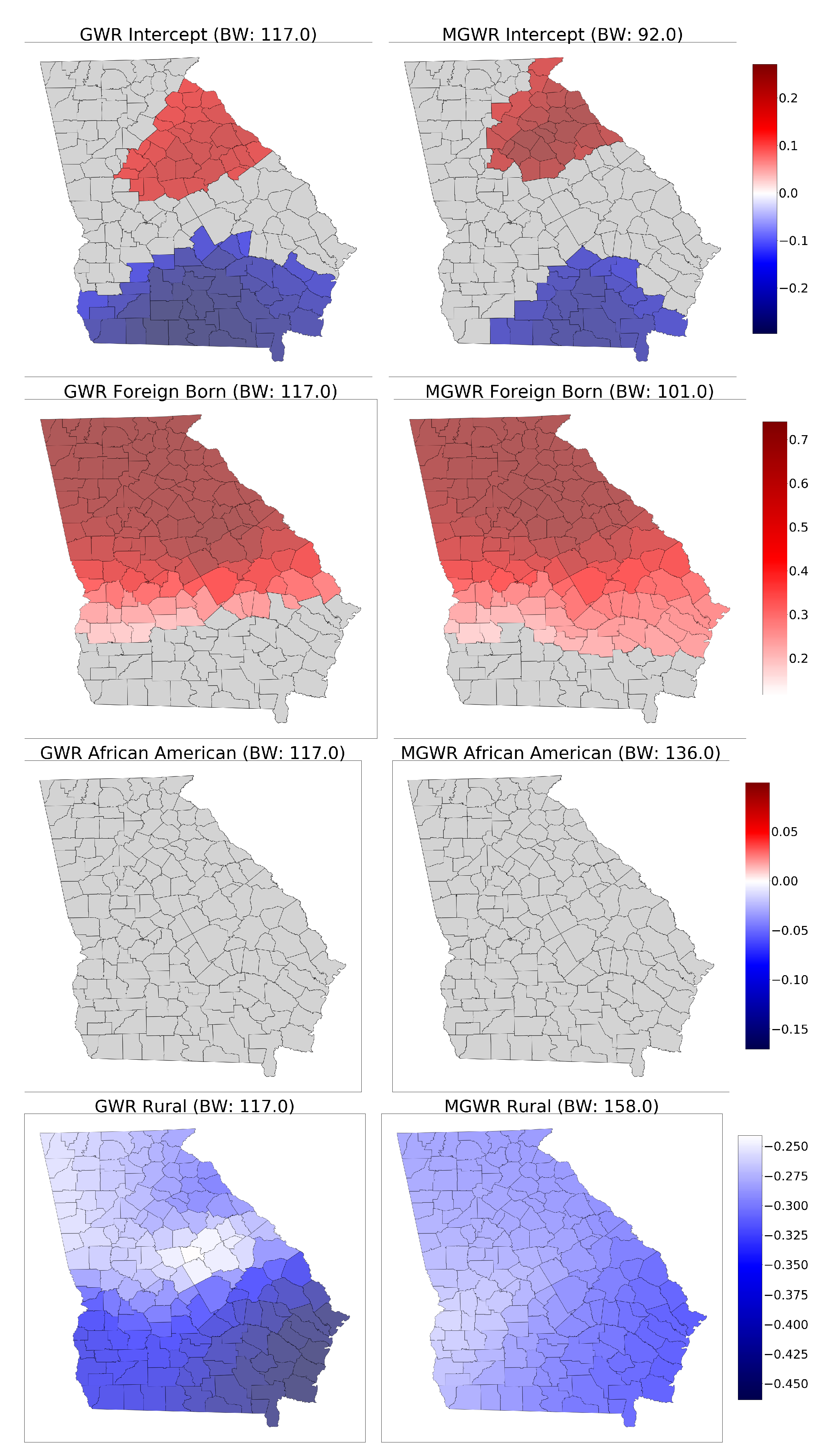
4.5. Inference on Parameter Estimates

As with GWR, it is necessary to apply the modified hypothesis testing framework described above. However, in the case of MGWR, it is possible to extend the testing framework to formulate a covariate-specific corrected hypothesis test for each surface of parameter estimates. This novel methodology is described in [7] and the necessary functionality is not currently available in other software implementations other than mgwr. In MGWR, the hat matrix, $\mathit{S}$, that maps the observed dependent variable onto the fitted values of the dependent variable, can be decomposed into covariate-specific contributions, ${\mathit{R}}_j$. With this, it is possible to compute a distinct measure of the effective number of parameters (ENP) for each parameter surface:

$$EN{P}_j=tr\left({\mathit{R}}_{\mathit{j}}\right)$$

(7)

Using the covariate-specific ENP’s, Equation (5) can be updated to:

$${\alpha }_j=\frac{{\xi }_m}{EN{P}_j},$$

(8)

where p drops out because for each relationship $p=1$. The default behavior in mgwr is to use ${\alpha }_j$ to compute a covariate-specific critical t-value for hypothesis testing. It is possible to inspect each $EN{P}_j$, ${\alpha }_j$, and the adjusted t-values as follows:

#First set up model

>>> mgwr_selector = Sel_BW(b_coords, b_y, b_X, multi = True)

>>> mgwr_bw = mgwr_selector.search()

>>> mgwr_results = MGWR(b_coords, b_y, b_X, mgwr_selector).fit()

#Covariate-specific ENP

>>> print(mgwr_results.ENP_j)

[31.89989861, 4.77588266, 73.79013919, 1.40343481]

#Covrariate-specific adjusted alpha at 95% CI

>>> print(mgwr_results.adj_alpha_j[:, 1])

[ 0.0015674   0.01046927  0.0006776   0.03562688]

#Covariate-specific adjusted critical t-value

>>> print(mgwr_results.critical_tval())

[ 3.16585816  2.56212889  3.40333525  2.10245302]

It is possible to use these values for inference with the filter_tvals method. By default filter_tvals returns an array of t-values where “insignificant” estimates are (at the $95\%$ significance level) set to zero.

>>> mgwr_filtered_t = mgwr_results.filter_tvals()

Then, it is possible to visualize only the coefficients associated with non-zero t-values. In addition, it is recommended to visualize the surfaces that result from MGWR in comparison to those from GWR to understand how surfaces vary under different assumptions about process scale. The compare_surfaces function is available specifically for comparative visualization between two surfaces and is demonstrated below in two examples of inference in MGWR.

4.5.1. The Georgia Dataset

The code below demonstrates inference using MGWR using the Georgia dataset (this example is available in more detail in Yu et al. [7]). Since the GWR bandwidth of 117.0 is relatively large and none of the MGWR bandwidths are small, there are only some minor differences between GWR and MGWR as displayed in Figure 12. For the intercept, Foreign Born, and African American, the patterns in the relationships for both the significant and insignificant parameter estimates are all very similar. This is due to the fact that for these surfaces, the MGWR bandwidths are all relatively similar in magnitude (i.e., +/− approximately 15 nearest-neighbors). In contrast, there is a larger difference in the pattern of the coefficients for the rural variable between GWR and MGWR and a larger difference between the bandwidths (i.e., 41 nearest neighbors). Nevertheless, the rural parameter estimate surfaces for both GWR and MGWR are still similar and both are composed of statistically significant negative estimates. Overall, these results show that when GWR and MGWR estimate similar bandwidths, the associated parameter estimates and hypothesis tests are also similar.

#Calibrate GWR using standardized~data

>>> gwr_selector = Sel_BW(g_coords, g_y, g_X)

>>> gwr_bw = gwr_selector.search()

print(gwr_bw)

117.0

>>> gwr_model = GWR(g_coords, g_y, g_X, gwr_bw)

>>> gwr_results = gwr_model.fit()

#Prepare GWR results for~mapping

#Add GWR parameters to GeoDataframe

>>> georgia[‘gwr_intercept’] = gwr_results.params[:, 0]

>>> georgia[‘gwr_fb’] = gwr_results.params[:, 1]

>>> georgia[‘gwr_aa’] = gwr_results.params[:, 2]

>>> georgia[‘gwr_rural’] = gwr_results.params[:, 3]

#Obtain t-vals filtered based on multiple testing correction

>>> gwr_filtered_t = gwr_results.filter_tvals()

#Calibrate MGWR~model

>>> mgwr_selector = Sel_BW(g_coords, g_y, g_X, multi = True)

>>> mgwr_bw = mgwr_selector.search(multi_bw_min = [2])

print(mgwr_bw)

[92.0, 101.0, 136.0, 158.0]

>>> mgwr_results = MGWR(g_coords, g_y, g_X, mgwr_selector).fit()

#Prepare MGWR results for~mapping

#Add MGWR parameters to GeoDataframe

>>> georgia[‘mgwr_intercept’] = mgwr_results.params[:, 0]

>>> georgia[‘mgwr_fb’] = mgwr_results.params[:, 1]

>>> georgia[‘mgwr_aa’] = mgwr_results.params[:, 2]

>>> georgia[‘mgwr_rural’] = mgwr_results.params[:, 3]

#Obtain t-vals filtered based on multiple testing correction

>>> mgwr_filtered_t = mgwr_results.filter_tvals()

>>> kwargs1 = {‘edgecolor’: ‘black’, ‘alpha’: .65}

>>> kwargs2 = {‘edgecolor’: ‘black’}

>>> compare_surfaces(georgia, ‘gwr_intercept’, ‘mgwr_intercept’,

                gwr_filtered_t[:, 0], gwr_bw, mgwr_filtered_t[:, 0],

                mgwr_bw[0], ‘Intercept’, kwargs1, kwargs2,

                savefig = ‘g1’)

>>> compare_surfaces(georgia, ‘gwr_fb’, ‘mgwr_fb’, gwr_filtered_t[:, 1],

                gwr_bw, mgwr_filtered_t[:, 1], mgwr_bw[1],

                ‘Foreign Born’, kwargs1, kwargs2, savefig = ‘g2’)

>>> compare_surfaces(georgia, ‘gwr_aa’, ‘mgwr_aa’, gwr_filtered_t[:, 2],

                gwr_bw, mgwr_filtered_t[:, 2], mgwr_bw[2],

                ‘African American’, kwargs1, kwargs2, savefig = ‘g3’)

>>> compare_surfaces(georgia, ‘gwr_rural’, ‘mgwr_rural’, gwr_filtered_t[:, 3],

                gwr_bw, mgwr_filtered_t[:, 3], mgwr_bw[3],

                ‘Rural’, kwargs1, kwargs2, savefig = ‘g4’)

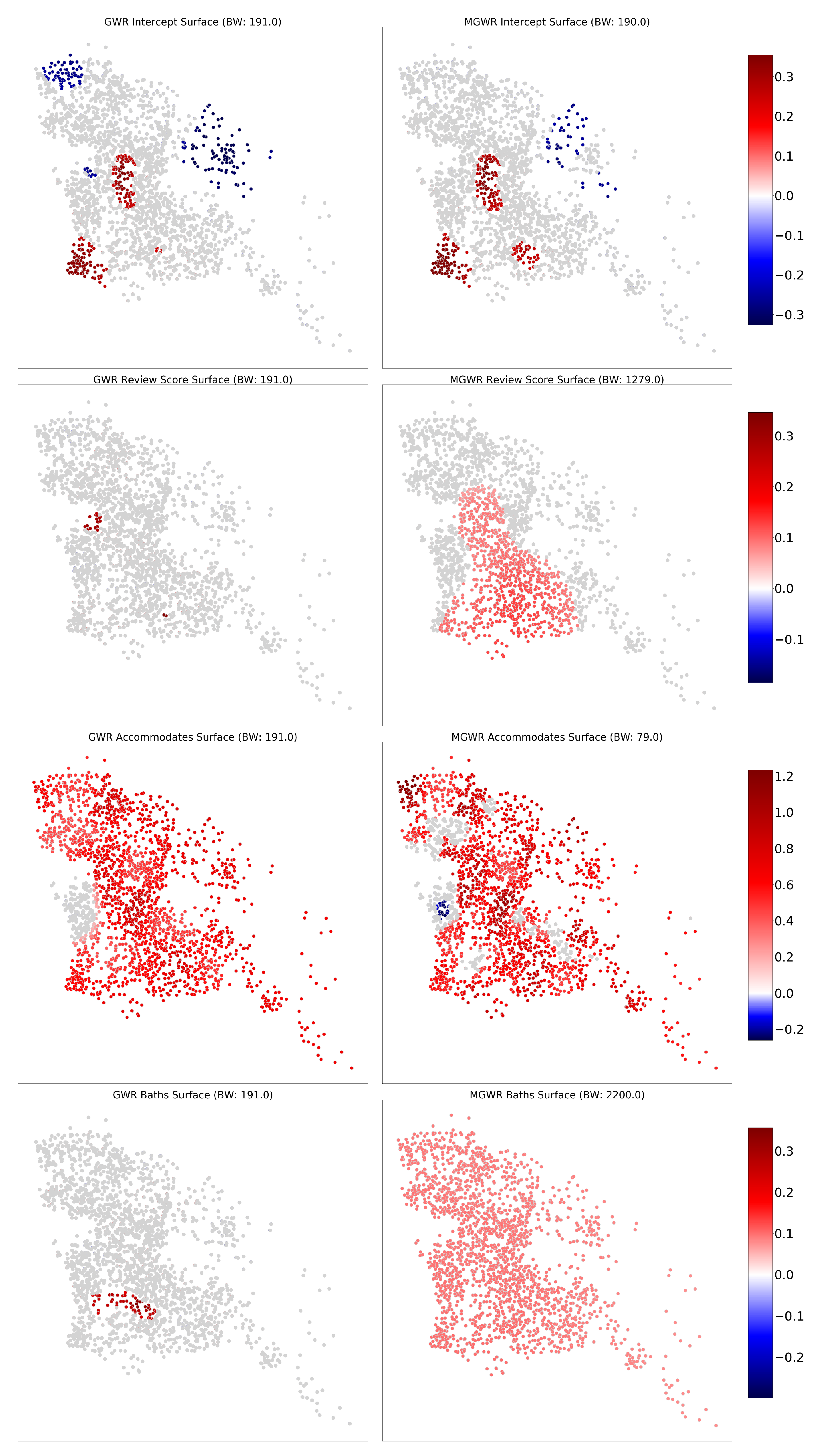
4.5.2. The Berlin Dataset

A similar analysis is available below that demonstrates inference in MGWR using the Berlin dataset and is visualized in Figure 13. As in the Georgia example above, MGWR indicates that some bandwidth estimates are similar to those from GWR: a very similar bandwidth for the intercept results in a similar pattern with two additional clusters of negative parameter estimates in the north and east; and a slightly smaller bandwidth for the accommodates variable results in fewer statistically significant parameters but with a similar pattern and the addition of a small cluster of negative parameter estimates. However, there are also some differences in MGWR bandwidths from GWR bandwidths: much larger bandwidths for the bathrooms variable and the review score variable produce many more statistically significant positive parameter estimates. In particular, the review score variable has a bandwidth implying almost all neighbors are considered, which results in all of the parameter estimates being statistically significant and remarkably constant (i.e., a global relationship) across the study area. These results reinforce that when MGWR and GWR estimate similar bandwidths, then they produces similar parameter estimates and inferences; however, when they diverge it is possible to obtain much different results. Therefore, it is necessary to utilize MGWR to ensure the correct data-borrowing scales are employed for each relationship.

#Calibrate GWR using standardized~data

>>> gwr_selector = Sel_BW(b_coords, b_y, b_X)

>>> gwr_bw = gwr_selector.search()

>>> print(gwr_bw)

191.0

>>> gwr_model = GWR(b_coords, b_y, b_X, gwr_bw)

>>> gwr_results = gwr_model.fit()

#Prepare GWR results for~mapping

#Add GWR parameters to GeoDataframe

>>> prenz[‘gwr_intercept’] = gwr_results.params[:, 0]

>>> prenz[‘gwr_score’] = gwr_results.params[:, 1]

>>> prenz[‘gwr_accom’] = gwr_results.params[:, 2]

>>> prenz[‘gwr_baths’] = gwr_results.params[:, 3]

#Obtain t-vals filtered based on multiple testing correction

>>> gwr_filtered_t = gwr_results.filter_tvals()

#Calibrate MGWR~model

>>> mgwr_selector = Sel_BW(b_coords, b_y, b_X, multi = True)

>>> mgwr_bw = mgwr_selector.search(multi_bw_min = [2])

>>> print(mgwr_bw)

[190.0, 1279.0, 79.0, 2200.0]

>>> mgwr_results = MGWR(b_coords, b_y, b_X, mgwr_selector).fit()

#Prepare MGWR results for~mapping

#Add MGWR parameters to GeoDataframe

>>> prenz[‘mgwr_intercept’] = mgwr_results.params[:, 0]

>>> prenz[‘mgwr_score’] = mgwr_results.params[:, 1]

>>> prenz[‘mgwr_accom’] = mgwr_results.params[:, 2]

>>> prenz[‘mgwr_baths’] = mgwr_results.params[:, 3]

#Obtain t-vals filtered based on multiple testing correction

>>> mgwr_filtered_t = mgwr_results.filter_tvals()

>>> kwargs1 = {‘edgecolor’: ‘lightgrey’, ‘markersize’: 175}

>>> kwargs2 = {‘facecolor’: ‘lightgrey’, ‘markersize’: 175}

>>> compare_surfaces(prenz, ‘gwr_intercept’, ‘mgwr_intercept’,

                 gwr_filtered_t[:, 0], gwr_bw,

                 mgwr_filtered_t[:, 0], mgwr_bw[0],

                 ‘Intercept’, kwargs1, kwargs2, savefig = ‘b1’)

>>> compare_surfaces(prenz, ‘gwr_score’, ‘mgwr_score’, gwr_filtered_t[:, 1],

                 gwr_bw, mgwr_filtered_t[:, 1], mgwr_bw[1],

                 ‘Review Score’, kwargs1, kwargs2, savefig = ‘b2’)

>>> compare_surfaces(prenz, ‘gwr_accom’, ‘mgwr_accom’, gwr_filtered_t[:, 2],

                 gwr_bw, mgwr_filtered_t[:, 2], mgwr_bw[2],

                 ‘Accommodates’, kwargs1, kwargs2, savefig = ‘b3’)

>>> compare_surfaces(prenz, ‘gwr_baths’, ‘mgwr_baths’, gwr_filtered_t[:, 3],

                 gwr_bw, mgwr_filtered_t[:, 3], mgwr_bw[3],

                 ‘Baths’, kwargs1, kwargs2, savefig = ‘b4’)

4.6. Local Multicollinearity

Allowing bandwidths to be distinct for each relationship can also have consequences for local multicollinearity. When each relationship is specified with the same kernel function and bandwidth parameter, it implies that they are subject to the same weighting transformation, which may exacerbate collinearity between variables and is sometimes called concurvity. By allowing bandwidths to vary, it becomes possible that variables are subject to different transformations, which can avoid inducing multicollinearity/concurvity. The local condition number is easy to extend from the GWR context to the MGWR context because it can be computed directly on the design matrix where each column is a variable and can be subjected to its respective spatially weighted transformation. The example below demonstrates the differences between local conditions numbers for GWR and MGWR for the Berlin dataset. In Figure 14 it is apparent that once the bandwidths are allowed to vary in MGWR (right) the local condition numbers are lower than for GWR (left) where the bandwidths are not allowed to vary. However, it is also apparent that for this given example, none of the local condition numbers suggest that multicollinearity is an issue since they are all below the rule of thumb of 30. Comber et al. [22] also provide evidence that the use of different distance metrics, which implies varying bandwidths, can effect the degree of local multicollinearity in (M)GWR. To the best of knowledge of the authors, the functionality presented here is the first tool available to explicitly examine local multicollinearity in the context of MGWR.

#Prepare GWR/MGWR condition number for mapping

>>> gwr_lc = gwr_results.local_collinearity()

>>> mgwr_lc = mgwr_results.local_collinearity()

>>> prenz[‘gwr_cn’] = gwr_lc[2]

>>> prenz[‘mgwr_cn’] = mgwr_lc[0]

>>> fig, axes = plt.subplots(nrows = 1, ncols = 2, figsize = (10, 5))

>>> ax0 = axes[0]

>>> ax0.set_title(‘GWR Condition Number’, fontsize = 10)

>>> ax1 = axes[1]

>>> ax1.set_title(‘MGWR Condition Number’, fontsize = 10)

>>> cmap = mpl.cm.RdYlBu

>>> vmin = np.min([prenz[’gwr_cn’].min(), prenz[‘mgwr_cn’].min()])

>>> vmax = np.max([prenz[’gwr_cn’].max(), prenz[‘mgwr_cn’].max()])

>>> if (vmin < 0) & (vmax < 0):

      cmap = truncate_colormap(cmap, 0.0, 0.5)

>>> elif (vmin > 0) & (vmax > 0):

      cmap = truncate_colormap(cmap, 0.5, 1.0)

>>> sm = plt.cm.ScalarMappable(cmap = cmap,

                      norm = plt.Normalize(vmin = vmin,

                                     vmax = vmax))

>>> prenz.plot(‘gwr_cn’, cmap = sm.cmap, ax = ax0,

           vmin = vmin, vmax = vmax,

           **{‘edgecolor’: ‘lightgrey’,

             ‘alpha’: .95,

             ‘linewidth’: .75})

>>> prenz.plot(‘mgwr_cn’, cmap = cmap, ax = ax1,

           vmin = vmin, vmax = vmax,

           **{‘edgecolor’: ‘lightgrey’,

             ‘alpha’: .95,

             ‘linewidth’: .75})

>>> fig.tight_layout()

>>> fig.subplots_adjust(right = 0.9)

>>> cax = fig.add_axes([0.92, 0.14, 0.03, 0.75])

>>> sm._A = []

>>> cbar = fig.colorbar(sm, cax = cax)

>>> cbar.ax.tick_params(labelsize = 10)

>>> ax0.get_xaxis().set_visible(False)

>>> ax0.get_yaxis().set_visible(False)

>>> ax1.get_xaxis().set_visible(False)

>>> ax1.get_yaxis().set_visible(False)

>>> plt.savefig(’compare_collin’)

>>> plt.show()

5. Additional Features

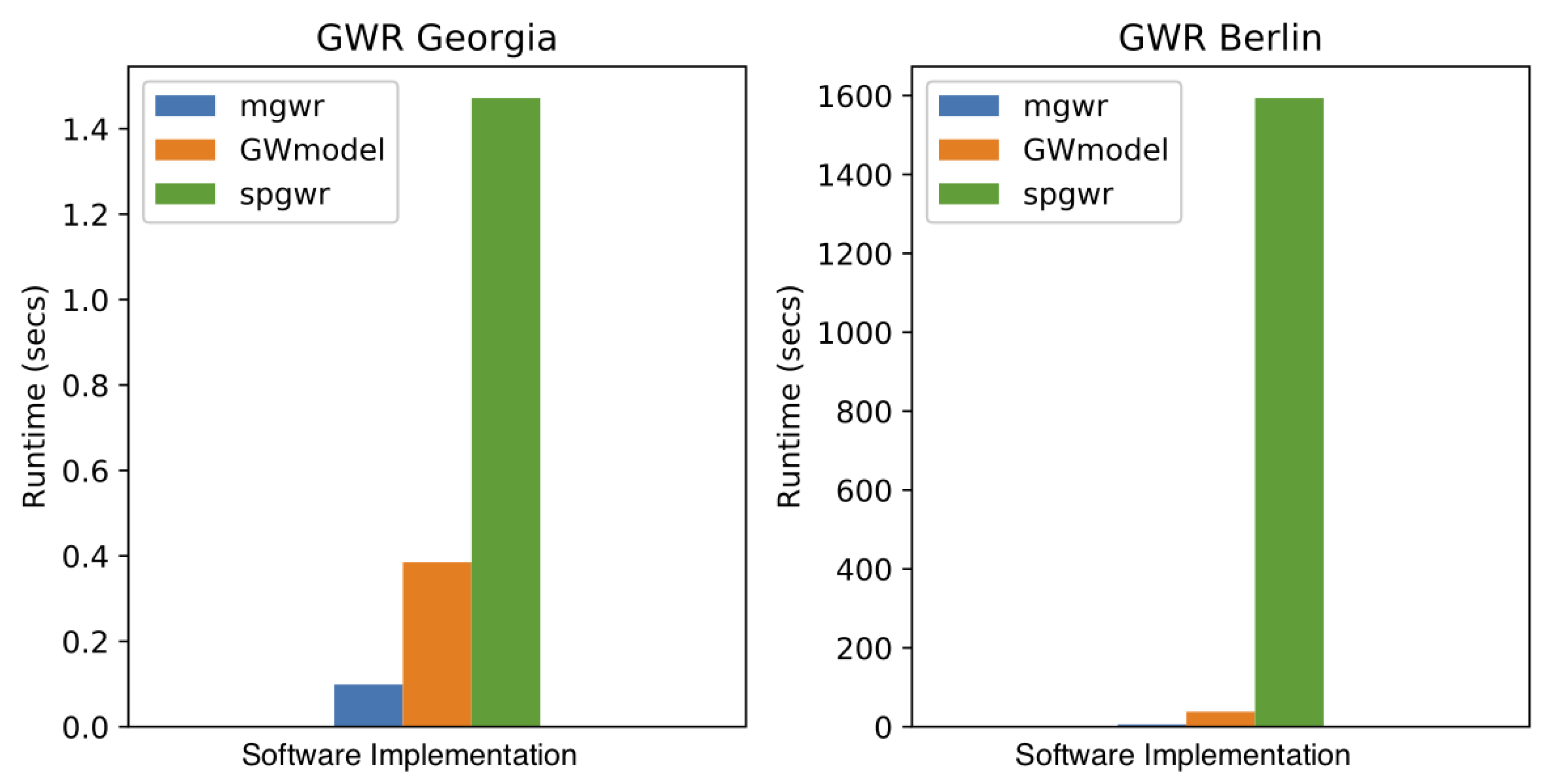
5.1. Computational Efficiency

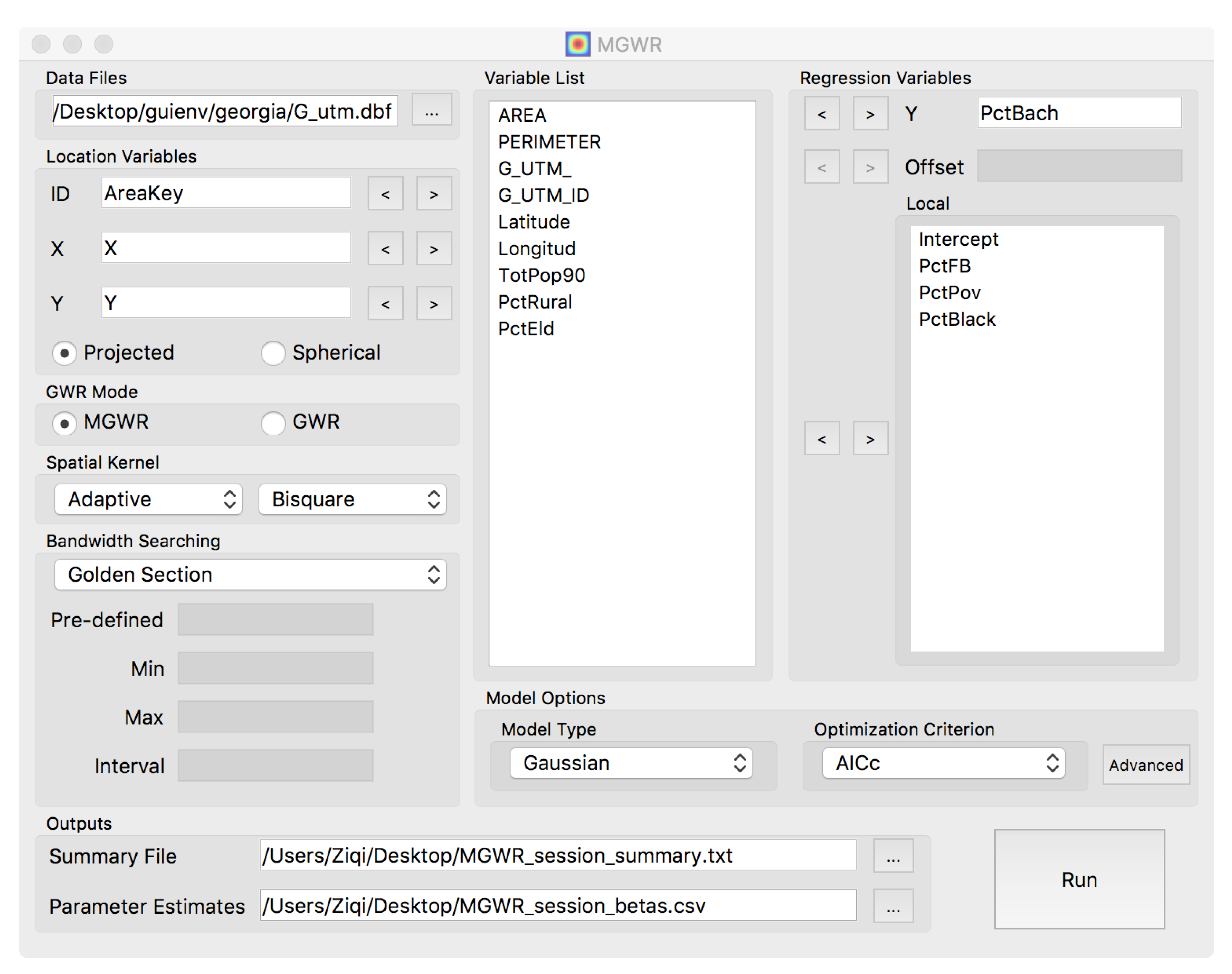
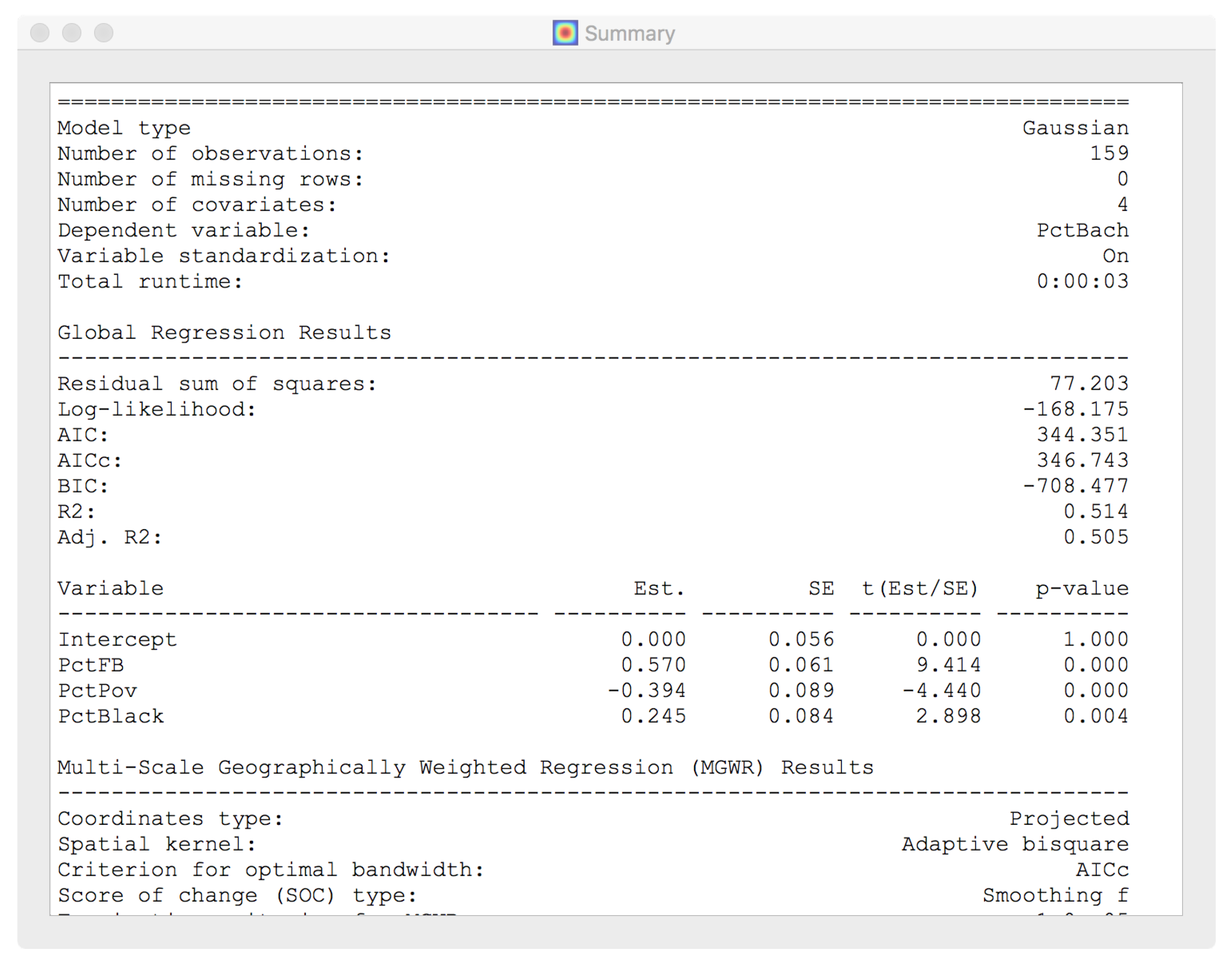
Since GWR and MGWR are based on an ensemble of local regressions, the computational overhead can become large as the number of observations and calibration locations increase. Therefore, it is important to consider computational efficiency and is often of interest to understand the advantages of different software implementations for carrying out similar tasks. Here mgwr is highlighted for its computational efficiency compared to two other actively maintained open source implementations: GWmodel and spgwr. Figure 15 compares the runtime of GWR calibrations from mgwr, GWmodel, and spgwr for both the Georgia and Berlin datasets. Each implementation was used to calibrate a model employing an adaptive bi-square spatial kernel and golden section search based on AICc minimization using the variables discussed above (i.e., 3 explanatory variables for each model). Computations were carried out on a MacBook Pro with a 2.8 GHz Intel Core i7 CPU (4 cores) and 16 GB of 1600 MHz DDR3 RAM. It can be seen that for GWR calibrated on the smaller Georgia dataset, mgwr is approximately 4× faster than GWmodel and 15× faster than spgwr and for the larger Berlin dataset, mgwr is around 6× faster than GWmodel and 262× faster than spgwr. Results show that not only is mgwr the fastest among the three for those two datasets, but it is also the most scalable. This is because mgwr incorporates algorithmic optimizations introduced by FastGWR [10], a streamlined GWR implementation that can scale to millions of observations using parallelization. Specifically, the computational overhead is lowered by minimizing the calculation of unnecessary model diagnostics during bandwidth selection search procedures.

These computational savings also extend to MGWR since the backfitting algorithm used for calibration entails a series of GWR calibrations. Figure 16 demonstrates how these optimizations result in a faster runtime for MGWR calibrations for both the Georgia and Berlin datasets in mgwr compared to GWmodel using the same model specification and computing equipment as above. Despite the fact that GWmodel does not compute MGWR parameter estimate inference diagnostics (version 2.0-6 was utilized as it was the most recent version at the time this research was carried out), mgwr is still around 1.6x faster than GWmodel for the Georgia dataset and around 3.2× faster for the Berlin dataset. No comparison is made with spgwr because it does not support MGWR calibration. It is also worth noting that GWmodel does not use the same back-fitting algorithm as proposed in [3] and instead uses an ad-hoc optimization strategy introduced in [21]. The strategy assumes that each covariate-specific bandwidth will no longer change once it is stable for two iterations of the backfitting process. However, the robustness of this optimization has not yet been demonstrated widely and is therefore not featured within mgwr.

5.2. Accessibility

A feature that is unique to mgwr is that a graphical user interface (GUI) was developed on top of the open source code base to make the functionality more accessible and is supported for both Windows and Mac operating systems. The main interface of the GUI is demonstrated in Figure 17 and allows both GWR and MGWR to be calibrated by reading in a data table (e.g., comma-separated values files, Excel spreadsheet or database file) and using point-and-click functionality to specify a desired model and calibration routine. In addition, all of the diagnostics outlined here can also be computed using the GUI. Once the routine is complete, a summary file of both global and local diagnostics is produced (Figure 18), as well as a table of the parameter estimates, their associated inference diagnostics (i.e., standard errors and t-values), predicted values, and residuals.

6. Conclusions

This paper introduced mgwr, a Python-based implementation for efficiently calibrating a variety of GWR and MGWR models and a selection of novel diagnostics that focus on capturing and interpreting multiscale spatial heterogeneity. In the presentation of these models, we suggested a few best practices for the estimation and interpretation of GWR/MGWR using the mgwr package. These include the use of “adaptive kernels” whose width adjusts to non-uniform spatially distributed samples, incorporating multiple scales of analysis using MGWR over GWR, the use of standardized variables and bisquare kernels to increase the interpretability of process scale, and the use of a proper MGWR hat matrix for rigorous model estimation and inference. The discussion of these best practices provides a useful set of suggestions for applied research.

After introducing these best practices in addition to how to enact them in the mgwr software, we demonstrated suggested usage on the Georgia and Berlin datasets. In the case of the Georgia dataset, allowing for multiple scales of analysis through the use of MGWR does not strongly affect most of the resulting parameter estimates surfaces because the estimated covariate-specific bandwidths are relatively similar to the single average bandwidth acquired through the use of GWR. In contrast, an analysis of the Berlin data set demonstrates that when the bandwidths estimated via MGWR strongly differ in magnitude from the bandwidth estimated by GWR, then the parameter estimate surfaces and the associated tests of significance may also diverge. Overall, this highlights the necessity to ensure the correct data-borrowing scales are employed for each relationship in a local model, which can be achieved through the use of MGWR.

Though mgwr provides the fastest GWR and MGWR implementations, there are still several future enhancements that could improve the package and advance the state-of-the-art in multiscale spatial analysis. First, diagnostic tests based on Monte Carlo simulations, such as the tests for spatial variability of parameter estimate surfaces could be optimized. These tests are extremely computational and can take a very long time to run for even modest sample sizes. Second, additional local multicollinearity measures could be extended to MGWR other than the local condition number. Third, out-of-sample prediction functionality could be extended to MGWR as is currently available for GWR. Fourth, probability models for discrete and binary outcomes could be adapted to the MGWR framework. Finally, MGWR calibration could be made even more scalable by incorporating FastGWR parallelization strategies [10]. These additions would make multiscale spatial analysis even more accessible and robust for use in a wider array of application domains and scopes.

References

1. Tobler, W.R. A Computer Movie Simulating Urban Growth in the Detroit Region. Econ. Geogr. 1970, 46, 234. [Google Scholar] [CrossRef]
2. Fotheringham, A.S.; Brunsdon, C.; Charlton, M. Geographically Weighted Regression: The Analysis of Spatially Varying Relationships; John Wiley & Sons: Hoboken, NJ, USA, 2002. [Google Scholar]
3. Fotheringham, A.S.; Yang, W.; Kang, W. Multi-Scale Geographically Weighted Regression. Ann. Am. Assoc. Geogr. 2017, 107, 1247–1265. [Google Scholar]
4. Environmental Systems Research Institute (ESRI). ArcMap 10.3 Spatial Analyst Toolbox; ESRI: Redlands, CA, USA, 2018. [Google Scholar]
5. Bivand, R.; Yu, D.; Nakaya, T.; Garcia-Lopez, M.A. spgwr: Geographically Weighted Regression, R package version 0.6-32; 2017. [Google Scholar]
6. Wheeler, D. gwrr: Fits Geographically Weighted Regression Models with Diagnostic Tools, R package version 0.2-1; 2013. [Google Scholar]
7. Yu, H.; Fotheringham, A.S.; Li, Z.; Oshan, T.; Kang, W.; Wolf, L.J. Inference in multiscale geographically weighted regression. Geogr. Anal. 2019. [Google Scholar] [CrossRef]
8. Lu, B.; Harris, P.; Charlton, M.; Brundson, C.; Nayaka, T.; Gollini, I. GWmodel: Geographically-Weighted Models, R package version 2.0-5; 2018. [Google Scholar]
9. Lu, B.; Brunsdon, C.; Charlton, M.; Harris, P. Geographically weighted regression with parameter-specific distance metrics. Int. J. Geogr. Inf. Sci. 2017, 31, 982–998. [Google Scholar] [CrossRef]
10. Li, Z.; Fotheringham, A.S.; Li, W.; Oshan, T. Fast Geographically Weighted Regression (FastGWR): A Scalable Algorithm to Investigate Spatial Process Heterogeneity in Millions of Observations. Int. J. Geogr. Inf. Sci. 2018. [Google Scholar] [CrossRef]
11. Griffith, D.A. Spatial-filtering-based contributions to a critique of geographically weighted regression (GWR). Environ. Plan. A 2008, 40, 2751–2769. [Google Scholar] [CrossRef]
12. Da Silva, A.R.; Fotheringham, A.S. The Multiple Testing Issue in Geographically Weighted Regression: The Multiple Testing Issue in GWR. Geogr. Anal. 2015. [Google Scholar] [CrossRef]
13. Wheeler, D.; Tiefelsdorf, M. Multicollinearity and correlation among local regression coefficients in geographically weighted regression. J. Geogr. Syst. 2005, 7, 161–187. [Google Scholar] [CrossRef]
14. Belsey, D.A.; Kuh, E.; Welsch, R.E. Regression Diagnostics: Identifying Influential Data and Sources of Collinearity; Wiley: New York, NY, USA, 1980. [Google Scholar]
15. O’brien, R.M. A Caution Regarding Rules of Thumb for Variance Inflation Factors. Qual. Quant. 2007, 41, 673–690. [Google Scholar] [CrossRef]
16. Wheeler, D.C. Diagnostic Tools and a Remedial Method for Collinearity in Geographically Weighted Regression. Environ. Plan. A 2007, 39, 2464–2481. [Google Scholar] [CrossRef]
17. Fotheringham, A.S.; Oshan, T.M. Geographically weighted regression and multicollinearity: Dispelling the myth. J. Geogr. Syst. 2016, 18, 303–329. [Google Scholar] [CrossRef]
18. Oshan, T.M.; Fotheringham, A.S. A Comparison of Spatially Varying Regression Coefficient Estimates Using Geographically Weighted and Spatial-Filter-Based Techniques: A Comparison of Spatially Varying Regression. Geogr. Anal. 2017. [Google Scholar] [CrossRef]
19. Murakami, D.; Lu, B.; Harris, P.; Brunsdon, C.; Charlton, M.; Nakaya, T.; Griffith, D.A. The importance of scale in spatially varying coefficient modeling. arXivt 2017, arXiv:1709.08764. [Google Scholar] [CrossRef]
20. Harris, P.; Fotheringham, A.S.; Crespo, R.; Charlton, M. The Use of Geographically Weighted Regression for Spatial Prediction: An Evaluation of Models Using Simulated Data Sets. Math. Geosci. 2010, 42, 657–680. [Google Scholar] [CrossRef]
21. Lu, B.; Yang, W.; Ge, Y.; Harris, P. Improvements to the calibration of a geographically weighted regression with parameter-specific distance metrics and bandwidths. Comput. Environ. Urban Syst. 2018. [Google Scholar] [CrossRef]
22. Comber, A.; Chi, K.; Quang Huy, M.; Nguyen, Q.; Lu, B.; Huu Phe, H.; Harris, P. Distance metric choice can both reduce and induce collinearity in geographically weighted regression. Environ. Plan. B Urban Anal. City Sci. 2018. [Google Scholar] [CrossRef]
Figure 1. The 159 counties within the state of Georgia. Note: basemap and scalebar added using additional code.
Ijgi 08 00269 g001
Figure 2. 2203 rental properties in the Prenzlauer Berg neighborhood of Berlin. Note: basemap and scalebar added using additional code.
Ijgi 08 00269 g002
Figure 3. Examples of exponential kernels (top), Guassian kernels (middle), and bisquare kernels (bottom) for a small, medium, and large bandwidth parameter.
Ijgi 08 00269 g003
Figure 4. Reproduced from [2]. Examples of fixed (left) and adaptive (right) bandwidth kernels.
Ijgi 08 00269 g004
Figure 5. Spatial heterogeneity of the percent rural parameter surface for the Georgia dataset using different bandwidths.
Ijgi 08 00269 g005
Figure 6. Spatial variation of local R 2 model fit statistic for the Georgia dataset. Model fit is highest in the north, and worst in the Southwest.
Ijgi 08 00269 g006
Figure 7. Parameter estimates for foreign born variable (left), composite of significant and insignificant (grey) parameter estimates without correction for multiple dependent hypothesis tests (middle) and with correction for multiple dependent hypothesis tests (right).
Ijgi 08 00269 g007
Figure 8. Surfaces of local correlation coefficients (LCC).
Ijgi 08 00269 g008
Figure 9. Surfaces of local variation inflation factors (VIF).
Ijgi 08 00269 g009
Figure 10. Surface of local condition number.
Ijgi 08 00269 g010
Figure 11. Surfaces of local variance decomposition proportions (VDP).
Ijgi 08 00269 g011
Figure 12. Parameter estimates for geographically weighted regression (GWR) (left) and multiscale GWR (MGWR) (right) for Georgia dataset.
Ijgi 08 00269 g012
Figure 13. Parameter estimates for GWR (left) and MGWR (right) for Berlin dataset.
Ijgi 08 00269 g013
Figure 14. Local condition numbers for GWR (left) and MGWR (right) for the Berlin data set.
Ijgi 08 00269 g014
Figure 15. GWR runtime comparison among mgwr, GWmodel and spgwr software implementations.
Ijgi 08 00269 g015
Figure 16. MGWR runtime comparison between mgwr and GWmodel software implementations.
Ijgi 08 00269 g016
Figure 17. Graphical user interface main window for desktop software built on top of mgwr implementation.
Ijgi 08 00269 g017
Figure 18. Summary of MGWR calibration using graphical user interface that includes global and local model diagnostics.
Ijgi 08 00269 g018