Feature Extraction and Selection of Sentinel-1 Dual-Pol Data for Global-Scale Local Climate Zone Classification


1
Signal processing in Earth observation (SiPEO), Technische Universität München (TUM), 80333 Munich, Germany
2
Remote Sensing Technology Institute (IMF), German Aerospace Center (DLR), 82234 Weßling, Germany
3
Helmholtz-Zentrum Dresden-Rossendorf (HZDR), Helmholtz Institute Freiberg for Resource Technology (HIF), Exploration, D-09599 Freiberg, Germany
*
Author to whom correspondence should be addressed.
ISPRS Int. J. Geo-Inf. 2018, 7(9), 379; https://doi.org/10.3390/ijgi7090379
Submission received: 31 July 2018
/
Revised: 7 September 2018
/
Accepted: 10 September 2018
/
Published: 18 September 2018
(This article belongs to the Special Issue Data Mining and Feature Extraction from Satellite Images and Point Cloud Data)
Abstract
:The concept of the local climate zone (LCZ) has been recently proposed as a generic land-cover/land-use classification scheme. It divides urban regions into 17 categories based on compositions of man-made structures and natural landscapes. Although it was originally designed for temperature study, the morphological structure concealed in LCZs also reflects economic status and population distribution. To this end, global LCZ classification is of great value for worldwide studies on economy and population. Conventional classification approaches are usually successful for an individual city using optical remote sensing data. This paper, however, attempts for the first time to produce global LCZ classification maps using polarimetric synthetic aperture radar (PolSAR) data. Specifically, we first produce polarimetric features, local statistical features, texture features, and morphological features and compare them, with respect to their classification performance. Here, an ensemble classifier is investigated, which is trained and tested on already separated transcontinental cities. Considering the challenging global scope this work handles, we conclude the classification accuracy is not yet satisfactory. However, Sentinel-1 dual-Pol SAR data could contribute the classification for several LCZ classes. According to our feature studies, the combination of local statistical features and morphological features yields the best classification results with 61.8% overall accuracy (OA), which is 3% higher than the OA produced by the second best features combination. The 3% is considerably large for a global scale. Based on our feature importance analysis, features related to VH polarized data contributed the most to the eventual classification result.
1. Introduction
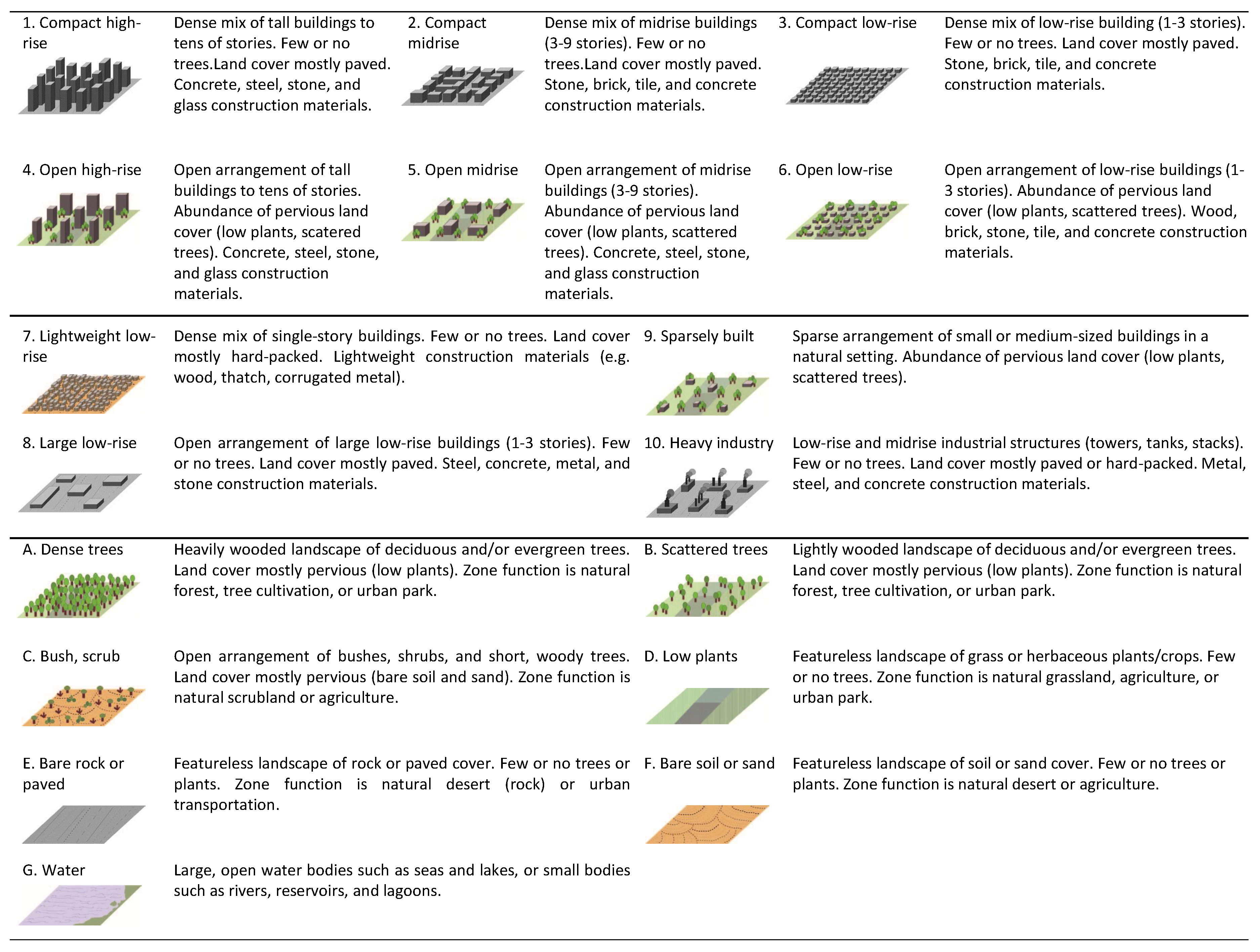
The local climate zone (LCZ) classification system is designed as a categorical scheme with 17 classes that describe urban landscapes [1,2]. These classes are defined based on surface structures and surface covers, which are specifically (1) the height of the surface structure, (2) spatial density of the surface structure, and (3) covering material of the surface (i.e., as shown in Figure 1). Eventually, the scheme yields thematic maps of a 100-m ground sampling distance (GSD), with each pixel labeled as one of the 17 classes. The LCZ was designed for the study of urban temperature behavior. It provides a research framework for urban heat island studies and standardizes the worldwide exchange of urban temperature observations [1]. As also shown in Figure 1, the scheme essentially demonstrates morphological structures of urban local neighborhood. The urban morphological structure is an influential factor on thermal behaviour. It may also reveal the economic status and the population distribution of a particular city. For example, slum districts, which are less economically developed regions with massive population concentration, normally appear as the seventh class in Figure 1. Therefore, thanks to the described morphological structure, the LCZ map acts as a valuable source for a wide variety of studies in urban areas.
Following the introduction of LCZs, the World Urban Database and Portal (WUDAPT, http://www.wudapt.org) was initiated [3,4]. WUDAPT has been mainly developed by researchers to obtain high-quality land-cover/land-use information globally, usually via crowdsourcing [5,6], games [7], or other challenges [8]. The WUDAPT project presents a suggested workflow to produce the LCZ map by taking advantage of remote sensing techniques. The production process briefly functions as follows [3]: First, the region of interest (ROI) for a particular city is defined and labels of all classes are manually selected. Second, multispectral images captured by LandSat-8 are prepared for the ROI of the target city. Finally, a supervised classification (i.e., random forest [9]) is applied to the multispectral data to produce the final classification map. Besides the standard production of the WUDAPT project, studies of LCZ classification mainly focus on using optical remote sensing data [10,11,12].
One of the key factors to define LCZ classes is height. A few studies on LCZ classification were introduced to fuse the digital surface model (DSM) with the optical data in order to use both height and spectral information [13,14]. The Thematic Mapper (TM) data captured by LandSat-5 and Enhanced Thematic Mapper Plus (ETM+) data of LandSat-7 were fused with the normalized digital surface model (NDSM) and airborne Interferometric Synthetic Aperture Radar (InSAR) using feature concatenation and then applied to multiple classifiers for LCZ-related classification in [13]. In [14], LandSat-8 data and the digital surface model (DSM) were also concatenated at the feature level and then classified by a random forest and support vector machine [15]. It was concluded that spectral features can significantly contribute to the classification task. Geographical information system (GIS)-based approach is also developed to produce the LCZ map in [16,17,18]. Although Open Street Map (OSM) provides a free-accessible GIS dataset, the completeness of the GIS data needs to be improved, especially for the developing countries. Besides the aforementioned data sources, the Sentinel-1 mission provides a dual-polarimetric synthetic aperture radar (dual-Pol SAR) with free access and global coverage. It has also been studied for LCZ classification in [19]. Researchers have proven that the combination of Sentinel-1 dual-Pol data and LandSat-8 data can improve the performance of LCZ classification. However, they only take used of amplitudes of VV and VH channels and their corresponding texture features derived by gray-level co-occurrence matrix (GLCM). Amplitudes of the two channels only constitute one part of the polarimetric information provided by the dual-Pol data. One important feature, the coherence of the two channels, is missing. Therefore, the first goal of this work is to comprehensively investigate the polarimetric information of Sentinel-1 dual-Pol data for the LCZ classification task.
Global LCZ mapping offers substantial help in exploring local climates on regional and worldwide scales. Several studies have successfully produced LCZ classification maps corresponding to one city by only labeling samples of that city. In this manner, the produced classification maps have achieved high classification accuracy (e.g., overall accuracies (OAs) are beyond 80%) since both training and test samples are located in the same city. However, the collection of accurate training samples are either expensive or time-demanding. Therefore, in the remote sensing community, there is great interest in training models based on the samples available for some cities and applying the trained models to other cities. However, this is a challenging task. For example, one study [20] attempted to select training samples from one city for the classification of another city using RF. The classification accuracies dropped to 18.2%, which indicates that the knowledge transferability between different cities should be carefully considered. In this regard, our second goal is to develop a classifier with adequate generalization capability to be applied to any other cities. The difficulty in this task lies in that the classifier needs to be trained using a limited number of training samples while remaining applicable to handling transcultural, transnational, and cross-environmental data in a worldwide context.
To cope with the aforementioned challenge of generalization, the 2017 Geoscience and Remote Sensing Society (GRSS) data fusion contest of the year 2017 proposed training the classifier on five cities (Berlin, Hong Kong, Paris, Rome, and Sao Paulo) and testing the results on four other cities (Amsterdam, Chicago, Madrid, and Xi’an). Although deep learning-based classification methods have proven to be strong in terms of classification accuracy a generalization capability in the remote sensing community [21,22,23,24], the ensemble-based canonical correlation forest (CCF) classification strategy achieved the best performance in the contest, among more than 800 submissions [8,25]. Therefore, this work uses the CCF classifier to pursue a solution for our task. The CCF classifier is an advanced version of a random forest, which is a shallow classifier.
In contrast with the automatic feature selection and extraction of deep learning methods, the feature design is of key importance to shallow classifiers. From the perspective of feature space, especially for dual-Pol SAR data, a limited number of features is not adequate for a complicated classification like the LCZ task. An informative and appropriate number of features should be derived for the subsequent classification task. References [13,25] indicates that local statistical features are informative features regarding LCZ classifications. Texture features derived from GLCM have been proven to be informative for applications of SAR data [26,27,28,29,30]. Mathematical morphological features obtained from a morphological profile have been highly effective in multi/hyperspectral image classification [31,32,33]. Consequently, besides polarimetric features, we investigate the performances of local statistical features, GLCM features, and morphological profiles for LCZ classification on a global scale.
To sum up, the aims of the study are threefold for local climate zone classification. (1) Comprehensive polarimetric information of the Sentinel-1 dual-Pol data is investigated, which includes intensities of VV and VH channels as well as the coherence and relative phase of the two channels. (2) Classification on a global scale is studied by training and testing the CCF on the separated data of transcontinental cities, which involves terabytes of data volume. (3) Four features (polarimetric feature, local statistical feature, texture feature, and mathematical morphological feature) that were proven to be successful in related tasks are evaluated in our scenario of global-scale LCZ classification.
The rest of the paper is organized as follows. Section 2 demonstrates the principle of selecting a study area and describes the Sentinel-1 dual-Pol data and its data preparation. Section 3 introduces our methodology of global-scale LCZ classification. Section 4 discusses the experiment results regarding feature extraction and selection. Lastly, Section 5 concludes this work.
2. Study Area and Data Set
2.1. Study Areas
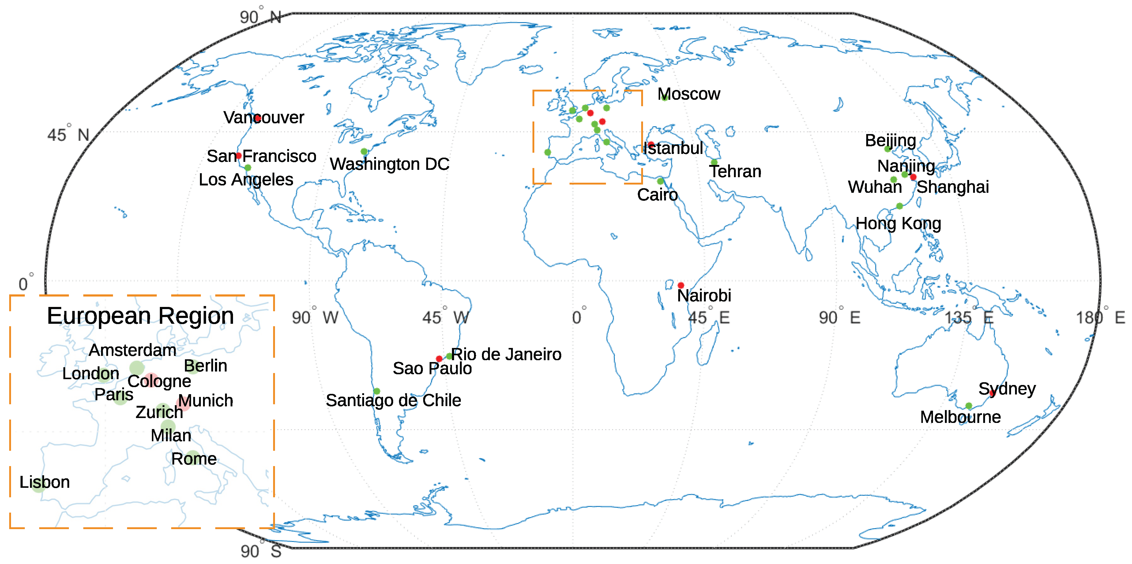
Our study aims to produce LCZ maps on a global scale and also focuses on cities of high population density. In total, 29 cities were selected and listed in Table 1. They are located on all continents except Antarctica, shown in Figure 2. This geographical distribution ensures that cities of interest include transcultural, transnational, and cross-environmental regions. While selecting these cities, population was another criteria under consideration. Among all cities, the population of each city was at least one million in 2016 and is expected to grow in the future according to UN statistics [34]. To enable our framework to solve the global challenge, cities of different regions were selected for both training and testing. The selection is shown in Figure 2 and Table 1.
2.2. Ground Truth
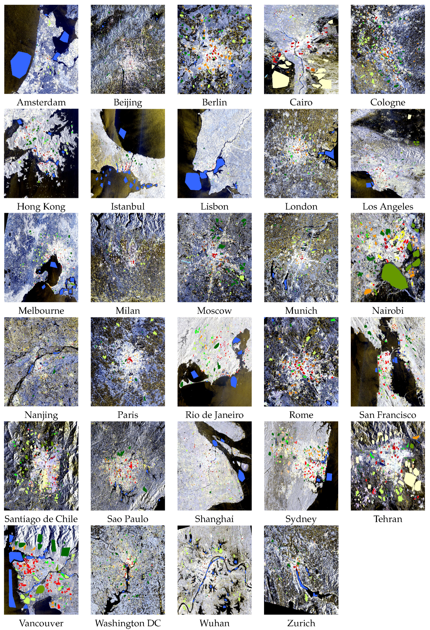
To produce LCZ classification maps in a supervised manner, we manually created the ground truth for the selected 29 cities. Generally, the labeling procedure followed the WUDAPT project standard procedure [4]. First, the region of interest (ROI) was decided for each selected city as a 50-by-50-kilometers rectangle centered at the city center. Within the rectangle, the ground truth, polygons of LCZ classes, were manually delineated by observing satellite images on Google Earth (https://www.google.com/earth/). Then, LandSat-8 images were prepared for the ROIs of each city. Afterwards, the software SAGA GIS (www.saga-gis.org/en/index.html), taking the delineated ground truth and LandSat-8 data as inputs, produced an LCZ classification map using the random forest classifier. The produced classification map is aim to be used as an additional validation source for checking the correctness and completeness of the ground truth data. By manually cross checking the classification map, images on Google Earth, and the delineated ground truth, the ground truth is modified if necessary, in the regard of correctness and completeness. Eventually, the delineated polygons of LCZ classes are created as the ground truth data, which are used for training and testing in this work. The delineated ground truth data are shown in Figure 3 with Sentinel-1 data as background.
2.3. Sentinel-1 Dual-Pol Data
The Sentinel-1 mission, as the SAR component of the European Copernicus program, has a constellation of two satellites each mounted with a C-band Synthetic Aperture Radar sensor. It has global coverage with a temporal resolution of six days. Additionally, the data is freely accessible.
The sensor collects data in four modes: (1) Stripmap (SM), (2) Interferometric Wide swath (IW), (3) Extra Wide swath (EW), and (4) Wave (WV). We used a level-1 product, which is focused single look complex data collected from the Interferometric Wide swath mode, because of its large coverage and availability. The level-1 Interferometric Wide swath SLC product consists of one image per sub-swath (three-sub-swaths, IW1, IW2, and IW3), per polarization channel (two polarization channels: VH and VV), resulting in six images in total. The properties of different swaths are shown in Table 2 while Table 3 shows the common properties of all sub-swaths.
2.4. Data Preparation
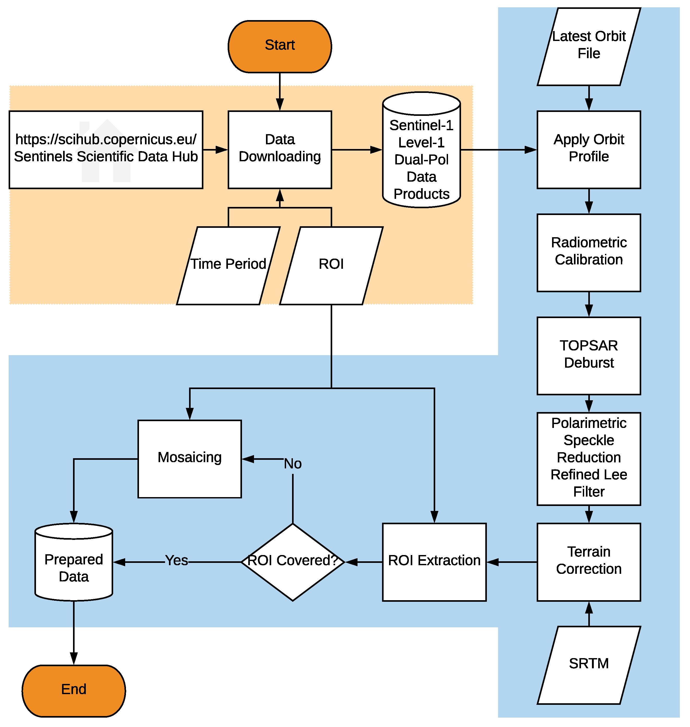
Figure 4 presents the flowchart of data preparation for this work. It generally consists of two main parts—data downloading and data preprocessing—which are indicated as orange and blue blocks, respectively.
Regarding data downloading, the Sentinel-1 data set is accessible to any users via the Copernicus Open Access Hub (https://scihub.copernicus.eu/) (also known as the Sentinels Scientific Data Hub). An open-source toolbox, named SentinelSat (https://github.com/sentinelsat/sentinelsat), provides the utilities of searching, downloading, and retrieving the metadata of Sentinel satellite images. An automatic data downloading tool was developed using SentinelSat, which functions based on an ROI file and a given time period of data collection.
For data processing, an ESA toolbox, the Sentinel Application Platform (SNAP, https://step.esa.int/main/toolboxes/snap/), was designed to work with data provided by Sentinel missions. The Sentinel-1 tool box [35] was integrated as a module to deal with all Sentinel-1 data products. The toolbox provides a powerful kit, named the graph processing tool (GPT), which is able to handle large data processing. Based on the GPT, an automatic Sentinel-1 data preprocessing chain was developed in our work so that data could be prepared for the classification task.
As shown in the flowchart, a series of data preprocessing modules are applied to Level-1 Sentinel-1 dual-Pol data products by GPT. The functionalities and configurations of these modules are explained in detail as follows:
- Apply Orbit Profile: This module of preprocessing downloads the latest released orbit profile so that a precisely geocoded product can be achieved.
- Radiometric Calibration: Radiometric calibration aims to convert the digital number of the pixel to a radiometrically calibrated backscatter, which is directly related to the radar backscatter of the scene. To extract the relative phase and the correlation between VV and VH, the product of calibration was chosen as a complex valued image.
- TOPSAR Deburst: For each polarization channel, the Sentinel-1 IW product has three swaths. Each swath image consists of a series of bursts. TOPSAR Deburst merges all these bursts and swaths into a single SLC image.
- Terrain Correction: Terrain correction eliminates the distortion introduced by the topographical variations. To accomplish the correction, the SRTM was used as the DEM to provide height information. The data was re-sampled to a 10-m GSD by the nearest-neighbor interpolation. The data was geocoded into the WGS84/UTM coordinate system, in which the manually labeled ground truth data was coordinated, so that the ground truth data and Sentinel-1 data could be matched in terms of geo-location.
After the data preprocessing, the analysis-ready dual-Pol data is organized in the common PolSAR covariance matrix. The processed Sentinel-1 dual-Pol data of 29 cities are shown in Figure 3.
3. Methodology
The main building blocks of the proposed global-scale classification approach are feature extraction and classification, which will be detailed in the following subsections.
3.1. Feature Extraction
Following the data preparation described in Section 2, the Sentinel-1 dual-Pol data was processed to the commonly used PolSAR covariance matrix, with a size of two by two. Based on the above mentioned preprocessed dual-Pol data, four different types of features were derived. They were, namely, polarimetric, local statistical, texture, and mathematical morphological feature, which will be described in the following subsections:
3.1.1. Polarimetric
SAR polarimetry allows for the retrieve of shape, orientation, and dielectric property information of scatterers [38,39]. Since there are multiple polarimetric channels, it provides more information than single-pol SAR data. However, the richness of polarimetry is achieved by sacrificing the spatial resolution. To balance the trade-off, instead of a fully polarized SAR, Sentinel-1 mission provides partially polarized SAR data, known as dual-Pol data, with the VV and VH channels. To use the polarimetric information of Sentinel-1 data, we used the intensity of the VH channel , intensity of VV channel , normalized coherence of VH and VV , and relative phase of VH and VV , where and are the complex signals of VV and VH channels, and denotes complex conjugate. These four features contain essential polarimetric information provided by the dual-Pol data. This polarimetry combination is able to distinguish specular scattering from diffuse scattering [40]. For the purpose of LCZ classification, these features are highly beneficial to differ classes with different surface roughnesses, such as water, plant, building, and soil. We named them as Pol-Baseline in our experiments.
3.1.2. Local Statistical
Since the morphological structure of an urban neighborhood is one of the essential factors that local climate zone classes try to describe, it is natural to derive features describing the local neighborhood. It has been shown that simple statistical parameters of a local neighborhood the mean and standard deviation are suitable features for the classification in [13,25]. In our global-scale task, we extracted five statistical parameters: maximum, minimum, mean, standard deviation, and median of local patches. Since the ground sampling distance (GSD) of the LCZ map was suggested to be 100 ms [3,25], the local patch in this work was defined as a size of 10 by 10 pixels, corresponding to the suggested 100 meters GSD. Those parameters were derived from all four polarimetric features (Pol-Baseline), resulting in 20 features. We named the local statistical feature the Stat-Feature.
3.1.3. Texture
In general, SAR data is well known for containing texture information [27,29,41]. Dual-Pol SAR data is even richer in this regard, simply because it has one more channel. The GLCM is used here to extract texture features. The GLCM describes the distribution of co-occurring values of an image in a given area. It provides a statistical view of texture based on the image histogram [42]. This work extracts the GLCM-based texture information from Sentinel-1 dual-Pol data for LCZ classification. The GLCM statistical features used for describing the distributions include contrast, dissimilarity, homogeneity, angular second moment, maximum probability, entropy, mean, variance, and correlation. For more details of those features, please refer to [42]. Those features can characterize specific characteristics of images, such as homogeneity, contrast, and organized structures presented in an image. For the purpose of LCZ classification, the compactness relates to the spatial distribution of deterministic scatterers in a SAR image, which can be represented by GLCM features. Thus, the GLCM-based texture features are expected to be beneficial to classify LCZ classes with respect to compactness. To compute the GLCM, it was applied to intensity images of VV and VH channels. For the computational efficiency, the intensity value was quantized into 32 bins. The orientations 0, 45, 90 and 135 were chosen. A window size of 11 pixels was chosen. Since the ground sampling distance of the data was 10 ms, the window size suits the 100-m resolution definition of the local climate zone product. The ESA SNAP toolbox was used for GLCM extraction because of its fast implementation. The feature was named the GLCM-Feature.
3.1.4. Mathematical Morphological
Spatial-contextual information also plays an important role in LCZ classification. Morphological profiles are regarded as one of the most effective techniques for the extraction of spatial-contextual features and have been intensively used in the remote sensing community for information extraction and scene classification using optical data [33,43,44,45] and SAR data [27]. Very recently, the advantage of using morphological profiles has become apparent in the application of LCZ classification [8].
The main building blocks of morphological profiles are opening and closing operation [46]. These morphological operators simplify the input gray scale image by removing structures with respect to a predefined structuring element. Structuring elements have a unique structure with a known shape and size (e.g., a disk with a radius of 5 pixels). Therefore, morphological profiles can be produced using a sequence of opening and closing operations, where a structuring element of increasing size applied to a gray scale image to accurately extract spatial features [44]. In [47], an advanced version of opening and closing (opening and closing by reconstruction) was introduced to further improve the ability of the conventional opening and closing operators in terms of information extraction and shape preservation. Opening and closing by reconstructions satisfy the following criterion: If the structuring element cannot fit the structure of the image (objects), then it will be totally removed, otherwise, it will be totally preserved. Reconstruction operators remove objects smaller than structuring element without altering the shape of those objects and reconstruct connected components from the preserved objects. Figure 5 shows an image captured over the city of Zurich along with its corresponding opening, opening by reconstruction, closing and closing by reconstruction.
The structuring element has two important parameters: shape and size. Different objects with various surroundings have different degrees of response when considering morphological profiles under different structuring element sizes and shapes. Therefore, morphological profiles can extract the spatial features under different scales and geometric properties. In this paper, the profile was produced by considering the intensity images of VV and VH as inputs. The investigated structuring element in this paper is circular with the diameters set to 1, 3, and 5. We named the morphological feature the "MP-Feature".
3.2. Classifiers
A CCF [48] was chosen to pursue a solution to the task of global local climate zone classification in this work. There are two reasons for this selection: (1) CCF, as a member of random forest methods, is a non-parametric algorithm with a low computation cost, which also provides the function of feature importance analysis; (2) CCF was proven to not only outperform other classifiers in computer vision [48] but also as highly effective in local climate zone classification [25].
To recall a CCF, necessary notations are introduced as follows. Let denote the training data, with N instances and P features. Let be the label of training data, where C is the number of classes. If , a -sized vector, indicates that data instance belongs to class two, the second element of vector equals one, and other elements are zero. Accordingly, the training data set is represented as . Similarly, let denote the data for the prediction and denote the predicted label. Differing from the label in the training data, all elements in predicted label, vector , ranges in , represent the probabilities of every class that falls under.
3.2.1. Canonical Correlation Analysis (CCA)
Canonical correlation analysis was designed to analyze the linear relation between sets of variables [49]. Let two data sets be represented as and , with k instances and the numbers of features as a and b, respectively. CCA pursues canonical coefficients and so that data sets W and V are linearly mapped into a latent space ( and ) where they have maximum correlation. Canonical coefficients are coupled in a pair-wise fashion and given by (1).
3.2.2. CCFs
As a CCF is an advanced version of random forests, it is introduced by first presenting the random forest and then explaining the improvements made by CCF.
Let denote random forests, where a random forest consists of L decision trees . An individual decision tree recursively divides a feature space by axis-aligned split until the pure node or stop criteria is achieved. Since a decision tree is a deterministic classifier, training on the same data results in identical trees. To introduce randomness, there are two general strategies among random forest methods. The first one is bagging, where subsets of the whole training data are randomly sampled with replacements for training decision trees [51]. The second strategy is to use random subspaces of original data to train decision trees [52]. Both strategies decorrelate decision trees and create diversity in predictions. Statistically, diversity encourages a random forest to follow the Law of Large Numbers so that it does not suffer from overfitting as individual decision tree [48,53,54]. Most importantly, the diversity is essential to the power of random forest. At the final prediction phase, an averaging of outputs of all trees is applied for the regression task (2).
For the classification task, besides the majority voting of a unique label, a random forest can also provide probabilities of each class that data instance falls under (3).
Regarding the CCF, there are two key improvements [48]. First, instead of splitting the feature space in axis-aligned manner, it finds the hyperplane in the projected space, where input features and training label have maximum correlation. This enables CCF to find natural class boundaries in the feature space instead of restricting it to the axis. The second improvement is called projection bootstrapping. Instead of bagging the training data, it takes in all training data. However, it selects training samples exactly as bagging does to find the CCA projections. Then, all training data are mapped into the canonical correlation space to find hyperplanes. In this fashion, diversity is introduced by bagging-learned CCA projections.
3.2.3. Feature Importance Analysis
To better understand how different features work for our global-scale LCZ classification task, the function of feature importance analysis in a CCF is applied to gain a quantitative insight. Before the analysis, the principle of feature analysis is recalled in this section.
Once a CCF is trained, it predicts the out-of-bag sample or the validation sample. With the ground truth label, one could estimate a prediction error . To achieve the importance analysis of feature , only values of feature are randomly permuted in samples. Therefore, the trained CCF predicts the label of samples with permuted and achieves another prediction error . Hypothetically, should be smaller than . The feature importance indication of is given by , where the higher the value of this indication, the more important is feature is [53].
4. Experiments and Discussion
In this section, the performance of different feature types were analyzed. In this context, firstly, the polarimetric feature and local statistical feature were quantitatively compared, and the one with better performance was later treated as a benchmark feature. Secondly, the chosen benchmark feature was combined with the texture feature and morphological feature, respectively, allowing the performance of the latter two types of features to be compared and analyzed. Afterward the feature importance was analyzed using the CCF. Lastly, the performance of the Sentinel-1 dual-Pol data was discussed regarding the application of local climate zone classification. For all following experiments, the training was based on 20 cities and the testing was conducted on 9 cities, as listed in Table 1. The performance of the classification approach is evaluated based on three quantitative indicators, overall accuracy (OA), kappa coefficient, and average accuracy (AA). OA is simply achieved by dividing the total number of correctly classified samples by the number of overall classified samples, and reported in percentage. Kappa coefficient is a statistical measurement, which estimates inter-rater agreement and is of no unit. AA is the average of all class-specific accuracies.
4.1. Benchmark Feature Selection
The Pol-Feature is the identical preprocessed dual-Pol data organized at the pixel level with a ground sampling distance of 10 by 10 ms. The Stat-Feature derives straightforward statistical parameters out of a neighborhood of 100 by 100 ms. The extent is identical to the resolution of the targeted local climate zone classification map. Although the Stat-Feature involves spatial information, it essentially describes the polarimetric feature as well. Therefore, our first experiment was to analyze performances of both features. The better one, in terms of OA and kappa, was selected as the benchmark feature, which is later combined with the GLCM-Feature and the MP-Feature for further analysis.
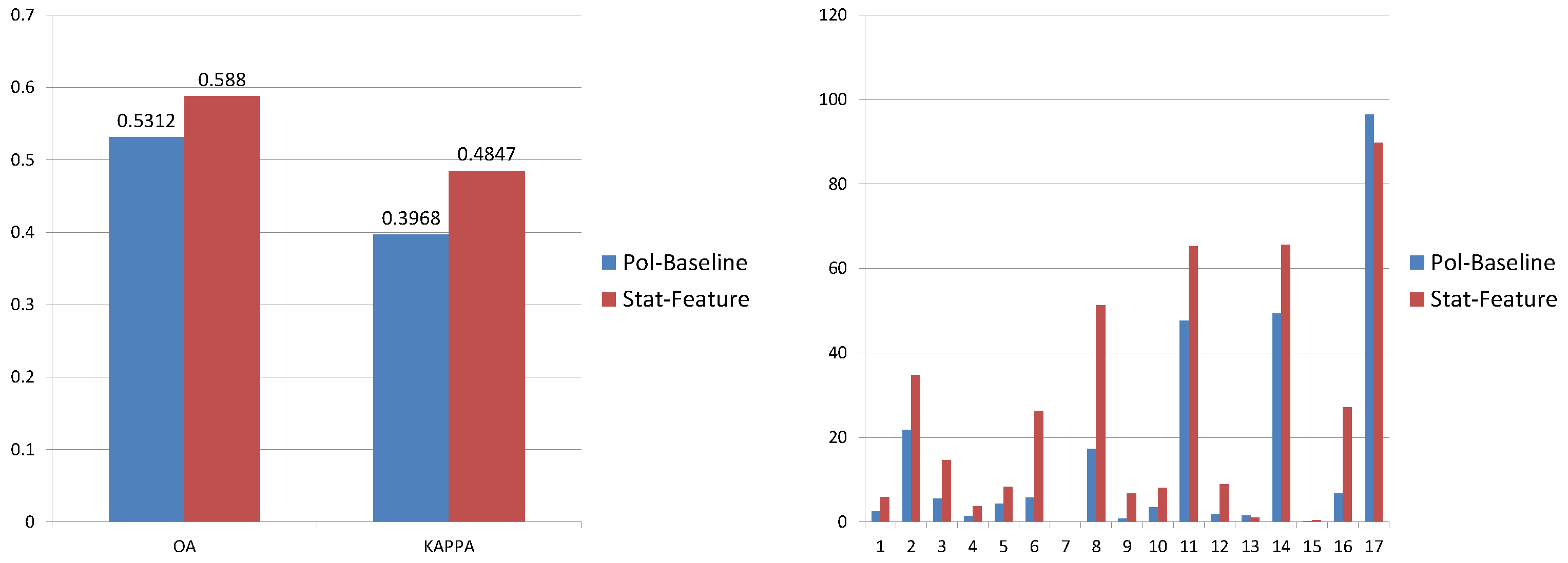
According to Figure 6, the Stat-Feature outperformed the Pol-Feature by 5.68% and 0.088, in terms of OA and the kappa coefficient, respectively. It also performed better generally on producer accuracies. Considering the challenge of global scale in our work, the difference is quite dramatic, but not surprising. It has been proven in remote sensing that involving spatial information can significantly improve the classification performance [55,56,57]. Consequently, the Stat-Feature was selected as the benchmark feature to work with the other two features.
4.2. Texture Feature
The speckle is omnipresent in SAR images as an intrinsic characteristic [58], which is normally regarded as noise during SAR data interpretation. However, when extracting texture information, the speckle becomes a valuable source containing rich texture information. To quantitatively test to what extent speckle filtering impacts texture, the GLCM-Feature was extracted from data sets with (GLCM-Feature-F) and without (GLCM-Feature-UF) speckle filtering.
To summarize results in Figure 7, firstly, by comparing classification performances of GLCM-Feature-F and GLCM-Feature-UF, speckle filtering led to a massive loss of texture information. Secondly, the GLCM-Feature downgraded the classification performance of the Stat-Feature. The reason could be as follows. (1) Originating from the GLCM design, the radiometric resolution is decreased to 32 statistically equalized bins for computational efficiency, thus causing information loss. (2) The equalized bin is statistically decided in the individual data set. For a global scale task, data sets collected from different locations, at different times, with different incident angles would have very diverse intensity responses in imageries. Therefore, the method of GLCM texture extraction is unable to ensure that data sets with the same textures appear the same in the feature space.
4.3. Morphological Feature
To set up comprehensive experiments, like GLCM-Feature extraction, the MP-Feature was applied to data sets with MP-Feature-F and without MP-Feature-UF speckle filtering. Therefore, the performance of the MP-Feature could be tested regarding speckle SAR data.
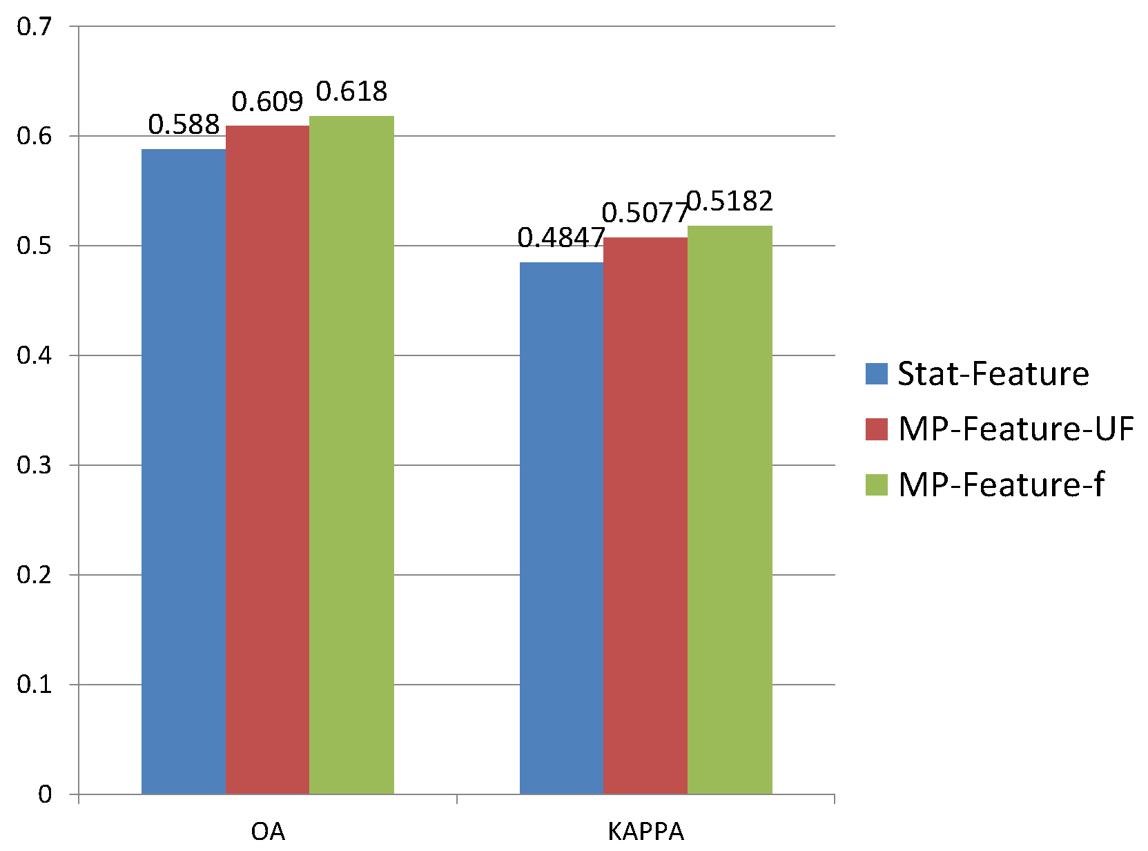
According to results shown in Figure 8, MP-Feature improved the classification by 3% in OA. Furthermore there was almost no difference in the performance between MP-Feature-UF and MP-Feature-F.
4.4. Analysis of Feature Importance
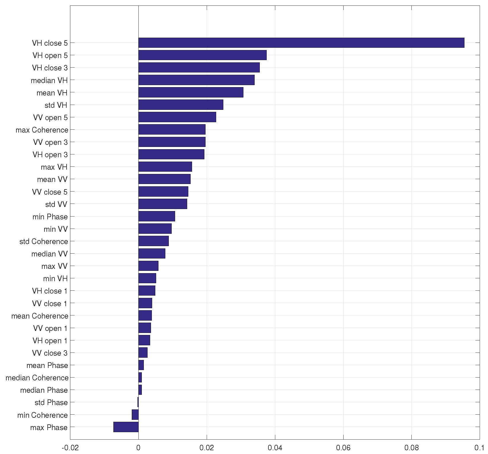
Figure 9 shows the feature importance achieved by canonical correlation forests using all test samples. The empirical importance indication reveals several interesting phenomenons. Firstly, the most important three features are components of the MP-Feature. The morphological spatial feature plays a very important role in our global LCZ classification task since LCZ classes describe the morphological property of an urban local neighborhood. Secondly, the VH polarized data contributes the most to the classification because eight out of top ten important features (all top six), are related to VH data. Thirdly, the coherence of VH and VV data also contribute the classification; however, it has often been ignored when using PolSAR data. Lastly, features on the relative phase between VV and VH barely provide any information because they are all among the least important features.
4.5. Class-Wise Analysis
Table 4 shows class-specific accuracies of different feature combinations. Table 5 gives detailed information about the combinations. In the comparison of feature combinations, class-specific accuracies, OA, and kappa suggest that classification using the Stat-Feature and MP-Feature derived from filtered data provided the best classification accuracy. By comparing feature combinations A and B, the Stat-Feature improved classification accuracies significantly. Morphological description was also very important for our classification task because adding the MP-Feature to the Stat-Feature further improved classification accuracies, by comparing combinations B and E.
Since the task is very challenging in aspects of global scale and complicated LCZ classes, with the CCF strategy, Sentinel-1 dual-Pol data were not able to provide satisfactory classification accuracies.
However, there was valuable information on how Sentinel-1 dual-Pol data could contribute to this task. Despite GLCM is not suitable on extracting textures from multiple cities, the texture features of Sentinel-1 dual-Pol data did excel in distinguishing compactness and height, because the combination C provided better accuracies for the first six classes compared to other combinations. By comparing the accuracies of bare soil or sand in combinations B and C, one can determine that a SAR speckle texture is a good option for classifying this specific class.
4.6. Sentinel-1 Data for LCZ Classification
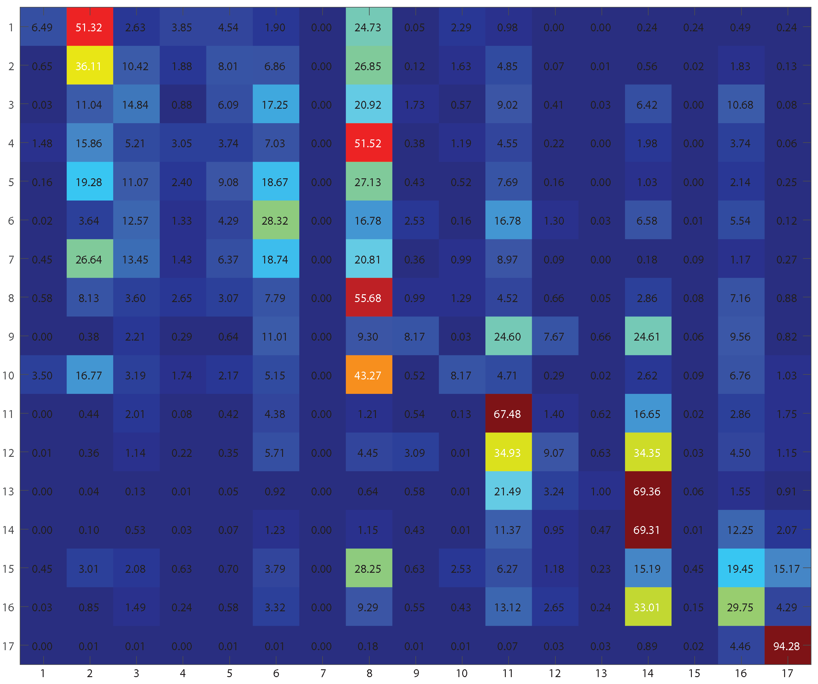
According to Table 4 and Figure 10, it is obvious that the classification accuracy is not satisfactory. With reference to the proposed working flow shown in Figure 10, the first ten urban classes are very hard to be classified with the individual use of Sentinel-1 dual-Pol data. The two classes, compact high-rise and the compact mid-rise, are confused with each other. In addition, most urban classes are confused into the class of large low-rise. Eventually only accuracies for the water, low plants, and dense trees are acceptable. However, as it is the first study of LCZ classification using Sentinel-1 dual-Pol data, the present outcome leaves rooms for improvement.
5. Conclusions
This paper describes the first attempt to produce local climate zone classification maps on a global scale using freely accessible Sentinel-1 dual-Pol data sets. The set of features, which were reported as being informative in the literature were assessed for our specific goal. We discovered that the local statistical feature excelled in optical classification and also well with dual-Pol SAR data. However, the GLCM feature, which has often been reported as highly informative in SAR classification, was not suitable for our global scale task due to the lack of a generalization capability since its dependency on a statistical distribution of an individual data set limits its transferability to other data sets. The morphological profile functioned quite well in our task, improving local statistical features, texture features by 3% and 9.29% in terms of OA. Morphological profiles extracted the spatial morphological structure of the data, which suited the essential content of local climate zone classes. According to the feature importance analysis of the CCF classifier, the VH polarized data had the biggest contribution to our classification task. The often-ignored feature, the coherence of VV and VH, contributed more to the classification compared to contributions of the VV polarised data. Moreover, the relative phase of VV and VH polarized data barely provided informative content for classifications, even dragging down the performance.
By far, classification accuracies of the Sentinel-1 data are not very appealing. However, considering the challenges of a global scale and transferability in our task, Sentinel-1 data still contributes in different manners for certain classes. The ensemble CCF strategy in this paper was chosen for the classification step due to its high generalization ability and superior performance over deep learning-based classifiers [8]. One potential reason for why CCF outperformed a deep learning-based classification method in [8] may have been due to the limited number of training samples. However, one deficiency of the CCF is that it demands hand-designed extracted features to further boost its classification performance. While endless combinations of features that can be fed to a CCF exist, this paper took the very first steps to evaluate the most informative sets of features and critically compare their performance for a global LCZ classification.
In the future, we intend to further examine this challenging task by investigating a deep learning strategy in order to take advantage of its capability of automatic feature extraction and selection. No matter which strategy is under consideration, one more critical detail should also be studied is that, how large is the neighborhood in remote sensing data is optimal for classifying LCZ classes. Regarding the data source, we also intend to investigate using both radar and optical remote sensing data, so that data fusion might contribute to this task. Last but not the least, we are interested to develop a solution to our global scale task, which has a strong capability on transferring generalization.
References
Author Contributions
J.H. was responsible for the research design, the data preparation, the experiments, the analysis, and the manuscript. P.G. was responsible for the research design, the analysis, and the manuscript. X.Z. was responsible for the conceptual framework, the research design, and the analysis.
Funding
This research is jointly supported by the European Research Council (ERC) under the European Union’s Horizon 2020 research and innovation programme (grant agreement No. [ERC-2016-StG-714087], Acronym: So2Sat), Helmholtz Association under the framework of the Young Investigators Group “SiPEO” (VH-NG-1018, www.sipeo.bgu.tum.de), and the Bavarian Academy of Sciences and Humanities in the framework of Junges Kolleg.
Conflicts of Interest
The authors declare no conflict of interest.
References
- Stewart, I.D.; Oke, T.R. Local climate zones for urban temperature studies. Bull. Am. Meteorol. Soc. 2012, 93, 1879–1900. [Google Scholar] [CrossRef]
- Stewart, I.D.; Oke, T.R.; Krayenhoff, E.S. Evaluation of the ‘local climate zone’ scheme using temperature observations and model simulations. Int. J. Climatol. 2014, 34, 1062–1080. [Google Scholar] [CrossRef]
- Bechtel, B.; Alexander, P.J.; Böhner, J.; Ching, J.; Conrad, O.; Feddema, J.; Mills, G.; See, L.; Stewart, I. Mapping local climate zones for a worldwide database of the form and function of cities. ISPRS Int. J. Geo-Inf. 2015, 4, 199–219. [Google Scholar] [CrossRef] [Green Version]
- WUDAPT. Available online: http://www.wudapt.org/ (accessed on 10 April 2018).
- See, L.; Comber, A.; Salk, C.; Fritz, S.; van der Velde, M.; Perger, C.; Schill, C.; McCallum, I.; Kraxner, F.; Obersteiner, M. Comparing the quality of crowdsourced data contributed by expert and non-experts. PLoS ONE 2013, 8, e69958. [Google Scholar] [CrossRef] [PubMed] [Green Version]
- Foody, G.M.; See, L.; van der Velde, M.; Perger, C.; Schill, C.; Boyd, D.S. Assessing the accuracy of volunteered geographic information arising from multiple contributors to an internet based collaborative project. Trans. GIS 2013, 17, 847–860. [Google Scholar] [CrossRef]
- Bayas, J.C.L.; See, L.; Fritz, S.; Sturn, T.; Perger, C.; Dürauer, M.; Karner, M.; Moorthy, I.; Schepaschenko, D.; Domian, D.; McCallum, I. Crowdsourcing In-Situ data on land cover and land use using gamification and mobile technology. Remote Sens. 2016, 8, 905. [Google Scholar] [CrossRef] [Green Version]
- Yokoya, N.; Ghamisi, P.; Xia, J.; Sukhanov, S.; Heremans, R.; Tankoyeu, I.; Bechtel, B.; Saux, B.L.; Moser, G.; Tuia, D. Open data for global multimodal land use classification: Outcome of the 2017 IEEE GRSS data fusion contest. IEEE J. Sel. Top. Appl. Earth Obs. Remote Sens. 2018, 11, 1–15. [Google Scholar] [CrossRef]
- Liaw, A.; Wiener, M. Classification and regression by randomForest. R News 2002, 2, 18–22. [Google Scholar]
- Bechtel, B. Multitemporal landsat data for urban heat island assessment and classification of local climate zones. In Proceedings of the 2011 Joint Urban Remote Sensing Event (JURSE), Munich, Germany, 11–13 April 2011; pp. 129–132. [Google Scholar]
- Danylo, O.; See, L.; Bechtel, B.; Schepaschenko, D.; Fritz, S. Contributing to WUDAPT: A local climate zone classification of two cities in Ukraine. IEEE J. Sel. Top. Appl. Earth Obs. Remote Sens. 2016, 9, 1841–1853. [Google Scholar] [CrossRef]
- Xu, Y.; Ren, C.; Cai, M.; Edward, N.Y.Y.; Wu, T. Classification of local climate zones using ASTER and Landsat data for high-density cities. IEEE J. Sel. Top. Appl. Earth Obs. Remote Sens. 2017, 10, 3397–3405. [Google Scholar] [CrossRef]
- Bechtel, B.; Daneke, C. Classification of local climate zones based on multiple earth observation data. IEEE J. Sel. Top. Appl. Earth Obs. Remote Sens. 2012, 5, 1191–1202. [Google Scholar] [CrossRef]
- Xu, Z.; Chen, J.; Xia, J.; Du, P.; Zheng, H.; Gan, L. Multisource earth observation data for land-cover classification using random forest. IEEE Geosci. Remote Sens. Lett. 2018, 15, 789–793. [Google Scholar] [CrossRef]
- Hearst, M.A.; Dumais, S.T.; Osuna, E.; Platt, J.; Scholkopf, B. Support vector machines. IEEE Intell. Syst. Their Appl. 1998, 13, 18–28. [Google Scholar] [CrossRef]
- Lelovics, E.; Unger, J.; Gál, T.; Gál, C.V. Design of an urban monitoring network based on Local Climate Zone mapping and temperature pattern modelling. Clim. Res. 2014, 60, 51–62. [Google Scholar] [CrossRef] [Green Version]
- Gál, T.; Bechtel, B.; Unger, J. Comparison of two different Local Climate Zone mapping methods. In Proceedings of the 9th International Conference on Urban Climates, Toulouse, France, 20–24 July 2015. [Google Scholar]
- Geletič, J.; Lehnert, M. GIS-based delineation of local climate zones: The case of medium-sized Central European cities. Morav. Geogr. Rep. 2016, 24, 2–12. [Google Scholar] [CrossRef] [Green Version]
- Bechtel, B.; See, L.; Mills, G.; Foley, M. Classification of local climate zones using SAR and multispectral data in an arid environment. IEEE J. Sel. Top. Appl. Earth Obs. Remote Sens. 2016, 9, 3097–3105. [Google Scholar] [CrossRef]
- Kaloustian, N.; Tamminga, M.; Bechtel, B. Local climate zones and annual surface thermal response in a Mediterranean city. In Proceedings of the 2017 Joint Urban Remote Sensing Event (JURSE), Dubai, UAE, 6–8 March 2017; pp. 1–4. [Google Scholar] [CrossRef]
- Hu, J.; Mou, L.; Schmitt, A.; Zhu, X.X. FusioNet: A two-stream convolutional neural network for urban scene classification using PolSAR and hyperspectral data. In Proceedings of the 2017 Joint Urban Remote Sensing Event (JURSE), Dubai, UAE, 6–8 March 2017. [Google Scholar]
- Mou, L.; Ghamisi, P.; Zhu, X.X. Deep recurrent neural networks for hyperspectral image classification. IEEE Trans. Geosci. Remote Sens. 2017, 55, 3639–3655. [Google Scholar] [CrossRef]
- Mou, L.; Ghamisi, P.; Zhu, X.X. Unsupervised spectral-spatial feature learning via deep residual conv-deconv network for hyperspectral image classification. IEEE Trans. Geosci. Remote Sens. 2018, 56, 391–406. [Google Scholar] [CrossRef]
- Kang, J.; Körner, M.; Wang, Y.; Taubenböck, H.; Zhu, X.X. Building instance classification using street view images. ISPRS J. Photogramm. Remote Sens. 2018, in press. [Google Scholar] [CrossRef]
- Yokoya, N.; Ghamisi, P.; Xia, J. Multimodal, multitemporal, and multisource global data fusion for local climate zones classification based on ensemble learning. In Proceedings of the 2017 IEEE International Geoscience and Remote Sensing Symposium (IGARSS), Fort Worth, TX, USA, 23–28 July 2017; pp. 1197–1200. [Google Scholar]
- Wurm, M.; Taubenböck, H.; Weigand, M.; Schmitt, A. Slum mapping in polarimetric SAR data using spatial features. Remote Sens. Environ. 2017, 194, 190–204. [Google Scholar] [CrossRef]
- Zhu, Z.; Woodcock, C.E.; Rogan, J.; Kellndorfer, J. Assessment of spectral, polarimetric, temporal, and spatial dimensions for urban and peri-urban land cover classification using Landsat and SAR data. Remote Sens. Environ. 2012, 117, 72–82. [Google Scholar] [CrossRef]
- Ban, Y.; Jacob, A.; Gamba, P. Spaceborne SAR data for global urban mapping at 30 m resolution using a robust urban extractor. ISPRS J. Photogramm. Remote Sens. 2015, 103, 28–37. [Google Scholar] [CrossRef]
- Geng, J.; Fan, J.; Wang, H.; Ma, X.; Li, B.; Chen, F. High-resolution SAR image classification via deep convolutional autoencoders. IEEE Geosci. Remote Sens. Lett. 2015, 12, 2351–2355. [Google Scholar] [CrossRef]
- Du, P.; Samat, A.; Waske, B.; Liu, S.; Li, Z. Random forest and rotation forest for fully polarized SAR image classification using polarimetric and spatial features. ISPRS J. Photogramm. Remote Sens. 2015, 105, 38–53. [Google Scholar] [CrossRef]
- Dalla Mura, M.; Atli Benediktsson, J.; Waske, B.; Bruzzone, L. Extended profiles with morphological attribute filters for the analysis of hyperspectral data. Int. J. Remote Sens. 2010, 31, 5975–5991. [Google Scholar] [CrossRef]
- Plaza, A.; Benediktsson, J.A.; Boardman, J.W.; Brazile, J.; Bruzzone, L.; Camps-Valls, G.; Chanussot, J.; Fauvel, M.; Gamba, P.; Gualtieri, A.; et al. Recent advances in techniques for hyperspectral image processing. Remote Sens. Environ. 2009, 113, S110–S122. [Google Scholar] [CrossRef] [Green Version]
- Ghamisi, P.; Dalla Mura, M.; Benediktsson, J.A. A survey on spectral–spatial classification techniques based on attribute profiles. IEEE Trans. Geosci. Remote Sens. 2015, 53, 2335–2353. [Google Scholar] [CrossRef]
- United Nations. The World’s Cities in 2016. Available online: http://www.un.org/en/development/desa/population/publications/pdf/urbanization/theworldscitiesin2016databooklet.pdf (accessed on 10 April 2018).
- Veci, L.; Lu, J.; Foumelis, M.; Engdahl, M. ESA’s Multi-mission Sentinel-1 Toolbox. In Proceedings of the 19th EGU General Assembly, EGU2017, Vienna, Austria, 23–28 April 2017; p. 19398. [Google Scholar]
- Lee, J.S.; Grunes, M.R.; De Grandi, G. Polarimetric SAR speckle filtering and its implication for classification. IEEE Trans. Geosci. Remote Sens. 1999, 37, 2363–2373. [Google Scholar]
- Lee, J.; Ainsworth, T.L.; Wang, Y.; Chen, K. Polarimetric SAR Speckle Filtering and the Extended Sigma Filter. IEEE Trans. Geosci. Remote Sens. 2015, 53, 1150–1160. [Google Scholar] [CrossRef]
- Lee, J.S.; Pottier, E. Polarimetric Radar Imaging: from Basics to Applications, 1st ed.; CRC Press: Boca Raton, FL, USA, 2009. [Google Scholar]
- Moreira, A.; Prats-Iraola, P.; Younis, M.; Krieger, G.; Hajnsek, I.; Papathanassiou, K.P. A tutorial on synthetic aperture radar. IEEE Geosci. Remote Sens. Mag. 2013, 1, 6–43. [Google Scholar] [CrossRef] [Green Version]
- Schmitt, A.; Wendleder, A.; Hinz, S. The Kennaugh element framework for multi-scale, multi-polarized, multi-temporal and multi-frequency SAR image preparation. ISPRS J. Photogramm. Remote Sens. 2015, 102, 122–139. [Google Scholar] [CrossRef]
- Yokoya, N. Texture-Guided multisensor superresolution for remotely sensed images. Remote Sens. 2017, 9, 316. [Google Scholar] [CrossRef]
- Haralick, R.M.; Shanmugam, K.; Dinstein, I. Textural features for image classification. IEEE Trans. Syst. Man Cybern. 1973, SMC-3, 610–621. [Google Scholar] [CrossRef]
- Benediktsson, J.A.; Arnason, K.; Pesaresi, M. The use of morphological profiles in classification of data from urban areas. In Proceedings of the IEEE/ISPRS Joint Workshop on Remote Sensing and Data Fusion over Urban Areas, Rome, Italy, 8–9 November 2001; pp. 30–34. [Google Scholar]
- Benediktsson, J.A.; Palmason, J.A.; Sveinsson, J.R. Classification of hyperspectral data from urban areas based on extended morphological profiles. IEEE Trans. Geosci. Remote Sens. 2005, 43, 480–491. [Google Scholar] [CrossRef]
- Benediktsson, J.; Ghamisi, P. Spectral-Spatial Classification of Hyperspectral Remote Sensing Images; Artech House Publishers: Boston, MA, USA, 2015. [Google Scholar]
- Fauvel, M.; Benediktsson, J.A.; Chanussot, J.; Sveinsson, J.R. Spectral and Spatial Classification of Hyperspectral Data Using SVMs and Morphological Profiles. IEEE Trans. Geosci. Remote Sens. 2008, 46, 3804–3814. [Google Scholar] [CrossRef] [Green Version]
- Crespo, J.; Serra, J.; Schafer, R.W. Theoretical aspects of morphological filters by reconstruction. Signal Process. 1995, 47, 201–225. [Google Scholar] [CrossRef]
- Rainforth, T.; Wood, F. Canonical Correlation Forests. Available online: https://arxiv.org/abs/1507.05444 (accessed on 10 April 2018).
- Hotelling, H. Relations between two sets of variates. Biometrika 1936, 28, 321–377. [Google Scholar] [CrossRef]
- Xia, J.; Yokoya, N.; Iwasaki, A. Hyperspectral image classification with canonical correlation forests. IEEE Trans. Geosci. Remote Sens. 2017, 55, 421–431. [Google Scholar] [CrossRef]
- Breiman, L. Bagging predictors. Mach. Learn. 1996, 24, 123–140. [Google Scholar] [CrossRef] [Green Version]
- Ho, T.K. The random subspace method for constructing decision forests. IEEE Trans. Pattern Anal. Mach. Intell. 1998, 20, 832–844. [Google Scholar]
- Breiman, L. Random forests. Mach. Learn. 2001, 45, 5–32. [Google Scholar] [CrossRef]
- Elghazel, H.; Aussem, A.; Perraud, F. Trading-off diversity and accuracy for optimal ensemble tree selection in random forests. In Ensembles in Machine Learning Applications; Springer: Berlin, Germany, 2011; pp. 169–179. [Google Scholar]
- Ghamisi, P.; Benediktsson, J.A.; Ulfarsson, M.O. Spectral–spatial classification of hyperspectral images based on hidden Markov random fields. IEEE Trans. Geosci. Remote Sens. 2014, 52, 2565–2574. [Google Scholar] [CrossRef]
- Ghamisi, P.; Benediktsson, J.A.; Sveinsson, J.R. Automatic spectral-spatial classification framework based on attribute profiles and supervised feature extraction. IEEE Trans. Geosci. Remote Sens. 2014, 52, 5771–5782. [Google Scholar] [CrossRef]
- Fauvel, M.; Tarabalka, Y.; Benediktsson, J.A.; Chanussot, J.; Tilton, J.C. Advances in spectral-spatial classification of hyperspectral images. Proc. IEEE 2013, 101, 652–675. [Google Scholar] [CrossRef]
- Hu, J.; Guo, R.; Zhu, X.; Baier, G.; Wang, Y. Non-local means filter for polarimetric SAR speckle reduction-experiments using TerraSAR-x data. ISPRS Ann. Photogramm. Remote Sens. Spat. Inf. Sci. 2015, 2, 71. [Google Scholar] [CrossRef]
Figure 1.
Description of LCZ classes. (adapted from [1]).
Figure 1.
Description of LCZ classes. (adapted from [1]).

Figure 2.
World-wide distribution of selected 29 cities of interest. Red: cities for testing. Green: cities for training.
Figure 2.
World-wide distribution of selected 29 cities of interest. Red: cities for testing. Green: cities for training.

Figure 3.
Processed Sentinel-1 Dual-Pol (VV and VH) data of 29 cities are shown in Pauli basis, overlapped with the labeled ground truth.
Figure 3.
Processed Sentinel-1 Dual-Pol (VV and VH) data of 29 cities are shown in Pauli basis, overlapped with the labeled ground truth.

Figure 4.
Flowchart of Sentinel-1 data preparation. Module with orange background indicates data downloading part. Module with blue background indicates data preprocessing part.
Figure 4.
Flowchart of Sentinel-1 data preparation. Module with orange background indicates data downloading part. Module with blue background indicates data preprocessing part.

Figure 5.
Morphological opening and closing operations on intensity of VH channel with a radius of 5, for the data of city Zurich. From left to right, top to bottom: VH channel in dB, opening, opening by reconstruction, closing, and closing by reconstruction.
Figure 5.
Morphological opening and closing operations on intensity of VH channel with a radius of 5, for the data of city Zurich. From left to right, top to bottom: VH channel in dB, opening, opening by reconstruction, closing, and closing by reconstruction.

Figure 6.
Left figure presents the (OA) and kappa coefficient. Right figure illustrates producer accuracies of all 17 classes. These classes are: 1: Compact high-rise, 2: Compact mid-rise, 3: Compact low-rise, 4: Open high-rise, 5: Open mid-rise, 6: Open low-rise, 7: Light weight low-rise, 8: Large low-rise, 9: Sparsely built, 10: Heavy industry, 11: Dense trees, 12: Scattered trees, 13: Bush, scrub, 14: Low plants, 15: Bare rock or paved, 16: Bare soil or sand, 17: Water.

Figure 7.
Classification evaluation using OA and kappa coefficient as the evaluation metrics.

Figure 8.
Classification evaluation using OA and Kappa coefficient as the evaluation metrics.

Figure 9.
Feature importance obtained by CCF.

Figure 10.
Confusion matrix of the classification framework on feature combination E, which is the best feature combination in terms of OA. Numbers are reported in percentages.
Figure 10.
Confusion matrix of the classification framework on feature combination E, which is the best feature combination in terms of OA. Numbers are reported in percentages.


Table 1.
List of cities of interest, with information on the regions and populations [34]. List of chosen combinations of cities for training and testing.
Table 1.
List of cities of interest, with information on the regions and populations [34]. List of chosen combinations of cities for training and testing.
| Region | City | Training City | Testing City | Polulation at Year | ||
|---|---|---|---|---|---|---|
| 2000 | 2016 | 2030 | ||||
| Australia | Melbourne | Y | - | 3,461,000 | 4,258,000 | 5,071,000 |
| Sydney | - | Y | 4,052,000 | 4,540,000 | 5,301,000 | |
| Eastern Asia | Beijing | Y | - | 10,162,000 | 21,240,000 | 27,706,000 |
| Nanjing | Y | - | 6,160,000 | 8,270,000 | 9,750,000 | |
| Wuhan | Y | - | 6,638,000 | 7,979,000 | 9,442,000 | |
| Hong Kong | Y | - | 6,835,000 | 7,365,000 | 7,885,000 | |
| Shanghai | - | Y | 13,959,000 | 24,484,000 | 30,751,000 | |
| Western Asia | Tehran | Y | - | 7,128,000 | 8,516,000 | 9,990,000 |
| Istanbul | - | Y | 8,744,000 | 14,365,000 | 16,694,000 | |
| Africa | Cairo | Y | - | 13,626,000 | 19,128,000 | 24,502,000 |
| Nairobi | - | Y | 2,214,000 | 4,070,000 | 7,140,000 | |
| Europe | Amsterdam | Y | - | 1,005,000 | 1,099,000 | 1,213,000 |
| Berlin | Y | - | 3,384,000 | 3,578,000 | 3,658,000 | |
| London | Y | - | 8,613,000 | 10,434,000 | 11,467,000 | |
| Paris | Y | - | 9,737,000 | 10,925,000 | 11,803,000 | |
| Zurich | Y | - | 1,078,000 | 1,259,000 | 1,494,000 | |
| Milan | Y | - | 2,985,000 | 3,104,000 | 3,162,000 | |
| Rome | Y | - | 3,385,000 | 3,738,000 | 3,842,000 | |
| Lisbon | Y | - | 2,672,000 | 2,902,000 | 3,192,000 | |
| Moscow | Y | - | 10,005,000 | 12,260,000 | 12,200,000 | |
| Cologne | - | Y | 963,000 | 1,042,000 | 1,095,000 | |
| Munich | - | Y | 1,202,000 | 1,454,000 | 1,548,000 | |
| North America | Washington DC | Y | - | 3,949,000 | 5,013,000 | 5,690,000 |
| Los Angeles | Y | - | 11,798,000 | 12,317,000 | 13,257,000 | |
| San Francisco | - | Y | 3,230,000 | 3,299,000 | 3,615,000 | |
| Vancouver | - | Y | 1,959,000 | 2,523,000 | 2,930,000 | |
| South America | Rio de Janeiro | Y | - | 11,307,000 | 12,981,000 | 14,174,000 |
| Santiago de Chile | Y | - | 5,658,000 | 6,544,000 | 7,122,000 | |
| Sao Paulo | - | Y | 17,014,000 | 21,297,000 | 23,444,000 | |
Table 2.
Properties of different sub-swath of Level-1 Interferometric Wide SLC product.
| Beam ID | IW 1 | IW 2 | IW 2 |
|---|---|---|---|
| Spatial resolution rg × az m | 2.7 × 22.5 | 3.1 × 22.7 | 3.5 × 22.6 |
| Pixel spacing rg × az m | 2.3 × 14.1 | 2.3 × 14.1 | 2.3 × 14.1 |
| Incidence angle | 32.9 | 38.3 | 43.1 |
Table 3.
General properties that apply to all sub-swaths.
| Product ID | IW SLC |
|---|---|
| Pixel value | Complex |
| Coordinate system | Slant range |
| Bits per pixel | 16 I and 16 Q |
| Polarization | VV and VH |
| Ground range coverage km | 251.8 |
| Equivalent number of looks (ENL) | 1 |
| Radiometric resolution | 3 |
| Number of looks (range × azimuth) | 1 × 1 |
Table 4.
The producer accuracies, OA, and kappa coefficient of the CCF classification approach on different feature combinations (as detailed in Table 5). The number of training and test samples are listed for different classes. The best accuracy for each class is shown in a bold typeface. The metric OA and class-specific accuracy are reported in percentages, and the Kappa coefficient is unitless.
| Class | Train | Test | A | B | C | D | E | F |
|---|---|---|---|---|---|---|---|---|
| Compact high-rise | 4402 | 2050 | 2.54 | 5.9 | 14.29 | 4.93 | 6.49 | 6 |
| Compact mid-rise | 21,708 | 8426 | 21.84 | 34.75 | 46.24 | 31.34 | 36.11 | 35.06 |
| Compact low-rise | 19,502 | 21,004 | 5.5 | 14.66 | 12.06 | 13.97 | 14.84 | 14.38 |
| Open high-rise | 11,683 | 3185 | 1.44 | 3.77 | 8.7 | 2.35 | 3.05 | 2.95 |
| Open mid-rise | 17,085 | 5618 | 4.34 | 8.26 | 18.08 | 10.89 | 9.08 | 7.17 |
| Open low-rise | 26,126 | 17,951 | 5.83 | 26.27 | 18.37 | 19.93 | 28.32 | 26.64 |
| Light weight low-rise | 722 | 1115 | 0 | 0 | 0 | 0 | 0 | 0 |
| Large low-rise | 34,792 | 17,874 | 17.33 | 51.27 | 49 | 47.76 | 55.68 | 54.64 |
| Sparsely built | 14,640 | 6924 | 0.81 | 6.69 | 6.04 | 2.47 | 8.17 | 7.32 |
| Heavy industry | 9129 | 5801 | 3.45 | 8.08 | 4.67 | 4.4 | 8.17 | 7.74 |
| Dense trees | 69,731 | 43,652 | 47.64 | 65.26 | 53.36 | 51.39 | 67.48 | 67.51 |
| Scattered trees | 21,926 | 8938 | 1.83 | 8.97 | 5 | 5.65 | 9.07 | 7.56 |
| Bush, scrub | 19,396 | 14,864 | 1.53 | 1.08 | 3.61 | 0.45 | 1 | 0.91 |
| Low plants | 97,243 | 35,064 | 49.31 | 65.56 | 56.8 | 64.29 | 69.31 | 68.34 |
| Bare rock or paved | 6119 | 3989 | 0.15 | 0.45 | 0.28 | 1 | 0.45 | 0.3 |
| Bare soil or sand | 78,543 | 3284 | 6.76 | 27.13 | 35.99 | 5.85 | 29.75 | 27.92 |
| Water | 309,387 | 137,753 | 96.42 | 89.72 | 68.56 | 81.7 | 94.28 | 93.11 |
| OA | 53.12 | 58.8 | 47.58 | 52.51 | 61.8 | 60.9 | ||
| KAPPA | 0.3968 | 0.4847 | 0.3746 | 0.4152 | 0.5182 | 0.5077 |
Table 5.
Experiments settings regarding feature combinations.
| Feature Name | Feature Combination Code | |||||
|---|---|---|---|---|---|---|
| A | B | C | D | E | F | |
| Pol-Feature | Y | - | - | - | - | - |
| Stat-Feature | - | Y | Y | Y | Y | Y |
| GLCM-Feature-F | - | - | Y | - | - | - |
| GLCM-Feature-UF | - | - | - | Y | - | - |
| MP-Feature-F | - | - | - | - | Y | - |
| MP-Feature-UF | - | - | - | - | - | Y |
© 2018 by the authors. Licensee MDPI, Basel, Switzerland. This article is an open access article distributed under the terms and conditions of the Creative Commons Attribution (CC BY) license (http://creativecommons.org/licenses/by/4.0/).
Share and Cite
MDPI and ACS Style
Hu, J.; Ghamisi, P.; Zhu, X.X. Feature Extraction and Selection of Sentinel-1 Dual-Pol Data for Global-Scale Local Climate Zone Classification. ISPRS Int. J. Geo-Inf. 2018, 7, 379. https://doi.org/10.3390/ijgi7090379
AMA Style
Hu J, Ghamisi P, Zhu XX. Feature Extraction and Selection of Sentinel-1 Dual-Pol Data for Global-Scale Local Climate Zone Classification. ISPRS International Journal of Geo-Information. 2018; 7(9):379. https://doi.org/10.3390/ijgi7090379
Chicago/Turabian StyleHu, Jingliang, Pedram Ghamisi, and Xiao Xiang Zhu. 2018. "Feature Extraction and Selection of Sentinel-1 Dual-Pol Data for Global-Scale Local Climate Zone Classification" ISPRS International Journal of Geo-Information 7, no. 9: 379. https://doi.org/10.3390/ijgi7090379
Note that from the first issue of 2016, this journal uses article numbers instead of page numbers. See further details here.