Article

Fine Resolution Probabilistic Land Cover Classification of Landscapes in the Southeastern United States

1
College of Forestry and Conservation, University of Montana, Missoula, MT 59812, USA
2
Rocky Mountain Research Station, U.S. Forest Service, Missoula, MT 59801, USA
3
U.S. Forest Service, Tallahassee, FL 32303, USA
*
Author to whom correspondence should be addressed.
ISPRS Int. J. Geo-Inf. 2018, 7(3), 107; https://doi.org/10.3390/ijgi7030107
Submission received: 12 February 2018 / Revised: 8 March 2018 / Accepted: 12 March 2018 / Published: 14 March 2018

Abstract

:
Land cover classification provides valuable information for prioritizing management and conservation operations across large landscapes. Current regional scale land cover geospatial products within the United States have a spatial resolution that is too coarse to provide the necessary information for operations at the local and project scales. This paper describes a methodology that uses recent advances in spatial analysis software to create a land cover classification over a large region in the southeastern United States at a fine (1 m) spatial resolution. This methodology used image texture metrics and principle components derived from National Agriculture Imagery Program (NAIP) aerial photographic imagery, visually classified locations, and a softmax neural network model. The model efficiently produced classification surfaces at 1 m resolution across roughly 11.6 million hectares (28.8 million acres) with less than 10% average error in modeled probability. The classification surfaces consist of probability estimates of 13 visually distinct classes for each 1 m cell across the study area. This methodology and the tools used in this study constitute a highly flexible fine resolution land cover classification that can be applied across large extents using standard computer hardware, common and open source software and publicly available imagery.

1. Introduction

Land cover classification is a common remote sensing process that assigns classes to geographic areas based on remotely sensed data. Classifications are typically conducted on a per-cell basis and fit into two broad categories, supervised or unsupervised. In unsupervised classification raster cells are grouped prior to classification, while in supervised classification an analyst assigns a subset of cells to train the classification algorithm [1]. Land cover classifications are versatile and often used in climate modeling [2], biodiversity monitoring [3], studies of landscape change [4] and land use planning [5]. In forest management, land cover classifications are frequently used to inform management activities such as timber harvest [6], forest restoration [7], fire risk mitigation [8], and preservation of rare habitats [9]. From land cover classification datasets, relevant objectives such as locating forested and non-forested areas [10] or determining the proportion of impervious surface occupying landscape [11] can be quickly addressed. Land cover classifications can also be used as a component of more complex analyses of landscape characteristics [12] and can be used to describe important characteristics of forest and woodland ecosystems, such as percent canopy cover, understory composition within open forests, and the degree of fragmentation.
Current land cover classification products such as the National Land Cover Database (NLCD) [13] provide a national classification of land cover at a spatial resolution of 30 m. While valuable for many applications and readily available, classifications like NLCD are generally considered too coarse for informing specific forest operations [14], such as prioritization of individual stands for restoration treatments. Examples of fine resolution land cover classifications that can be used across broad extents to plan project-specific operations are relatively scarce. In large part this scarcity is due to processing limitations and the complexities associated with creating fine resolution land cover classification. These same limitations also apply to the types of variables that can be used to describe texture information within imagery and guide classification [15]. Because of these limitations, tradeoffs usually occur between spatial resolution and extent, with fine resolution classifications relegated to small spatial extents and large extent classifications limited to coarser resolution imagery.
While advances in computer hardware and computationally efficient algorithms can directly address these limitations, much of the recent research into land cover classifications has focused on the classification algorithm used to identify classes in supervised classification [16]. Studies have investigated the use of machine learning techniques such as decision tree classifiers [17], artificial neural networks [18], and support vector machines [19] in land cover classification. Alternative classification methodologies such as object-orient classifiers have also received attention recently [20]. There has been less focus on addressing the limitations of applying these classification techniques to fine resolution imagery across large extents, with a few notable exceptions [10,21,22].
Some recent work has focused on the use of probabilistic land cover classifications as opposed to using deterministic, or hard classifications [21,22,23]. Most land cover classifications, including NLCD, are hard classifications that identify a single deterministic class or most likely class (MLC) for each raster cell or classified area. In contrast, probabilistic classifications provide a probability for each class, which is more versatile in many respects. Probability surfaces can be manipulated and displayed independently or translated into many different types of user defined hard classifications, such as MLC. One recent study found that probabilistic classifications retain more of the information contained in an image [23]. Though probabilistic land cover classifications can provide an information rich dataset that can be flexibly applied to answer numerous management questions, the use of probabilistic classifications has not been commonly adopted in the forest management community.
Land management organizations have a need for spatially explicit information at fine resolution that can address multiple conservation and restoration questions and that can be used to prioritize and plan restoration activities across ownership boundaries. Useful information includes the description of grasses, shrubs, trees, and non-forested areas, the location of forests suitable for restoration, and characteristics like average tree diameter and forest density—all displayed spatially at fine resolution across the extent of the entire region. Fine resolution probabilistic classifications that cover broad extents can provide such information and can be used to help plan and prioritize project level forest management activities across large landscapes.
This study describes a methodology to produce a fine resolution land cover classification that quantifies and maps the spatial patterns of land cover types across a broad extent. This method is being implemented in a large portion of the southeastern US to produce a land cover classification that can help plan and prioritize forest restoration and other land management activities. The study follows the example of recent work on 1 m or finer spatial resolution land cover classifications that uses non-parametric models [17,20], first and second order texture variables [17,23], and probabilistic classifications [24,25]. However, this project is unique in combining the advantages of these approaches and applying them at a regional scale over a large landscape. To our knowledge this study produced one of the first landscape scale, fine resolution land cover classifications [10,26] and is the only one performed at this broad extent on a single standard off-the-shelf stock computer.

2. Materials and Methods
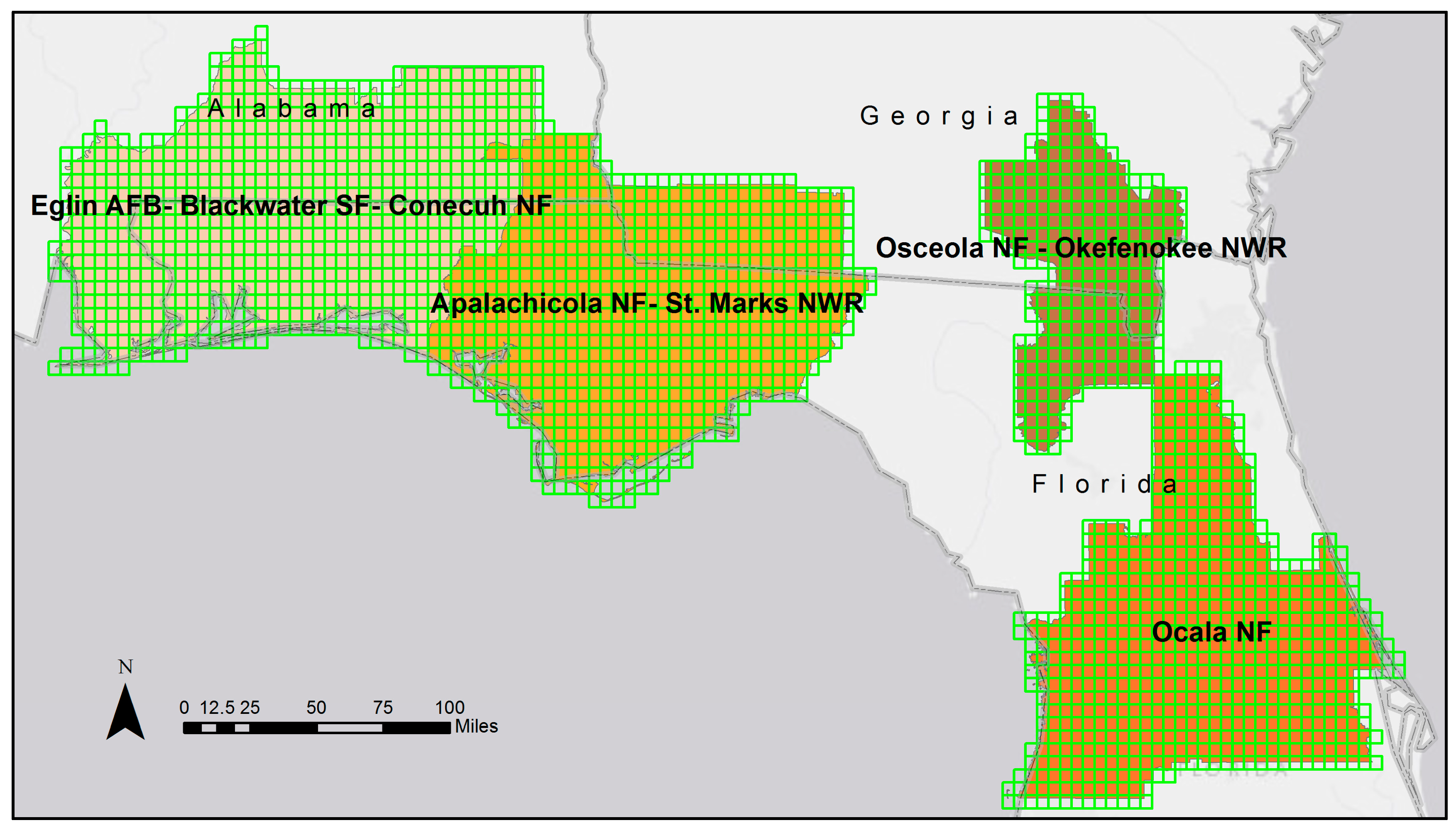
2.1. Study Area

Our study area consisted of four significant geographic areas (SGAs) in the southeastern United States delineated in the Range-Wide Conservation Plan for Longleaf Pine [27] (Figure 1). These areas have been targeted for focused longleaf pine (Pinus palustris) ecosystem restoration due to the existence of remnant longleaf pine and sites suitable for restoration, as well as the desire by land managers and stakeholders to restore longleaf ecosystems to these areas. Longleaf ecosystems are some of the most critically endangered ecosystems in the world [28]. What remains of these once dominant forests supports many rare plants and animals and provides refuge for threatened and endangered species [29].

2.2. Methods Overview

In addition to the NLCD, currently available land cover classification products in this study area include the Cooperative Land Cover Dataset (CLCD) [30] and Condition Class for Management (CCM) [31] map from Florida Natural Areas Inventory (FNAI) (Figure 2). The CLCD and CCM are vector and raster-based maps that provide fewer cover types than NLCD and are more directly tailored to longleaf pine, but only partially cover our study area. These land cover datasets, similar to NLCD, have a medium spatial resolution of 30 m to 100 m. The land cover classes at this medium resolution tend to be broad amalgams of the underlying vegetation that provide limited ability to prioritize areas for longleaf restoration or describe forest structure and composition at the stand scale.
To describe land cover at fine spatial resolutions, we created probabilistic land cover classification surfaces using United States Department of Agriculture (USDA) National Agricultural Imagery Program (NAIP) aerial photographic imagery that has a spatial resolution of 1 m [32]. Imagery like NAIP provides information with the fine spatial resolution needed to inform planning and prioritization, but must be translated into condition classes that are relevant to specific applications by conservation planners and stakeholders.
Our classification approach follows the recommendation of Hogland et al. [24] to produce probabilistic classification outputs from a combination of remotely sensed data and classification information (Figure 3). A series of softmax neural network (SNN) models was produced that links the principal components of NAIP spectral and texture values with a sample of visually interpreted points to produce 1 m probabilistic surfaces for 13 different visually distinct land cover classes (Table 1).
Due to state level differences in the base NAIP imagery, different models were produced for each of the three states in our study area (Alabama, Georgia, and Florida; Figure 1). Digital number (DN) values for each of the four NAIP bands were combined with standard deviation and grey level co-occurrence matrix (GLCM) values in singular vector decomposition principal component analysis (PCA) to reduce the dimensionality of the data and quantify patterns within the NAIP imagery [33]. The first six principle components of the PCA were used as predictor variables in our classification models. Sample points were visually classified in each state and combined with the PCA values to train SNN models. The SNN models for each state were then applied to produce probabilistic land cover classification surfaces for each of the four SGA. All analyses were performed using the RMRS Raster Utility toolbar [34] and ESRI’s ArcGIS geographic information system (GIS). To facilitate the tabular, spatial, statistical, and GIS analyses performed, we developed a suite of spatial modeling tools that take advantage of Function Modeling [24,35,36] and parallel processing. These tools work within ESRI’s GIS and are available for free download [34]. The remainder of this section describes in more detail the datasets and procedures used in this study.

2.3. Imagery and Data

We chose NAIP as our base imagery because of its fine spatial resolution, its complete coverage over the conterminous United States, and the fact that it is freely available for download [37]. We acquired NAIP color-infrared imagery flown in the year 2013 in Alabama, Georgia and Florida within our study area. NAIP color-infrared imagery consists of four 8-bit spectral bands (red, green, blue and near-infrared (NIR)) at 1 m spatial resolution. NAIP imagery within our SGAs was primarily collected from August to November of 2013 with parts of the Ocala SGA collected in May of 2013. Our 2013 NAIP imagery was acquired from aircraft using digital cameras and was mosaicked and separated into digital orthophoto quarter quad tiles (DOQQs) that are roughly 7 km east to west and 8 km north to south [32]. Our study area included 1674 DOQQ in Florida, 1008 in Georgia, and 537 in Alabama, totaling 3219 DOQQ (Figure 1). Each state’s tiles were mosaicked together on the fly in ESRI ArcMap as a mosaic raster dataset, which allowed us to refer to each state mosaic as a single raster for our analysis.
One major challenge to using fine resolution imagery like NAIP for a large geographic extent is the large amount of data, which can be unwieldy and time consuming to process [38]. Studies that have used NAIP imagery at large extents have addressed this challenge by limiting classification to a small number of classes that address specific land cover questions [11] in combination with the use of specialized computer hardware [10]. However, due to recent advances in image analysis software, we are now able to conduct broad extent fine resolution land cover classification using standard computer hardware more efficiently than was previously possible [34]. Specifically, the RMRS Raster Utility toolbar, and its associated ESRI ArcGIS add-in, uses function modeling, batch processing, advanced statistical models, and parallel processing to efficiently produce predictive models and surface outputs for big data applications [36].

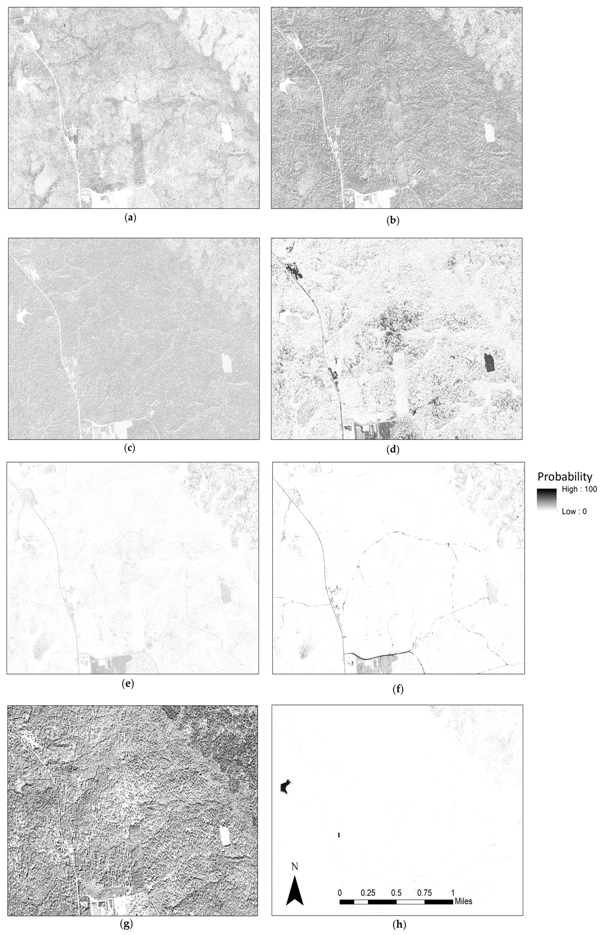
2.4. Predictive Surfaces

In addition to the NAIP spectral information, two texture variables were derived from each NAIP band in a 3 by 3 moving window to quantify the texture values of the cell’s immediate neighbors. Other moving window sizes, such as 4 × 4 and 5 × 5, were tested but added little to no significant textural information while increasing the complexity of the model and decreasing the model’s efficiency. Texture was quantified using a first-order standard deviation and a second order horizontal contrast gray level co-occurrence matrix (GLCM) for each of the four NAIP bands [39]. The textural measurements combined with the spectral values of the NAIP bands comprise the twelve bands that we used in our principal component analysis for each state. PCAs were performed for all data in each state using random samples of 20,859 cells in Alabama, 23,411 cells in Georgia, and 65,730 cells in Florida. Using the PCA models, we transformed the 12 bands derived from NAIP into principal component raster surfaces rescaled to values between 0 and 255. The top six principle components were used as predictive variables in our SNN models.

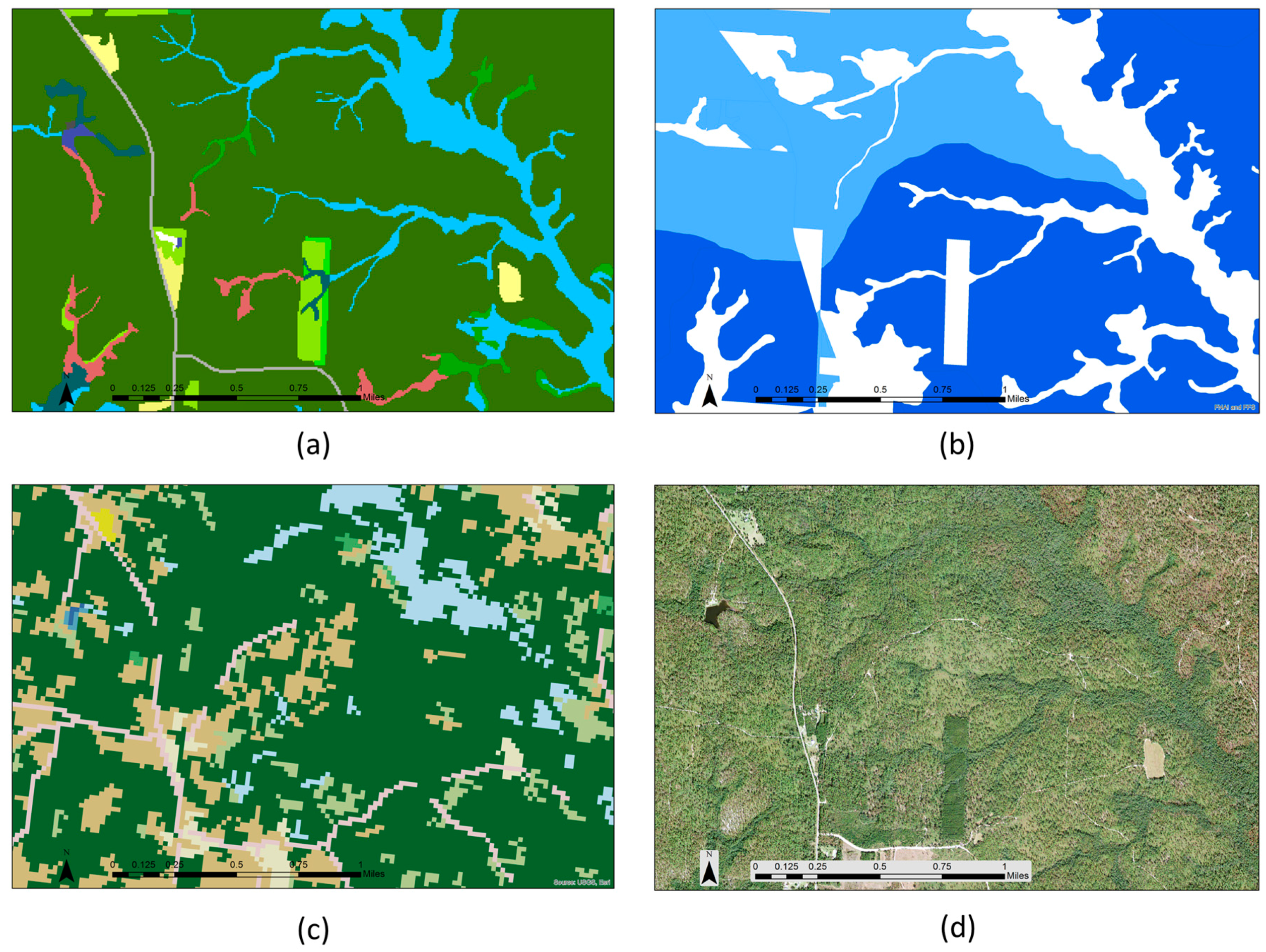
2.5. Classified Samples

The other input into the SNN models was a sample of visually interpreted locations. We randomly selected 3712 locations within our study area and digitized them as points, with 1640 points in Florida, 1083 in Alabama and 989 in Georgia. Sample points were visually classified into 13 land cover classes (Table 1) by an analyst for a 3 by 3 cell area surrounding the point location. The determination of the classes in Table 1 was driven by the imagery (classes must be visually distinct to a human classifier on NAIP, including the NIR band) and by the project requirements focused on identification of classes relevant to longleaf pine management and conservation. Some classes were easily identifiable including water, bare ground and pavement. Other classes were subdivided. For example, grass was subdivided into green and dry (dormant) grass, due to noticeably different spectral presentation. The dark, light and grey tree crown classes correspond to coniferous, deciduous, and senesced deciduous or dead trees, respectively. Each sample point’s spatial coordinates were used to extract the coincident values from the first six principal component surfaces and those values were appended to our visually classified points. SNN models were then developed to predict the probability of a cell being a specific class based on the principal component values derived from the NAIP imagery at that point.

2.6. Modeling

We chose to use SNN classification because it employs a machine learning technique that offers several advantages for use in land cover classifications. Specifically, neural networks are non-parametric and as such they do not assume known distributions of explanatory variables. The softmax function links the neurons in the neural network and produces probabilistic output values, which have been found to be more descriptive and flexible for land cover mapping than discriminant classification outputs [24,40]. Similar to various probabilistic multiclass classification methods, including multinomial logistic regression, SNN probabilistic outputs are themselves a per-cell estimation of the mean class probability [24]. This allows for easy estimates of model error for any subsequent rules that may be applied to a cell.
The classified points and their coincident principle component values were used to train a SNN model for each of the three states within our study area. We applied the SNN models to our principle component surfaces to create three 13 band raster surfaces that estimate the probability of a cell being each of the 13 land cover classes. The outputs were rescaled to integer values between 0 and 100, and saved as a 13-band unsigned 8-bit ERDAS Imagine (.img) file.

3. Results

3.1. PCA

To minimize the number of dimensions used in our modeling stage, we performed a PCA using NAIP spectral values and texture variables. In total we were able to reduce the dimensionality of the NAIP data and texture derivatives from 12 bands to 6. The top six principle components explained between 92% and 94% of the variation from our twelve input variables (Table 2). There were some common trends in all three PCA eigen vectors. The first two components emphasized red, blue and NIR GLCM contrast values, as well as the green band spectral value. The third component emphasized the green band spectral value along with the NIR spectral value, the red band GLCM value, and to a lesser extent the green and blue band standard deviation values. These three principal components accounted for approximately 78% of the variation in the data in all three PCAs. The remaining components emphasized standard deviation and horizontal GLCM contrast, as well as the NIR spectral value.
A total of 3219 six band principal component raster surfaces were created, corresponding to the number of DOQQ tiles covering our study area. NAIP DOQQ tiles were separated into mosaics by state. Each state was processed separately using a state specific PCA model. Processing time to create the principle component rasters was approximately 168 h (1 week). Rasters were processed in parallel across 16 logical cores on one computer using solid state drives and two 3.50 GHz Intel I7 processors. This amounted to roughly 40 min of processing time for each NAIP DOQQ.

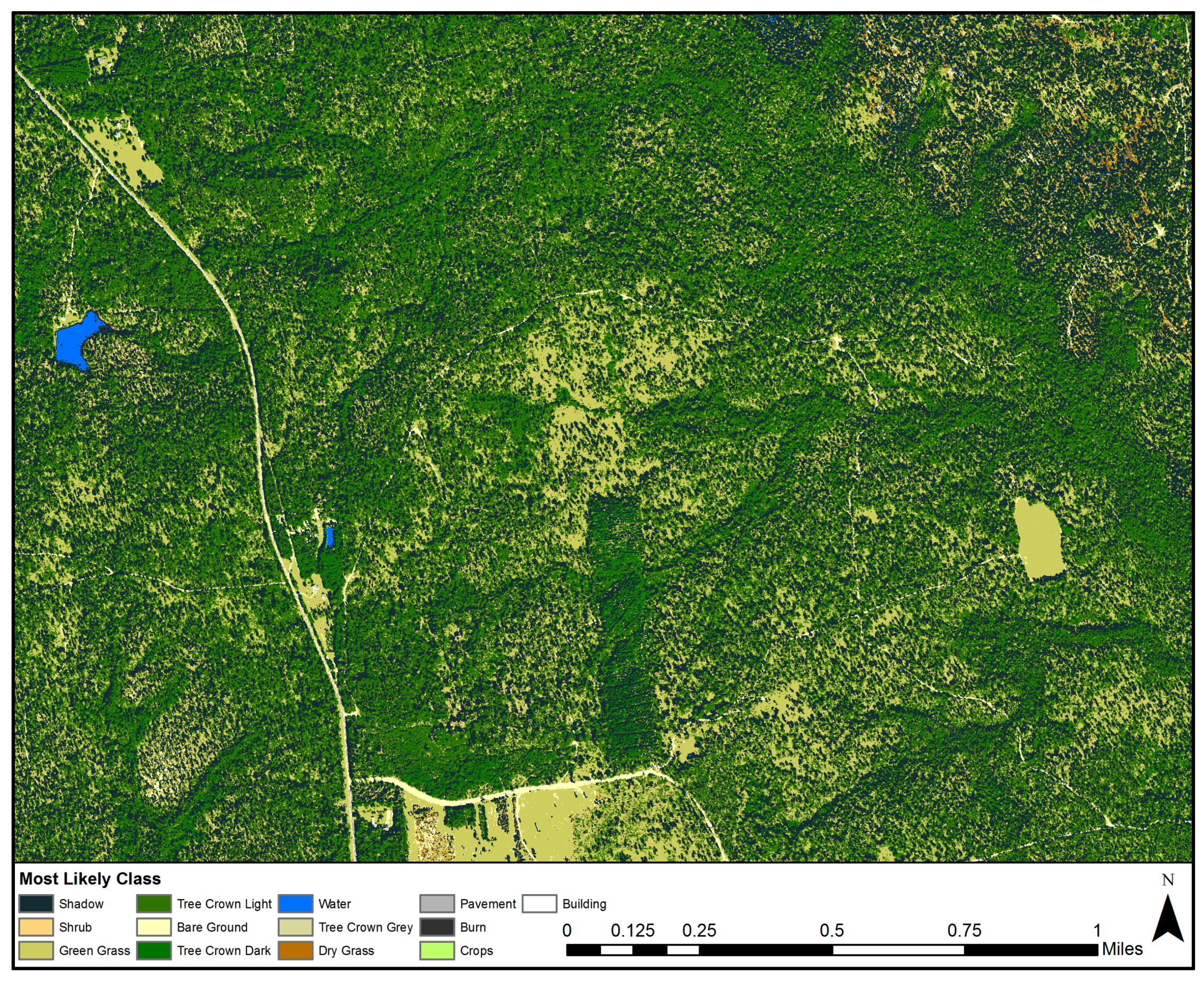
3.2. Modeled Outputs
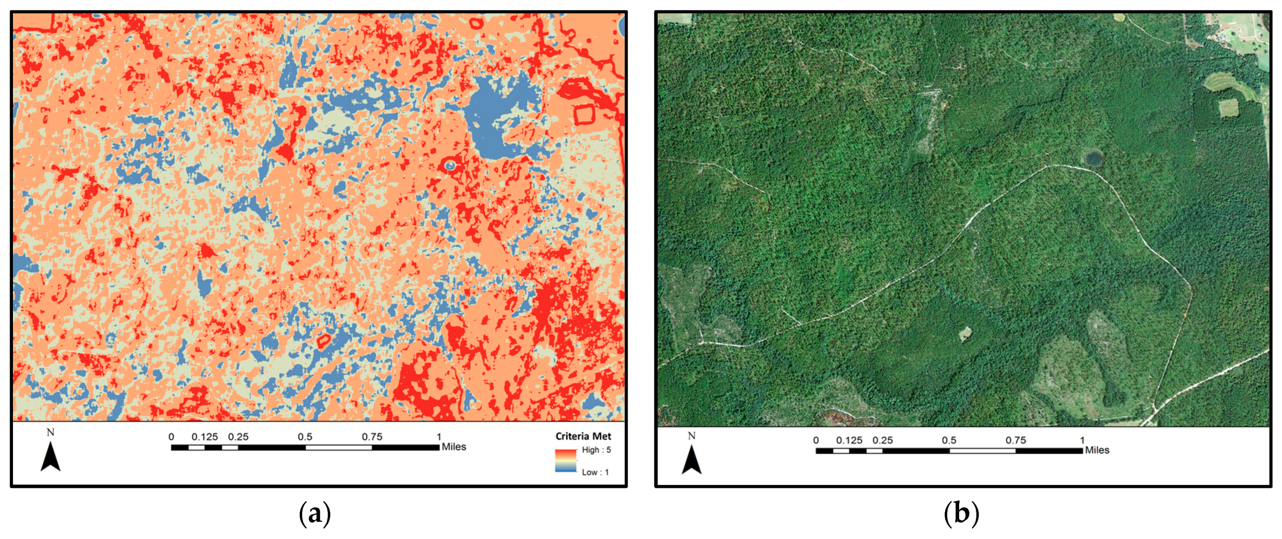
Using the values from the first six principal components and the sample of visually identified classes, we created three SNN models, one for each state within our study area. We used the average error (the difference between the training data values and the modelled values) in modeled probability to assess model fit. The average error of our three models ranged from 8.9% to 9.3% (Table 3). Using these models, and each state’s previously generated principle component mosaic, we built multiband probabilistic raster surfaces (13 bands each) for the extent of each DOQQ tile within a state, estimating the probability of each class for every raster cell (Figure 4). Probabilistic raster surfaces were then mosaicked together for each state. This process took approximately 40 min per DOQQ tile, running in parallel across 16 logical cores on a single computer. Total processing time for our entire study area was roughly 6 days.
The ability of the probabilistic land cover classifications to differentiate between cover classes is visually demonstrated in Figure 4, where darker shades indicate higher probabilities and lighter shades indicate lower probability. The vertical strip in the bottom middle of the image’s extent is a pine plantation and is apparent in the “tree crown dark” band, which is our coniferous cover class (Figure 4a) and its inverse in the “tree crown light” band, which is our deciduous cover class (Figure 4b). In a forested landscape such as this one, the shadow class (Figure 4h) is widespread and closely tied to shadows cast by trees, but has low probability in the fields and bare ground areas. The shrub band (Figure 4c) looks washed out because of the overall low probabilities of shrubs across the area. Distinct features are discernable in several cover classes: fields are distinguishable in the grass bands (Figure 4d,e), roads in the bare ground band (Figure 4f), and the two ponds within the figure’s extent appear as the only dark areas in the water band in Figure 4h. The dark areas of higher probabilities that compose these features are visual evidence of the model’s classification ability. Comparing these probabilistic classification outputs to the previously available land cover classifications in Figure 2 over the same extent makes the advantage of fine spatial resolution classification visually apparent.
The final raster outputs were 1.25 terabytes in total size at 1 m resolution. To facilitate use and distribution of this land cover classification we aggregated and resampled the 1 m outputs to a spatial resolution of 10 m. The aggregation routine calculated the average class probability for each land cover class within 100 square meters (100 cells in a 10 × 10 moving window). The resulting aggregation can be interpreted as the proportion of area each class occupies within that area. Final land cover outputs at both the 1 m and 10 m resolution were re-projected to Albers equal-area conic projection to facilitate accurate area estimates. The 10 m aggregate land cover classification products, along with all the products from the Longleaf Mapping Project, are available online [41].

3.3. Example of Use

The probabilistic land cover classification outputs in this study were developed to help identify and prioritize sites suitable for longleaf pine restoration. To demonstrate this application, we produced a simple set of rules that use cover percent to identify open pine stands (i.e., pine with large trees widely spaced with vegetative understory) and applied those rules to our land cover outputs to generate a conservation prioritization classification. Because our forest cover classifications do not distinguish between coniferous species, we were unable to directly locate longleaf pine cover explicitly. However, we did identify open pine stand characteristics that are typical of longleaf pine stands using our outputs [42]. First, we ran a continuous focal analysis on our land cover classification at the 1 m resolution. The focal analysis assigned the mean values of all cells within a 30 by 30 cell moving window to the central cell for each land cover class. The focal analysis allowed us to identify stand size areas and smooth the outputs while maintaining the 1 m spatial resolution. Then we applied five criteria to our focal analysis that identify open pine stands: pine cover between 3% and 30%, shrub plus grass cover greater than 20%, crop cover less than 20%, building plus pavement cover less than 20%; and water cover less than 25%. The pine and shrub/grass criteria are the primary characteristics associated with open pine stands, while the other three criteria were included to eliminate water bodies, urban areas, and croplands. The resulting classification is visualized in Figure 5.
Areas where all five criteria are met are defined as open pine stands. These criteria were effective at identifying areas of open pine stands, as seen in the bottom right of Figure 5, and in patches throughout. While the vast majority of areas within this example identify valid restoration sites, some areas that have forest and grass fields on either side of a road also meet the specified criteria, for example the top right corner of Figure 5. Fortunately, these areas are easily identified and can be quickly removed as potential restoration sites. This example illustrates that fine resolution land cover classification outputs alone can be used to identify and prioritize longleaf restoration sites based on established criteria. Moreover, they could be used as part of a more complex prioritization method, which might include spatial estimates of tree basal area and stand density, or ancillary data such as road layers, parcel ownership maps and digital elevation models (DEM).

4. Discussion

This study builds on previous work to demonstrate an adaptable method for overcoming the previously existing barriers to using fine resolution land cover classifications across a broad extent. In addition, our use of probabilistic classifications illustrates the adaptable nature of these types of classifiers and how these surfaces can inform multiple analyses. The software tools used to conduct the analysis make producing probabilistic land cover classifications of this resolution and extent obtainable for a wider audience by reducing processing, programming and memory requirements.
Our methodology efficiently produced probabilistic land cover surfaces at 1 m resolution across 11.6 million hectares (28.8 million acres) with less than 10% average error in modeled probability. The probabilistic surfaces can have various user defined rules applied in subsequent analysis such as an MLC rule (Figure 6) to address questions related to where classes are located, but are not limited to just one rule. This provides stakeholders with the flexibility needed to emphasize different characteristics of longleaf pine habitat in restoration planning. Due to the large extent, fine spatial resolution, and adaptability of these probabilistic land cover surfaces, multiple organizations can use these datasets as a common source of information for working to restore longleaf habitat in the region, even if those organizations use the data differently.
There were challenges unique to using NAIP imagery as a base predictor dataset. NAIP imagery is processed into a state-wide mosaic that contain seamlines. These seamlines are an artifact of when and how NAIP images were collected and processed. To cosmetically adjust differences in DN values due to acquisition times and processing, NAIP uses a color balanced routine which alters spectral information in the overlapping regions of images [17,32]. These aspects of acquisition and processing can increase the classification error of models built using this imagery. Because of how NAIP imagery is acquired and processed, we saw slight distortion of our outputs around the edges of the flight lines, which is likely an artifact of NAIP’s color balancing process. These challenges could be avoided by using different base imagery in this classification methodology, such as IKONOS or WorldView, however, these data can be expensive to obtain and would require additional image normalization.
Future classification studies using data from multiple years can add a temporal dimension to the analysis, allowing for land cover change studies at this high resolution. In the case of NAIP, this is facilitated by relatively frequent (2–3 year) return intervals. Ancillary inputs, such as DEM, Lidar data, or local high resolution spectral data, such as drone imagery, could be integrated into this methodology to improve specific class estimates and the downstream products that describe and map useful landscape characteristics. While our work has focused on spatial analysis for forest planning, restoration and management, the same methods can be used for land cover classification in many fields such as agriculture, wildlife management, and urban planning.
Datasets generated using this approach have a wide range of applications. For example, some forest condition class rules require shrub and grass percent cover thresholds to meet desired conditions [42]. Raster surfaces like ours can be easily queried to find locations across landscapes meeting those requirements. Additionally, classification rules such as MLC can be applied to the probabilistic surfaces to create hard classification. Land cover surfaces can be queried to rank areas based on certain characteristics, such as the percent cover of deciduous trees, or in combination with other classes in various weighting schema and ancillary spatial data. Combined with other datasets, such as land ownership data, stakeholders can compare outcomes and efficiencies of various prioritization strategies across large landscapes.

5. Conclusions

This project demonstrated a methodology to create a regional 1 m resolution probabilistic land cover classification with low average error outputs using standard computing hardware, ESRI GIS software and newly developed open source software. The fine resolution of the outputs provides land cover information at a resolution that is appropriate for use at the operational scale, such as prioritizing silvicultural treatments on specific ownerships and directing operations within individual forest stands. The probabilistic outputs are more flexible than hard classification outputs and can be used to derive many other data products for land management. Variables such as percent cover, forest composition, impervious surfaces, forested and non-forested land area, and the location of specific classes within any area can be quickly evaluated using a probabilistic land cover classification dataset. The low resource requirements and relatively quick processing time allows for low cost experimentation and provides a powerful new analytical tool for practitioners.

Acknowledgments

This work was funded by the United States Department of Agriculture (USDA), US Forest Service (State and Private Forestry, Region 8 and Rocky Mountain Research Station), the National Fish and Wildlife Foundation award number 50661 through the Longleaf Alliance, and by the USDA Agriculture and Food Research Initiative Competitive award no. 2013-68005-21298.

Author Contributions

Joseph St. Peter was the primary author of the manuscript and the technical lead in performing spatial analyses and developing raster surfaces. John Hogland proposed and built the RMRS Raster Utility software used in this study. He also developed the SNN models, designed the case study and contributed to the writing of the manuscript. Nathaniel Anderson provided project oversight and contributed to writing portions of the manuscript. Jason Drake and Paul Medley evaluated outputs and contributed to writing portions of the manuscript.

Conflicts of Interest

The authors declare no conflict of interest.

References

  1. Gao, J. Digital Analysis of Remotely Sensed Imagery, 1st ed.; McGraw-Hill: New York, NY, USA, 2009; pp. 249–290. [Google Scholar]
  2. Feddema, J.J.; Oleson, K.W.; Bonan, G.B.; Mearns, L.O.; Buja, L.E.; Meehl, G.A.; Washington, W.M. The Importance of Land-Cover Change in Simulating Future Climates. Science 2005, 310, 1674–1678. [Google Scholar] [CrossRef] [PubMed]
  3. Skidmore, A.K.; Pettorelli, N.; Coops, N.C.; Geller, G.N.; Hansen, M.; Lucas, R.; Mücher, C.A.; O’Connor, B.; Paganini, M.; Pereira, H.M.; et al. Agree on biodiversity metrics to track from space. Nature 2015, 523, 403–405. [Google Scholar] [CrossRef] [PubMed]
  4. Falcucci, A.; Maiorano, L.; Boitani, L. Changes in land-use/land-cover patterns in Italy and their implications for biodiversity conservation. Landsc. Ecol. 2007, 22, 617–631. [Google Scholar] [CrossRef]
  5. Mahiny, A.S.; Clarke, K.C. Guiding SLEUTH land-use/land-cover change modeling using multicriteria evaluation: Towards dynamic sustainable land-use planning. Environ. Plan. B Plan. Des. 2012, 39, 925–944. [Google Scholar] [CrossRef]
  6. McRoberts, R.E.; Tomppo, E.O. Remote sensing support for national forest inventories. Remote Sens. Environ. 2007, 110, 412–419. [Google Scholar] [CrossRef]
  7. Van Leeuwen, W.J.D. Monitoring the Effects of Forest Restoration Treatments on Post-Fire Vegetation Recovery with MODIS Multitemporal Data. Sensors 2008, 8, 2017–2042. [Google Scholar] [CrossRef] [PubMed]
  8. Koetz, B.; Morsdorf, F.; van der Linden, S.; Curt, T.; Allgöwer, B. Multi-source land cover classification for forest fire management based on imaging spectrometry and LiDAR data. For. Ecol. Manag. 2008, 256, 263–271. [Google Scholar] [CrossRef]
  9. Flamenco-Sandoval, A.; Ramos, M.M.; Masera, O.R. Assessing implications of land-use and land-cover change dynamics for conservation of a highly diverse tropical rain forest. Biol. Conserv. 2007, 138, 131–145. [Google Scholar] [CrossRef]
  10. Basu, S.; Ganguly, S.; Nemani, R.R.; Mukhopadhyay, S.; Zhang, G.; Milesi, C.; Michaelis, A.; Votava, P.; Dubayah, R.; Duncanson, L.; et al. A Semiautomated Probabilistic Framework for Tree-Cover Delineation From 1-m NAIP Imagery Using a High-Performance Computing Architecture. IEEE Trans. Geosci. Remote Sens. 2015, 53, 5690–5708. [Google Scholar] [CrossRef]
  11. Nagel, P.; Yuan, F. High-resolution Land Cover and Impervious Surface Classifications in the Twin Cities Metropolitan Area with NAIP Imagery. Photogramm. Eng. Remote Sens. 2016, 82, 63–71. [Google Scholar] [CrossRef]
  12. Forester, J.D.; Ives, A.R.; Turner, M.G.; Anderson, D.P.; Fortin, D.; Beyer, H.L.; Smith, D.W.; Boyce, M.S. State-space models link elk movement patterns to landscape characteristics in Yellowstone National Park. Ecol. Monogr. 2007, 77, 285–299. [Google Scholar] [CrossRef]
  13. Homer, C.G.; Dewitz, J.A.; Yang, L.; Jin, S.; Danielson, P.; Xian, G.; Coulston, J.; Herold, N.D.; Wickham, J.D.; Megown, K. Completion of the 2011 National Land Cover Database for the conterminous United States—Representing a decade of land cover change information. Photogramm. Eng. Remote Sens. 2015, 81, 345–354. [Google Scholar]
  14. Lu, D.; Weng, Q. A survey of image classification methods and techniques for improving classification performance. Int. J. Remote Sens. 2007, 28, 823–870. [Google Scholar] [CrossRef]
  15. Woods, B.; Clymer, B.; Heverhagen, J.; Knopp, M.; Saltz, J.; Kurc, T. Parallel four-dimensional Haralick texture analysis for disk-resident image datasets. Concurr. Comput. 2007, 19, 65–87. [Google Scholar] [CrossRef]
  16. Kotsiantis, S.B. Supervised Machine Learning: A Review of Classification Techniques. In Emerging Artificial Intelligence Applications in Computer Engineering, 1st ed.; Maglogiannis, I., Karpouzis, K., Wallace, B.A., Soldatos, J., Eds.; IOS Press: Amsterdam, The Netherlands, 2007; pp. 3–25. [Google Scholar]
  17. Hayes, M.M.; Miller, S.N.; Murphy, M.A. High-resolution landcover classification using Random Forest. Remote Sens. Lett. 2014, 5, 112–121. [Google Scholar] [CrossRef]
  18. Civco, D.L. Artificial neural networks for land-cover classification and mapping. Int. J. Geogr. Inf. Syst. 1993, 7, 173–186. [Google Scholar] [CrossRef]
  19. Huang, C.; Davis, L.S.; Townshend, J.R.G. An assessment of support vector machines for land cover classification. Int. J. Remote Sens. 2002, 23, 725–749. [Google Scholar] [CrossRef]
  20. Cleve, C.; Kelly, M.; Kearns, F.R.; Moritz, M. Classification of the wildland-urban interface: A comparison of pixel- and object-based classifications using high-resolution aerial photography. Comput. Environ. Urban Syst. 2008, 32, 317–326. [Google Scholar] [CrossRef]
  21. Hogland, J.S.; Anderson, N.M.; Chung, W.; Wells, L. Estimating forest characteristics using NAIP imagery and ArcObjects. In Proceedings of the 2014 ESRI Users Conference, San Diego, CA, USA, 14–18 July 2014; Available online: http://proceedings.esri.com/library/userconf/proc14/papers/155_181.pdf (accessed on 16 January 2018).
  22. Hogland, J.S.; Anderson, N.M. Estimating FIA plot characteristics using NAIP imagery, function modeling, and the RMRS raster utility coding library. In Proceedings of the New Directions in Inventory Techniques and Applications: Forest Inventory and Analysis (FIA) Symposium, Portland, OR, USA, 8–10 December 2015; U.S. Department of Agriculture, Forest Service, Pacific Northwest Research Station: Washington, DC, USA, 2015; pp. 340–344. [Google Scholar]
  23. Rodriguez-Galiano, V.F.; Chica-Olmo, M.; Abarca-Hernandez, F.; Atkinson, P.M.; Jeganathan, C. Random Forest classification of Mediterranean land cover using multi-seasonal imagery and multi-seasonal texture. Remote Sens. Environ. 2012, 121, 93–107. [Google Scholar] [CrossRef]
  24. Hogland, J.; Billor, N.; Anderson, N. Comparison of standard maximum likelihood classification and polytomous logistic regression used in remote sensing. Eur. J. Remote Sens. 2013, 46, 623–640. [Google Scholar] [CrossRef]
  25. Foody, G.M. Fuzzy modeling of vegetation from remotely sensed imagery. Ecol. Model. 1996, 85, 3–12. [Google Scholar] [CrossRef]
  26. Land Cover Data Project. Available online: http://chesapeakeconservancy.org/conservation-innovation-center/high-resolution-data/land-cover-data-project/ (accessed on 7 November 2017).
  27. America’s Longleaf. 2009 Range-Wide Conservation Plan for Longleaf. Available online: http://www.americaslongleaf.org/media/86/conservation_plan.pdf (accessed on 12 May 2015).
  28. Noss, R.; LaRoe, E.; Scott, J. Endangered Ecosystems of the United States: A Preliminary Assessment of Loss and Degradation; Biological Report 28; National Biological Service: Washington, DC, USA, 1995. [Google Scholar]
  29. Oswalt, C.M.; Cooper, J.; Brockway, D.G.; Brooks, H.W.; Walker, J.L.; Connor, K.F.; Oswalt, S.N.; Conner, R.C. History and Current Condition of Longleaf Pine in the Southern United States; General Technical Report SRS-166; U.S. Department of Agriculture Forest Service, Southern Research Station: Ashville, NC, USA, 2012; 51p.
  30. Cooperative Land Cover, Version 3.2. Published October 2016. Available online: http://myfwc.com/research/gis/applications/articles/cooperative-land-cover/ (accessed on 16 January 2018).
  31. LPEGDB Version 3 Summary Report—Florida Natural Areas Inventory. Available online: http://www.fnai.org/PDF/LPEGDB_v3_Summary_Report_Sep_2015.pdf (accessed on 16 January 2018).
  32. National Agriculture Imagery Program (NAIP) Information Sheet. Available online: http://www.fsa.usda.gov/Internet/FSA_File/naip_info_sheet_2013.pdf (accessed on 14 May 2014).
  33. Wold, S.; Esbensen, K.; Geladi, P. Principal Component Analysis. Chemom. Intell. Lab. Syst. 1987, 2, 37–52. [Google Scholar] [CrossRef]
  34. RMRS Raster Utility. Available online: http://www.fs.fed.us/rm/raster-utility (accessed on 24 January 2018).
  35. Hogland, J.; Anderson, N. Improved analyses using function datasets and statistical modeling. In Proceedings of the 2014 ESRI Users Conference, San Diego, CA, USA, 14–18 July 2014; Environmental Systems Research Institute: Redlands, CA, USA, 2014. [Google Scholar]
  36. Hogland, J.; Anderson, N. Function Modeling Improves the Efficiency of Spatial Modeling Using Big Data from Remote Sensing. Big Data Cogn. Comput. 2017, 1, 1–14. [Google Scholar] [CrossRef]
  37. United States Geological Survey File Transfer Protocol [USGS FTP] (2016) Staged NAIP. Available online: ftp://rockyftp.cr.usgs.gov/vdelivery/Datasets/Staged/NAIP/ (accessed on 16 September 2016).
  38. Maxwell, A.E.; Warner, T.A.; Vanderbilt, B.C.; Ramezan, C.A. Land Cover Classification and Feature Extraction from National Agriculture Imagery Program (NAIP) Orthoimagery: A Review. Photogramm. Eng. Remote Sens. 2017, 83, 737–747. [Google Scholar] [CrossRef]
  39. Haralick, R.M.; Shanmugam, K.; Dinstein, I. Textural Features for Image Classification. IEEE Trans. Syst. Man Cybern. 1973, SMC-3, 610–621. [Google Scholar] [CrossRef]
  40. Bishop, C.M. Pattern Recognition and Machine Learning; Springer Science+Business Media, LLC: New York, NY, USA, 2006; pp. 179–224. [Google Scholar]
  41. Hogland, J.; St. Peter, J.; Anderson, N. Raster Surfaces Created from the Longleaf Mapping Project. Fort Collins, CO: Forest Service Research Data Archive. 2017. Available online: https://doi.org/10.2737/RDS-2017-0014 (accessed on 16 January 2018).
  42. America’s Longleaf. 2014 Longleaf Pine Maintenance Condition Class Definitions. Available online: http://www.americaslongleaf.org/media/14299/final-lpc-maintenance-condition-class-metrics-oct-2014-high-res.pdf (accessed on 2 May 2016).
Figure 1. The four significant geographic areas (SGA) that are included in our study area along with the grid of overlapping National Agriculture Imagery Program (NAIP) digital orthophoto quarter quad (DOQQ) tiles.
Ijgi 07 00107 g001
Figure 2. Sample images from available public land cover classification products in our study area: (a) Cooperative Land Cover dataset from Florida Natural Areas Inventory; (b) Condition Class for Maintenance of Longleaf dataset from Florida Natural Areas Inventory; (c) National Land Cover Dataset (2011); and (d) National Agricultural Imagery Program (2013), which is the imagery used in this study for probabilistic classification.
Ijgi 07 00107 g002
Figure 3. Flowchart of our classification methodology.
Ijgi 07 00107 g003
Figure 4. Comparison of probabilistic classification outputs: (a) ‘tree crown dark’ (our coniferous tree class); (b) tree crown light (our deciduous tree class); (c) shrub class; (d) green grass class; (e) dry grass class; (f) bare ground; (g) shadow class; (h) water class.
Ijgi 07 00107 g004
Figure 5. (a) Open pine areas prioritized for conservation based on percent cover within a 30 m window. Colors correspond to the number of criteria met. The criteria are: pine cover between 3–30%, shrub plus grass cover greater than 20%, crop cover less than 20%, building plus pavement cover less than 20%, and water cover less than 25%; (b) NAIP imagery for the same extent.
Ijgi 07 00107 g005
Figure 6. Example of a high-resolution land classification generated by applying a most likely class (MLC) rule to a 13 band probabilistic land cover classification.
Ijgi 07 00107 g006
Table 1. Land cover classes and descriptions.
ClassDescription
ShadowShadows associated with an object
PavementRoads, driveways, and other paved objects
BuildingBuildings
Tree Crown LightLight green trees usually broadleaf
Tree Crown DarkDark green trees usually coniferous
ShrubGreen shrub species
Green GrassGrowing grass
WaterLakes, ponds, streams and ocean
BurnRecently burned charred areas
Bare GroundExposed soil or rock
Tree Crown GreyGrey tree canopy usually senesced broadleaf
Dry GrassDormant grass
CropsPlatted or irrigated areas that did not have exposed soil
Table 2. Cumulative proportion of variation explained by each component for each state’s principal component analysis (PCA).
ComponentsAlabamaGeorgiaFlorida
139.84%36.45%42.08%
269.12%65.90%68.67%
377.95%76.43%77.58%
484.34%82.95%84.09%
589.65%88.20%89.85%
693.53%92.77%93.60%
795.69%95.34%95.69%
897.21%97.16%97.33%
998.38%98.23%98.46%
1099.20%99.15%99.31%
1199.64%99.61%99.67%
12100.00%100.00%100.00%
Table 3. Softmax neural network land cover model average error for each state.
StateModeled Average Error
Alabama9.1%
Florida9.3%
Georgia8.9%

