Exploring the Role of the Spatial Characteristics of Visible and Near-Infrared Reflectance in Predicting Soil Organic Carbon Density

Abstract

Soil organic carbon stock plays a key role in the global carbon cycle and the precision agriculture. Visible and near-infrared reflectance spectroscopy (VNIRS) can directly reflect the internal physical construction and chemical substances of soil. The partial least squares regression (PLSR) is a classical and highly commonly used model in constructing soil spectral models and predicting soil properties. Nevertheless, using PLSR alone may not consider soil as characterized by strong spatial heterogeneity and dependence. However, considering the spatial characteristics of soil can offer valuable spatial information to guarantee the prediction accuracy of soil spectral models. Thus, this study aims to construct a rapid and accurate soil spectral model in predicting soil organic carbon density (SOCD) with the aid of the spatial autocorrelation of soil spectral reflectance. A total of 231 topsoil samples (0–30 cm) were collected from the Jianghan Plain, Wuhan, China. The spectral reflectance (350–2500 nm) was used as auxiliary variable. A geographically-weighted regression (GWR) model was used to evaluate the potential improvement of SOCD prediction when the spatial information of the spectral features was considered. Results showed that: (1) The principal components extracted from PLSR have a strong relationship with the regression coefficients at the average sampling distance (300 m) based on the Moran’s I values. (2) The eigenvectors of the principal components exhibited strong relationships with the absorption spectral features, and the regression coefficients of GWR varied with the geographical locations. (3) GWR displayed a higher accuracy than that of PLSR in predicting the SOCD by VNIRS. This study aimed to help people realize the importance of the spatial characteristics of soil properties and their spectra. This work also introduced guidelines for the application of GWR in predicting soil properties by VNIRS.

1. Introduction

Soil is an important global reservoir for soil organic carbon (SOC), which plays a key role in the global carbon cycle [1]. Soil holds the largest terrestrial storage of organic carbon. Slight changes on soil organic carbon density (SOCD) can significantly influence the atmospheric CO₂ concentration and carbon balance. These effects further exacerbate the greenhouse effect and global climate change [2]. Furthermore, SOC is a measureable component of soil organic matter, which is an important source of soil nutrients. Soil organic matter is a complex mixture related to the physical, chemical, and biological soil fertilities. These fertilities determine the nutrient turnover, soil structure, soil moisture retention, and soil availability [3]. Hence, efficient and rapid methodologies are necessary to the understanding of the role of soils in the global C cycle and the monitoring of the change in SOCD in precision agriculture.

Numerous studies quantified the SOC stocks at a global scale and among different country regions. SOCD, as an important parameter used to calculate SOC stock, needs a series of soil measurements and complex experimental operations and field investigations [4,5]. The soil measurements entailed include the SOC, soil moisture content, gravel concentration, soil bulk density, and soil thickness. All of these experiments and investigations are time consuming, relatively expensive, and not adaptable to in situ determinations. The calculation accuracy of the SOC stock is also influenced by the density of the soil sampling points. Thus, simultaneously increasing the spatial resolution and enlarging the extent of conventional soil methods is a challenging task. Visible and near-infrared reflectance spectroscopy (VNIRS; 350–2500 nm) provides a valid alternative to conventional methods for the estimation of soil properties [6,7]. SOC stocks represent more important information than that of single SOC or soil organic matter concentrations in the global warming context. Even so, only a few studies successfully predicted SOCDs by VNIRS because SOCD is a composite soil attribute [8,9]. The SOCD is calculated by many other relevant soil properties, such as SOC, soil moisture, and soil bulk density. Consequently, the relationship of SOCD with visible and near-infrared reflectance (VNIR) spectral data is decreased. Many investigations showed that the relevant soil properties of SOCD can be successfully predicted by VNIRS. The distinct absorption features of soil organic matter or SOC are influenced by various chemical bonds (C–H, C–C, C=C, C–N, and O–H) in the VNIR regions [10,11]. Measuring soil bulk density, as another necessary parameter to calculate SOCD, needs considerable amount of time and labor. However, the soil bulk density is influenced with soil moisture and soil texture, which can be predicted by the VNIR spectral data [12,13]. Therefore, we hope the present study results can offer a theoretical basis for the feasible potential of VNIRS in predicting SOCD. This hypothesis should be investigated to save a considerable amount of time and avoid tedious experiments.

Partial least squares regression (PLSR), as a highly commonly used model, can solve the redundancy and multicollinearity of spectral reflectance. Thus, PLSR is frequently applied to determine the fundamental relationship between soil property and spectral reflectance [14,15]. Although PLSR excellently predicts soil properties by soil spectral reflectance, the method is a non-spatial regression model that has not covered well the spatial autocorrelation of soil properties [16]. Many studies showed that soil properties exhibit strong spatial heterogeneity and dependence because of the effects of social and natural environments [17,18]. VNIRS can reflect the physical constructions and chemical substances of soil; this technique can also determine the spatial characteristics of soil properties [7,19,20]. Nevertheless, most previous investigations used the traditional linear regression models (such as PLSR) to construct the soil spectral models. These investigations also utilized soil samples as independent variables and ignored the spatial characteristics of the soil properties. Hence, the prediction accuracy of the spectral models is influenced by the spatial autocorrelation and variation of the soil properties. The spatial autocorrelation of soil properties and VNIRS should be considered when constructing the soil spectral models, particularly, in the local study region, to improve the robustness of the spectral models [21,22].

Given that traditional non-spatial models do not consider the spatial characteristics of soil properties, some scholars used the spatial or geostatistical models to solve this issue [21,23]. Recently, the use of a local spatial regression method, called geographically-weighted regression (GWR), as an alternative in spatial modeling of environmental variables, has attracted the attention of environmental experts [24,25]. GWR is an extension of the traditional regression framework, which allows modeled coefficients of environmental covariates to vary at different locations [25]. The spatial relationships between the explanatory and explained variables can be evidently shown by the spatially varied correlation coefficients of GWR [26]. Thus, GWR can be used to explore the spatial variation relationships between the soil properties and the auxiliary variables in different geographical locations. GWR has been used to construct prediction models using environmental factors as auxiliary variables. Nevertheless, this method is seldom used in predicting soil properties through VNIRS [27,28]. In contrast to PLSR, GWR can capture the spatial variability of SOCD and its varied relationships with VNIR spectral reflectance. This achievement is due to the flexibility of GWR in modeling relationships over locations [29]. Consequently, the spatial autocorrelation of SOCD can be considered through the flexible bandwidths and the varied spatial weights in constructing the local spatial regression models. The non-stationarity of the influence degree between the VNIR spectral data and SOCD can be shown by the GWR coefficient maps in different geographical locations. Therefore, the potential of GWR in predicting soil properties by VNIR spectral reflectance should be explored. The necessity for spatial autocorrelation in constructing the soil spectral models should also be discussed.

The Jianghan Plain, located in the middle and south of Hubei Province, is an alluvial plain and an important food grain region in China. The rapid and accurate prediction of SOCD can help obtain further information on the status and change in soil fertility. A total of 231 top soil samples (0–30 cm) were collected from the Jianghan Plain. GWR was used to predict the SOCD by VNIRS, and PLSR was utilized as the reference model. The present study aimed to (1) determine the feasibility of predicting SOCD by VNIRS; (2) discuss the necessity of spatial autocorrelation in predicting SOCD by VNIRS; and (3) show the variable relationships among soil components, spectral reflectance, and SOCD.

2. Materials and Methods

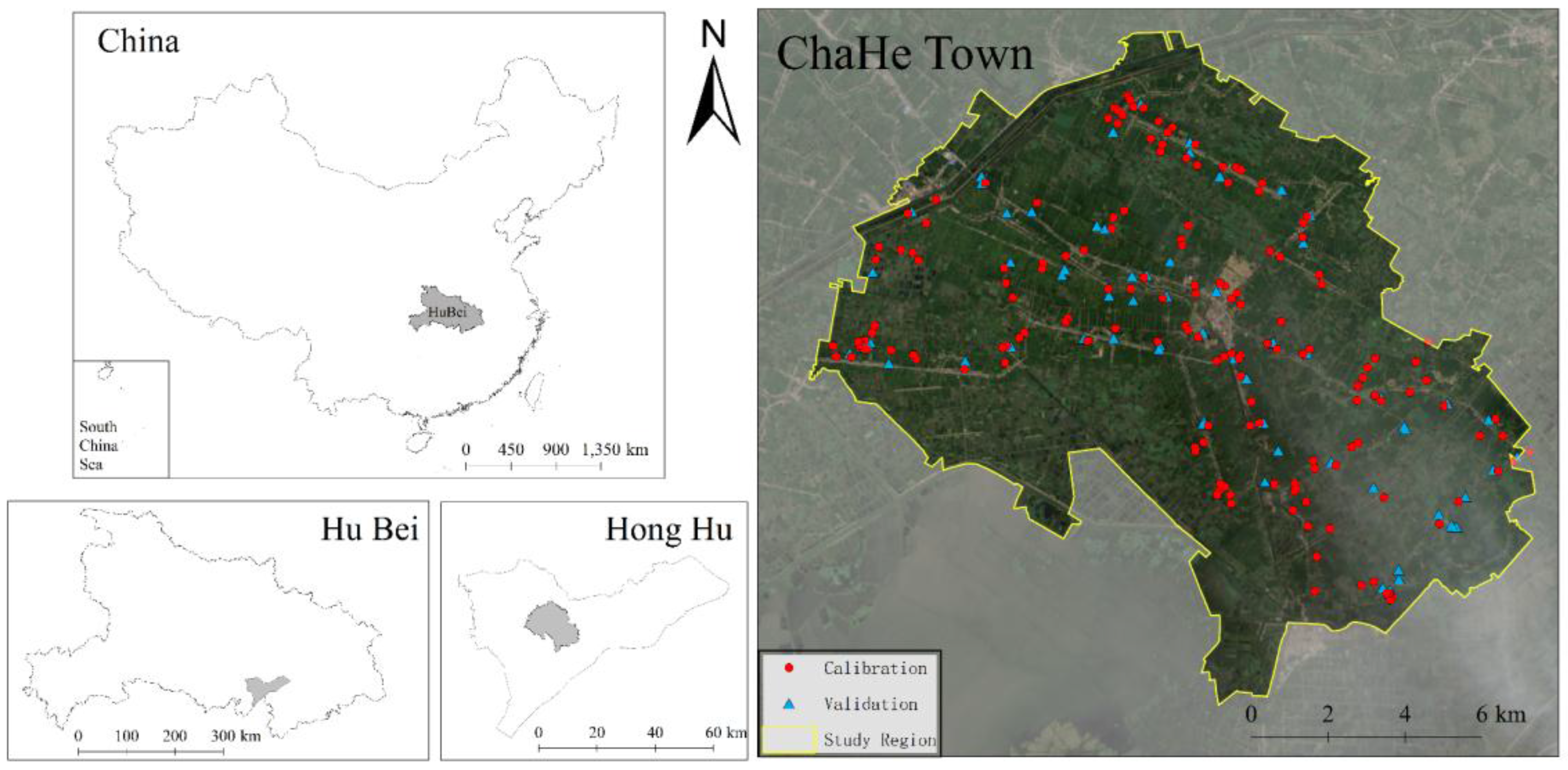
2.1. Study Area

Chahe Town, which is located at the center of Jianghan Plain (29.39°–30.12° N latitude, 113.7°–114.05° E longitude), was selected as the study region (Figure 1). The Jianghan Plain, an alluvial plain with main land use types of non-irrigated and paddy lands, is an important food grain region in China. Chahe Town experiences a subtropical humid monsoon climate with evident features of continental climate. The weather is relatively moderate with an annual average temperature of 16.6 °C. The rainfall is abundant with a mean annual precipitation of 1154 mm. The main soil parent materials of this study region are river alluvium and lacustrine deposits. This area is also appropriate and suitable for various crops. The soils are diverse and categorized into various Chinese soil taxonomy classifications [30], including paddy, moisture, dark-yellow–brown, and yellow–brown soils. Their approximate World Reference Base of Soil Resources classification are Stagnic Anthrosols, Eutyic Cambisols, Humic Cambisols, and Alfisol [31].

The geographical area of Chahe Town is approximately 153 km², and the elevation ranges from 2 m to 35 m. The geostatistical range of soil organic matter was 100–1000 m based on experiential knowledge [32]. A total of 231 topsoil samples (0–30 cm) were collected from the roads by the random sampling method in June 2013 to guarantee the full coverage of Chahe Town. The distances between each sampling site range from 100 m to 1459 m, and the shortest distance from the soil samples to the road is 100 m. For each soil sample, five soil subsamples taken within 1 m² were collected and thoroughly mixed to obtain a representative sample. The surface soils (0–30 cm) were collected after removing plants and debris covering the soil surface. The soil samples were first air dried in the laboratory at 20–25 °C for 14 days. Subsequently, the dried soil samples were gently crushed in a porcelain mortar to break down large aggregates and sieved using a 0.25 mm stainless-steel sieve. The sieved dry soil samples can remove the influence of the soil texture and the soil moisture, and then reflect the spectral characteristics of the soil samples. One part of the soil sample was used to measure the SOC in the laboratory. Another part was used to measure the VNIR spectral reflectance. Three parallel tests for each soil sample were processed to measure the SOC content through the potassium dichromate method [33,34]. A cutting ring with a volume of 100 cm³ was used to measure the weight of the wet soil. This test was repeated three times to calculate the mean value. At the same location, three aluminum specimen boxes were used to measure the soil moisture content [35]. The soil bulk density was calculated on the basis of the weight of the wet soil and the soil moisture using the Pedotransfer function developed by Calhoun, et al. [36] (R² = 0.56).

The SOCD content was calculated in accordance with the function of Thompson and Kolka [37]:

$${\rho }_{\mathrm{SOC}}={\displaystyle \sum }_{i=1}^n\left(1-{\theta }_i\%\right)\times p_i\times C_i\times T_i/100,$$

(1)

where ${\rho }_{\mathrm{SOC}}$ is the SOCD (kg m⁻²) of the top soil (0–30 cm), i is the soil horizon (1, 2, 3, …, n), ${\theta }_i\%$ is the gravel concentration (>2 mm) in the ith horizon, $p_i$ is the soil bulk density of the rock-free soil in the ith horizon (g cm⁻³), $C_i$ is the SOC content (g kg⁻¹) measured by the potassium dichromate method, and T_i is the soil thickness (cm).

2.2. Laboratory Measurements and Spectral Pre-Processing

The spectral reflectance of soils was recorded in the VNIRS range (350 nm to 2500 nm) with spectral resolutions of 3 nm from 350 nm to 1000 nm and 10 nm from 1000 nm to 2500 nm using a ASD FieldSpec3 (Analytical Spectral Devices, Longmont, Colorado, USA) portable spectral radiometer (http://www.asdi.com). The spectral readings were acquired in 1 nm increments over the wavelength range. The soil sample was placed in a 10 cm diameter Petri dish at a thickness of approximately 15 mm. The spectra of the soil samples were recorded in a dark room with a 50 W halogen lamp as the light source that was positioned 0.3 m away from the samples with a 158° zenith angle; the optical probe was installed approximately 0.15 m above the sample [38]. The correction using a standardized white Spectralon panel with 100% reflectance was made before the first scan and after every 10 samples (http://www.labsphere.com/). The average value of 10 spectral measurements for each sample was calculated as the final spectral reflectance.

Given the variations in soil structural properties and working conditions of the spectroradiometer, the spectral reflectance inevitably exhibits many problems, including multicollinearity, random noise, baseline drift, and multiple scattering effect, which may affect the robustness and accuracy of the calibration models [14]. Therefore, spectral pre-processing was conducted during chemometric modeling. The robust principal component analysis method was used to detect and eliminate the outliers from the original datasets. The reflectance spectra were first reduced to 400 nm–2350 nm to eliminate the noise at the spectral edges. Then, the reflectance curves were smoothed to further eliminate noise with a moving window of 15 nm using the Savitzky–Golay smoothing method. The continuum removal technique was used to isolate particular absorption features in diffuse reflectance spectra. The continuum-removed spectrum of each group was obtained to highlight the spectral absorption features. Finally, standard normal variate was used as a typical example of scatter-corrective methods to remove, to some extent, the undesired scatter or particle-sized information from spectral reflectance [39]. These methods were implemented in the PLS toolbox (Version 7.9.3, Eigenvector Research, Inc., Wenatchee, WA, USA) operated in MATLAB^® (R2008a, MathWorks, Inc., Natick, MA, USA).

2.3. PLSR and GWR

PLSR is a modeling technique often used in chemometric and quantitative spectral analyses. PLSR is based on linear transition from a large number of original descriptors to a new variable space based on a small number of orthogonal factors [40]. The PLSR algorithm selects successive orthogonal factors that maximize the covariance between predictors (x spectra) and the response variable (y, e.g., SOCD data). The PLSR model contains a parsimonious set of factors and latent variables selected in a manner such that their correlations with the response variable are maximized. Additional details on the PLSR algorithm can be referred to the study of Harald and Paul [41]. The PLSR formulas were as follows:

$${\widehat{Z}}_{PLSR}\left(x_i,y_i\right)={\displaystyle \sum }_{k=0}^p{\widehat{\beta }}_k\times q_k\left(x_i,y_i\right), i=1,\dots ,n$$

(2)

$$q_k\left(x_i,y_i\right)={\displaystyle \sum }_{j=1}^m{l}_j^{\prime }\times X_j\left(x_i,y_i\right), i=1,\dots ,n$$

(3)

where ${\widehat{Z}}_{PLSR}\left(x_i,y_i\right)$ is the SOCD content at geographical location $\left(x_i,y_i\right)$ estimated by the $\mathrm{PLSR}$ model;$q_k\left(x_i,y_i\right)$ is the transferred components from the spectral reflectance of soil samples at location $\left(x_i,y_i\right)$ by PLSR, and no linear relationship exists between any two $q_k\left(x_i,y_i\right)$. ${\widehat{\beta }}_k$ comprises the estimated drift model coefficients in the PLSR model. p is the suitable number of principal components (PCs) transformed from PLSR. m is the total number of spectral wavelength. $l_j^{\prime }$ is the eigenvector in the PLSR model. Finally, $l_j^{\prime }\times l_j=1$, and $X_j\left(x_i,y_i\right)$ is the spectral reflectance of the soil sample. The PLSR was implemented using the PLS toolbox (Version 7.9.3, Eigenvector Research, Inc., Wenatchee, WA, USA) operated in MATLAB^® (R2008a, MathWorks, Inc., Natick, MA, USA).

In this paper, the PCs extracted from PLSR were used as the auxiliary variables of GWR. GWR extends the traditional regression framework by considering the geographical locations of parameters [24,42,43]. The GWR model can be expressed as follows:

$${\widehat{Z}}_{GWR}\left(x_i,y_i\right)={\beta }_0+{\displaystyle \sum }_{k=1}^p{\beta }_k\left(x_i,y_i\right)\times q_k\left(x_i,y_i\right)+\epsilon \left(x_i,y_i\right), i=1,\dots ,n$$

(4)

where ${\widehat{Z}}_{GWR}\left(x_i,y_i\right)$ is the SOCD content at the geographical location $\left(x_i,y_i\right)$; $q_k\left(x_i,y_i\right)$ is the PCs of spectral reflectance transformed by the PLSR model; ${\beta }_0$($x_i,y_i$) is the intercept of local GWR model at geographical location $\left(x_i,y_i\right)$; ${\beta }_k\left(x_i,y_i\right)$ are the coefficients of different components; p is the suitable number of PCs that will be used to construct the prediction models;$q_k\left(x_i,y_i\right)$ comprise the PCs transformed from the spectral reflectance of soil samples at location $\left(x_i,y_i\right)$ (Equation (3)); $\epsilon \left(x_i,y_i\right)$ is the error term generally assumed to be independent and normally distributed with zero means and constant variance ${\mathsf{\sigma }}^2$; and n is the total number of soil samples. The regression coefficients of this equation were estimated at each location. Data were used to fit the regression in accordance with their spatial locations. This action resulted in large weights to the points closest to the prediction location. Furthermore, GWR can determine the spatial variations of soil properties and spectral reflectance.

The optimal bandwidth allocation is the critical part in GWR. This study employed the corrected Akaike information criterion (AICc), which is fixed by the maximum likelihood principle, to determine the optimal bandwidth. Hurvich, et al. [44] used the AICc in selecting the smoothing parameters in nonparametric regressions. Brunsdon, Fotheringham, and Charlton [24] applied the AICc to select the bandwidth in GWR. AICc is calculated as follows:

$$\mathrm{AICc}=-2\ln L({\widehat{\theta }}_L,X)+2q$$

(5)

where ${\widehat{\theta }}_L$ is the maximum likelihood estimator and q is the number of unknown parameters. The greater the likelihood function is, the better the estimator. Thus, AICc with a minimum value indicates that the model is optimized. The GWR was implemented by the spatial statistics modules in ArcGIS (Version 10.4.1, Esri Inc., Redlands, CA, USA).

2.4. Model Evaluation

The accuracy of the models for each test was evaluated based on the validation dataset by calculating the root mean square error (RMSE) and R² of the calibration model (RMSE_C and R²_C) and the prediction model (RMSE_P and R²_P) and the ratio of percentage deviation (RPD) [45].

$$R^2=1-\frac{{{\displaystyle \sum }}_{i =1}^n{\left(y_i-{\widehat{y}}_i\right)}^2}{{{\displaystyle \sum }}_{i =1}^n{\left(y_i-\overline{y}\right)}^2}$$

(6)

$$\mathrm{RMSE}=\sqrt{\frac{1}{n}{\displaystyle \sum }_{i =1}^n{\left(y_i-{\widehat{y}}_i\right)}^2}$$

(7)

$$\mathrm{RPD}=\frac{\mathrm{SD}}{{\mathrm{RMSE}}_p}$$

(8)

where n is the sample number, $y_i$ is the measured value for the soil sample, ${\widehat{y}}_i$ is the predicted value, and $\overline{y}$ is the mean measure value.

The RPD is defined as the ratio of the standard deviation (SD) of the validation dataset and the RMSE_P, which indicates the predictive performance of the calibration models. RPD was interpreted by Chang et al. (2001) as follows: (1) good predictions when RPD > 2.0 and R² > 0.8; (2) predictions with potential when RPD = 1.4 to 2.0 and R² = 0.50 to 0.80; and (3) unreliable predictions when RPD < 1.4 and R² < 0.5.

3. Results

3.1. Basic Statistics of SOCD

A total of 231 soil samples (0.33–10.16 kg·m⁻²) were divided into a calibration dataset (n = 161, 70%; 0.33–10.16 kg·m⁻²) and a validation dataset (n = 70, 30%; 2.47–8.27 kg·m⁻²) on the basis of the Kennard–Stone method [46]. The calibration dataset showed a wider range (9.84 kg·m⁻²), a smaller minimum value (0.33 kg·m⁻²), and a larger maximum value (10.16 kg·m⁻²) than those of the validation dataset (5.80, 2.47, and 8.27 kg·m⁻², respectively) (

Table 1. Basic statistics of soil organic carbon density (SOCD), soil moisture and soil organic carbon in the entire, calibration, and validation datasets.

	Number	Range	Min	Max	Mean	SD	CV (%)	CS	CK
Calibration dataset (kg·m−2)	161	9.84	0.33	10.16	5.37	1.96	36.53%	0.12	−0.41
Validation dataset (kg·m−2)	70	5.80	2.47	8.27	4.81	1.62	33.65%	0.48	−0.79
Entire dataset (kg·m−2)	231	9.84	0.33	10.16	5.20	1.88	36.12%	0.25	−0.45
Soil moisture	231	1.70	0.07	1.77	0.38	0.02	4.26%	1.76	3.76
Soil Organic Carbon (g kg−1)	231	43.98	0.83	44.82	15.70	7.20	2.76%	0.81	0.65

Min: Minimum, Max: Maximum, SD: Standard deviation, CV: Coefficient variation, CS: Coefficient of skewness, CK: Coefficient of kurtosis.

). Consequently, the SOCD values of the validation dataset were included in the calibration dataset to ensure the accuracy of the classification. The mean values of the calibration, validation, and entire datasets were 5.37, 4.81, and 5.20 kg·m⁻² with a standard deviation of 1.96, 1.62, and 1.88 kg·m⁻², respectively. The basic statistics of the calibration and validation datasets were similar to those of the entire dataset. This similarity indicates that the calibration and validation datasets could effectively represent the entire dataset. The coefficient of variation (CV) was used to interpret the variability of soil attributes. Soil attributes were classified into most (CV > 35%), moderate (CV: 15–35%), and least (CV < 15%) variable classes as proposed by Buchmann [47]. The CV values of SOCD were 36.53%, 33.65%, and 36.12% for the calibration, validation, and entire datasets, respectively. The SOCD of the entire and calibration datasets exhibited a strong variation, whereas that of the validation dataset exhibited a moderate variation in the study area. The coefficients of skewness of the calibration, validation, and entire datasets were 0.12, 0.48, and 0.25, respectively, and their coefficients of kurtosis were −0.41, −0.79, and −0.45, respectively. These values indicate that all of these datasets displayed a normal distribution and can be used to construct the SOCD models indirectly. Additionally, the basic statistics of soil moisture and SOC were showed in Table 1.

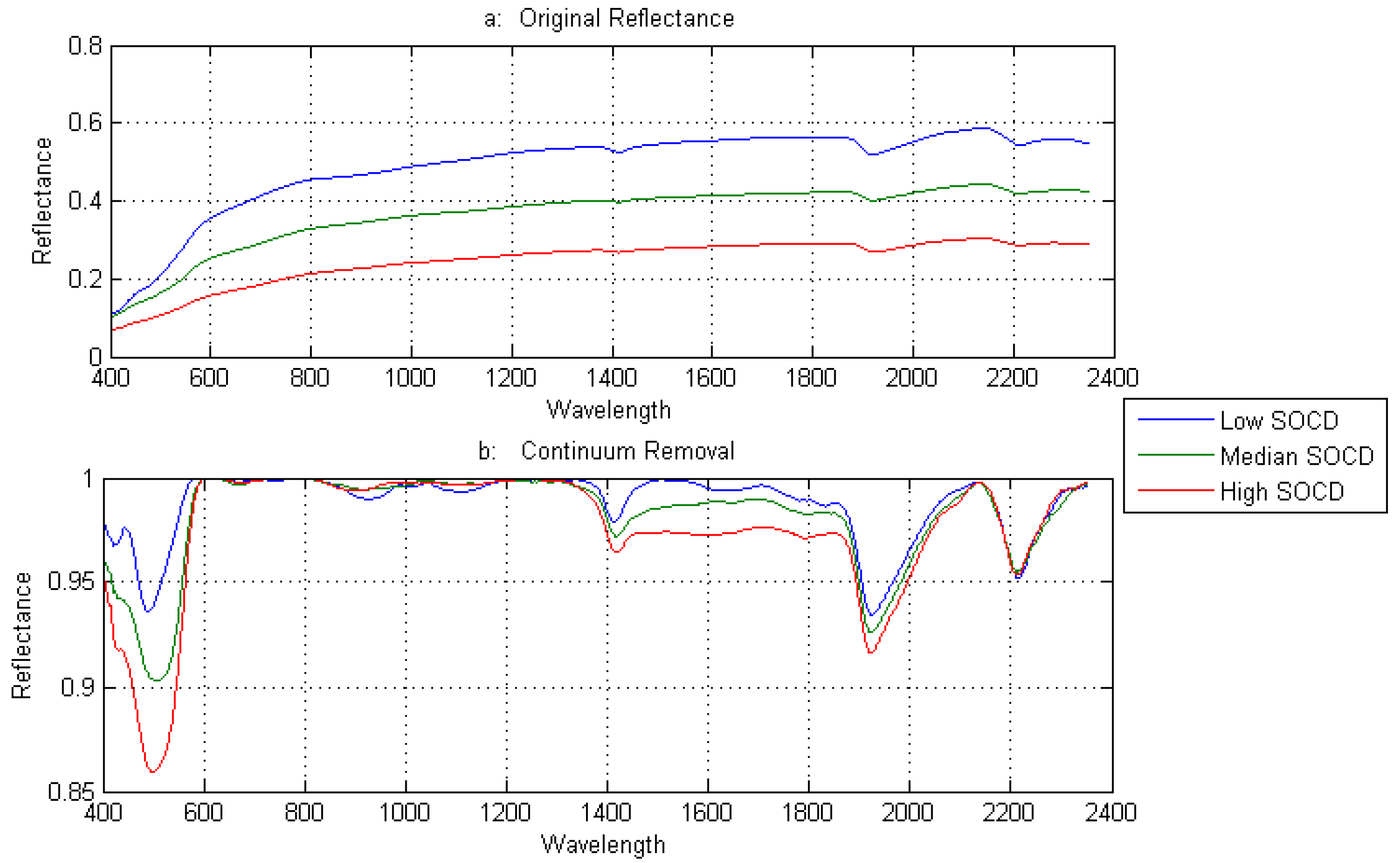
3.2. Pretreatment of the Spectral Features

The original and the transformed spectral reflectance of the soil samples are shown in Figure 2. Three SOCD values were selected as representatives of the SOCD contents (high (10.16 kg·m⁻²), median (5.25 kg·m⁻²), and low (0.33 kg·m⁻²)) to illustrate the relationship between SOCD and spectral reflectance. In Figure 2, the highest SOCD showed the lowest spectral reflectance, whereas the lowest SOCD presented the highest spectral reflectance in the entire wavelength. Soil samples generally exhibited four deep and large absorption features at 400–600, 1455, 1915, and 2210 nm. The first spectral absorption feature in the visible wavelengths (400–600 nm) was due to electronic transitions, such as the Fe oxides of the hematite (Fe₂O₃) and goethite (FeOOH) [39]. The dominant absorption near 1455 nm is related to the first overtone of an O–H stretching vibration of water (H–O–H) or metal–O–H vibration [7]. The feature near 1915 nm was related to the combinations of the vibrational processes of water, where H–O–H bends and OH stretches. The absorption near 2210 nm was due to O–H stretching combination vibrations [39]. The absorption features of the transformed spectra were stronger than those of the original spectra at these wavelengths. The drift of the spectra was removed along the entire wavelength (Figure 2b). This result was the same with those of many other studies. That is, the continuum removal technique pretreatment can highlight the absorption features of the spectral reflectance in different wavelengths and subsequently improve the prediction accuracy of the soil spectral models [48,49].

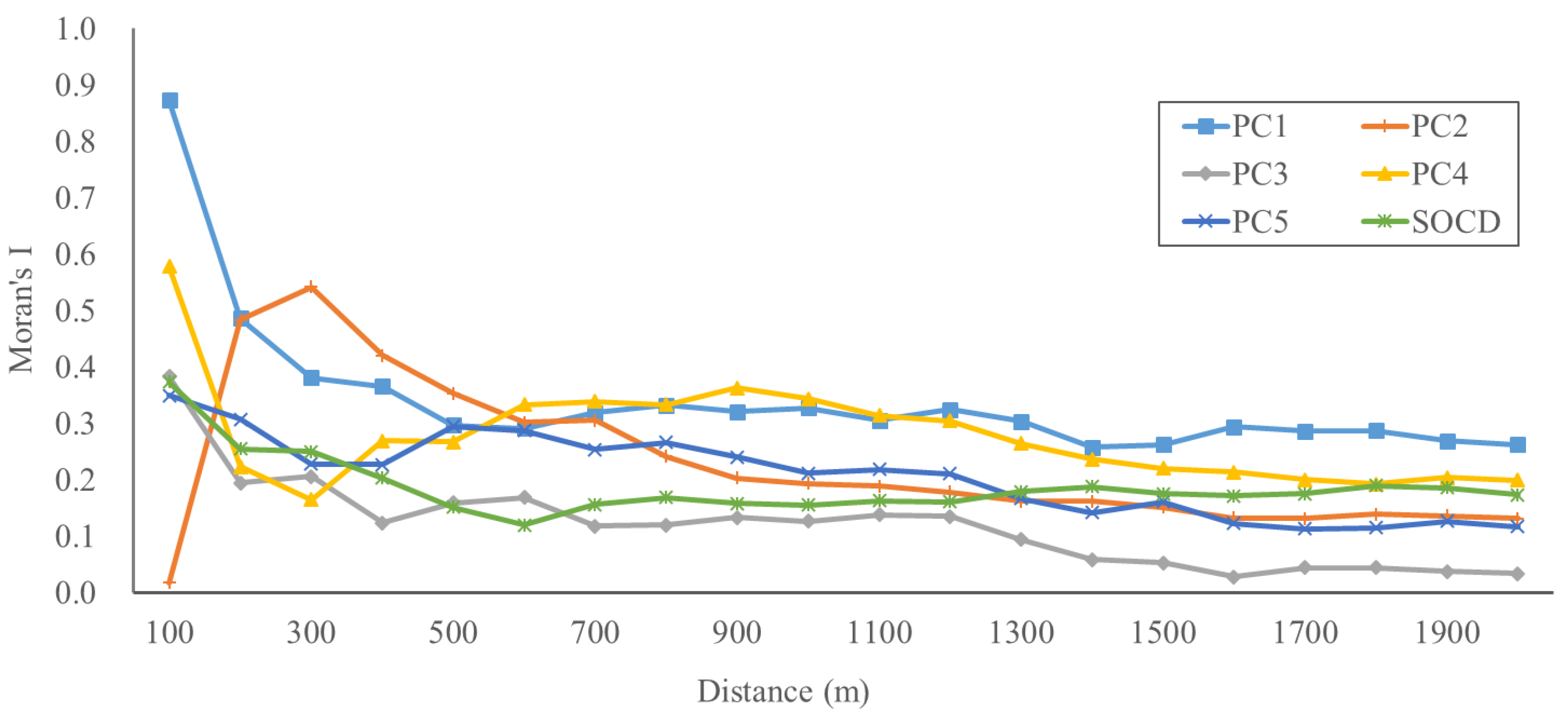
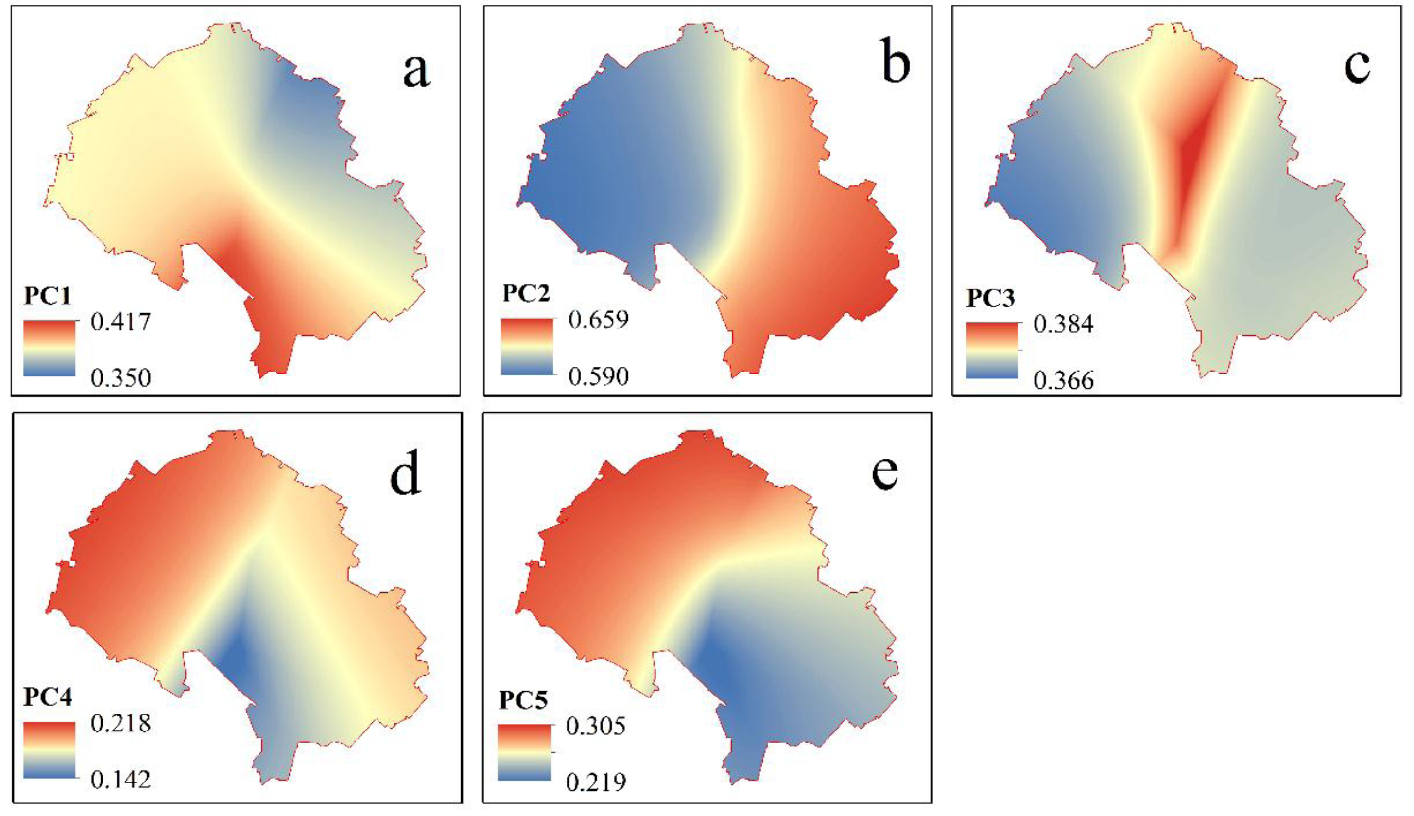
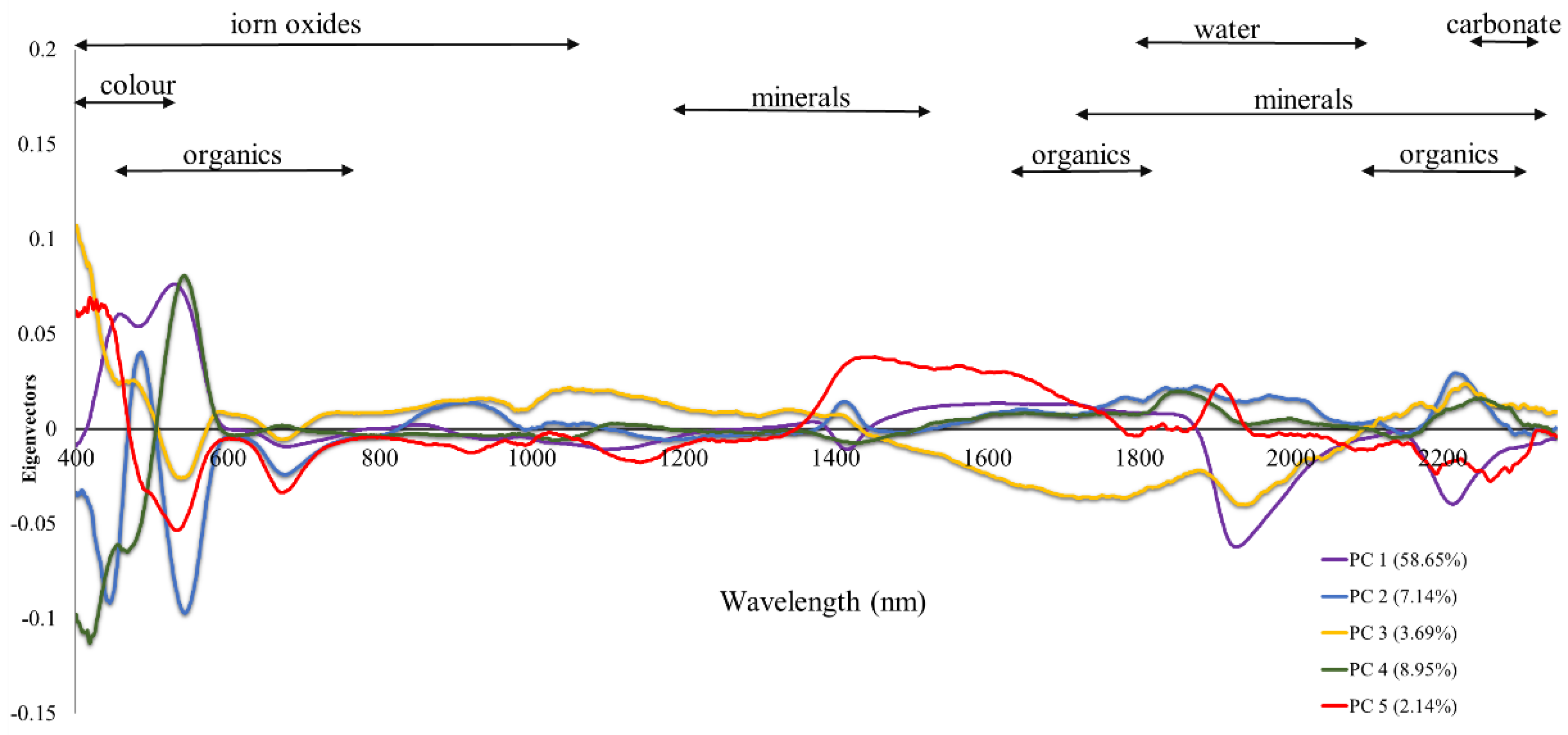
3.3. Spatial Characteristics of the Spectral Reflectance

The first five PCs, which were extracted from the soil spectra by PLSR, were selected as the suitable auxiliary variables based on the leave-one-out cross-validation. A large value of the percent of variance results in a considerable amount of information extracted from the original data [50]. The total percent of variance of the first five PCs was 80.57%. This value implies that the PCs can explain 80.57% of the information to the original spectral reflectance. The basic statistics of the five PCs were used to analyze the global characteristics of the spectral information (

Table 2. The basic statistics of the first five principal components (PCs) of the spectral information which were extracted from the principal least squares regression model.

	The Percentages of Variance	Range	Min	Max	Mean	SD
PC1	58.65%	39.69	−19.32	20.37	0	8.43
PC2	7.14%	17.54	−11.21	6.32	0	2.94
PC3	3.69%	10.18	−5.03	5.14	0	2.12
PC4	8.95%	16.81	−9.8	7.01	0	3.29
PC5	2.14%	9.74	−5.52	4.22	0	1.61

Min: Minimum, Max: Maximum, SD: Standard deviation, PC: principal component.

). The percentages of variance of the five PCs were 58.65%, 7.14%, 3.69%, 8.95%, and 2.14%. PC1 showed the largest percent of variance, and PC5 exhibited the least value. The range of five PCs were 39.69, 17.54, 10.18, 16.81, and 9.74, respectively, and their standard deviation values were 8.43, 2.94, 2.12, 3.29, and 1.61, respectively. This result shows the dispersion degrees of the PCs from their average. PC1 displayed the highest range and standard deviation, which indicate that the data points were distributed over a large range of values. PC5 exhibited the lowest range and standard deviation, which signify that the data points were close to the mean value. When the percent of variance of one PC was larger than those of the other PCs, a large amount of soil information regarding soil physical structure, mineral composition, and organic matter was included in this PC and revealed its significant difference. This finding implies the global non-stationarity of the PCs in the study region.

Moran’s I is a measure of spatial autocorrelation, which is characterized by a correlation in a signal among nearby locations in space [51]. The values of Moran’s I range from −1 to 1. Negative values indicate negative spatial autocorrelation, and positive values indicate positive spatial autocorrelation. A zero value indicates a random spatial pattern [52]. In this paper, Moran’s I index was used to validate the spatial autocorrelation of SOCD and PCs in different sampling distances (Figure 3). In the global trend, the Moran’s I values of SOCD and PCs decreased with increased sampling distance. The highest Moran’s I value of SOCD was 0.37 at 100 m. The value indicates that positive spatial autocorrelation existed in the SOCD. The highest of Moran’s I values of PC1, PC3, PC4, and PC5 were 0.87, 0.38, 0.58, and 0.35, respectively, at 100 m and that of PC2 was 0.54 at 300 m. These results show that a positive spatial autocorrelation also existed in the input variables (SOCD and the spectral reflectance) of the soil spectral models. Therefore, one spatial model relative to the traditional non-spatial model should be constructed. PC1 was the strongest, PC2 and PC4 were the second, and PC3 and PC5 were the least. This order was the same as that of the percentages of variance of the PCs in PLSR. When the percent of variance was large, the obtained soil information was also large. When one PC contained a considerable amount of soil information, the spatial characteristics of the soil samples were easily correlated with the PC. Thus, PC1 showed the strongest spatial autocorrelation for the greatest soil information, whereas PC5 exhibited the weakest spatial autocorrelation for the lowest soil information.

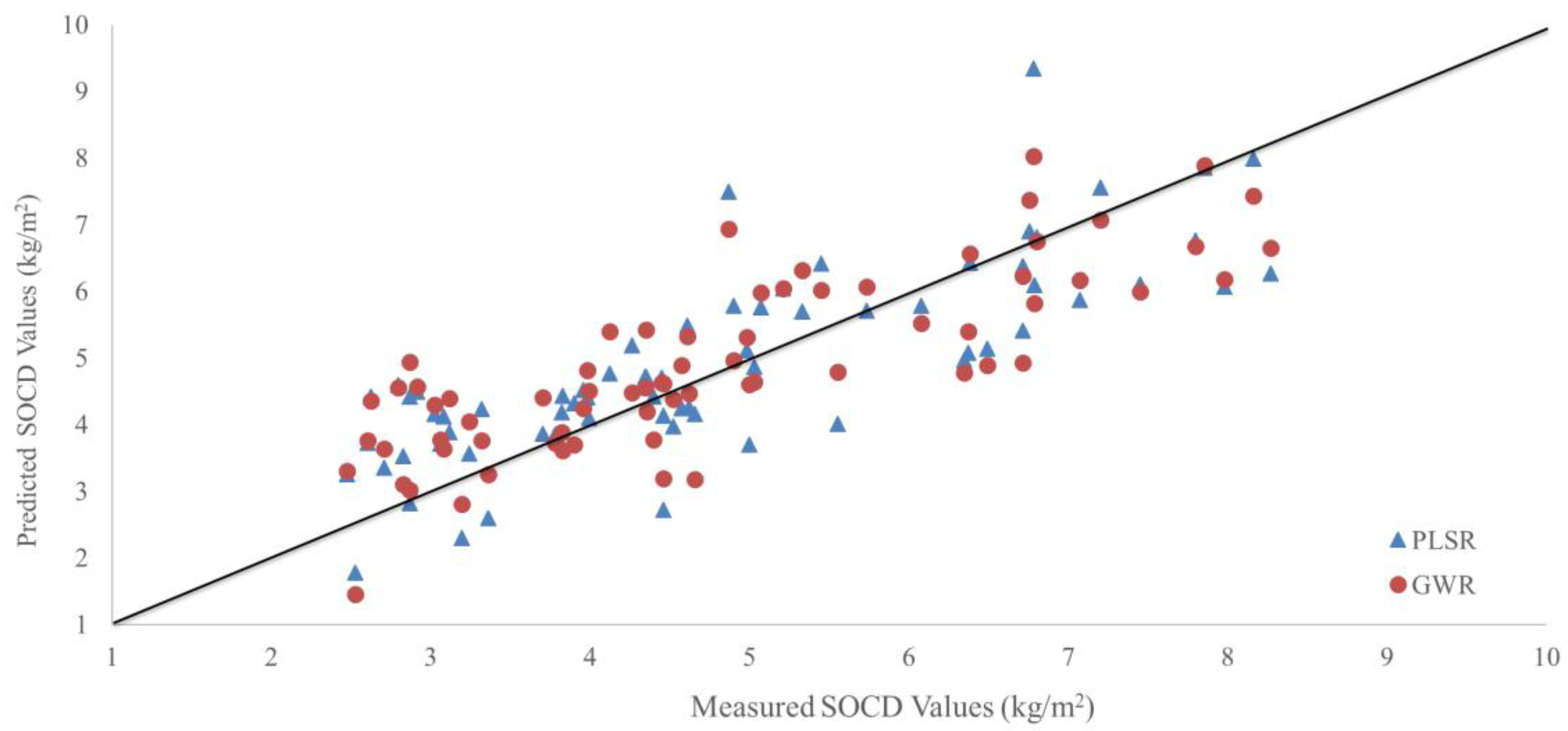
3.4. Prediction of SOCD by PLSR and GWR

In PLSR model, the first five PCs were selected to construct the SOCD prediction model with the aid of the spectral reflectance. These five PCs were also used as the auxiliary variables to construct the GWR model. The basic statistics of the parameters of PLSR and GWR are shown in

Table 3. Summary of global and local coefficients used in soil organic carbon density (SOCD) model by principal least squares regression (PLSR) and geographically weighted regression (GWR) models.

	Global Coefficients (PLSR)				Local Coefficients (GWR)
Variables	Coefficients	SCs	t-Values	p-Values	Range	Min	Max	Mean	Mean of SCs	Std
Intercept	5.368		74.95	0	0.110	5.315	5.425	5.366		0.026
PC1	0.089	0.384	10.469	0	0.010	0.084	0.094	0.089	0.383	0.002
PC2	0.415	0.623	17.003	0	0.042	0.393	0.435	0.413	0.620	0.014
PC3	0.339	0.366	9.99	0	0.015	0.34	0.355	0.345	0.373	0.003
PC4	0.125	0.210	5.724	0	0.037	0.09	0.127	0.112	0.188	0.009
PC5	0.342	0.280	7.665	0	0.093	0.27	0.363	0.323	0.265	0.030

PLSR: partial least squares regression; GWR: geographically weighted regression; SC: standardized coefficient; Min: minimum; Max: maximum; Std: standard deviation; PC: principal component.

. The coefficients of PCs were constant in PLSR, which showed that the influence degree of one PC on SOCD was the same as in the total study region. The coefficients of these five PCs were 0.089, 0.415, 0.339, 0.125, and 0.342. The coefficients of these PCs were positive, which implied the positive correlations between PC and SOCD. Given the different PCs, including different spectral information related to different soil components, the PC coefficients were influenced by the units of different soil components. Thus, the PC coefficients should be standardized to remove the differences of the PC units. The Z-score method was used to standardize the coefficients of PCs, and the standardized coefficient (SC) was used to label the new coefficient. SC can show which of the PCs exerted a remarkable effect on SOCD in soil spectral models. The SCs of these five PCs were 0.384, 0.623, 0.366, 0.210, and 0.280. The descending order of these coefficients was PC2 > PC1 > PC3 > PC5 > PC4. PC2 showed the most significant effects on SOCD, whereas PC4 exerted the least significant effects. The t- and p-values, which showed the significance of PCs in predicting SOCD by PLSR, are presented in Table 3.

GWR is a local spatial model that allows the flexible coefficients of auxiliary variables in different geographical locations. The basic statistics of the coefficients of PCs in the GWR are shown in Table 3. The ranges of the coefficients of the PCs in descending order were PC5 (0.093), PC2 (0.042), PC4 (0.037), PC3 (0.015), and PC1 (0.010). The range of the coefficient of PC5 was wider than those of the other PCs. This range showed the largest uncertainty of the PC5 coefficient in the different geographical locations. The influence degrees of PCs on SOCD were described by the SCs, and the spatial distribution characteristics of SCs are shown in Figure 4. The descending order of the mean values of SCs was PC2 (0.620) > PC1 (0.383) > PC3 (0.373) > PC5 (0.265) > PC4 (0.188) (Table 3). This order was similar to that of PLSR where PC2 exerted the most significant influence, and PC4 presented the least significant effect. Such result was due to the percent of variance and the valuable spectral information of PCs. The percent of variance can influence the total content of the spectral information of PC, but a large percent of variance does not imply a large amount of valuable spectral information. Furthermore, the valuable spectral information can influence the degree of correlation between a PC and SOCD. Thus, the SCs can also show which PCs play important roles in predicting the SOCD. Afterward, the soil components related to the PCs can be further explored.

Soil properties are influenced by the microtopography, soil microorganism, soil water content, and temperature conditions of a local region. These environmental factors vary with geographical location. Hence, the spectral reflectance of different soil samples differs. The relationships between PCs and SOCD also varied with geographical location. GWR, as a local spatial weight model, considers the spatial autocorrelation of SOCD and PCs to construct prediction models. The coefficient maps of PCs showed variable relationships between PCs and SOCD (Figure 4). PLSR, as a global linear regression model, assumes that the influence degrees of PCs on SOCD are the same in the study region. Therefore, the GWR parameters can provide a considerable amount of information to explore the relationships between spectral reflectance and SOCD in different geographical locations.

3.5. Model Validation and Evaluation

Detailed information on the evaluation indexes is presented in

Table 4. The basic statistics of different evaluation indices by principal least squares regression (PLSR) and geographically-weighted regression (GWR) models.

Model	RMSEC (kg·m−2)	RMSEP (kg·m−2)	R2C	R2P	RPD
PLSR	0.892	0.985	0.791	0.631	1.646
GWR	0.875	0.950	0.800	0.654	1.702

RMSE: the root mean square error; RPD: the ratio of percentage deviation; PLSR: partial least squares regression; GWR: geographically weighted regression.

. According to the classification of Chang, et al. [53], the RPD values of PLSR and GWR were 1.646 and 1.702, respectively, which were located between 1.4 and 2.0. This result showed that PLSR and GWR exhibited good prediction accuracy in predicting SOCD by VNIRS. Thus, the potential ability of VNIRS in predicting SOCD was high, and PLSR and GWR can guarantee a feasible and reliable prediction accuracy. The predicted values of SOCD by GWR and PLSR were also drawn in the scatter plot (Figure 5). Most of the predicted values were distributed around the 1:1 line, thereby showing a high prediction accuracy of PLSR and GWR in predicting SOCD by VNIRS. Moreover, the evaluation indexes shown in Table 4 revealed that GWR presented a superior modeling and predicting ability to that of PLSR because GWR possessed smaller RMSE_C and RMSE_P and higher R²_C, R²_P, and RPD than those of PLSR. This result was due to the finding that SOCD and PCs exhibited a spatial autocorrelation. In addition, the GWR considered their spatial autocorrelation in constructing the prediction models. In conclusion, VNIRS showed a significant potential in predicting SOCD, and the spatial autocorrelation of VNIRS played an important role in the soil spectral models. GWR exhibited a better modeling performance and prediction accuracy than those of PLSR.

4. Discussion

4.1. Spatial Autocorrelation and Nonstationarity of PCs

The relationships between VNIRS, PCs, and SOCD played important roles in guaranteeing the prediction accuracy and the stability of the soil spectral models. Eigenvectors can be used to quantify the relationships between VNIRS and PCs (Figure 6). Furthermore, the regression coefficients can be used to quantify the relationships between PCs and SOCD (Table 3). Spatial autocorrelation exists in soil properties [54], and the spectral reflectance is the response of the physical and chemical properties of soil. Thus, spatial autocorrelation also existed in the VNIRS and PCs. Moran’s I can be used to show the degree of the spatial autocorrelation of the PCs in different sampling distances (Figure 3). The spatial autocorrelation is a characteristic attribute of thematic maps. That is, the polygons on a map represent zones where the internal variation is small relative to that of the variation in the map as a whole. Furthermore, the random spatial autocorrelation would exhibit no apparent spatial pattern and thus appear as white noise [55]. Additionally, the strong spatial autocorrelation also implies the abundant spatial and spectral information when the Moran’s I is close to 1. Meanwhile, the random spatial autocorrelation indicates the weak spatial and spectral information when the Moran’s I is close to 0 [56]. In the present study, the descending order of the regression coefficients of PCs was PC2, PC1, PC3, PC5, and PC4. This order was similar to that of Moran’s I values when the sampling distance was 300 m, which was the average distance between different soil samples. PC2 contained the most abundant spectral and spatial information. Hence, PC2 exhibited the strongest relationships with the SOCD. Many white noises existed in PC4 and suggest the PC’s weak role in predicting the SOCD. Therefore, the spatial autocorrelation and the regression coefficients can show the spatial and spectral information of PCs, as well as the influence degrees of the PCs to the SOCD. The average distance of the soil samples is one important parameter that connects the relationships between Moran’s I values and the regression coefficients.

The absorption and reflection spectral features of VNIRS were influenced by different physical and chemical characteristics of soil. These attributes include the color, mineral content, soil moisture, and soil texture. The spectral reflectance can show the spectral characteristics of the soil in different wavelengths, and the continuum removal method can strengthen the absorption features relative to the original spectra (Figure 2). The eigenvectors can show the relationships between the spectral reflectance and the PCs in different wavelengths (Figure 6). Comparison of the differences between the spectral reflectance after transformation and the eigenvectors in different wavelengths show that large wave ranges of the eigenvectors appeared at the soil absorption features. These ranges included 400–600, 1400, 1800–2000, and 2200 nm. These absorption features displayed strong relationships with organic matters and minerals. Consequently, the first five PCs can reflect the main information of the spectra, and they exhibited strong relationships with the organic matters and minerals in soil. The different chemical and physical materials of soil exerted different influence degrees to SOCD at different geographical locations. The SCs of PCs can also show these relationships (Figure 4). Thus, the GWR model can offer further information to understand and explore the relationships between PCs and SOCD. The spatial autocorrelation and nonstationarity of PCs should also be considered when constructing soil spectral models.

4.2. Advantages of GWR

The SOCD levels are often associated with environmental factors (e.g., climate, parent material, biology, terrain, and time) and human activities (e.g., land use types and tillage management) [57]. In neighboring soil samples, soil types share similar environmental factors and human activities. This sharing results in the spatial dependence of soil properties. Additionally, the differences in these auxiliary factors influence the spatial heterogeneity of soil properties. Moran’s I values showed that spatial autocorrelation existed in SOCD and its PCs. The values further revealed the order of the spatial autocorrelation degrees of PCs. Thus, the spatial autocorrelation of the SOCD and PCs should be considered when soil samples are gathered in one small-scale study region. GWR, as a local spatial regression model, considers the spatial autocorrelation of explanatory variables (spectra or environmental factors) and explained variables (soil properties). This method reflects the variation of the spatial weights of PCs to the SOCD in different geographical locations [22]. The predictive ability of GWR outperforms that of traditional regression models because these models contain no spatial information on the input variables. Moreover, the influence degrees of explanatory variables on the explained variables are constant in the study region. Kumar, et al. [58] used 1424 georeferenced soil profiles and a total of 20 variables, including terrain attributes, climate data, bedrock geology, and land use data to map the SOCD by GWR and MLR. Song, et al. [28] used GWR and MLR to predict the SOC content in the Heihe River Basin in China by environmental covariates. All of these studies showed an excellent estimation and explanation of GWR relative to MLR and the spatial non-stationarity of environmental covariates in predicting SOCD. Although the auxiliary variables were environmental factors, the spatial autocorrelation of SOCD and the spatial nonstationarity of explanatory variables played important roles in constructing soil models.

VNIRS directly responds to the chemical and physical structures of soil. Valuable spectral information was extracted from the original spectra to compose the new auxiliary variables (PCs). The existence of spatial dependence in soil was proven. Therefore, spatial dependence also played an important role in soil spectra and PCs. VNIRS technique is a rapid, nondestructive, and cost-effective method to predict soil properties. However, most of these methods do not consider the spatial dependence of soil properties and VNIRS in the modeling processes [11,38]. Many scholars also realized the importance of spatial characteristics of soil spectra in constructing soil spectral models [16,21,59]. The linear mixed effect model was used by Conforti et al. [21]. Meanwhile, the ordinary kriging was used by Ge et al. [16,21] to weaken the influence of the spatial autocorrelation of spectral reflectance on the prediction accuracy of soil spectral models. Guo et al. [22] also showed that GWR can consider the spatial autocorrelation of soil properties and spectral reflectance to improve its prediction accuracy over that of PLSR. These investigations offered important theoretical basis to explore the application of spatial autocorrelation in predicting one complicated composition (SOCD). The present study showed that the prediction accuracy of GWR in predicting SOCD by spectral reflectance was higher than that of PLSR. Furthermore, the spatial nonstationarity of PCs in predicting SOCD was shown by the coefficient map of GWR. GWR was advantageous because it considered the spatial dependence of input variables in constructing soil models and explained the ability of the spatial variable relationships between PCs and SOCD in different geographical locations.

Although GWR exhibited advantages relative to PLSR in constructing soil spectral models, many other uncertain factors existed and influenced the prediction results. These factors included the scale of the study area, the density of the soil samples, and the preprocessing methods of the spectra. The spatial autocorrelation of the spectral reflectance was calculated by the discrete soil samples. The soil samples were used to measure the spectra after a series of preprocessing methods. Consequently, considerable amount of time and labor were needed to prepare the soil samples. Additionally, the discrete spectral data cannot reflect the total spatial characteristics of the soil in the study region. Therefore, numerous technical details and factors should be considered in future studies when using GWR to predict soil properties by soil spectra. The continuous hyperspectral images can also be used to construct the spatial models.

5. Conclusions

This study explored the need for the spatial dependence of SOCD and soil spectra in predicting SOCD. This need was investigated by the local spatial regression model (GWR) and the traditional linear regression model (PLSR). Spatial dependence and spatial heterogeneity existed in both the soil attributes and spectral reflectance. Thus, spatial information played an important role in guaranteeing the efficiency and accuracy of the soil spectral models. In the prediction models, the evaluation indexes showed that GWR exhibited a better prediction accuracy (RPD = 1.702) than that of PLSR (RPD = 1.646) for SOCD. This result was mainly attributed to that the spatial autocorrelation of PCs. This autocorrelation can offer valuable auxiliary information to strengthen the relationships between neighboring soil samples. Moreover, Moran’s I index verified that spatial autocorrelation existed in the SOCD and its PCs. Such correlation also displayed strong positive relationships with the regression coefficients of the prediction models at the average sampling distance (300 m). The PC eigenvectors were influenced by the absorption features of the spectral reflectance due to the soil’s different physical and chemical attributes. The coefficient maps of GWR showed that the influence degrees of PCs on the SOCD varied with geographical location. This study contributed in further understanding the underlying mechanism why soil spectra exhibit spatial dependence and how spatial models should be applied in predicting soil properties in future research.

References

1. Pataki, D.; Alig, R.; Fung, A.; Golubiewski, N.; Kennedy, C.; McPherson, E.; Nowak, D.; Pouyat, R.; Romero Lankao, P. Urban ecosystems and the North American carbon cycle. Glob. Chang. Biol. 2006, 12, 2092–2102. [Google Scholar] [CrossRef]
2. Hoffmann, U.; Hoffmann, T.; Jurasinski, G.; Glatzel, S.; Kuhn, N. Assessing the spatial variability of soil organic carbon stocks in an alpine setting (Grindelwald, Swiss Alps). Geoderma 2014, 232, 270–283. [Google Scholar] [CrossRef]
3. Vasques, G.; Grunwald, S.; Sickman, J. Comparison of multivariate methods for inferential modeling of soil carbon using visible/near-infrared spectra. Geoderma 2008, 146, 14–25. [Google Scholar] [CrossRef]
4. Eswaran, H.; van Den Berg, E.; Reich, P. Organic carbon in soils of the world. Soil Sci. Soc. Am. J. 1993, 57, 192–194. [Google Scholar] [CrossRef]
5. Wang, S.-q.; Zhou, C.-h.; Li, K.-r.; Zhu, S.-l.; Huang, F.-h. Estimation of soil organic carbon reservoir in China. J. Geogr. Sci. 2001, 11, 3–13. [Google Scholar]
6. Viscarra Rossel, R.A.; Walvoort, D.J.J.; McBratney, A.B.; Janik, L.J.; Skjemstad, J.O. Visible, near infrared, mid infrared or combined diffuse reflectance spectroscopy for simultaneous assessment of various soil properties. Geoderma 2006, 131, 59–75. [Google Scholar] [CrossRef]
7. Stenberg, B.; Rossel, R.A.V.; Mouazen, A.M.; Wetterlind, J. Visible and near infrared spectroscopy in soil science. In Advances in Agronomy, Vol 107; Sparks, D.L., Ed.; Elsevier: Boston, MA, USA, 2010; pp. 163–215. [Google Scholar]
8. Viscarra Rossel, R.A.; Hicks, W.S. Soil organic carbon and its fractions estimated by visible-near infrared transfer functions. Eur. J. Soil Sci. 2015, 66, 438–450. [Google Scholar] [CrossRef]
9. Gomez, C.; Rossel, R.A.V.; McBratney, A.B. Soil organic carbon prediction by hyperspectral remote sensing and field VIS-NIR spectroscopy: An Australian case study. Geoderma 2008, 146, 403–411. [Google Scholar] [CrossRef]
10. Sreenivas, K.; Sujatha, G.; Sudhir, K.; Kiran, D.V.; Fyzee, M.A.; Ravisankar, T.; Dadhwal, V.K. Spatial assessment of soil organic carbon density through random forests based imputation. J. Indian Soc. Remote Sens. 2014, 42, 577–587. [Google Scholar] [CrossRef]
11. Bellon-Maurel, V.; McBratney, A. Near-infrared (NIR) and mid-infrared (MIR) spectroscopic techniques for assessing the amount of carbon stock in soils—Critical review and research perspectives. Soil Biol. Biochem. 2011, 43, 1398–1410. [Google Scholar] [CrossRef]
12. Le Guillou, F.; Wetterlind, W.; Rossel, R.V.; Hicks, W.; Grundy, M.; Tuomi, S. How does grinding affect the mid-infrared spectra of soil and their multivariate calibrations to texture and organic carbon? Soil Res. 2015, 53, 913–921. [Google Scholar] [CrossRef]
13. Stenberg, B. Effects of soil sample pretreatments and standardised rewetting as interacted with sand classes on VIS-NIR predictions of clay and soil organic carbon. Geoderma 2010, 158, 15–22. [Google Scholar] [CrossRef]
14. Shi, T.; Chen, Y.; Liu, Y.; Wu, G. Visible and near-infrared reflectance spectroscopy—An alternative for monitoring soil contamination by heavy metals. J. Hazard. Mater. 2014, 265, 166–176. [Google Scholar] [CrossRef] [PubMed]
15. Araujo, S.R.; Wetterlind, J.; Dematte, J.A.M.; Stenberg, B. Improving the prediction performance of a large tropical VIS-NIR spectroscopic soil library from brazil by clustering into smaller subsets or use of data mining calibration techniques. Eur. J. Soil Sci. 2014, 65, 718–729. [Google Scholar] [CrossRef]
16. Ge, Y.; Thomasson, J.A.; Morgan, C.L.; Searcy, S.W. VNIR diffuse reflectance spectroscopy for agricultural soil property determination based on regression-kriging. Trans. ASABE 2007, 50, 1081–1092. [Google Scholar] [CrossRef]
17. Wang, J.; Yang, R.; Bai, Z. Spatial variability and sampling optimization of soil organic carbon and total nitrogen for minesoils of the loess plateau using geostatistics. Ecol. Eng. 2015, 82, 159–164. [Google Scholar] [CrossRef]
18. Javed, I.; Thomasson John, A.; Jenkins Johnie, N.; Owens Phillip, R.; Whisler Frank, D. Spatial variability analysis of soil physical properties of alluvial soils. Soil Sci. Soc. Am. J. 2005, 69, 1338–1350. [Google Scholar]
19. Viscarra Rossel, R.A.V.; Rizzo, R.; Demattê, J.A.M.; Behrens, T. Spatial modeling of a soil fertility index using visible-near-infrared spectra and terrain attributes. Soil Sci. Soc. Am. J. 2010, 74, 1293–1300. [Google Scholar] [CrossRef]
20. Guerrero, C.; Wetterlind, J.; Stenberg, B.; Mouazen, A.M.; Gabarrón-Galeote, M.A.; Ruiz-Sinoga, J.D.; Zornoza, R.; Rossel, R.A.V. Do we really need large spectral libraries for local scale soc assessment with nir spectroscopy? Soil Tillage Res. 2016, 155, 501–509. [Google Scholar] [CrossRef]
21. Conforti, M.; Castrignano, A.; Robustelli, G.; Scarciglia, F.; Stelluti, M.; Buttafuoco, G. Laboratory-based VIS-NIR spectroscopy and partial least square regression with spatially correlated errors for predicting spatial variation of soil organic matter content. Catena 2015, 124, 60–67. [Google Scholar] [CrossRef]
22. Guo, L.; Zhao, C.; Zhang, H.; Chen, Y.; Linderman, M.; Zhang, Q.; Liu, Y. Comparisons of spatial and non-spatial models for predicting soil carbon content based on visible and near-infrared spectral technology. Geoderma 2017, 285, 280–292. [Google Scholar] [CrossRef]
23. Gasch, C.K.; Huzurbazar, S.V.; Stahl, P.D. Small-scale spatial heterogeneity of soil properties in undisturbed and reclaimed sagebrush steppe. Soil Tillage Res. 2015, 153, 42–47. [Google Scholar] [CrossRef]
24. Brunsdon, C.; Fotheringham, S.; Charlton, M. Geographically weighted regression. J. R. Stat. Soc. Ser. D 1998, 47, 431–443. [Google Scholar] [CrossRef]
25. Fotheringham, A.S.; Brunsdon, C.; Charlton, M. Geographically Weighted Regression: The Analysis of Spatially Varying Relationships; Wiley: Hoboken, NJ, USA, 2003. [Google Scholar]
26. Kumar, S.; Lal, R.; Liu, D. A geographically weighted regression kriging approach for mapping soil organic carbon stock. Geoderma 2012, 189, 627–634. [Google Scholar] [CrossRef]
27. Sun, W.; Zhu, Y.Q.; Huang, S.L.; Guo, C.X. Mapping the mean annual precipitation of China using local interpolation techniques. Theor. Appl. Climatol. 2015, 119, 171–180. [Google Scholar] [CrossRef]
28. Song, X.-D.; Brus, D.J.; Liu, F.; Li, D.-C.; Zhao, Y.-G.; Yang, J.-L.; Zhang, G.-L. Mapping soil organic carbon content by geographically weighted regression: A case study in the Heihe river basin, China. Geoderma 2016, 261, 11–22. [Google Scholar] [CrossRef]
29. Lado, L.R.; Hengl, T.; Reuter, H.I. Heavy metals in european soils: A geostatistical analysis of the foregs geochemical database. Geoderma 2008, 148, 189–199. [Google Scholar] [CrossRef]
30. Gong, Z. Chinese Soil Taxonomy; Science Press: Beijing, China, 2001. [Google Scholar]
31. Food and Agriculture Organization of the United Nations. World Reference Base for Soil Resources; Food and Agriculture Organization of the United Nations: Rome, Italy, 1998. [Google Scholar]
32. Le zhi, W.U.; Cai, Z.C. The relationship between the spatial scale and the variation of soil organic matter in China. Adv. Earth Sci. 2006, 21, 965–972. [Google Scholar]
33. Nelson, D.W.; Sommers, L.E.; Sparks, D.L.; Page, A.L.; Helmke, P.A.; Loeppert, R.H.; Soltanpour, P.N.; Tabatabai, M.A.; Johnston, C.T.; Sumner, M.E. Total carbon, organic carbon, and organic matter. In Methods of Soil Analysis Part—Chemical Methods; American Society of Agronomy, Soil Science Society of America: Madison, WI, USA, 1982; pp. 961–1010. [Google Scholar]
34. Ivezić, V.; Kraljević, D.; Lončarić, Z.; Engler, M.; Kerovec, D.; Zebec, V.; Jović, J. Organic Matter Determined by Loss on Ignition and Potassium Dichromate Method. In Proceedings of the 51st Croatian and 11th International Symposium on Agriculture, Opatija, Croatia, 15–18 February 2016. [Google Scholar]
35. McKenzie, N.; Jacquier, D.; Ashton, L.; Cresswell, H. Estimation of soil properties using the atlas of Australian soils. CSIRO Land Water Tech. Rep. 2000, 11, 1–12. [Google Scholar]
36. Calhoun, F.G.; Smeck, N.E.; Slater, B.L.; Bigham, J.M.; Hall, G.F. Predicting bulk density of ohio soils from morphology, genetic principles, and laboratory characterization data. Soil Sci. Soc. Am. J. 2001, 65, 811–819. [Google Scholar] [CrossRef]
37. Thompson, J.A.; Kolka, R.K. Soil carbon storage estimation in a forested watershed using quantitative soil-landscape modeling. Soil Sci. Soc. Am. J. 2005, 69, 1086–1093. [Google Scholar] [CrossRef]
38. Shi, T.Z.; Chen, Y.Y.; Liu, H.Z.; Wang, J.J.; Wu, G.F. Soil organic carbon content estimation with laboratory-based visible-near-infrared reflectance spectroscopy: Feature selection. Appl. Spectrosc. 2014, 68, 831–837. [Google Scholar] [CrossRef] [PubMed]
39. Viscarra Rossel, R.A.V.; Behrens, T. Using data mining to model and interpret soil diffuse reflectance spectra. Geoderma 2010, 158, 46–54. [Google Scholar] [CrossRef]
40. Geladi, P.; Kowalski, B.R. Partial least-squares regression: A tutorial. Anal. Chim. Acta 1986, 185, 1–17. [Google Scholar] [CrossRef]
41. Harald, M.; Paul, G. Multivariate calibration. Technometrics 1991, 1158, 61. [Google Scholar]
42. Charlton, M.; Fotheringham, S.; Brunsdon, C. Geographically weighted regression. In White Paper: National Centre for Geocomputation; National University of Ireland Maynooth: Maynooth, Ireland, 2009. [Google Scholar]
43. Fotheringham, A.S.; Brunsdon, C.; Charlton, M. Geographically Weighted Regression; Wiley: New York, NY, USA, 2002. [Google Scholar]
44. Hurvich, C.M.; Simonoff, J.S.; Tsai, C.L. Smoothing parameter selection in nonparametric regression using an improved akaike information criterion. J. R. Stat. Soc. Ser. B Stat. Methodol. 1998, 60, 271–293. [Google Scholar] [CrossRef]
45. Gogé, F.; Gomez, C.; Jolivet, C.; Joffre, R. Which strategy is best to predict soil properties of a local site from a national VIS–NIR database? Geoderma 2014, 213, 1–9. [Google Scholar] [CrossRef]
46. Galvão, R.K.H.; Araujo, M.C.U.; José, G.E.; Pontes, M.J.C.; Silva, E.C.; Saldanha, T.C.B. A method for calibration and validation subset partitioning. Talanta 2005, 67, 736–740. [Google Scholar] [CrossRef] [PubMed]
47. Buchmann, N. Biotic and abiotic factors controlling soil respiration rates in Picea abies stands. Soil Biol. Biochem. 2000, 32, 1625–1635. [Google Scholar] [CrossRef]
48. Viscarra Rossel, R.; Cattle, S.; Ortega, A.; Fouad, Y. In situ measurements of soil colour, mineral composition and clay content by VIS–NIR spectroscopy. Geoderma 2009, 150, 253–266. [Google Scholar] [CrossRef]
49. Peng, X.; Shi, T.; Song, A.; Chen, Y.; Gao, W. Estimating soil organic carbon using VIS/NIR spectroscopy with SVMR and SPA methods. Remote Sens. 2014, 6, 2699–2717. [Google Scholar] [CrossRef]
50. Abdi, H.; Williams, L.J. Principal component analysis. Wiley Interdiscip. Rev. Comput. Stat. 2010, 2, 433–459. [Google Scholar] [CrossRef]
51. Bartlett, M.S. Notes on continuous stochastic phenomena. Biometrika 1950, 37, 17. [Google Scholar]
52. Cliff, A.D.; Ord, J.K. Spatial Processes: Models & Applications; Pion: London, UK, 1981. [Google Scholar]
53. Chang, C.-W.; Laird, D.A.; Mausbach, M.J.; Hurburgh, C.R. Near-infrared reflectance spectroscopy–principal components regression analyses of soil properties. Soil Sci. Soc. Am. J. 2001, 65, 480–490. [Google Scholar] [CrossRef]
54. Yoon, T.K.; Noh, N.J.; Han, S.; Kwak, H.; Lee, W.K.; Son, Y. Small-scale spatial variability of soil properties in a Korean swamp. Landsc. Ecol. Eng. 2015, 11, 303–312. [Google Scholar] [CrossRef]
55. Anselin, L. Local indicators of spatial association—Lisa. Geogr. Anal. 1995, 27, 93–115. [Google Scholar] [CrossRef]
56. Warner, T.A.; Shank, M.C. Spatial autocorrelation analysis of hyperspectral imagery for feature selection. Remote Sens. Environ. 1997, 60, 58–70. [Google Scholar] [CrossRef]
57. Liu, Y.; Guo, L.; Jiang, Q.; Zhang, H.; Chen, Y. Comparing geospatial techniques to predict SOC stocks. Soil Tillage Res. 2015, 148, 46–58. [Google Scholar] [CrossRef]
58. Kumar, S.; Lal, R.; Liu, D.S.; Rafiq, R. Estimating the spatial distribution of organic carbon density for the soils of Ohio, USA. J. Geogr. Sci. 2013, 23, 280–296. [Google Scholar] [CrossRef]
59. Bilgili, A.V.; Akbas, F.; van Es, H.M. Combined use of hyperspectral VNIR reflectance spectroscopy and kriging to predict soil variables spatially. Precis. Agric. 2011, 12, 395–420. [Google Scholar] [CrossRef]
Figure 1. The spatial distribution of the soil samples in the study area.
Ijgi 06 00308 g001
Figure 2. The original (a) and continuum removal responses (b) of the spectral reflectance of the representative soil organic carbon density contents. SOCD: soil organic carbon density, High SOCD: 10.16 kg·m−2, median SOCD: 5.25 kg·m−2 and low SOCD: 0.33 kg·m−2
Ijgi 06 00308 g002
Figure 3. Moran’s I index of soil organic carbon density (SOCD) and principal components (PCs) in different distances.
Ijgi 06 00308 g003
Figure 4. The spatial distribution of the standardized coefficients of principal components (PCs) in geographically-weighted regression model.
Ijgi 06 00308 g004
Figure 5. The scatter plot of the measured and predicted soil organic carbon density (SOCD) values of the validation dataset by principal least squares regression (PLSR) and geographically-weighted regression (GWR) models.
Ijgi 06 00308 g005
Figure 6. The relationships between the spectral reflectance and principal components (PCs) in different wavelengths.
Ijgi 06 00308 g006