Improving Destination Choice Modeling Using Location-Based Big Data


1
Institute for Transport Planning and Systems, ETH Zürich, CH-8093 Zurich, Switzerland
2
Department of Civil, Geo and Environmental Engineering, Technical University of Munich, Modeling Spatial Mobility, 80333 Munich, Germany
*
Author to whom correspondence should be addressed.
ISPRS Int. J. Geo-Inf. 2017, 6(9), 291; https://doi.org/10.3390/ijgi6090291
Submission received: 30 July 2017
/
Revised: 15 September 2017
/
Accepted: 18 September 2017
/
Published: 20 September 2017
(This article belongs to the Special Issue Geospatial Big Data and Transport)
Abstract
:Citizens are increasingly sharing their location and movements through “check-ins” on location based social networks (LBSNs). These services are collecting unprecedented amounts of big data that can be used to study how we travel and interact with our environment. This paper presents the development of a long distance destination choice model for Ontario, Canada, using data from Foursquare to model destination attractiveness. A methodology to collect and process historical check-in counts has been developed, allowing the utility of each destination to be calculated based on the intensity of different activities performed at the destination. Destinations such as national parks and ski areas are very strong attractors of leisure trips, yet do not employ many people and have few residents. Trip counts to such destinations are therefore poorly predicted by models based on population and employment. Traditionally, this has been remedied by extensive manual data collection. The integration of Foursquare data offers an alternative approach to this problem. The Foursquare based destination choice model was evaluated against a traditional model estimated only with population and employment. The results demonstrate that data from LBSNs can be used to improve destination choice models, particularly for leisure travel.
1. Introduction
Destination Choice modeling using multinomial logit models allows for more sophisticated models than the aggregate approaches that have persisted in the field since the 1950s [1]. Despite the opportunities for more advanced representations of destination utility, models still rely mainly on socio-economic indicators such as the population and employment of the destination zone. However, a traveler’s destination choice is not necessarily made based on how many people live and work there. An example demonstrates where such traditional metrics fall short; national parks have no population and little employment but are large attractors of leisure trips. Ski areas are another example of this effect.
Although it is desirable to better represent the zonal utility, destination choice modeling is often characterized by a large set of alternatives [2]. As such, the acquisition of detailed data for each alternative is not a feasible proposition during the development of many transport models. Simma et al. [3] explored such variables in detail for long distance leisure travel in Switzerland, reporting that the data collection work was indeed particularly onerous. This paper presents an alternative approach, using aggregated data from the location based social network (LBSN) Foursquare to represent destination attractiveness in the utility function of a multinomial logit model.
Big data, such as those collected by Foursquare or Twitter, are a “topic du jour” in transport modeling. Rashidi et al. [4] presented the first comprehensive literature review exploring the opportunities and challenges inherit to working with such data, with a special focus on travel demand modeling. They examined the recent applications of social media data to both aggregate and disaggregate models, activity behavior, traffic behavior, incidents and natural disasters. Most previous works use geotagged messages, called “tweets”, from the social media platform Twitter in their analysis. In particular, they emphasize the opportunity to use websites, such as Yelp or Foursquare, to identify trip purposes from the venue classifications of visited places.
Foursquare provides a platform for users to “check-in” to a point of interest (POI), known as a “venue” and provide tips, ratings and reviews. With 50 million monthly active users and over 7.8 billion check-ins to date [5], Foursquare is the largest LBSN. This enormous amount of data can be used in a multitude of ways to explore mobility patterns. In recent relevant research using Foursquare, Lindqvist et al. [6] looked at how and why people use location sharing services such as Foursquare and discussed how users manage their privacy when using such services. Cheng et al. [7] collected 22 million check-ins across 220,000 users to quantitatively assess human mobility patterns. A total of 53% of their check-ins came from Foursquare, highlighting the dominance of Foursquare in the LBSN space. More recently, data-driven approaches to transport modeling and analysis have been developed using Foursquare data. S.A. et al. [8] combined cell phone and Foursquare data to calculate origin–destination (OD) demand matrices. They found that the results generally matched the observed OD travel, though some differences in trip volumes and patterns were evident. Noulas et al. [9] used Foursquare data in a gravity model based on Stouffer’s theory of intervening opportunities [10]. Using a probabalistic modeling approach, Hasan and Ukkusuri [11] extracted the true transition and activity distributions from incomplete trajectory information using Foursquare check-ins in New York City. Their approach reconstructs timing and location sequences from selective user reporting of check-ins. It has wide applications to other sources of geolocated data, which are affected by similar issues of missing information.
Comprehensive travel surveys such as the Transport Survey of Residents of Canada (TSRC) often have a sample size of around only 50,000 records per year. In contrast, big data sources can record the movements of millions of individuals at unprecedented spatial and temporal accuracy [12]. It is important to note that the high temporal and spatial resolution of geolocated big data comes with its own trade-offs. Often social demographic attributes are not available, making it extremely difficult to correctly weigh the sample. Furthermore, publicly available data for research can be limited or highly aggregated and the collection and sampling methodologies are normally not available for validation [13].
Clearly, there is a need to discover ways of combining both “traditional” (travel surveys and census data) and “new” (big) data sources to harness the best attributes of both. In the field of transport modeling, Chaniotakis et al. [14] empirically investigated the potential for social media to augment travel survey data in Thessaloniki, Greece. They performed both temporal and spatial analyses, comparing the level of activity in destination zones between a traditional travel survey and three social media, namely, Foursquare, Facebook and Twitter. Their findings conclude that while social media cannot be used to directly extract demand models, it can be used as an additional source to enrich conventional methods.
This paper presents a long distance destination choice model for Ontario, Canada, incorporating data from both Foursquare and traditional data sources. Section 2 describes a zoning system for the destination choice model and a methodology to enrich it with Foursquare data. Section 3 defines the model variables and design. Section 4 presents the results of the model estimation results and a scenario analysis. Section 5 provides a discussion of the results, including limitations and areas for future work. Section 6 concludes the paper.
2. Methodology and Data
2.1. Applying the Travel Survey of Residents of Canada
The TSRC is a monthly, cross-sectional survey collected by Statistics Canada measuring the volume, characteristics and economic impact of domestic travel. In this paper, the TSRC provides the ‘traditional’ data source for the estimation and calibration of the destination choice model. Trip origins, destinations and stopovers are available in the microdata at three resolutions (from lowest to highest): province or territory, census division, and census metropolitan agglomeration (CMA).
The TSRC trip files provide trip records for all of Canada. However, as a model for Ontario, trips were removed that do not concern Ontario, namely
- Trips by air that did not arrive or depart Ontario.
- Ground based trips where the shortest path did not contain Ontario.
After filtering, 69,328 individual trip records remained from the TSRC dataset for model estimation (see Table 1).
2.2. Defining a Zone System for Ontario Based on the TSRC Data
A domestic zone system was already provided by the project partner, consisting of 6,495 Traffic analysis zones (TAZs) for Ontario and 48 representing the rest of Canada. Sociodemographic data was provided for each TAZ. However, in the TSRC, the trip origins and destinations were only defined at broader spatial resolutions, namely, province, census division and CMA. Hence, a new internal zone system for Ontario was defined for this destination choice model, based on the TSRC.
The external TAZs were defined by the project partner from the TSRC Census Divisions and selected CMAs of interest to the model and could be transferred directly to the new zone system. The internal TAZs were not aligned to the TSRC resolution, as they were allocated using a gradual raster-based zone approach, developed by Moeckel and Donnelly [15]. The 6495 generated TAZs varied in size from 0.879 km to 3600 km, with smaller cells defined for more populous areas and larger cells for regional areas.
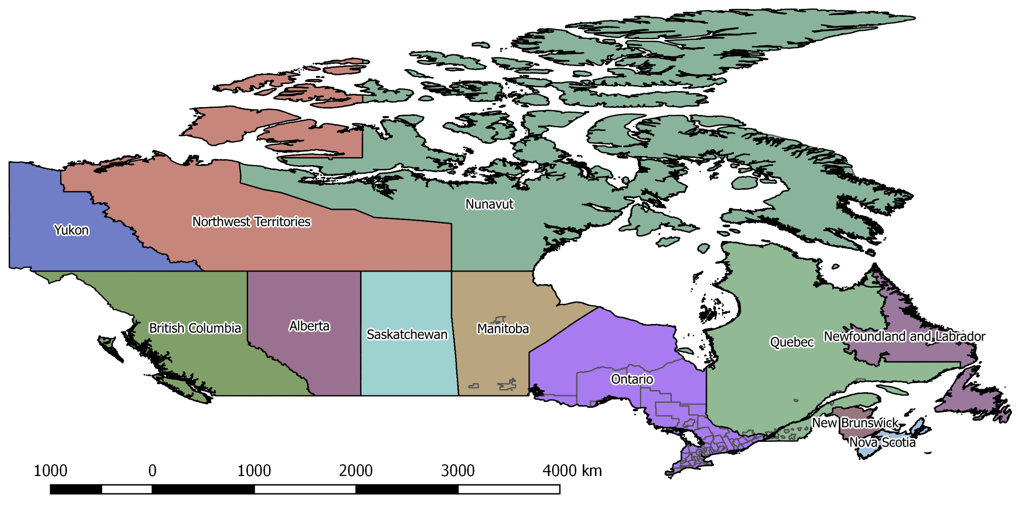
Since CMAs often overlap multiple census divisions, zones were defined by the union of the census division and CMA geometries. The resulting zone system had 69 internal zones for Ontario, the maximum number of destination choices discernible in the TSRC data. Using this approach, the distinction between urban and rural areas was encoded into the zone system. Interestingly, 51.5% of trips in the filtered TSRC survey originated from a CMA and 48.3% had a CMA destination. Both urban and regional areas contribute to long distance travel, with CMAs more likely to be origins than destinations. The final zone system used is presented in Figure 1.
The travel time, population and employment data was provided at the TAZ level by the project partner for the development of a larger statewide transport model. Each TAZ was assigned to the respective TSRC zone and the socioeconomic variables, namely, population and employment, summed for each zone. To aggregate the auto travel times between all TAZs to the zonal level, the travel time between each child origin–destination pair was weighted by the multiplied populations of the origin and destination.
where is the travel time between zones i; j, k, and l are TAZs belonging to zone j; and is the population in zone i.
This approach provides the benefits of considering the range of travel times that may exist between OD pairs. This was particularly important as in some of the larger regional zones, where the population centers are not centrally located. Travel times were available from a provincial transport model. Alternatively, travel times could be collected from Google Maps API (https://developers.google.com/maps/) or other online routing tools such as Graphhopper (https://github.com/graphhopper).
2.3. Foursquare
Foursquare collects a wealth of data on where and when users check-in. Data was collected using the Foursquare public venue API (https://developer.Foursquare.com/overview/venues.html). The API returns a list of venues in JSON format. Each venue record provides the following relevant information.
- Name
- Venue category
- Geo-referenced location
- Number of unique visitors
- Number of total check-ins
There are some limitations to the API. Each request is restricted to roughly 1 square degree of longitude and latitude in search area and only the top 50 venues for that search are returned, based on venue popularity. A limit of 5000 requests per hour is also enforced. Foursquare does not publish how the rank of returned venues is determined and the API does not return check-in counts by date. Hence, it could only be used to generate a total metric of activity for each venue, up to the time of the search. For the forecasting of trips to individual venues, this would present a significant obstacle. As such, the Foursquare metrics were only used for identifying the intensity of activity not reflected by socioeconomic variables.
The method to collect the venue data from the Foursquare API was as follows.
- A search grid of one degree raster cells was generated for the entire study area.
- A selection of potentially important venue categories was curated using the activities specified in the TSRC as a reference.
- To exclude Foursquare subcategories such as ‘States & Municipalities’, each category was mapped to at most five main Foursquare venue categories.
- The Foursquare API was queried for each cell and category, returning the top 50 venues, adhering to the rate limit of 5000 requests per hour.
- The resulting individual venues were stored in a PostGIS database and the number of check-ins for each category and zone were calculated (see Table 2).
- Duplicate venues were removed.In total, 34,041 unique venues and 7,981,458 check-ins were collected for the different categories.
3. Model Design
Defining Model Variables
Metropolitan areas are not homogeneous in land use patterns. Within urban areas, there are certain residential areas and central business districts to which people are more likely to travel. However, at the spatial resolution of the zone system these differences were hidden, resulting in a very high correlation between population and employment across the destination choice set of 98.95%. Therefore, we calculated a new variable for each destination j:
with population and employment .
Mishra et al. [16] found that interaction terms between the origin and the destination were significant for their destination choice model for Maryland. In a similar vein, three variables control for intra- and inter-zonal effects, where indicates that the zone is a CMA.
The first variable identifies trips within the same zone, where that zone is a metropolitan zone. This allows the model to reflect the propensity of a traveler to leave a metropolitan zone when they travel. The second, is 1 when the traveler is traveling from one metropolitan zone to another and 0 otherwise. This may be a common pattern for business travelers but is less likely for recreational trips. The third variable, , considers the intra-zonal behavior in larger, rural zones.
In discrete choice models that include distance or travel time terms in the form , it is common to include an additional parameter , giving . However, such exponential parameters can not be estimated without simulation.
To avoid the use of complex models from the GEV family [1], or trial and error methods, the for each model were taken from a previously designed gravity model, estimated with the same dataset as the discrete models in this paper (see [17]) for further details). The model results used are available in Table 3. This method produced good results, with an improved model accuracy and more significant travel time parameters than models tested without the parameter.
where is the number of trips produced in origin zone i, is the attraction at destination zone j, is the impedance factor, calibrated with the average trip travel time, and is the travel time between zones i, j.
For destination choice, multinomial logit models were used to calculate the probability of an individual in origin i with trip purpose k choosing a destination j from set .
This paper presents two multinomial logit models, A and B, to explore the usefulness of Foursquare-based alternative specific coefficients. The choice set of alternatives was the same for all individuals, containing all 69 zones within Ontario and the 48 external zones in Canada, giving a total of 117 alternatives. The same choice set and trip records were used for each model, meaning that the performance of each can be directly compared using the log likelihood metric as well as other metrics.
For model A, the utility function is the same for each trip purpose k.
In model B, separate utility functions for each trip purpose incorporate the relevant Foursquare categories. Hotels and sightseeing were included in all models, while medical was only considered for visit trips. Outdoor and skiing were considered for leisure trips in summer and winter, respectively. For leisure trips, an extra variable was included to capture the particular scenic attractiveness of Niagara falls.
4. Model Estimation and Results
This section discusses the estimation results of the destination choice models, shown in Table 4. The dataset was split into three categories, representing the three travel purposes: leisure, visit and business. In the first model iteration, model A, only the TSRC data was used to generate parameters.
The NRMSE considers the sample size of the estimation data by dividing the RMSE by the standard division of the observed values, to allow for the comparison of the model performance across trip purposes, despite their varying sample sizes. In terms of both the and normalized root mean square error (NRMSE), the results of this first model were good, particularly when compared to the singly-constrained gravity model estimated on the same dataset. However, the performance of the leisure sub-model was the weakest.
Furthermore, all parameters were highly significant and had the expected signs. The parameter signs and magnitude vary strongly across trip purposes. Business was the only purpose for which urban destinations were more likely to attract urban trips. On the other hand, leisure travelers were more likely to head for destinations outside the city. For visitation, there was a weak positive effect towards urban areas.
There was a strong negative effect of urban intra-zonal connections for all trip purposes, whereas for intra-zonal rural travel the effect was positive. This was as expected as urban areas are often too small to support long distance trips (those over 40 km). In rural zones, which are larger, the power law of travel distance means that long distance trips crossing into other zones are less likely [18]. The large negative coefficient for leisure intra-metro travel, combined with the other two origin–destination interaction parameters for leisure travel, suggest a strong preference for leaving urban areas for leisure. This is supported by the TSRC data, where the key leisure travel reasons include outdoor activities such as skiing, visiting national parks and camping.
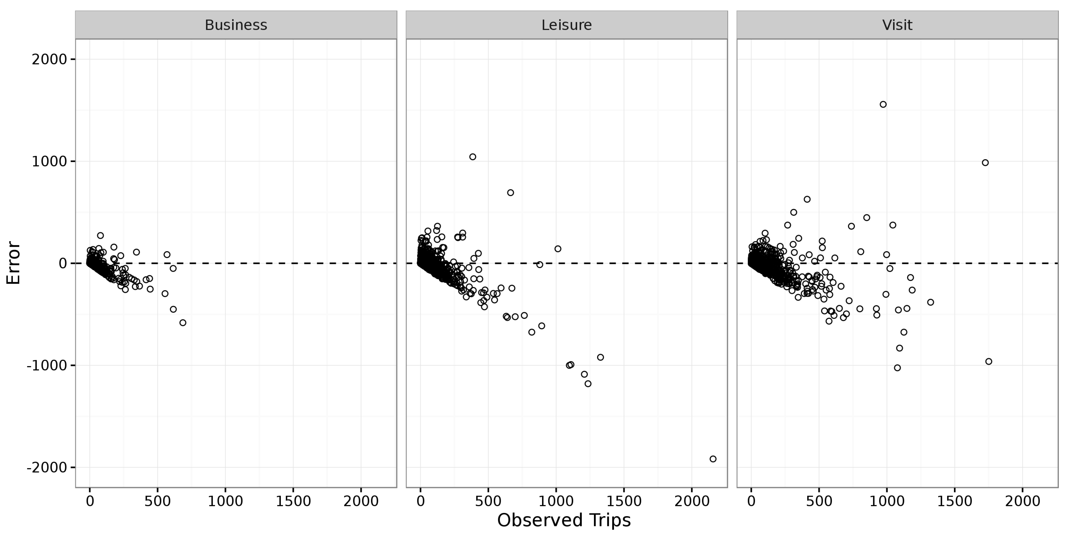
On closer inspection, the residuals graph in Figure 2 indicate that model A underestimated OD pairs with large numbers of trips and greatly overestimated some other smaller OD pairs. These sources of error fall into two categories:
- Overestimation of intra-zonal trips within metropolitan zones such as Toronto.
- Underestimation of leisure and visit trips from metropolitan centers to tourist attractions such as Niagara Falls.
In model B, certain categories based on Foursquare check-ins were found to be significant for particular trip purposes, i.e., the outdoor category for leisure trips and the medical category for visit trips. It is logical that the presence of hotels and sightseeing venues would be particularly important for leisure travel, and this was appropriately reflected in the coefficients in the model. The number of hotel check-ins was a significant variable across all trip purposes for long distance travel. Additionally, business conferences are often located in areas of significance to tourism as a way of promoting an event, supporting the large coefficient for sightseeing in the business category. The presence of medical facilities was found to be influential on the attractiveness of visit trip destinations. In model A, leisure trips to the zone containing Niagara Falls were underestimated by 85%. In model B, the Niagara variable controlled for this using the sightseeing category for leisure travel to the Niagara zone. Two variables, outdoors and skiing were found to be significant only for leisure travel in the season in which the respective activity is normally performed.
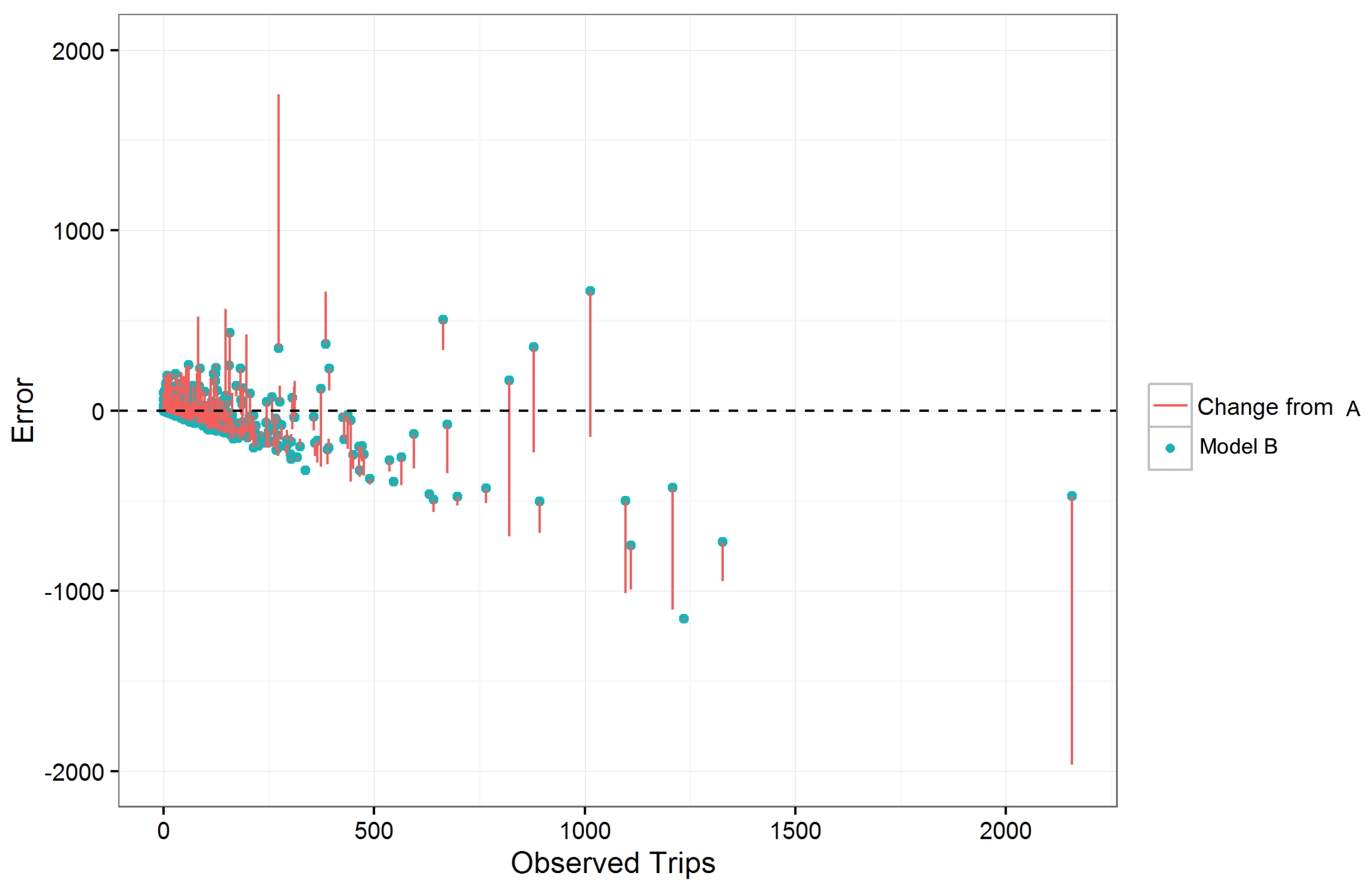
Overall, model B performed better across all trip purposes than model A, demonstrating the benefit of including the Foursquare based parameters. Particularly noticeable was the large improvement across all metrics for leisure travel. Figure 3 shows the impact of the Foursquare variables for leisure travel. While it is hard to visualize the impacts for smaller OD pairs, the graph illustrates how the errors for major OD pairs were reduced.
In both figures, there is a clear trend from the overestimation of trip counts for small OD pairs, to an underestimation as the number of observed trips increases. There are two reasons for the apparent trend. Firstly, there were 7819 OD pairs over the three trip purposes, with the majority having both very small trip counts and very small errors; 92% of the OD pairs had expected trip count of less than 100 and 99% of the residual error data points in Figure 3 are also less than 100. This significant skew means that the outliers, namely those that visualize a trend, constituted a very small portion of the dataset. Secondly, the trip count of an OD pair has a lower bound of zero but no upper bound. This lower bound is responsible for the linear lower limits observable in the residual graphs, Figure 2 and Figure 3. Fortunately, the trip counts were improved for both large and small OD by adding Foursquare data, as indicated by the vertical lines in Figure 3.
Scenario Analysis—Case Study of a New Ski Resort
This section presents a hypothetical application of the destination choice model. For any large scale land-use planning or development, it is important to model the impacts that such development would have on the transport network. As an example of this, a hypothetical scenario of the development of a large new ski resort was conducted. Ski resorts not only provide infrastructure for skiing and other snow-based activities but require the development of multiple new hotels, employee housing, and retail infrastructure. In the winter months, ski resorts place significant demands on the transport network that must be taken account when considering such a development.
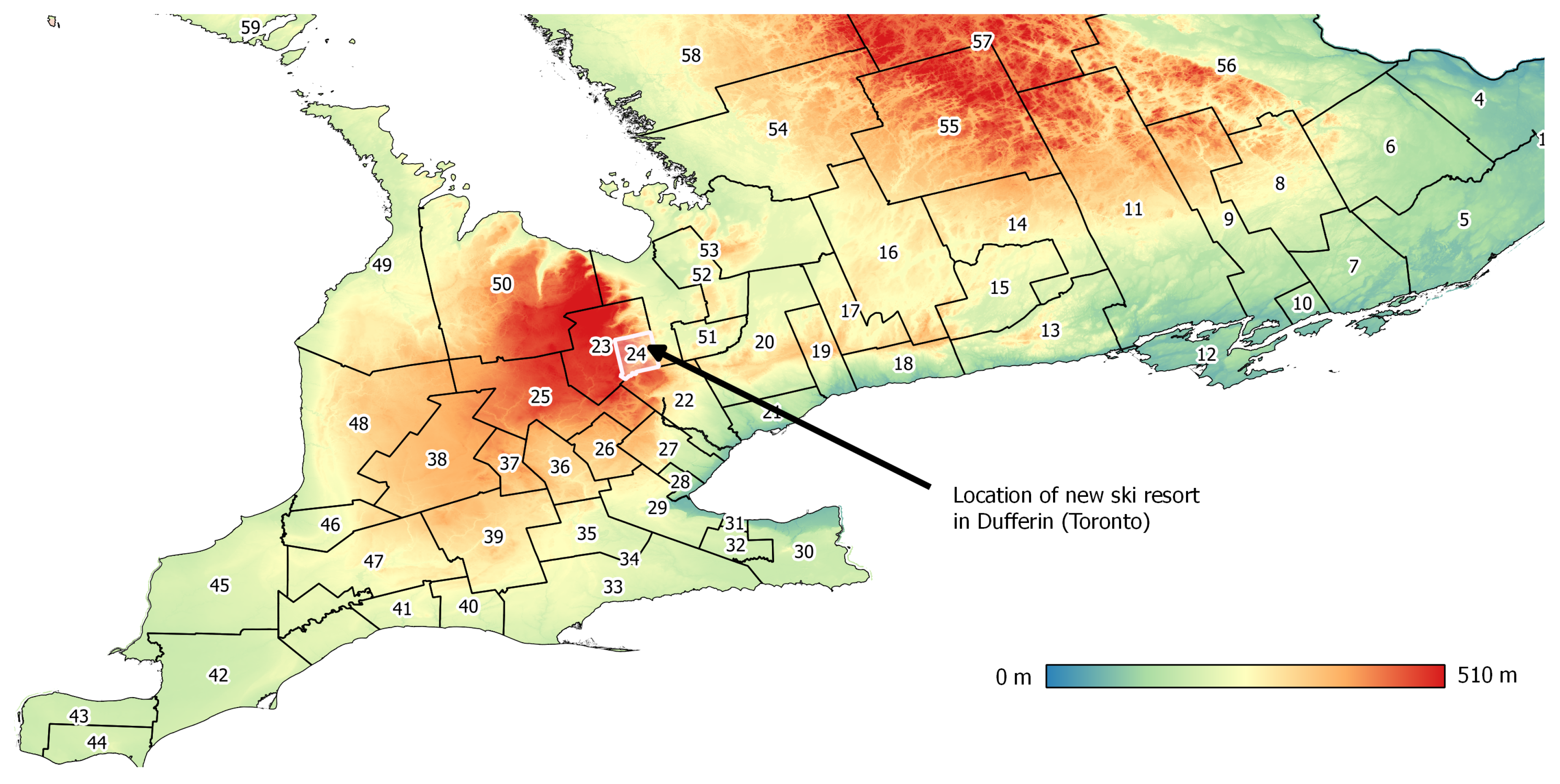
In the hypothetical scenario, a new resort is proposed for the highlands area north of Toronto in Dufferin (Toronto CMA) (see Figure 4). Its development is expected to bring similar numbers of visitors as other large resorts in Ontario. Three average sized hotels will also be built at the base of the resort to accommodate guests. In the summer, the resort will attract visitors by providing mountain biking facilities and hiking. Additional housing for 400 new residents are required to support 300 jobs. This scenario does not consider other policy and development considerations, such as site location and transport access. The impact of the new development was estimated by adjusting the hotels, skiing and outdoor variables for the zone in which the development will take place. The Foursquare POI database developed in Section 2.3 was used to estimate adjustments for each of the categories. Taking all venues in Ontario, the average number of check-ins per venue for each search category was calculated. The following adjustments were made for the respective zones and their values are displayed in Table 5.
- Skiing: The average number of check-ins for ski areas
- Hotel: Twice the average number of check-ins for hotels
- Outdoor: The average number of check-ins per outdoor venue
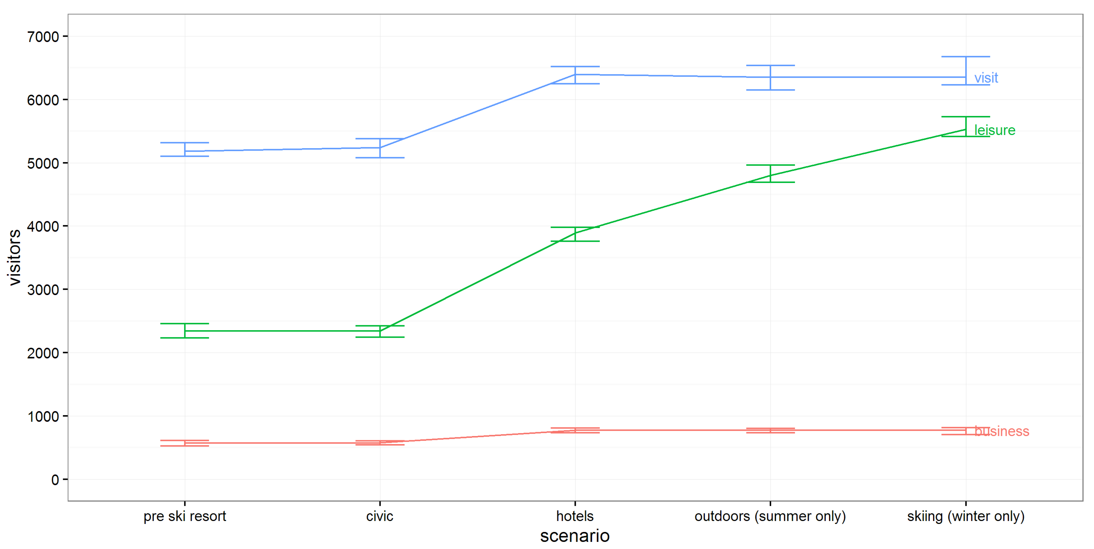
The trips from the TSRC data used for estimation were used as input to the scenario, with copies of each record added to the trip table, where w is the trip weight of the record. The weighted TSRC data represents the trip count over four years. For simplicity, the weights were scaled to give the approximate number of daily trips. Twenty iterations of the scenario were performed using a calibrated version of model B to account for the stochastic nature of destination choice. The calibration process was documented in [17]. Figure 5 shows the increase in incoming trips to Dufferin due to the new ski resort. The cumulative impact of each input is presented from left to right, with the rightmost column being the total impact of the combined parameters. The results show that the parameters behave reasonably. In particular the attractive effect for leisure travel is clearly visible. Without the Foursquare based parameters, the number of leisure trips would in fact decrease with the addition of a new ski resort, due to the negative coefficient of the variable in model A for leisure travel. This is a good example of why better representations of destination attractiveness are important, particularly for leisure travel.
5. Discussion
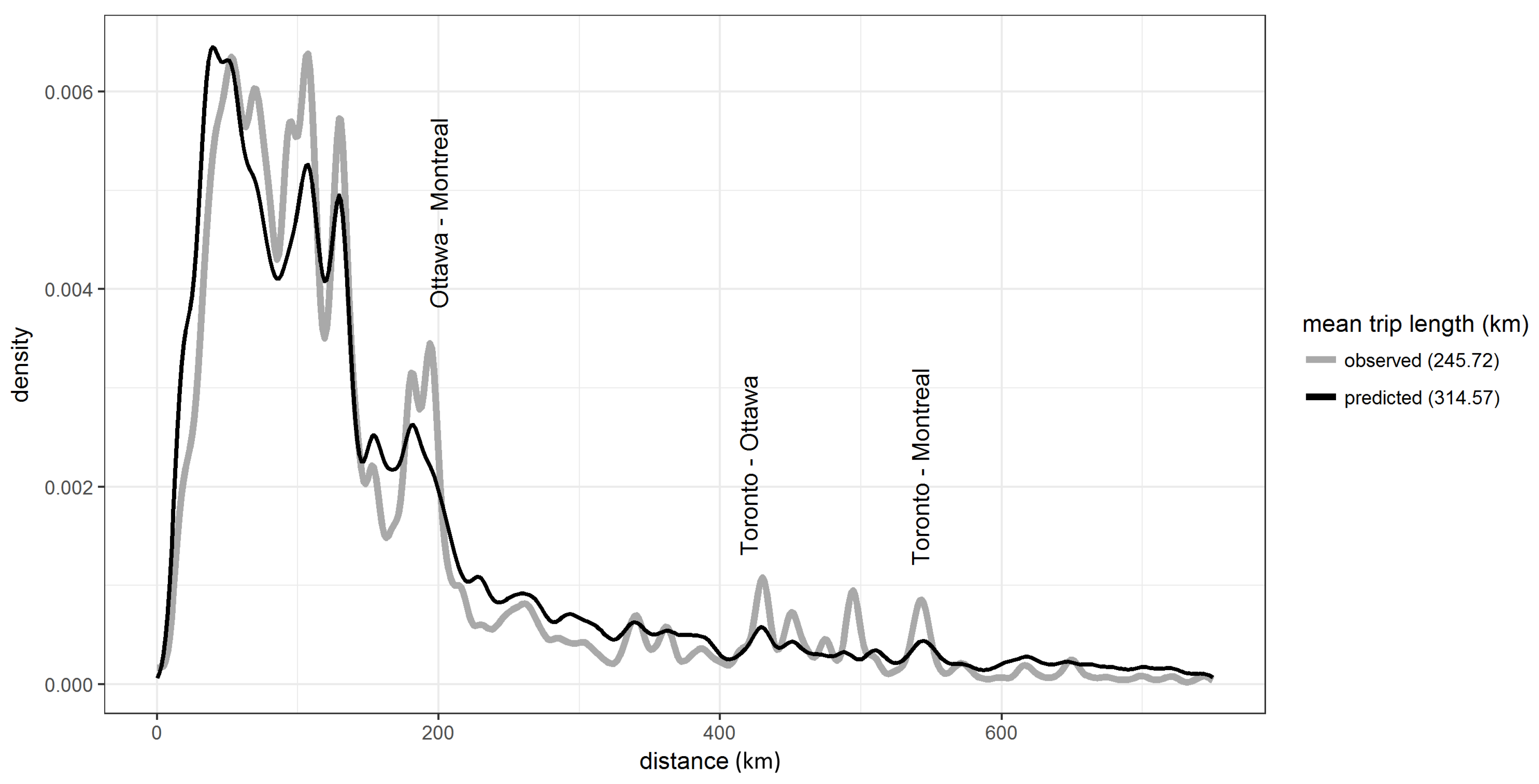
A closer inspection of the OD matrix generated by model B on the estimated data indicated the model still overestimated the number of intra-zonal trips within Toronto and underestimated the inter-zonal trips between large population centers, such as Toronto, Ottawa and Montreal. Figure 6 identifies the connections where the model falls short. The connections between the triangle of major cities, Toronto, Montreal and Ottawa are underestimated. The car journey from Toronto to Ottawa takes over four hours, while flying takes only 55 minutes. For this paper, only a skim matrix for car travel was available. The incorporation of travel times for all modes and the inclusion of feedback from the mode choice model, when available, would improve the estimation of these connections.
While there has been a ‘virtual explosion of data availability’ [19], Horni and Axhausen [20] note that the collection of big data such as GPS and GSM data “is generally associated with privacy, cost and technical issues”. These challenges go against the ideal of general models that are flexible and transferable [21]. Nonetheless, big data undoubtedly has a role to play in the future of transport modeling. Erath [22] suggests further research into probabilistic models based on big data and the blending of big data with data from travel diaries.
Venue data for each zone acted as database of the points of interest (POI) at a particular destination. POI data is available from many sources, such as Open Street Maps. However, LBSNs such as Foursquare take this POI database one step further, by measuring the popularity of each POI. In the case of Foursquare, check-ins measure the intensity of activity at each POI. A measure of importance is clearly beneficial in the model presented above, as not all POIs are equal; hotels are of different sizes and some national parks are more visited than others. Of course, the importance of each POI can be measured based on attributes such as the number of hotel beds or recorded visitors per year. However, the data collection required is prohibitive for most large scale models. LBSNs provides easily accessible data on the importance of individual POIs and, in turn, destination utility.
A mention must be made of the issue of model endogeneity. In reality, an increase in visits to a destination would most probably cause an increase in the number of check-ins. This leads to an endogeneity problem between the independent and dependent variables. One solution to avoid the endogeneity problem would be to use lagged variables, where the Foursquare check-ins are tallied from a period occurring before the TSRC data. Unfortunately, the public Foursquare API, at this time, does not allow the analyst to specify a time window. Hence, in this particular model, the endogeneity problem had to be accepted. Nonetheless, the work presented in this paper demonstrated the potential of such services to enhance our transportation models beyond the limitations of travel diaries and socioeconomic datasets.
Limitations and Future Work
One of the benefits of models based on socioeconomic variables is the ability to run the model for future years and model the impacts of demographic change. Forecasting the Foursquare check-in counts for different categories presents challenges to the modeler. Not only is it hard to predict how the popularity of certain venues will grow or decline in future years, but the quantity of check-ins depends on the uptake of the Foursquare platform and the potential emergence of competing platforms. Further study of the demographics of Foursquare users would help to define the statistical limitations of LBSN-based models. In future work utilizing more detailed Foursquare data, check-ins could be filtered for those performed only by residents of Canada or grouped by season to further improve the modeling of different trip purposes.
In study on why people use Foursquare, Lindqvist et al. [6] found that ‘participants expressed reluctance to check-in at home, work, and other places that one might expect them to be at’. This suggests that there are limits to how effectively Foursquare can model travel behavior. A potential alternative would be to take Foursquare or a similar LBSN as a POI database and use GPS traces to identify or impute the intensity of activity at these locations, thereby avoiding the selective reporting behavior evident in Foursquare usage.
6. Conclusions
In conclusion, this paper confirmed the hypothesis that aggregated geotagged big data can improve the modeling of destination choice when combined with traditional data sources. First, a zone system for long distance travel in Ontario, Canada was presented. Then, a methodology for the aggregation of historical Foursquare check-ins as indicators of destination attractiveness for particular categories was developed. Multinomial logit models were estimated to explore the potential of Foursquare check-ins for measuring destination attractiveness. The ‘traditional’ model based primarily on population, employment and zonal interactions was found to work well enough for visit and business travel but not leisure travel. With the addition of alternative specific parameters based on the Foursquare check-in data, the model accuracy across all trip purposes improved significantly, particularly for leisure travel. A scenario analysis using the expanded model further reinforced the importance of properly measuring destination attractiveness for leisure travel.
Acknowledgments
The research was completed with the support of the Technische Universität München—Institute for Advanced Study, funded by the German Excellence Initiative and the European Union Seventh Framework Programme under grant agreement n. 291763.
Author Contributions
The authors contributed equally to this work.
Conflicts of Interest
The authors declare no conflict of interest. The founding sponsors had no role in the design of the study; in the collection, analyses, or interpretation of data; in the writing of the manuscript and in the decision to publish the results.
References
- Train, K.E. Discrete Choice Methods with Simulation; Cambridge University Press: Cambridge, UK, 2009. [Google Scholar]
- Ben-Akiva, M.E.; Lerman, S.R. Discrete Choice Analysis: Theory and Application to Travel Demand; MIT Press: Cambridge, MA, USA, 1985; Volume 9. [Google Scholar]
- Simma, A.; Schlich, R.; Axhausen, K.W. Destination choice modelling of leisure trips: The case of Switzerland. In Working Papers Transport and Spatial Planning 99; Institute for Transport Planning and Systems, ETH Zurich: Zurich, Switzerland, 2001. [Google Scholar]
- Rashidi, T.H.; Abbasi, A.; Maghrebi, M.; Hasan, S.; Waller, T.S. Exploring the capacity of social media data for modelling travel behaviour: Opportunities and challenges. Transp. Res. Part C Emerg. Technol. 2017, 75, 197–211. [Google Scholar] [CrossRef]
- Issac, M. Foursquare Raises $45 Million, Cutting Its Valuation Nearly in Half, 2015. The New York Times. [Online]. 14 January 2016. Available online: https://www.nytimes.com/2016/01/15/technology/foursquare-raises-45-million-cutting-its-valuation-nearly-in-half.html (accessed on 14 August 2017).
- Lindqvist, J.; Cranshaw, J.; Wiese, J.; Hong, J.; Zimmerman, J. I’m the mayor of my house: examining why people use Foursquare-a social-driven location sharing application. In Proceedings of the SIGCHI Conference on Human Factors in Computing Systems, Vancouver, BC, Canada, 7–12 May 2011; ACM: New York, NY, USA, 2011; pp. 2409–2418. [Google Scholar]
- Cheng, Z.; Caverlee, J.; Lee, K.; Sui, D.Z. Exploring Millions of Footprints in Location Sharing Services. ICWSM 2011, 2011, 81–88. [Google Scholar]
- Rokib, S.A.; Karim, M.A.; Qiu, T.Z.; Kim, A. Origin-Destination Trip Estimation from Anonymous Cell Phone and Foursquare Data. In Proceedings of the Transportation Research Board 94th Annual Meeting, Washington, DC, USA, 11–15 January 2015. Number 15-2379. [Google Scholar]
- Noulas, A.; Scellato, S.; Lambiotte, R.; Pontil, M.; Mascolo, C. A tale of many cities: universal patterns in human urban mobility. PLoS ONE 2012, 7, e37027. [Google Scholar] [CrossRef]
- Stouffer, S.A. Intervening opportunities: A theory relating mobility and distance. Am. Sociol. Rev. 1940, 5, 845–867. [Google Scholar] [CrossRef]
- Hasan, S.; Ukkusuri, S.V. Reconstructing Activity Location Sequences From Incomplete Check-In Data: A Semi-Markov Continuous-Time Bayesian Network Model. IEEE Trans. Intell. Transp. Syst. 2017, PP, 1–12. [Google Scholar] [CrossRef]
- Beyer, M.A.; Laney, D. The Importance of ‘Big Data’: A Definition; Gartner: Stamford, CT, USA, 2012; pp. 2014–2018. [Google Scholar]
- Morstatter, F.; Pfeffer, J.; Liu, H.; Carley, K.M. Is the Sample Good Enough? Comparing Data from Twitter’s Streaming API with Twitter’s Firehose. In Proceedings of the Seventh International AAAI Conference on Weblogs and Social Media, Cambridge, MA, USA, 8–12 July 2013. [Google Scholar]
- Chaniotakis, E.; Antoniou, C.; Grau, J.M.S.; Dimitriou, L. Can Social Media data augment travel demand survey data? In Proceedings of the 2016 IEEE 19th International Conference on Intelligent Transportation Systems (ITSC), Rio de Janeiro, Brazil, 1–4 November 2016; pp. 1642–1647. [Google Scholar]
- Moeckel, R.; Donnelly, R. Gradual rasterization: Redefining spatial resolution in transport modelling. Environ. Plan. B Plan. Des. 2015, 42, 888–903. [Google Scholar] [CrossRef]
- Mishra, S.; Wang, Y.; Zhu, X.; Moeckel, R.; Mahapatra, S. Comparison between gravity and destination choice models for trip distribution in Maryland. In Proceedings of the Transportation Research Board 92nd Annual Meeting, Washington, DC, USA, 13–17 January 2013. [Google Scholar]
- Molloy, J. Development of a Destination Choice Model for Ontario. Master’s Thesis, Technical University of Munich, Munich, Germany, 2017. [Google Scholar]
- Gonzalez, M.C.; Hidalgo, C.A.; Barabasi, A.L. Understanding individual human mobility patterns. Nature 2008, 453, 779–782. [Google Scholar] [CrossRef] [PubMed]
- Nagel, K.; Axhausen, K.W. Workshop Report: Microsimulation. In The Leading Edge in Travel Behaviour Research; Hensher, D.A., Ed.; Pergamon: Oxford, UK, 2001; pp. 239–246. [Google Scholar]
- Horni, A.; Axhausen, K.W. How to Improve MATSim Destination Choice for Discretionary Activities? In Proceedings of the 12th Swiss Transport Research Conference, Ascona, Switzerland, 2–4 May 2012. [Google Scholar]
- Patriksson, M. The Traffic Assignment Problem: Models and Methods; Courier Dover Publications: Mineola, NY, USA, 2015; p. 6. [Google Scholar]
- Erath, A. Transport Modelling in the Age of Big Data; University of Seoul: Seoul, Korea, 2015. [Google Scholar]
Figure 1.
Zones by province for Canada.

Figure 2.
Model A: Errors by observed trip count for OD pairs by trip purpose.

Figure 3.
Effect of adding Foursquare variables in model B on leisure trip counts.

Figure 4.
Location of a new ski resort on Dufferin (Toronto CMA). Digits represent the zone ID. Elevation data from the Ontario Provincial Digital Elevation Model-Version 3.0.
Figure 4.
Location of a new ski resort on Dufferin (Toronto CMA). Digits represent the zone ID. Elevation data from the Ontario Provincial Digital Elevation Model-Version 3.0.

Figure 5.
Scenario analysis: Impact of a new ski resort on Dufferin (Toronto CMA).

Figure 6.
Trip length distribution of model B after calibration (0–750 km window).


Table 1.
Sample size by trip purpose.
| 2011 | 2012 | 2013 | 2014 | Total | |
|---|---|---|---|---|---|
| Business | 1798 | 1640 | 1449 | 1341 | 6228 |
| Leisure | 5939 | 5878 | 5515 | 5577 | 22,909 |
| Visit | 9057 | 8777 | 7962 | 7618 | 33,414 |
| Total | 18,694 | 18,016 | 16,547 | 16,071 | 69,328 |
Table 2.
Foursquare venue categories and totals.
| Category | Venue Categories | Venues | Check-ins |
|---|---|---|---|
| Medical | Dentist’s Office | 6294 | 586,082 |
| Doctor’s Office | |||
| Hospital | |||
| Medical Center | |||
| Veterinarian | |||
| Ski Area | Ski Area | 1048 | 203,266 |
| Ski Chairlift | |||
| Ski Chalet | |||
| Ski Lodge | |||
| Ski Trail | |||
| Hotel | Bed & Breakfast | 7268 | 1,502,248 |
| Hostel | |||
| Hotel | |||
| Motel | |||
| Resort | |||
| Outdoors | National Park | 7262 | 709,274 |
| Campground | |||
| Nature Preserve | |||
| Other Great Outdoors | |||
| Scenic Lookout | |||
| Sightseeing | Art Gallery | 4387 | 1,125,385 |
| Historic Site | |||
| Museum | |||
| Theme Park | |||
| Scenic Lookout | |||
| Total | 34,041 | 7,981,458 |
Table 3.
Gravity model calibration.
| Model | Trips | NRMSE | ||||
|---|---|---|---|---|---|---|
| Business | 34,229.43 | 244 | 243.20 | 0.0013 | 0.42 | 0.94 |
| Leisure | 83,357.94 | 149 | 148.13 | 0.0035 | 0.36 | 1.03 |
| Visit | 129,843.18 | 163 | 164.77 | 0.0030 | 0.52 | 0.93 |
Table 4.
Model estimation results (for all coefficients, ).
| Parameter | Visit | Leisure | Business | |||
|---|---|---|---|---|---|---|
| A | B | A | B | A | B | |
| 0.0013 | 0.0035 | 0.0030 | ||||
| 4.83 | 5.00 | 4.75 | 5.35 | 4.19 | 4.37 | |
| 0.57 | 0.21 | 0.52 | 0.76 | 0.36 | ||
| 0.56 | 0.72 | |||||
| 0.39 | 0.24 | 0.85 | 0.58 | 1.66 | 1.51 | |
| 0.11 | 0.27 | 0.17 | ||||
| 0.04 | 0.13 | 0.08 | ||||
| 0.13 | ||||||
| 0.03 | ||||||
| 0.10 | ||||||
| 0.07 | ||||||
| # Coefficients | 5 | 6 | 5 | 10 | 5 | 7 |
| Loglikelyhood | −115,666 | −114,557 | − 83,663 | −78,038 | −20,596 | −20,288 |
| AIC | 231,342 | 229,128 | 167,337 | 156,095 | 41,201 | 40,590 |
| 0.80 | 0.82 | 0.56 | 0.80 | 0.73 | 0.77 | |
| NRMSE (%) | 0.62 | 0.59 | 0.84 | 0.61 | 0.70 | 0.66 |
Table 5.
Inputs for scenario analysis.
| Parameter | Old Value | Adjustment | New Value |
|---|---|---|---|
| 42,216 | 700 | 42,916 | |
| 1393 | 8304 | 9697 | |
| 1 | 3389 | 3390 | |
| 40 | 3550 | 3590 |
© 2017 by the authors. Licensee MDPI, Basel, Switzerland. This article is an open access article distributed under the terms and conditions of the Creative Commons Attribution (CC BY) license (http://creativecommons.org/licenses/by/4.0/).
Share and Cite
MDPI and ACS Style
Molloy, J.; Moeckel, R. Improving Destination Choice Modeling Using Location-Based Big Data. ISPRS Int. J. Geo-Inf. 2017, 6, 291. https://doi.org/10.3390/ijgi6090291
AMA Style
Molloy J, Moeckel R. Improving Destination Choice Modeling Using Location-Based Big Data. ISPRS International Journal of Geo-Information. 2017; 6(9):291. https://doi.org/10.3390/ijgi6090291
Chicago/Turabian StyleMolloy, Joseph, and Rolf Moeckel. 2017. "Improving Destination Choice Modeling Using Location-Based Big Data" ISPRS International Journal of Geo-Information 6, no. 9: 291. https://doi.org/10.3390/ijgi6090291
Note that from the first issue of 2016, this journal uses article numbers instead of page numbers. See further details here.