Article

Predicting Modified Fournier Index by Using Artificial Neural Network in Central Europe

1
Institute of Land Use, Technical and Precision Technology, Faculty of Agricultural and Food Sciences and Environmental Management, University of Debrecen, 4032 Debrecen, Hungary
2
Institutes for Agricultural Research and Educational Farm, University of Debrecen, Böszörményi 138, 4032 Debrecen, Hungary
3
Department of Civil Engineering, College of Engineering, King Saud University, P.O. Box 800, Riyadh 11421, Saudi Arabia
4
Department of Transport Infrastructure and Water Resources Engineering, Széchenyi István University, Egyetem tér 1, 9026 Gyor, Hungary
5
Department of Civil Engineering, College of Ocean Science, Jeju National University, 102 Jejudaehakro, Jeju 63243, Korea
6
Department of Biosystems and Food Engineering, Faculty of Agricultural and Food Sciences, Széchenyi István University, Vár Square 2, 9200 Mosonmagyarovar, Hungary
7
Doctoral School of Humanities, University of Debrecen, Egyetem Tér 1, 4032 Debrecen, Hungary
*
Author to whom correspondence should be addressed.
Int. J. Environ. Res. Public Health 2022, 19(17), 10653; https://doi.org/10.3390/ijerph191710653
Submission received: 23 July 2022 / Revised: 16 August 2022 / Accepted: 20 August 2022 / Published: 26 August 2022

Abstract

:
The Modified Fournier Index (MFI) is one of the indices that can assess the erosivity of rainfall. However, the implementation of the artificial neural network (ANN) for the prediction of the MFI is still rare. In this research, climate data (monthly and yearly precipitation (pi, Ptotal) (mm), daily maximum precipitation (Pd-max) (mm), monthly mean temperature (Tavg) (°C), daily maximum mean temperature (Td-max) (°C), and daily minimum mean temperature (Td-min) (°C)) were collected from three stations in Hungary (Budapest, Debrecen, and Pécs) between 1901 and 2020. The MFI was calculated, and then, the performance of two ANNs (multilayer perceptron (MLP) and radial basis function (RBF)) in predicting the MFI was evaluated under four scenarios. The average MFI values were between 66.30 ± 15.40 (low erosivity) in Debrecen and 75.39 ± 15.39 (low erosivity) in Pecs. The prediction of the MFI by using MLP was good (NSEBudapest(SC3) = 0.71, NSEPécs(SC2) = 0.69). Additionally, the performance of RBF was accurate (NSEDebrecen(SC4) = 0.68, NSEPécs(SC3) = 0.73). However, the correlation coefficient between the observed MFI and the predicted one ranged between 0.83 (Budapest (SC2-MLP)) and 0.86 (Pécs (SC3-RBF)). Interestingly, the statistical analyses promoted SC2 (Pd-max + pi + Ptotal) and SC4 (Ptotal + Tavg + Td-max + Td-min) as the best scenarios for predicting MFI by using the ANN–MLP and ANN–RBF, respectively. However, the sensitivity analysis highlighted that Ptotal, pi, and Td-min had the highest relative importance in the prediction process. The output of this research promoted the ANN (MLP and RBF) as an effective tool for predicting rainfall erosivity in Central Europe.

1. Introduction

In many regions across the world, the most predominant type of land degradation is soil erosion, which has adverse environmental and socioeconomic consequences [1,2,3]. Soil erosion is the process of moving soil particles by external forces, such as mass movement, wind, and water [4,5]. In Europe, where a humid climate dominates, water-induced soil erosion is the main form of erosion, which poses a serious environmental concern in many European countries [6]. Furthermore, soil erosion by wind and dust storms is one of the challenges in European countries [7,8,9].
Soil erosion by water has numerous environmental impacts. For instance, detaching soil particles from the upper layer of the soil causes a deterioration in agriculture productivity through the loss of organic matter, nutrients, and soil depth [10]. Moreover, moving soil particles over vast distances affects the ecosystem service quality in downstream rivers by increasing the sedimentation and the contamination of aquatic life [11,12]. Since measuring soil erosion at a large scale is difficult, expensive, and time consuming, several models have been developed in recent decades to estimate soil erosion [13,14,15].
In Europe, the Universal Soil Loss Equation (USLE) [15], and its modified version, the Revisited Universal Soil Loss Equation (RUSLE) [14], is the most widely used in quantifying soil erosion at multiple scales across Europe. At large spatial scales, RUSLE is typically the most frequently used model to estimate soil erosion [16]. In the RUSLE model, the average annual soil erosion is calculated by multiplying six factors, including the rainfall erosivity factor (R factor). These factors are slope length (L-factor), soil erodibility (K-factor), slope steepness (S-factor), supporting conservation practices (P-factor), and crop type and management (C-factor). In this sense, rainfall erosivity is considered the most important, as rainfall has a direct impact on detaching and moving the soil particles [15].
Rainfall erosivity is the potential force of raindrops to detach and erode soil particles [17]. As it is one of the main causes of floods and landslides, researchers have highlighted rainfall erosivity as an important indicator to be investigated [18]. The rainfall erosivity factor is calculated using rainfall records with 1–5 min precipitation intervals [19]; however, these records are rarely accessible for long enough in most of the world. As a result, the kinetic energy concept has been widely employed to estimate the rainfall erosivity factor from half-hourly or hourly datasets [20].
To accurately estimate the R factor using the kinetic energy concept, it is necessary to measure both the intensity and the kinetic energy of the rain, but it is highly challenging to achieve this directly since the equipment needed is expensive and measuring the distribution of the rainstorm’s drop sizes is a tedious process [21]. To overcome this, researchers have developed numerous empirical equations that describe the relationship between rainfall intensity and its kinetic energy [22]. To provide a comprehensive review of these equations, Dash et al. [21] compared six of the most universal equations in more detail and provided a deep evaluation of their applicability in calculating the R factor. Alternative methods for calculating the R factor include index techniques, such as the Modified Fournier Index (MFI), especially when high-resolution rainfall records (half-hourly or hourly) are not available. The MFI is one of the methods suggested by Arnoldus [23] for calculating the R factor based on the monthly rainfall data. However, some adjustment is required for calculating the R factor based on the MFI result [24]. The MFI was used to estimate catastrophic erosion by evaluating rainfall erosivity and its association with other meteorological factors [25]. Previously, the MFI was implemented in many parts of the world, as can be seen in Table 1.
Recently, the artificial neural network (ANN) and machine learning algorithms have been widely used to predict environmental processes (erosion, contamination, and drought) in many parts of the world [29]. For instance, the multilayer perceptron neural network (MLPNN) model is one of the most widely used models for predicting hydrological data [30]. Mishra and Desai [31] used the ANN, RBF, and adaptive neural network-based fuzzy inference system (ANFIS) to forecast drought (SPI) at various timescales and found that ANN has better performance than RBF and ANFIS. In Iran, MLP, ANFIS, and multiple linear regression models were used for forecasting precipitation; the output showed that MLP produced better results [32]. Jalalkamali et al. [33] compared stochastic models with the ANN to forecast SPI-9 in Iran, and their results revealed that stochastic models performed better. The different model results depend on the drought index and its scale [34]. More examples of the implementation of the ANN for predicting certain environmental variables are presented in Table 2.
Based on the literature, few studies used the ANN to predict rainfall erosivity. However, limited information is available on MFI changes in Central Europe. Thus, the main goals of this research were to: (1) assess the Modified Fournier Index (MFI) as a representative for the erosivity index in three stations in Hungary between 1901 and 2020; (2) evaluate the ability of ANNs (multilayer perceptron (MLP) and the radial basis function (RBF)) to predict the MFI; and (3) rate the importance of input variables in predicting the MFI based on sensitivity analysis (∂). Overall, the implementation of ANN to predict MFI is still less common, which give this work novelty in its field, where the output will serve researchers, planners, and decision makers.

2. Materials and Methods

2.1. Data Collection

Data were collected from the Hungarian Metrological Center (https://www.met.hu/en/eghajlat/magyarorszag_eghajlata/eghajlati_adatsorok/Pecs/adatok/havi_adatok/, accessed on 1 June 2022). The data included the monthly rainfall (mm), daily maximum precipitation in the month (mm), monthly mean temperature (°C), daily maximum mean temperature in the month (°C), and daily minimum mean temperature in the month (°C) and were collected from three meteorological stations: Budapest (47°30′40′′ N, 19°01′41′′ E), Debrecen (47°29′44′′ N; 21°37′48′′ E), and Pécs (46°04’37′′ N, 18°13’29′′ E). Interestingly, the data cover 120 years from 1 January 1901 to 1 December 2020.

2.2. Modified Fournier Index (MFI)

Rainfall erosivity (R) represents the ability of rain drops to initiate erosion. To calculate the R factor, the measurement of rainfall intensity and rainfall duration is required [40]. As such data are not available in many places in the world, many indices were developed to determine the R factor. The Modified Fournier Index (MFI), which was proposed by Arnoldus [23], is a widely used index for estimating the R factor. The MFI is based on monthly precipitation (pi) and total yearly precipitation (Ptotal):
M F I = i = 1 i = 12 p i 2 P t o t a l
The output of Equation (1) can be categorized as presented in Table 3. Based on that, the MFI will have high values where the rainfall values are high. In this sense, regions with high amounts of total annual rainfall and rainfall precipitation concentration will have a high MFI value [41]. However, a strong correlation between MFI and R-factor was recorded in the literature [41,42]. Overall, the calculation of the MFI could provide a realistic estimation of the potential rainfall erosivity factor [43].

2.3. Predicting Rainfall Erosivity Based on Artificial Neural Network (ANN)

2.3.1. Thermotical Background of ANN Algorithms (MLP and RBF)

The artificial neural network consists of various interconnected neurons, nodes, or perceptrons that are called artificial neurons. Each node transmits a signal to another node; therefore, it can keep the information between various connections and distinguish the patterns [44]. The interconnected node obtains signals, processes them, and transforms them further. The transferring signal between nodes is a real number, and its output can be estimated using a nonlinear function by summing up all the inputs. The output of any network architecture works as an input for the preceding neuron [45,46].
There are several neural networks, but the multilayer perceptron (MLP) is widely used in environmental studies. The MLP connects nodes in a feedforward ANN. The MLP connections between nodes cannot form a cycle. The MLP is sometimes used as any feedforward ANN, and sometimes it refers to a network with various layers [47].
The MLP is a supervised learning technique used in backpropagation for training the dataset and has the ability to split the data that are not linearly separable. These attributes differentiate it from the linear MLP [48]. Ali et al. [49] used the MLP and found that it has the potential to predict drought as one of the ecosystem components in different performance measures. Therefore, in this study, we also used the MLP model. To estimate the y using a three-layer network with n number of neurons in the hidden layers and m number of inputs, we can use Equation (2):
y = f k = 0 n w j . g   i = 1 m   W j i   x i + w j 0 + w 0
Here, weight wj, joined with the jth neuron in the hidden layer and the output layer wji weight make a connection between the ith input variable and the jth neuron in the hidden layer, where xi is the ith independent variable, wj0 is the bias of the jth neuron, g is the activation function for the neuron of the hidden layer, and f is the activation function for the output layer [50].
The radial basis function (RBF) is another form of ANN, which was used in this research. The RBF was first proposed in 1988 by Broomhead and Lowe to solve the ill-conditioned problems in interpolation [51]. The RBF is a base of radial networks comprising neural network groups, i.e., a statistical neural network. Euclidean distance is the net input for the activation function of a neuron between its weight (w) and vector (i) multiplied by the bias b. The equation below (Equation (3)) presents the radial basis function network [50,52]:
a = 𝕝 w i 𝕝 b
Despite the differences between these two algorithms (i.e., MLP and RBF), both were used for predicting the MFI values in Central Europe.

2.3.2. Modeling Framework

Input Variable

Based on Equation (1), the only necessary data for calculating the MFI is rainfall data (pi and Ptotal). However, for the modeling approach, we engaged other climatic factors, including the daily maximum precipitation (mm) (Pd-max), monthly mean temperature (°C) (Tavg), daily maximum mean temperature (°C) (Td-max), and daily minimum mean temperature (°C) (Td-min). An overview of the input variable for each station is presented in Figure 1 and Figure 2 and Table 4.
For the modeling approach, five scenarios were adopted, as can be seen in Table 5. The main purpose of adopting different scenarios is to assess the function of the ANN (MLP and RBF) in predicting the MFI based on different input variables. For instance, the first scenario includes all input variables (rainfall (daily + monthly + total) + temperature (monthly)), while the last scenario includes only two rainfall parameters.

Training, Testing, and Sensitivity Analysis for Different ANN (MLP and RBF) Algorithms

For the five implemented scenarios and ANN (MLP and RBF) algorithms, data were divided randomly into 70% for training and 30% for testing. As this work was conducted in an SPSS environment, the initial conduction for each algorithm was adopted. For instance, the number of layers of hidden units was from 1 to 50, and the training type was Batch (initial Lambda = 0.000005) for the MLP algorithm, while the architecture of the RBF algorithm was based on automatically finding the number of units in the hidden layer with the normalized RBF as an activation function.
Finally, sensitivity analysis (∂) was used to highlight the relationship between the input variable for each scenario and the predicted MFI, as shown in Figure 3.

Assessing the ANN Performance

To assess the performance of the ANN algorithms (MLP and RBF) in predicting the MFI, four indices were used. The indices are model efficiency (NSE) [53], index of agreement correlation (d) [54], root mean square error (RMSE) [55], and Pearson correlation coefficient (r) [56], as shown in Table 6.
Additionally, the Taylor diagram [57] was used to plot the M F I C a l against M F I P r d . In this sense, the Taylor diagram provides a full overview of the best model/scenarios (Table 5) based on the correlation and standard deviation.
Finally, it is important to mention that all input and output along with the modeling approach was conducted in IBM SPSS Statistics (V. 24). The SPSS was chosen as it provides a user-friendly platform along with a variety of options that could optimize the output and ANN algorithm. However, we used the initial recommended sets (i.e., batch is the type of training, initial Lambda is 0.0000005, initial Sigma is 0.00005) by SPSS for conducting the modeling.

3. Results

3.1. MFI Variability in Hungary

In the three studied stations, the MFI follows a normal distribution (Figure 4). The average MFI values were between 66.30 ± 15.40 (low erosivity) in Debrecen and 75.39 ± 15.39 (low erosivity) in Pecs (Table 7). In Budapest (central Hungary), the highest MFI (129.17, high) value was recorded in 1955, which corresponds to 898.8 mm of rainfall, while the lowest MFI value (37.21) was recorded in 1997. In Debrecen (eastern Hungary), the highest MFI value was 126.23 (high) in 1977. However, the maximum MFI value in Pecs (southern Hungary) was 121.09 (high) in 1972. Interestingly, the highest frequency of the MFI values was 31 in Budapest, 29 in Debrecen, and 24 in Pecs for the values (65.04, 74.32), (54.28, 63.37), and (81.41, 89.53), respectively (Figure 4).

3.2. MFI Prediction by ANN–MLP and ANN–RBF

In the three stations, a combination of different climate variables (four scenarios) was used by ANN–MLP and ANN–RBF for predicting the MFI values. The predicted MFI values are presented in Figure 5 and Figure 6.
For the ANN–MLP, each scenario exhibited a different performance in predicting MFI values (Figure 5). In Budapest, the Pearson correlation coefficient (r) ranged between 0.82 (SC1-MLP) and rMFI vs. MFI prd = 0.83 for the rest of the scenarios. The d index ranged between 0.88 (SC1-MLP) and 0.9 (SC3-MLP). The efficiency of the ANN–MLP was assessed using the NSE. However, the NSE value was above 0.6, which indicates a good model performance for all scenarios. However, the highest value was NSE = 0.7 in SC3. Interestingly, the highest NSE value and lowest RMSE were recorded in SC3. Based on the statistical indicator, the efficiency of the scenarios in predicting the MFI can be highlighted as follows: SC3 > SC2 > SC4 > SC1. For Debrecen, the ANN–MLP exhibited a good performance (Figure 7). The r values and those of other statistical indicators were lower than those recorded in Budapest. For instance, the r ranged between 0.79 and 0.81, and the NSE between 0.62 and 0.66, while the RMSE was higher than Budapest. Based on the four suggested scenarios, the ANN–MLP performance could be ranked as follows: SC1 > SC2 > SC4 > SC3. Similar to Budapest, the ANN–MLP performance in Pecs was better than that in Debrecen (Figure 7). The d index was higher than 0.88, and the NSE was good (NSE > 0.66). Based on this, we can draw the following rank: SC2 > SC3 > SC1 > SC4.
Similar to ANN–MLP, the ANN–RBF showed a good ability to predict the MFI under different scenarios (Figure 6). In Budapest and Debrecen, SC4 had the highest correlation rMFI vs. MFI prd (0.85, 0.82), with the highest and lowest NSE, respectively, which indicates that SC4 (ANN–RBF) (pi + Ptotal) is the best scenario for Budapest and Debrecen. In this sense, the scenarios can be ranked for both stations as follows: SC4 > SC2 > SC3 > SC1 (Figure 7). In Pecs, SC3 (ANN–RBF) (Ptotal + Tavg + Td-max + Td-min) outperformed the rest of the scenarios (rMFI vs. MFI prd = 0.86, d = 0.92, NSE = 0.73, RMSE = 7.8). However, the performance of the four scenarios can be ranked as SC3 > SC4 > SC2 > SC1.
The Taylor diagram (Figure 8) reveals that SC2 and SC3 for Budapest and SC1 and SC2 for Debrecen and Pecs are the best scenarios in terms of the ANN–MLP (Figure 8). However, for the ANN–RBF, SC4 was the most appropriate scenario for Budapest and Debrecen, while SC3 was the best one for Pecs. Overall, these analyses promoted SC2 (Pd-max + pi + Ptotal) and SC4 (Ptotal + Tavg + Td-max + Td-min) as the best scenarios for predicting MFI using the ANN–MLP and ANN–RBF, respectively.

3.3. Comparing between ANN–MLP and ANN–RBF in MFI Prediction

To compare the outputs of each algorithm in each station, the outputs were plotted in a Taylor diagram (Figure 9). The main point of this step is to test all the scenarios for both algorithms against the calculated MF. For Budapest and Debrecen stations, the RBF-SC4 followed by the MLP-SC2 was the best predictor. In Pecs, the RBF-SC3 followed by the MLP-SC1 was superior compared to the others. Notably, in the three stations, the RBF-SC1 had the worst performance (Figure 9). Interestingly, the RBF outperformed the MLP.

3.4. Independent Variable Importance and Sensitivity Analysis

The main goal of sensitivity analysis is to highlight the importance of the input variables in the prediction process. For the MLP in the Budapest station, the Ptotal had the highest importance in all the suggested scenarios (∂SC1 = 0.46; ∂SC2 = 0.86; ∂SC3 = 0.79; ∂SC4 = 0.95), followed by Tavg in SC1, and Td-min in SC3 (Figure 10). For the RBF in the same station, the Ptotal also had the highest importance (∂SC1 = 0.45; ∂SC2 = 0.64; ∂SC3 = 0.44; ∂SC4 = 0.88). However, other independent variables exhibited a good level of importance. For example, in SC1 Td-min, Td-max and pi showed ∂SC1 importance ranging between 0.13 and 0.11, while in SC2, the pi importance reached ∂SC2 = 0.2 (Figure 10).
For the second station (Debrecen), both algorithms showed that Ptotal has an important role in MFI prediction. In the MLP, the importance value reached ∂SC4 = 0.73, while it was ∂SC4 = 0.82 in the RBF. Notably, the next important variable was the pi, with ∂SC2-MLP = 0.24 and ∂SC2-MLP = 0.22. At the Pecs station, the importance of the Ptotal was more pronounced for both the MLP (∂SC4 = 0.97) and RBF(∂SC4 = 0.83) (Figure 10).
Based on the four scenarios and both ANN (MLP and RBF) algorithms, the sensitivity analysis showed that Ptotal, pi, and Td-min had the highest relative importance in the prediction process.

4. Discussion

In this research, the MFI was calculated for tracking rainfall erosivity in Central Europe; then, two ANN (RBF and MLP) algorithms were tested to assess their ability in the prediction of the 
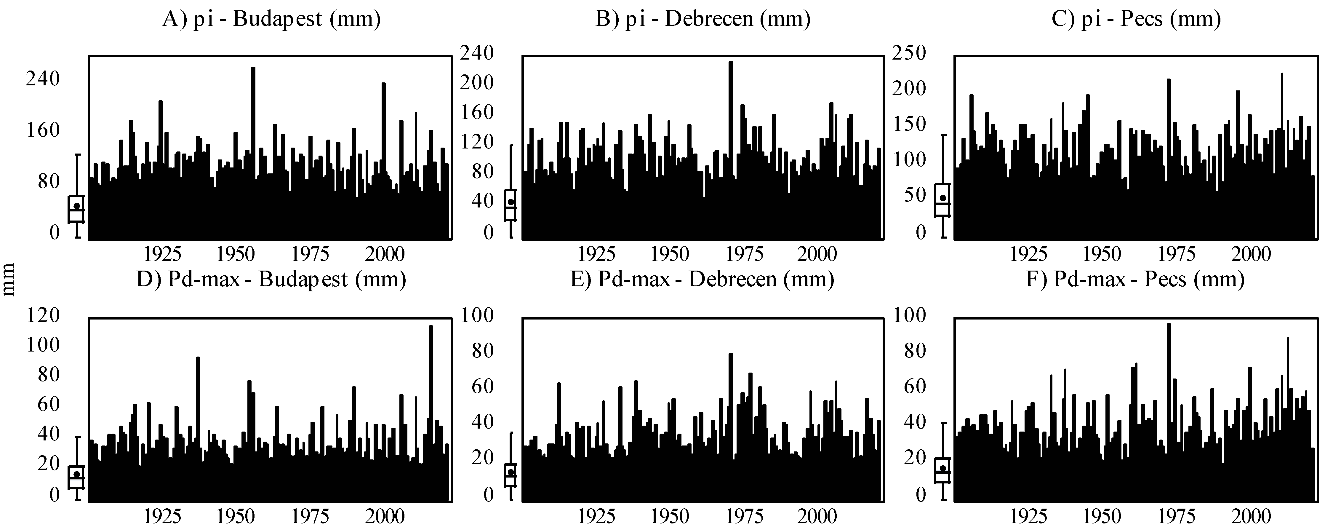
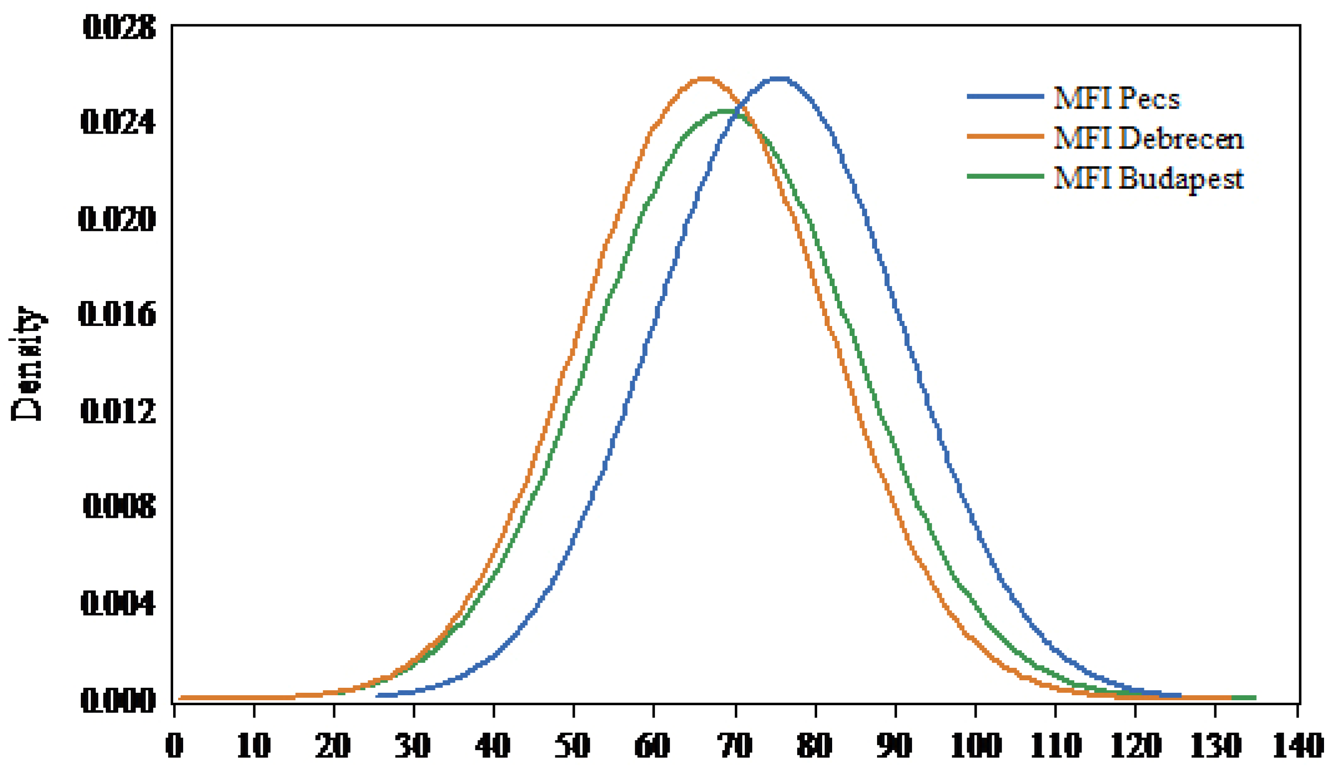
MFI. At the three studied stations, the MFI values ranged from very low to high (1901–2020) (Table 7). Previously, De Luis et al. [41] analyzed the erosivity trend in Western Europe (Iberian Peninsula) and detected a notable decrease in rainfall erosivity based on the MFI (1951–2000). For the Netherlands, Lukić et al. [10] reported that the MFI values ranged between 77.93 and 97.27 (1957–2016). However, changes in erosivity class from low to moderate were reported in the same study. These changes in rainfall erosivity in Europe can be mainly explained by climate change (i.e., extreme events: flood and drought), which largely affects the precipitation patterns, not only in Europe but all over the world [58,59,60,61].
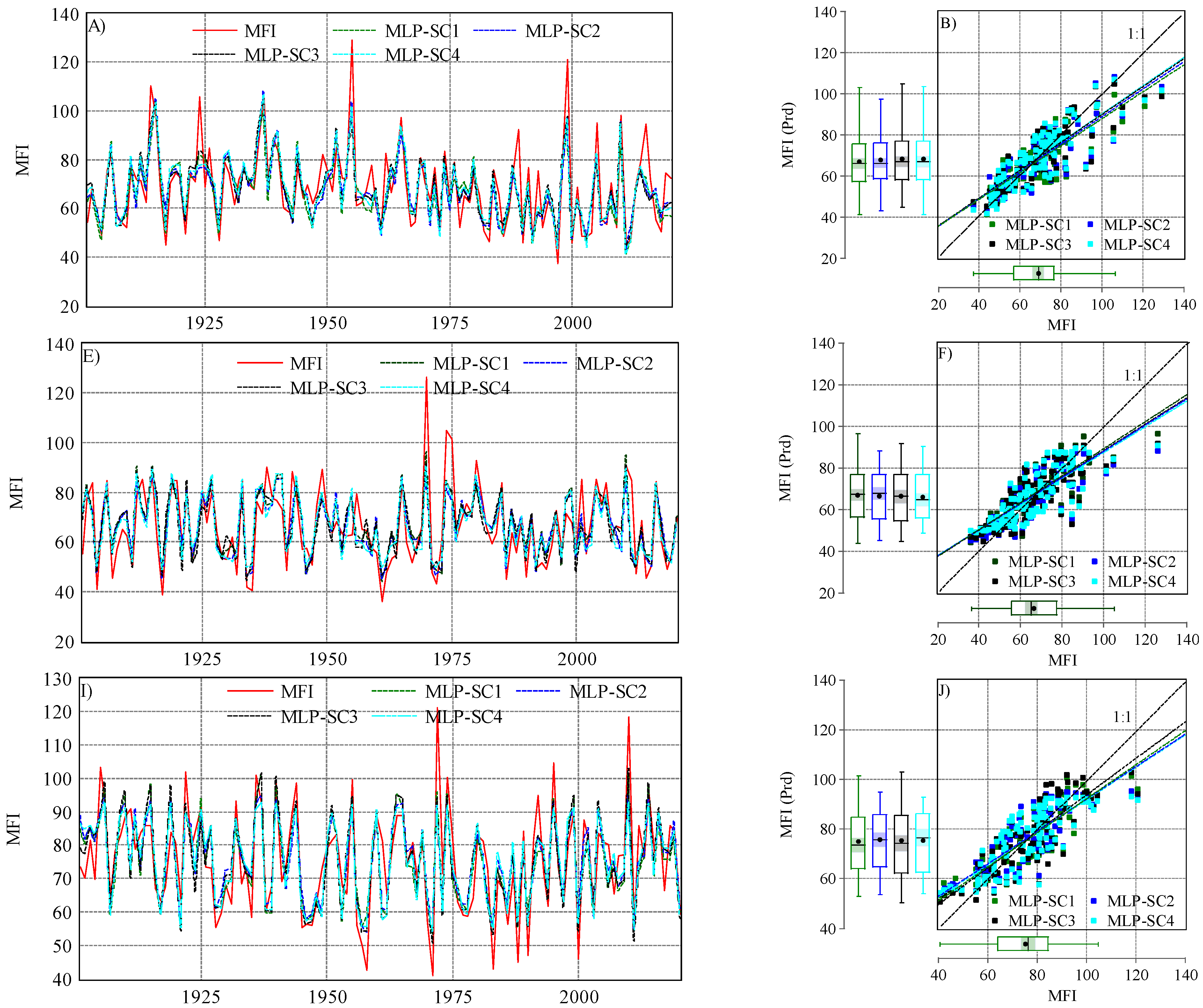
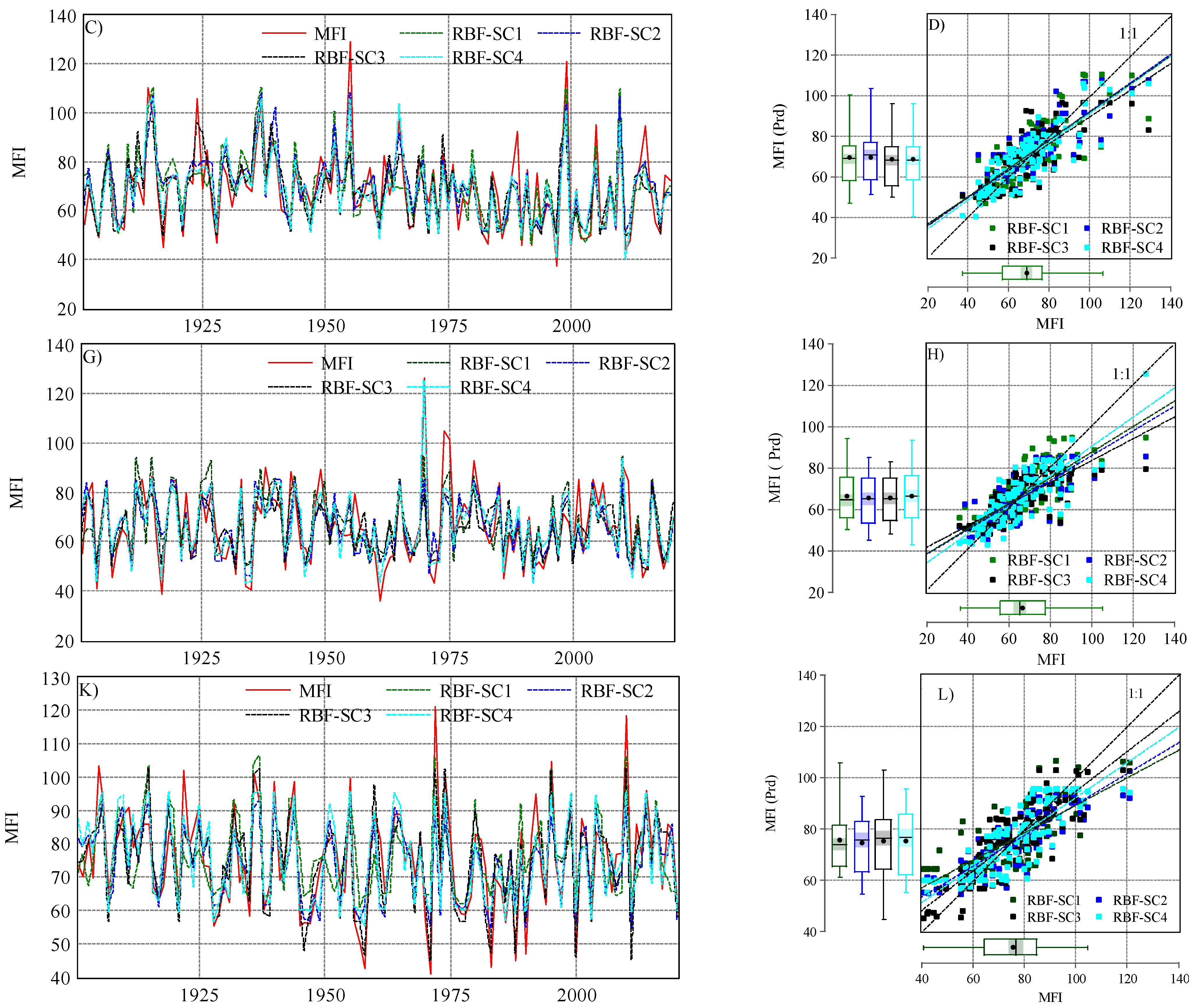
The output of RBF and MLP showed that the RBF outperformed the MLP. However, both algorithms were perfectly capable of predicting the MFI values, with some differences. The differences between the output could be explained by the way that each algorithm works. The necessary step for the proper functioning of the NN is to optimize the weights, known as calibration. Different types of algorithms can be used to optimize the weight, e.g., back propagation [62] and Levenberg–Marquardt [63]. These algorithms can minimize the disparity between forecasted and observed values by adjusting the network weight [46].
Generally, the ANN works on the principle of the training dataset. There are various kinds of neural network (NN) models, but usually, two models are used in prediction applications, i.e., recurrent network and feedforward network. The backpropagation algorithm is used to train both models [49,50,51,52,53,54,55,56,57,58,59,60,61,62,63,64]. When the backpropagation algorithm is used to change the weight of neurons, it works on the gradient descent method (weights change in downward direction). The signal strength between nodes is directly dependent on the weights of neurons [49]. Feedforward NN is a basic type, and it is capable of estimating constant and integral functions.
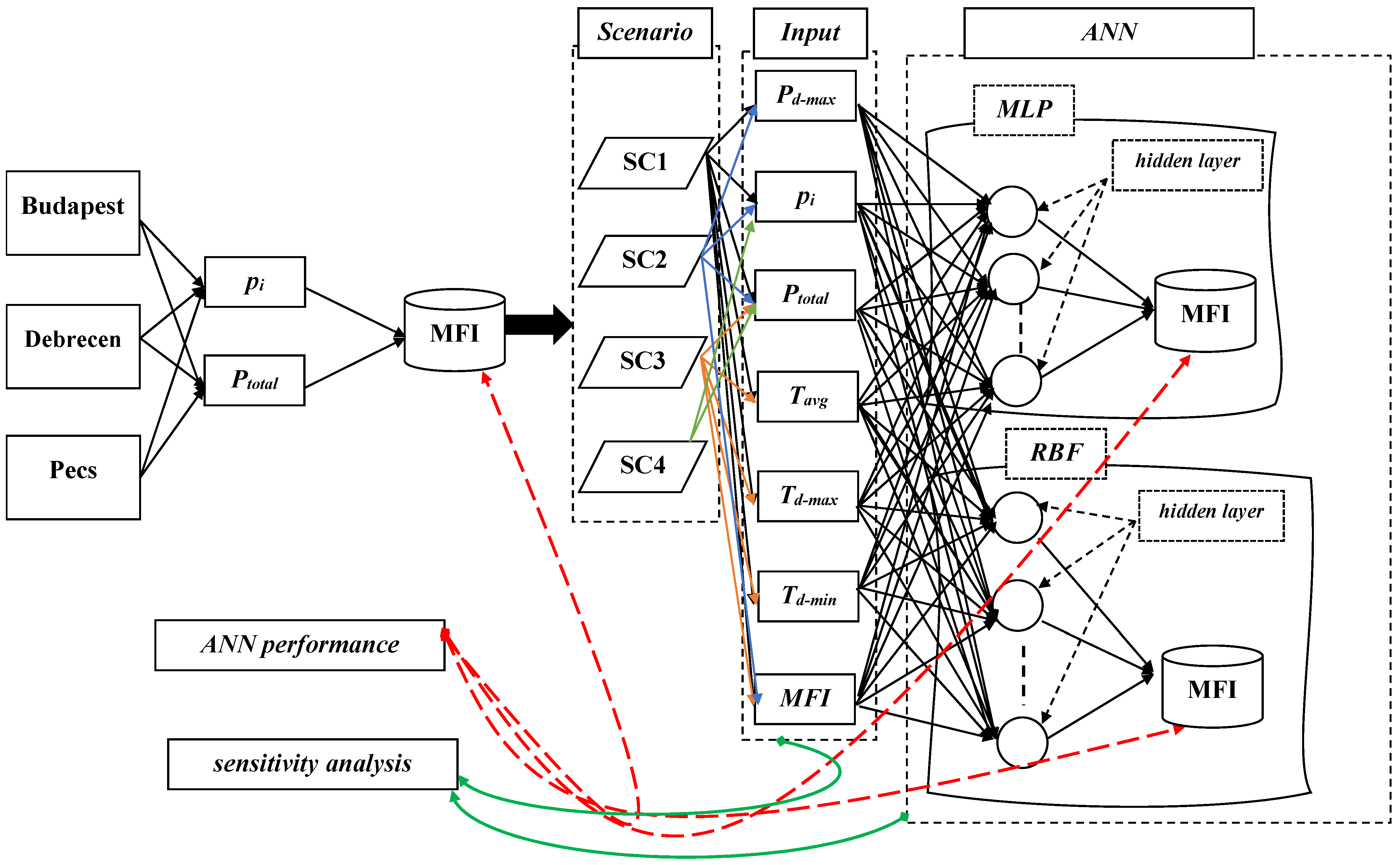
The network architecture of MLP comprises neurons put together into layers. The MLP contains three layers of nodes, i.e., input, hidden, and output layers. The MLP can have one or more hidden layers with various numbers of neurons. In addition to the input node, the hidden and output nodes are considered neurons [65]. When we used the MLP to study rainfall erosivity (MFI), the input layer contained the variables (Pd-max, pi, Ptotal, Tavg, Td-max, and Td-min), and the output layer presented the predicted MFI (Figure 3), while the hidden layer included a nonlinear function and utilized weight for the input layer. Neurons in the hidden layer work in a trial and error approach [34].
The MLP and RBF consist of three network layers; however, the main difference between the RBF and MLP is that the RBF’s hidden and output layers are different, unlike those of the MLP [66]. The hidden layer neurons are nonlinear, while the output layer neurons are linear in the RBFs. The nonlinear hidden layer neuron plays a significant role in the nonlinear modeling task [67]. The RBF network is simpler compared to MLP. However, the MLP is more successfully implemented in various complex problems. The RBF is a local approximation network, and its output can be estimated by hidden units in a local receptive field. The MLP network works globally, and its output is determined by all the neurons [
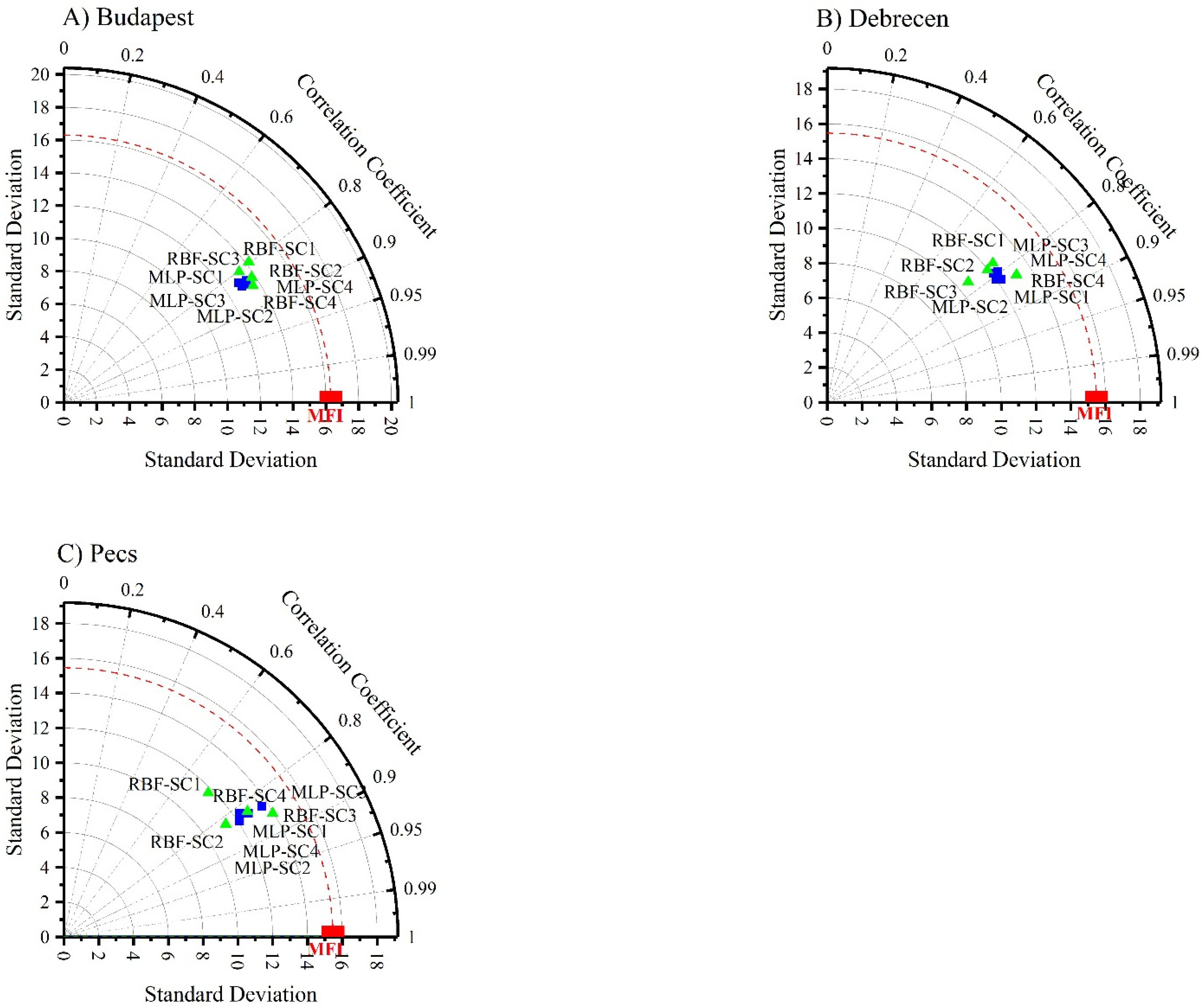
68]. Despite the similarity between both algorithms, the differences in the architecture process led to different output and accuracy (Figure 7, Figure 8 and Figure 9).
Overall, the implementation of the ANN for predicting the MFI or other hydrological and environmental variables was proven to be a useful tool for predicting and forecasting [69]. However, the output of this research could be useful for local planners on a county scale for predicting the MFI values based only on monthly and yearly rainfall.

5. Conclusions

Land degradation is a major issue all over the world due to its negative impact on the agroecosystem and environmental components. Recently, machine learning and the artificial neural network have been implemented in environmental research for predicting natural hazards. In this research, ANN (MLP and RBF) algorithms were implemented to predict the MFI as a representative of erosivity factor (soil erosion) in Central Europe. Five scenarios with different inputs (rainfall and temperature) were suggested for exploring the accuracy of ANN (MLP and RBF) algorithms. The output of this research can be summarized as follows:
1-
The MFI ranged between 91.97 (Budapest) and 80.25 (Pecs), with a notable decrease in MFI values (1901–2020).
2-
The SC2 (Pd-max + pi + Ptotal) was the best scenario for predicting the MFI using the ANN–MLP.
3-
The SC4 (Ptotal + Tavg + Td-max + Td-min) was the most accurate scenario for predicting the MFI by using the ANN–RBF.
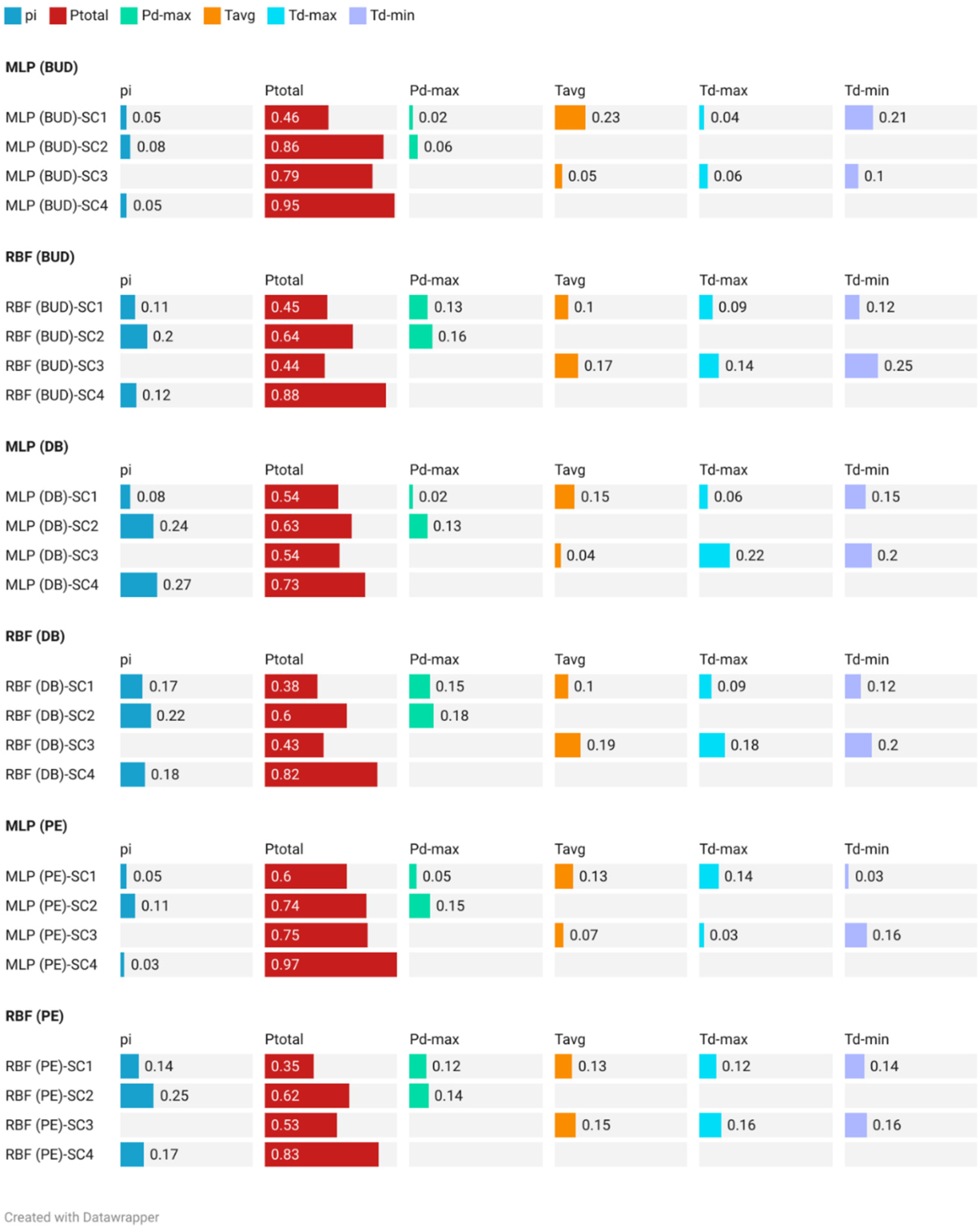
4-
The sensitivity analysis revealed that pi followed by Ptotal are the most important input variables for predicting MFI values.
It is good to mention that this research was only focused on MFI as one of the factors that contribute to soil erosion based on the monthly rainfall data. Some other factors such as land use (agricultural areas), soil properties (i.e., texture, structure), vegetation cover, and inclination angle of rainfall streams were not considered in this research.
Local planers, environmental organizations, and decision makers will be able to use the output of this research, where the prediction of the MFI could be performed to a satisfactory level based on the total rainfall in the target regions. In the next steps, other machine learning methods will be implemented to test their accuracy in the prediction of the MFI. However, the output of this research could serve as a good result for both scientific and industrial communities.

Author Contributions

Conceptualization: S.M. and E.H.; writing—original draft: S.M.; methodology: S.M.; writing—review and editing: F.A., M.F.U.M., A.S., I.T., B.B., A.A., T.R., A.N. and E.H. All authors have read and agreed to the published version of the manuscript.

Funding

Project no. TKP2021-NKTA-32 was implemented with the support provided by the National Research, Development, and Innovation Fund of Hungary, financed under the TKP2021-NKTA funding scheme. This research was supported by the RESEARCHERS SUPPORTING PROJECT, grant number RSP-2021/296, King Saud University, Riyadh, Saudi Arabia.

Institutional Review Board Statement

Not applicable.

Informed Consent Statement

Not applicable.

Data Availability Statement

Acknowledgments

The authors would like to thank Debrecen university for their unlimited support.

Conflicts of Interest

The authors declare no conflict of interest.

References

  1. Luetzenburg, G.; Bittner, M.J.; Calsamiglia, A.; Renschler, C.S.; Estrany, J.; Poeppl, R. Climate and land use change effects on soil erosion in two small agricultural catchment systems Fugnitz–Austria, Can Revull–Spain. Sci. Total Environ. 2020, 704, 135389. [Google Scholar] [CrossRef] [PubMed]
  2. Mohammed, S.; Al-Ebraheem, A.; Holb, I.J.; Alsafadi, K.; Dikkeh, M.; Pham, Q.B.; Linh, N.T.T.; Szabo, S. Soil management effects on soil water erosion and runoff in central Syria—A comparative evaluation of general linear model and random forest regression. Water 2020, 12, 2529. [Google Scholar] [CrossRef]
  3. Mohammed, S.; Alsafadi, K.; Talukdar, S.; Kiwan, S.; Hennawi, S.; Alshihabi, O.; Sharaf, M.; Harsanyie, E. Estimation of soil erosion risk in southern part of Syria by using RUSLE integrating geo informatics approach. Remote Sens. Appl. Soc. Environ. 2020, 20, 100375. [Google Scholar] [CrossRef]
  4. Bullock, P. Climate Change Impact. In Encyclopedia of Soils in the Environment; Cranfield University–Silsoe: Silsoe, UK, 2005; pp. 254–262. [Google Scholar] [CrossRef]
  5. Mohammed, S.; Hassan, E.; Abdo, H.G.; Szabo, S.; Mokhtar, A.; Alsafadi, K.; Alsafadi, K.; Al-Khouri, I.; Rodrigo-Comino, J. Impacts of rainstorms on soil erosion and organic matter for different cover crop systems in the western coast agricultural region of Syria. Soil Use Manag. 2021, 37, 196–213. [Google Scholar] [CrossRef]
  6. Panagos, P.; Katsoyiannis, A. Soil erosion modelling: The new challenges as the result of policy developments in Europe. Environ. Res. 2019, 172, 470–474. [Google Scholar] [CrossRef]
  7. Hojan, M.; Rurek, M.; Więcław, M.; Krupa, A. Effects of extreme dust storm in agricultural areas (Poland, the Greater Lowland). Geosciences 2019, 9, 106. [Google Scholar] [CrossRef]
  8. Szczepanik, D.M.; Ortiz-Amezcua, P.; Heese, B.; D’Amico, G.; Stachlewska, I.S. First Ever Observations of Mineral Dust in Wintertime over Warsaw, Poland. Remote Sens. 2022, 14, 3788. [Google Scholar] [CrossRef]
  9. Baumgertel, A.; Lukić, S.; Belanović Simić, S.; Kadović, R. Identifying areas sensitive to wind erosion—A case study of the AP Vojvodina (Serbia). Appl. Sci. 2019, 9, 5106. [Google Scholar] [CrossRef]
  10. Lukić, T.; Basarin, B.; Micić, T.; Bjelajac, D.; Maris, T.; Marković, S.B.; Pavic, D.; Gavrilov, M.B.; Mesaroš, M. Rainfall erosivity and extreme precipitation in the Netherlands. Időjárás/Q. J. Hung. Meteorol. Serv. 2018, 122, 409–432. [Google Scholar] [CrossRef]
  11. Lukić, T.; Lukić, A.; Basarin, B.; Ponjiger, T.M.; Blagojević, D.; Mesaroš, M.; Milanović, M.; Gavrilov, M.; Pavić, D.; Zorn, M.; et al. Rainfall erosivity and extreme precipitation in the Pannonian basin. Open Geosci. 2019, 11, 664–681. [Google Scholar] [CrossRef]
  12. Borrelli, P.; Robinson, D.A.; Fleischer, L.R.; Lugato, E.; Ballabio, C.; Alewell, C.; Meusburger, K.; Modugno, S.; Schütt, B.; Ferro, V.; et al. An assessment of the global impact of 21st century land use change on soil erosion. Nat. Commun. 2017, 8, 2013. [Google Scholar] [CrossRef]
  13. Lim, K.J.; Sagong, M.; Engel, B.A.; Tang, Z.; Choi, J.; Kim, K.-S. GIS-based sediment assessment tool. Catena 2005, 64, 61–80. [Google Scholar] [CrossRef]
  14. Renard, K.G.; Foster, G.R.; Weesies, G.A.; McCool, D.K.; Yorder, D.C. Predicting Soil Erosion by Water: A Guide to Conservation Planning with the Revised Universal Soil Loss Equation (RUSLE). In Agriculture Handbook; U.S. Department of Agriculture: Washington, DC, USA, 1997; Volume 703. [Google Scholar]
  15. Wischmeier, W.H.; Smith, D.D. Predicting Rainfall Erosion Losses: A Guide to Conservation Planning (No. 537); Department of Agriculture, Science and Education Administration: Hyattsville, MD, USA, 1978; p. 62. [Google Scholar]
  16. Panagos, P.; Meusburger, K.; Van Liedekerke, M.; Alewell, C.; Hiederer, R.; Montanarella, L. Assessing soil erosion in Europe based on data collected through a European network. Soil Sci. Plant Nutr. 2014, 60, 15–29. [Google Scholar] [CrossRef]
  17. Wischmeier, W.H. A rainfall erosion index for a universal soil-loss equation. Soil Sci. Soc. Am. J. 1959, 23, 246–249. [Google Scholar] [CrossRef]
  18. Capolongo, D.; Diodato, N.; Mannaerts, C.; Piccarreta, M.; Strobl, R. Analyzing temporal changes in climate erosivity using a simplified rainfall erosivity model in Basilicata (southern Italy). J. Hydrol. 2008, 356, 119–130. [Google Scholar] [CrossRef]
  19. Williams, R.G.; Sheridan, J.M. Effect of rainfall measurement time and depth resolution of EI calculation. Am. Soc. Agric. Biol. Eng. 1991, 34, 402–406. [Google Scholar] [CrossRef]
  20. Padulano, R.; Rianna, G.; Santini, M. Datasets and approaches for the estimation of rainfall erosivity over Italy: A comprehensive comparison study and a new method. J. Hydrol. Reg. Stud. 2021, 34, 100788. [Google Scholar] [CrossRef]
  21. Dash, C.J.; Das, N.K.; Adhikary, P.P. Rainfall erosivity and erosivity density in Eastern Ghats Highland of east India. Nat. Hazards 2019, 97, 727–746. [Google Scholar] [CrossRef]
  22. Rosewell, C.J. Rainfall kinetic energy in eastern Australia. J. Clim. Appl. Meteorol. 1986, 25, 1695–1701. [Google Scholar] [CrossRef]
  23. Arnoldus, H.M.J. Methodology used to determine the maximum potential average annual soil loss due to sheet and rill erosion in Morocco. FAO Soils Bull. 1977, 5, 39–48. [Google Scholar]
  24. Angulo-Martínez, M.; Beguería, S. Estimating rainfall erosivity from daily precipitation records: A comparison among methods using data from the Ebro Basin (NE Spain). J. Hydrol. 2009, 379, 111–121. [Google Scholar] [CrossRef]
  25. Morar, C.; Lukić, T.; Basarin, B.; Valjarević, A.; Vujičić, M.; Niemets, L.; Telebienieva, I.; Boros, L.; Nagy, G. Shaping sustainable urban environments by addressing the hydro-meteorological factors in landslide occurrence: Ciuperca Hill (Oradea, Romania). Int. J. Environ. Res. Public Health 2021, 18, 5022. [Google Scholar] [CrossRef]
  26. Raj, R.; Saharia, M.; Chakma, S.; Rafieinasab, A. Mapping rainfall erosivity over India using multiple precipitation datasets. Catena 2022, 214, 106256. [Google Scholar] [CrossRef]
  27. Munka, C.; Cruz, G.; Caffera, R.M. Long term variation in rainfall erosivity in Uruguay: A preliminary Fournier approach. GeoJournal 2007, 70, 257–262. [Google Scholar] [CrossRef]
  28. Sadeghi, S.H.; Tavangar, S. Development of stational models for estimation of rainfall erosivity factor in different timescales. Nat. Hazards 2015, 77, 429–443. [Google Scholar] [CrossRef]
  29. Mohammed, S.; Elbeltagi, A.; Bashir, B.; Alsafadi, K.; Alsilibe, F.; Alsalman, A.; Zeraatpisheh, M.; Széles, A.; Harsányi, E. A comparative analysis of data mining techniques for agricultural and hydrological drought prediction in the eastern Mediterranean. Comput. Electron. Agric. 2022, 197, 106925. [Google Scholar] [CrossRef]
  30. Wang, W.; Van Gelder, P.H.A.J.M.; Vrijling, J.K.; Ma, J. Forecasting daily streamflow using hybrid ANN models. J. Hydrol. 2006, 324, 383–399. [Google Scholar] [CrossRef]
  31. Mishra, A.K.; Desai, V.R. Drought forecasting using feed-forward recursive neural network. Ecol. Model. 2006, 198, 127–138. [Google Scholar] [CrossRef]
  32. Choubin, B.; Khalighi-Sigaroodi, S.; Malekian, A.; Kişi, Ö. Multiple linear regression, multi-layer perceptron network and adaptive neuro-fuzzy inference system for forecasting precipitation based on large-scale climate signals. Hydrol. Sci. J. 2016, 61, 1001–1009. [Google Scholar] [CrossRef]
  33. Jalalkamali, A.; Moradi, M.; Moradi, N. Application of several artificial intelligence models and ARIMAX model for forecasting drought using the Standardized Precipitation Index. Int. J. Environ. Sci. Technol. 2015, 12, 1201–1210. [Google Scholar] [CrossRef] [Green Version]
  34. Dikshit, A.; Pradhan, B.; Santosh, M. Artificial neural networks in drought prediction in the 21st century–A scientometric analysis. Appl. Soft Comput. 2022, 114, 108080. [Google Scholar] [CrossRef]
  35. Nourani, V. An emotional ANN (EANN) approach to modeling rainfall-runoff process. J. Hydrol. 2017, 544, 267–277. [Google Scholar] [CrossRef]
  36. Gholami, V.; Booij, M.J.; Tehrani, E.N.; Hadian, M.A. Spatial soil erosion estimation using an artificial neural network (ANN) and field plot data. Catena 2018, 163, 210–218. [Google Scholar] [CrossRef]
  37. Khan, M.M.H.; Muhammad, N.S.; El-Shafie, A. Wavelet based hybrid ANN-ARIMA models for meteorological drought forecasting. J. Hydrol. 2020, 590, 125380. [Google Scholar] [CrossRef]
  38. Mokhtarzad, M.; Eskandari, F.; Jamshidi Vanjani, N.; Arabasadi, A. Drought forecasting by ANN, ANFIS, and SVM and comparison of the models. Environ. Earth Sci. 2017, 76, 729. [Google Scholar] [CrossRef]
  39. Yoon, H.; Hyun, Y.; Ha, K.; Lee, K.-K.; Kim, G.-B. A method to improve the stability and accuracy of ANN-and SVM-based time series models for long-term groundwater level predictions. Comput. Geosci. 2016, 90, 144–155. [Google Scholar] [CrossRef]
  40. Irvem, A.; Topaloğlu, F.; Uygur, V. Estimating spatial distribution of soil loss over Seyhan River Basin in Turkey. J. Hydrol. 2007, 336, 30–37. [Google Scholar] [CrossRef]
  41. De Luis, M.; González-Hidalgo, J.C.; Longares, L.A. Is rainfall erosivity increasing in the Mediterranean Iberian Peninsula? Land Degrad. Dev. 2010, 21, 139–144. [Google Scholar] [CrossRef]
  42. Fenta, A.A.; Yasuda, H.; Shimizu, K.; Haregeweyn, N.; Kawai, T.; Sultan, D.; Ebabu, K.; Belay, A.S. Spatial distribution and temporal trends of rainfall and erosivity in the Eastern Africa region. Hydrol. Process. 2017, 31, 4555–4567. [Google Scholar] [CrossRef]
  43. Apaydin, H.; Erpul, G.; Bayramin, I.; Gabriels, D. Evaluation of indices for characterizing the distribution and concentration of precipitation: A case for the region of Southeastern Anatolia Project, Turkey. J. Hydrol. 2006, 328, 726–732. [Google Scholar] [CrossRef]
  44. Rosenblatt, F. Principles of Neurodynamics: Perceptrons and the Theory of Brain Mechanisms; Cornell Aeronautical Lab Inc.: Buffalo, NY, USA, 1961. [Google Scholar]
  45. Alizadeh, M.R.; Nikoo, M.R. A fusion-based methodology for meteorological drought estimation using remote sensing data. Remote Sens. Environ. 2018, 211, 229–247. [Google Scholar] [CrossRef]
  46. Rodrigues, E.; Gomes, Á.; Gaspar, A.R.; Antunes, C.H. Estimation of renewable energy and built environment-related variables using neural networks–A review. Renew. Sustain. Energy Rev. 2018, 94, 959–988. [Google Scholar] [CrossRef]
  47. Zell, A.; Mache, N.; Huebner, R.; Mamier, G.; Vogt, M.; Schmalzl, M.; Herrmann, K.U. SNNS (Stuttgart Neural Network Simulator). In Neural Network Simulation Environments; Springer: Boston, MA, USA, 1994; pp. 165–186. [Google Scholar]
  48. Cybenko, G. Approximation by superpositions of a sigmoidal function. Math. Control. Signals Syst. 1989, 2, 303–314. [Google Scholar] [CrossRef]
  49. Ali, Z.; Hussain, I.; Faisal, M.; Nazir, H.M.; Hussain, T.; Shad, M.Y.; Shoukry, A.M.; Hussain Gani, S. Forecasting drought using multilayer perceptron artificial neural network model. Adv. Meteorol. 2017, 2017, 5681308. [Google Scholar] [CrossRef]
  50. Hosseini-Moghari, S.M.; Araghinejad, S. Monthly and seasonal drought forecasting using statistical neural networks. Environ. Earth Sci. 2015, 74, 397–412. [Google Scholar] [CrossRef]
  51. Broomhead, D.S.; Lowe, D. Radial Basis Functions, Multi-Variable Functional Interpolation and Adaptive Networks; Royal Signals and Radar Establishment: Malvern, UK, 1988. [Google Scholar]
  52. Santos, R.B.; Rupp, M.; Bonzi, S.J.; Fileti, A.M.F. Comparison between multilayer feedforward neural networks and a radial basis function network to detect and locate leaks in pipelines transporting gas. Chem. Eng. Trans. 2013, 32, 1375–1380. [Google Scholar]
  53. Nash, J.E.; Sutcliffe, J.V. River flow forecasting through conceptual models part I—A discussion of principles. J. Hydrol. 1970, 10, 282–290. [Google Scholar] [CrossRef]
  54. Willmott, C.J. On the validation of models. Phys. Geogr. 1981, 2, 184–194. [Google Scholar] [CrossRef]
  55. Ridwan, W.M.; Sapitang, M.; Aziz, A.; Kushiar, K.F.; Ahmed, A.N.; El-Shafie, A. Rainfall forecasting model using machine learning methods: Case study Terengganu, Malaysia. Ain Shams Eng. J. 2021, 12, 1651–1663. [Google Scholar] [CrossRef]
  56. Pearson, K. VII. Mathematical contributions to the theory of evolution.—III. Regression, heredity, and panmixia. Philos. Trans. R. Soc. A Math. Phys. Eng. Sci. 1896, 187, 253–318. [Google Scholar]
  57. Taylor, K.E. Summarizing multiple aspects of model performance in a single diagram. J. Geophys. Res. Atmos. 2001, 106, 7183–7192. [Google Scholar] [CrossRef]
  58. Almagro, A.; Oliveira, P.T.S.; Nearing, M.A.; Hagemann, S. Projected climate change impacts in rainfall erosivity over Brazil. Sci. Rep. 2017, 7, 8130. [Google Scholar] [CrossRef] [PubMed] [Green Version]
  59. Moazzam, M.F.U.; Rahman, G.; Munawar, S.; Tariq, A.; Safdar, Q.; Lee, B.-G. Trends of Rainfall Variability and Drought Monitoring Using Standardized Precipitation Index in a Scarcely Gauged Basin of Northern Pakistan. Water 2022, 14, 1132. [Google Scholar] [CrossRef]
  60. Moazzam, M.F.U.; Rahman, G.; Munawar, S.; Farid, N.; Lee, B.G. Spatiotemporal Rainfall Variability and Drought Assessment during Past Five Decades in South Korea Using SPI and SPEI. Atmosphere 2022, 13, 292. [Google Scholar] [CrossRef]
  61. Azari, M.; Oliaye, A.; Nearing, M.A. Expected climate change impacts on rainfall erosivity over Iran based on CMIP5 climate models. J. Hydrol. 2021, 593, 125826. [Google Scholar] [CrossRef]
  62. Rumelhart, D.E.; Hinton, G.E.; Williams, R.J. Learning representations by back-propagating errors. Nature 1986, 323, 533–536. [Google Scholar] [CrossRef]
  63. Marquardt, D.W. An algorithm for least-squares estimation of nonlinear parameters. J. Soc. Ind. Appl. Math. 1963, 11, 431–441. [Google Scholar] [CrossRef]
  64. Dastorani, M.T.; Afkhami, H. Application of artificial neural networks on drought prediction in Yazd (Central Iran). Desert 2011, 16, 39–48. [Google Scholar]
  65. Feng, P.; Wang, B.; Li Liu, D.; Yu, Q. Machine learning-based integration of remotely-sensed drought factors can improve the estimation of agricultural drought in South-Eastern Australia. Agric. Syst. 2019, 173, 303–316. [Google Scholar] [CrossRef]
  66. Jalili, M.; Gharibshah, J.; Ghavami, S.M.; Beheshtifar, M.; Farshi, R. Nationwide prediction of drought conditions in Iran based on remote sensing data. IEEE Trans. Comput. 2013, 63, 90–101. [Google Scholar] [CrossRef]
  67. Chen, S.; Cowan, C.F.N.; Grant, P.M. Orthogonal Least Squares Learning Algorithm for Radial. IEEE Trans. Neural Netw. 1991, 2, 302–309. [Google Scholar] [CrossRef]
  68. Yu, H.; Xie, T.; Paszczynski, S.; Wilamowski, B.M. Advantages of radial basis function networks for dynamic system design. IEEE Trans. Ind. Electron. 2011, 58, 5438–5450. [Google Scholar] [CrossRef]
  69. Nourani, V.; Mogaddam, A.A.; Nadiri, A.O. An ANN-based model for spatiotemporal groundwater level forecasting. Hydrol. Process. 2008, 22, 5054–5066. [Google Scholar] [CrossRef]
Figure 1. Evolution of monthly mean temperature (Tavg) (AC), daily maximum mean temperature (Td-max) (DF), and daily minimum mean temperature (Td-min) (GI) in Central Europe (Budapest, Debrecen, Pécs) between 1901 and 2020.
Ijerph 19 10653 g001
Figure 2. Evolution of monthly rainfall (pi) (AC) and daily maximum precipitation (Pd-max) (DF) in Central Europe (Budapest, Debrecen, Pécs) between 1901 and 2020.
Ijerph 19 10653 g002
Figure 3. A flowchart depicting the steps adopted in this research: (1) MFI calculation, (2) Scenarios, (3) ANN modeling, (4) ANN performance, (5) sensitivity analysis.
Ijerph 19 10653 g003
Figure 4. Normal distribution of MFI values for studied stations between 1901 and 2020.
Ijerph 19 10653 g004
Figure 5. Observed and predicted MFI values when using the ANN–MLP algorithm in the studied station under four scenarios (SC1, SC2, SC3, and SC4): (A) evolution of observed and predicted MFIs in Budapest (1901–2020); (B) scatter plot of MFIobserved vs. MFIpredicted in Budapest; (E) evolution of observed and predicted MFIs in Debrecen (1901–2020); (F) scatter plot of MFIobserved vs. MFIpredicted in Debrecen; (I) evolution of observed and predicted MFI in Pecs (1901–2020); (J) scatter plot of MFIobserved vs. MFIpredicted in Pecs.
Ijerph 19 10653 g005
Figure 6. The output of ANN–RBF algorithm (predicted MFI) and observed one in the studied station under four scenarios (SC1, SC2, SC3, and SC4): (C) evolution of observed and predicted MFI in Budapest (1901–2020); (D) scatter plot MFIobserved vs. MFIpredicted in Budapest; (G) evolution of observed and predicted MFI in Debrecen (1901–2020); (H) scatter plot MFIcalculated vs. MFIpredicted in Debrecen; (K) evolution of observed and predicted MFI in Pecs (1901–2020); (L) scatter plot MFIcalculated vs. MFIpredicted in Pecs.
Ijerph 19 10653 g006
Figure 7. Performance analysis of ANN (MLP and RBF) algorithms in predicting MFI values under four scenarios (SC1, SC2, SC3, and SC4) at three stations in Budapest (BUD), Debrecen (DB), and Pecs (PE): (A) Pearson correlation coefficient (r), (B) index of agreement correlation (d), (C) model efficiency (NSE), and (D) root mean square error (RMSE).
Ijerph 19 10653 g007
Figure 8. Taylor diagram for assessing the performance of ANN (MLP and RBF) algorithms in predicting MFI. (a,b) Budapest. (c,d) Debrecen. (e,f) Pecs.
Ijerph 19 10653 g008
Figure 9. Analysis of ANN–MLP and ANN–MLP RBF performance in predicting MFI using a Taylor diagram. (A) Budapest. (B) Debrecen. (C) Pecs.
Ijerph 19 10653 g009
Figure 10. Sensitivity analysis for ANN (MLP and RBF) algorithms in the studied station under four scenarios.
Ijerph 19 10653 g010
Table 1. Some examples of implementation of MFI in different parts of the world.
CountryPeriodCommentReference
NE Spain1997–2006MFI has poor performance against observed R-valueAngulo-Martínez and Beguería [24]
India1981–2019 (CHIRPS-2.0 Global_daily)High correlation between MFI and RRaj et al. [26]
Uruguay1931–2000MFI increased in the 1980s and 1990sMunka et al. [27]
Iran1970–1992Roose’s index more efficient than MFISadeghi [28]
Pannonian basin (Central Europe)1961–2014Low erosive class of MFI was recordedLukić et al. [11]
Table 2. Implementation of ANN for predicting some environmental variables in many parts of the world.
CountryEnvironmental PhenomenonMethodCommentReference
Two watersheds in Australia and FranceRainfall-runoff modelingEANN and FFNNEANN is better than FFNNNourani [35]
Kasilian watershed (Iran)Soil erosionANN and GISANN with GIS perfectly predicts soil erosionGholami et al. [36]
Langat River basin (Malaysia)Meteorological droughtANN-ARIMAEngagement of Wavelet-based ARIMA–ANN was recommendedKhan et al. [37]
Bojnourd (Iran)Drought forecastingANN, ANFIS, support vector machine (SVM) SVM was the most accurate oneMokhtarzad et al. [38]
South KoreaGroundwater levelANN and SVMSVM was better than ANNYoon et al. [39]
Table 3. Description of the MFI erosivity range [42].
MFI ValueCategory
<60Very low
60–90Low
90–120Moderate
120–160High
>160Very high
Table 4. Descriptive statistical analysis of input variables in three locations, Budapest, Debrecen, and Pécs, between 1901 and 2020.
LocationStatisticn *Min.Max.RangeMedianXSDSKKU
BudapestPd-max14400.0115.4115.414.216.611.51.87.2
pi14400.0263.1263.142.848.533.41.32.9
Tavg1440−8.726.635.311.511.38.0−0.1−1.2
Td-max1440−2.933.136.018.117.47.7−0.2−1.2
Td-min1440−20.621.742.35.55.18.5−0.2−1.0
DebrecenPd-max14400.080.380.313.015.410.71.74.2
pi14400.0232.3232.340.347.232.01.21.8
Tavg1440−10.224.935.110.410.08.3−0.2−1.2
Td-max1440−1.630.732.317.416.47.8−0.2−1.1
Td-min1440−23.920.844.73.93.59.3−0.3−0.9
PécsPd-max14400.097.497.415.418.011.81.74.6
pi14400.0227.0227.047.755.035.51.11.3
Tavg1440−8.625.934.511.510.98.0−0.2−1.2
Td-max1440−2.332.835.117.917.37.4−0.2−1.1
Td-min1440−21.821.743.54.94.48.6−0.3−0.9
* n: number of observations; Min.: minimum; Max.: maximum; X: mean; SD: standard deviation (n); SK: skewness (Pearson); KU: kurtosis (Pearson).
Table 5. Developed scenarios for MFI prediction based on ANN (MLP and RBF) in Central Europe.
NumberScenariosInputClimate Element
1SC1Pd-max + pi + Ptotal + Tavg + Td-max + Td-minRainfall (daily + monthly + total) + temperature (monthly)
2SC2Pd-max + pi + PtotalRainfall (daily + monthly + total)
3SC3Ptotal + Tavg + Td-max + Td-minRainfall (total) + temperature (monthly)
4SC4pi + PtotalRainfall (monthly + total)
Table 6. Indices for evaluation of ANN performance for predicting MFI erosivity.
Index Equation *RangeNote
NSE N S E = 1 i = 1 n M F I P r d M F I C a l 2 t = 1 n M F I C a l M F I C a l ¯ 2 −∞ and 1 When   the   NSE   reaches   1 ,   it   is   a   perfect   match   between     M F I C a l   and   M F I P r d
d d = 1 i = 1 n M F I C a l M F I P r d 2 i = 1 n M F I P r d M F I C a l ¯ + M F I C a l M F I C a l ¯ 2 0 to 1 When   d   approaches + 1 ,   this   indicates   an   ideal   agreement   between     M F I C a l   and   M F I P r d
RMSE R M S E = i = 1 n M F I C a l M F I P r d 2 n 0 to +∞ A   lower   RMSE   value   denotes   a   perfect   match   between     M F I C a l   and   M F I P r d
r r = i = 1 n M F I C a l M F I C a l ¯ M F I P r d M F I P r d ¯   i = 1 n M F I C a l M F I C a l ¯ 2 i = 1 n M F I P r d M F I P r d ¯ 2 −1 to +1 When   r = + 1 ,   this   shows   an   ideal   positive   linear   relationship   between     M F I C a l   and   M F I P r d
* M F I C a l : calculated MFI value based on Equation (1); M F I P r d : predicted value based on the ANN algorithms (MLP and RBF); M F I C a l ¯ : average of calculated values; M F I P r d ¯ : average of predicted values.
Table 7. An overview of MFI values in the three studied stations (1901–2020).
Station n *MinMaxRangeMDMeanSDSKK
Budapest12037.21129.1791.9768.6668.7216.240.901.43
Debrecen12036.10126.2390.1364.9166.3015.400.590.76
Pecs12040.83121.0980.2576.4875.3915.390.140.09
* n: number of observations; Min: minimum; Max: maximum; MD: median; SD: standard deviation (n); SK: skewness (Pearson); K: kurtosis (Pearson).
Publisher’s Note: MDPI stays neutral with regard to jurisdictional claims in published maps and institutional affiliations.

