
Statistical Analysis of the Raindrop Size Distribution Using Disdrometer Data

Abstract
:1. Introduction
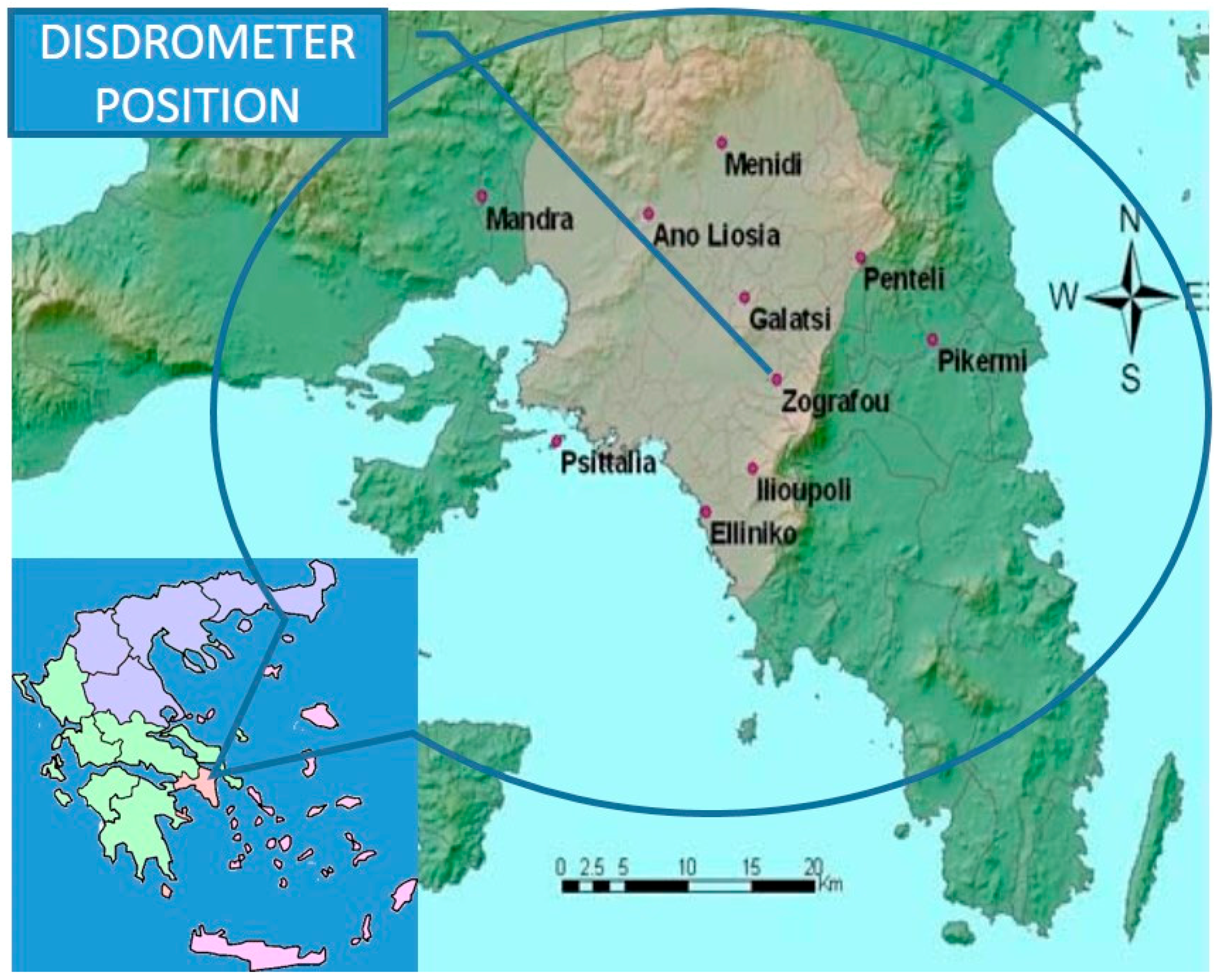
2. Study Area and Disdrometer Description
3. Methodology
3.1. Stratiform-Convective Rainfall Classification
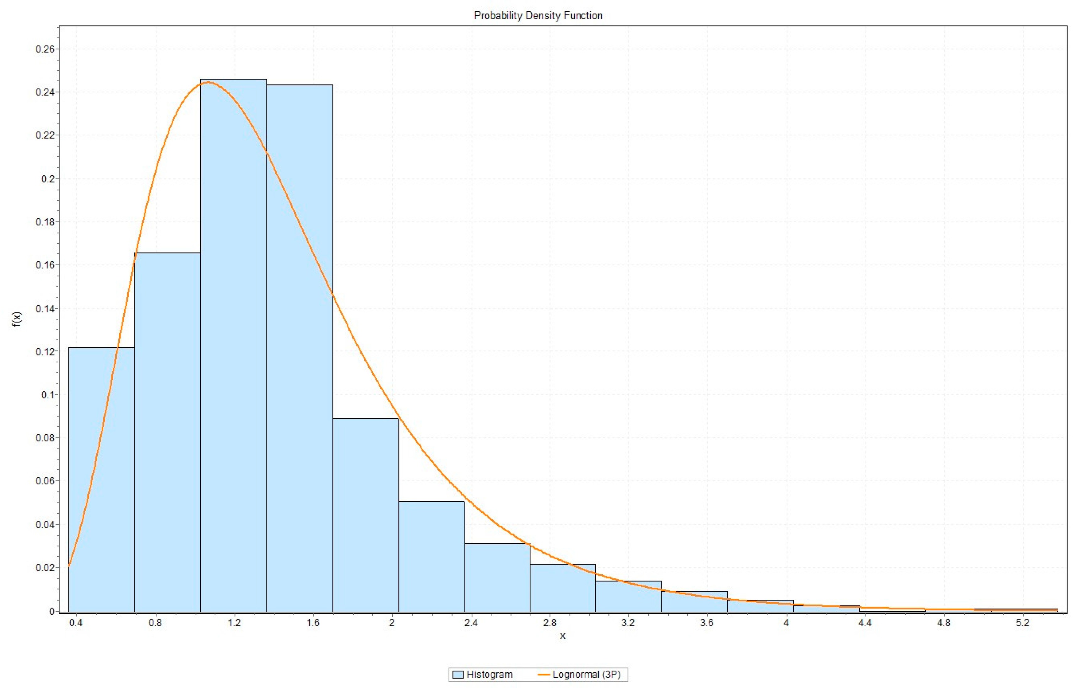
3.2. Statistical Distributions
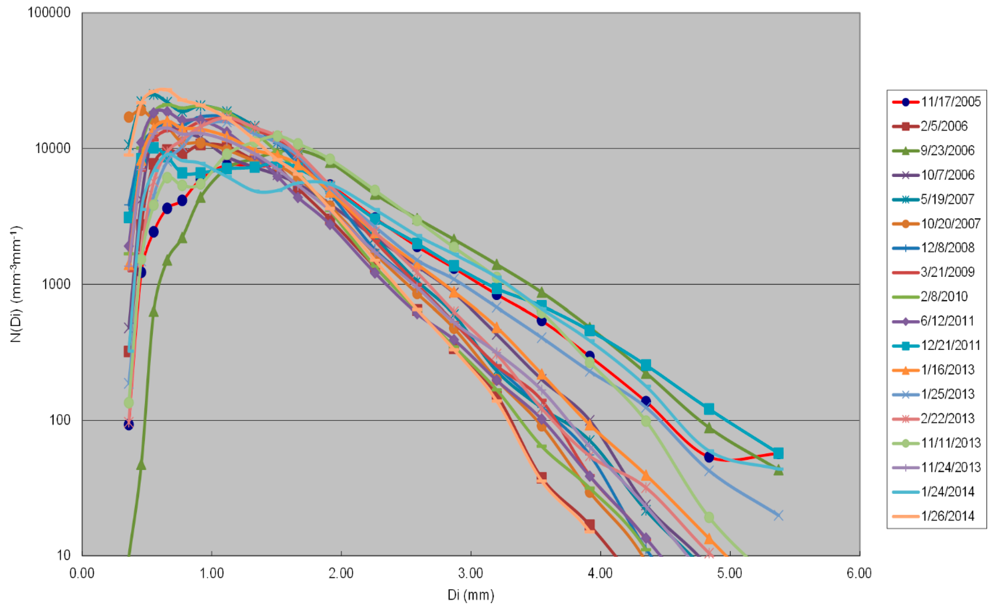
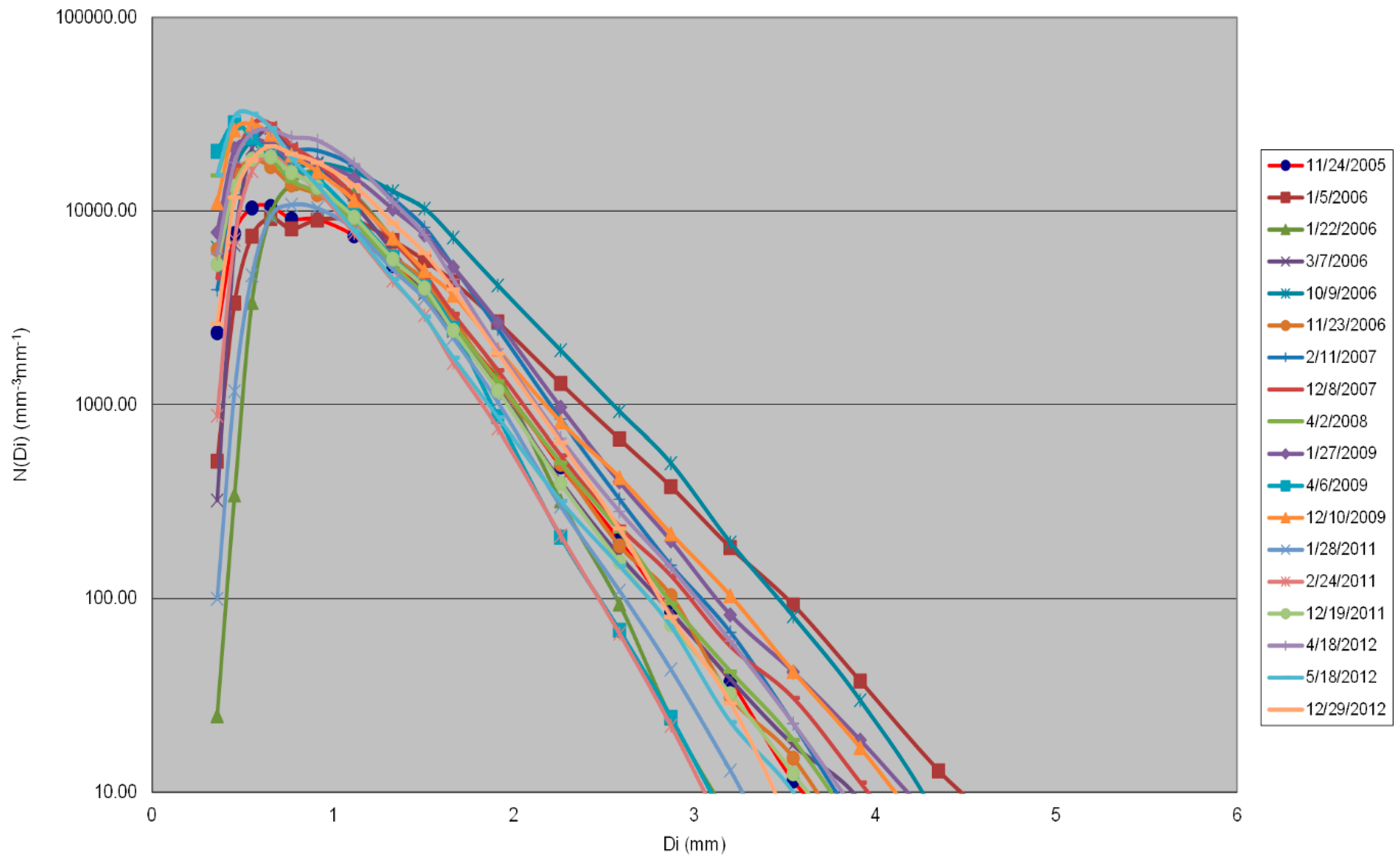
4. Results
5. Conclusions
Acknowledgments
Author Contributions
Conflicts of Interest
References
- Winder, P.; Paulson, K.S. The measurement of kinetic energy and rain intensity using an acoustic disdrometer. Meas. Sci. Technol. 2012, 23, 015801. [Google Scholar] [CrossRef]
- Kruger, A.; Krajewski, W.F. Two-Dimensional Video Disdrometer: A Description. J. Atmos. Oceanic Technol. 2002, 19, 602–617. [Google Scholar] [CrossRef]
- Schönhuber, M.; Lammer, G.; Randeu, W.L. The 2-D-Video-Distrometer. In Precipitation: Advances in Measurement, Estimation and Prediction; Springer: Berlin, German, 2008. [Google Scholar]
- Joss, J.; Waldvogel, A. Ein spektrograph fur niederschlagstrophen mit automatischer auswertung. Pure Appli. Geophys. 1967, 68, 240–246. [Google Scholar] [CrossRef]
- Ignaccolo, M.; De Michele, C. Phase space parameterization of rain: The inadequacy of gamma distribution. J. Appl. Meteor. Clim. 2014, 53, 548–562. [Google Scholar] [CrossRef]
- Adirosi, E.; Baldini, L.; Lombardo, F.; Russo, F.; Napolitano, F.; Volpi, E.; Tokay, A. Comparison of different fittings of drop spectra for rainfall retrievals. Adv. in W. Res. 2015, 83, 55–67. [Google Scholar] [CrossRef]
- Kottek, M.; Grieser, J.; Beck, C.; Rudolf, B.; Rubel, F. World map of the koppen-geiger climate classification updated. Met. Zeitschrift 2006, 15, 259–263. [Google Scholar] [CrossRef]
- Hellenic National Meteorological Service. Available online: http://www.hnms.gr/hnms/greek/index_html (accessed on 6 February 2016).
- Papathanasiou, C.; Makropoulos, C.; Baltas, E.; Mimikou, M. An innovative approach to floods and fire risk assessment and management: The flire project. In Procedings of the 8th International Conference of EWRA “Water Resources Management in an Interdisciplinary and Changing Context”, Porto, Portugal, 26–29 June 2013.
- Tokay, A.; Wolff, R.K.; Bashor, P.; Dursun, K.O. On the measurement errors of the joss-waldvogel disdrometer. In Procedings of the 31st International Conference on Radar Meteorology, Seattle, WA, USA, 6–12 August 2003.
- Tokay, A.; Kruger, A.; Krajewski, W.F. Comparison of drop size distribution measurements by impact and optical disdrometers. J. Appl. Meteorol. 2001, 40, 2083–2097. [Google Scholar] [CrossRef]
- Tokay, A.; Short, A.D. Evidence from tropical raindrop spectra of the origin of rain from stratiform versus convective clouds. J. App. Met. Clim. 1996, 35, 355–370. [Google Scholar] [CrossRef]
- Bringi, V.N.; Williams, C.R.; Thurai, M.; May, P.T. Using dual-polarized radar and dual-frequency profiler for dsd characterization: A case study from darwin, australia. J. Atm. Oc. Tech. 2009, 26, 2107–2122. [Google Scholar] [CrossRef]
- Caracciolo, C.; Prodi, F.; Battaglia, A.; Porcu, F. Analysis of the moments and parameters of a gamma dsd to infer precipitation properties: A convective stratiform discrimination algorithm. Atm. Res. 2006, 80, 165–186. [Google Scholar] [CrossRef]
- Ricciardulli, L.; Prashant, D.S. Local time and space scales of organized tropical deep convection. J. Clim. 2002, 15, 2775–2790. [Google Scholar] [CrossRef]
- Mathwave, T. Easyfit, 5.6 Professional. Available online: http://www.mathwave.com/company.html (accessed on 6 February 2016).
- Marshall, J.S.; Palmer, W.M. The distribution of raindrops with size. J. Meteor. 1948, 5, 165–166. [Google Scholar] [CrossRef]
- Ulbrich, W.C. Natural variations in the analytical form of the raindrop size distribution. J. Clim. Appl. Meteorol. 1983, 22, 1764–1775. [Google Scholar] [CrossRef]
- Feingold, G.; Levin, Z. The lognormal fit to raindrop spectra from convective clouds in israel. J. Clim. Appl. Meteorol. 1986, 25, 1346–1363. [Google Scholar] [CrossRef]
- Kliche, V.D.; Smith, L.P.; Johnson, W.R. L-moment estimators as applied to gamma drop size distributions. J. Appl. Meteorol. Clim. 2008, 47, 3117–3130. [Google Scholar] [CrossRef]
- Cao, Q.; Zhang, G. Errors in estimating raindrop size distribution parameters employing disdrometer and simulated raindrop spectra. J. Appl. Meteorol. Clim. 2009, 48, 406–425. [Google Scholar] [CrossRef]


| Stratiform | Convective | ||||||
|---|---|---|---|---|---|---|---|
| No | Rainfall Event | TD(min) | RD(mm) | No | Rainfall Event | TD(min) | RD(mm) |
| 1 | 24-11-05 | 536 | 17.98 | 1 | 17-11-05 | 162 | 12.05 |
| 2 | 05-01-06 | 536 | 40.04 | 2 | 05-02-06 | 136 | 46.92 |
| 3 | 22-01-06 | 540 | 18.78 | 3 | 23-09-06 | 116 | 13.22 |
| 4 | 07-03-06 | 440 | 15.61 | 4 | 07-10-06 | 144 | 15.84 |
| 5 | 09-10-06 | 540 | 58.63 | 5 | 19-05-07 | 158 | 14.67 |
| 6 | 23-11-06 | 408 | 14.94 | 6 | 20-10-07 | 112 | 13.57 |
| 7 | 11-02-07 | 622 | 40.82 | 7 | 18-12-08 | 144 | 17.94 |
| 8 | 08-12-07 | 640 | 29.7 | 8 | 21-03-09 | 142 | 13.59 |
| 9 | 02-04-08 | 626 | 23.04 | 9 | 08-02-10 | 164 | 13.45 |
| 10 | 27-01-09 | 376 | 24.57 | 10 | 12-06-11 | 148 | 41.12 |
| 11 | 06-04-09 | 428 | 12.25 | 11 | 21-12-11 | 176 | 21.64 |
| 12 | 10-12-09 | 490 | 26.66 | 12 | 16-01-13 | 164 | 33.64 |
| 13 | 28-01-11 | 496 | 13.31 | 13 | 25-01-13 | 96 | 13.71 |
| 14 | 24-02-11 | 528 | 11.85 | 14 | 11-11-13 | 58 | 16.64 |
| 15 | 19-12-11 | 630 | 21.33 | 15 | 24-11-13 | 140 | 14.87 |
| 16 | 18-04-12 | 376 | 21.69 | 16 | 24-01-14 | 148 | 24.81 |
| 17 | 18-05-12 | 590 | 16.9 | 17 | 26-01-14 | 140 | 12.68 |
| 18 | 29-12-12 | 432 | 21.09 | 18 | 22-02-13 | 274 | 63.15 |
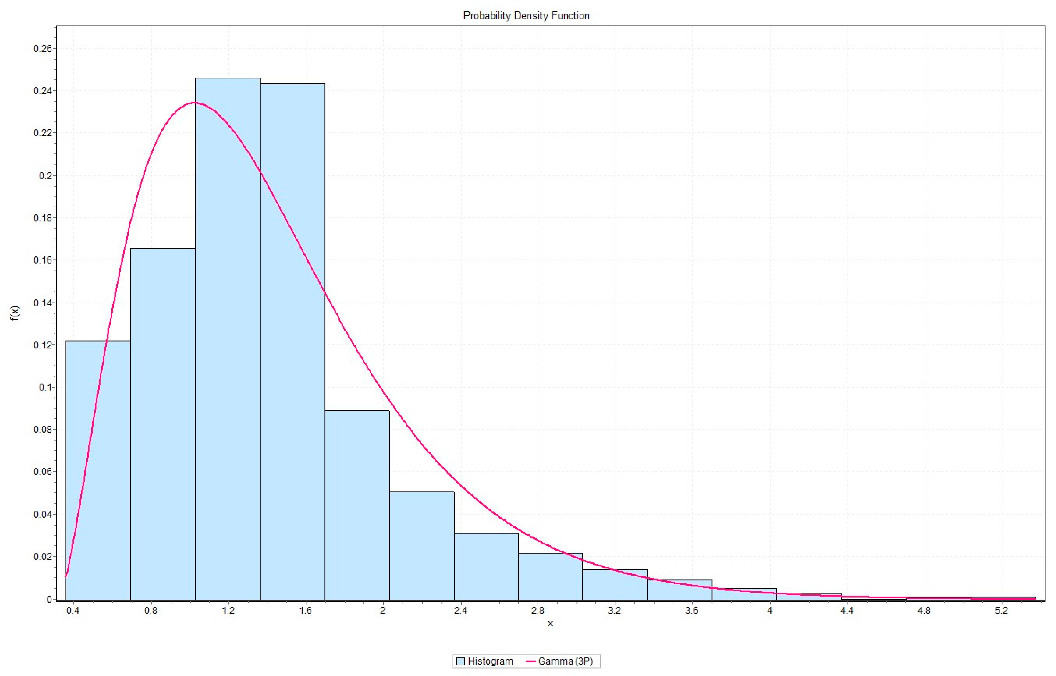
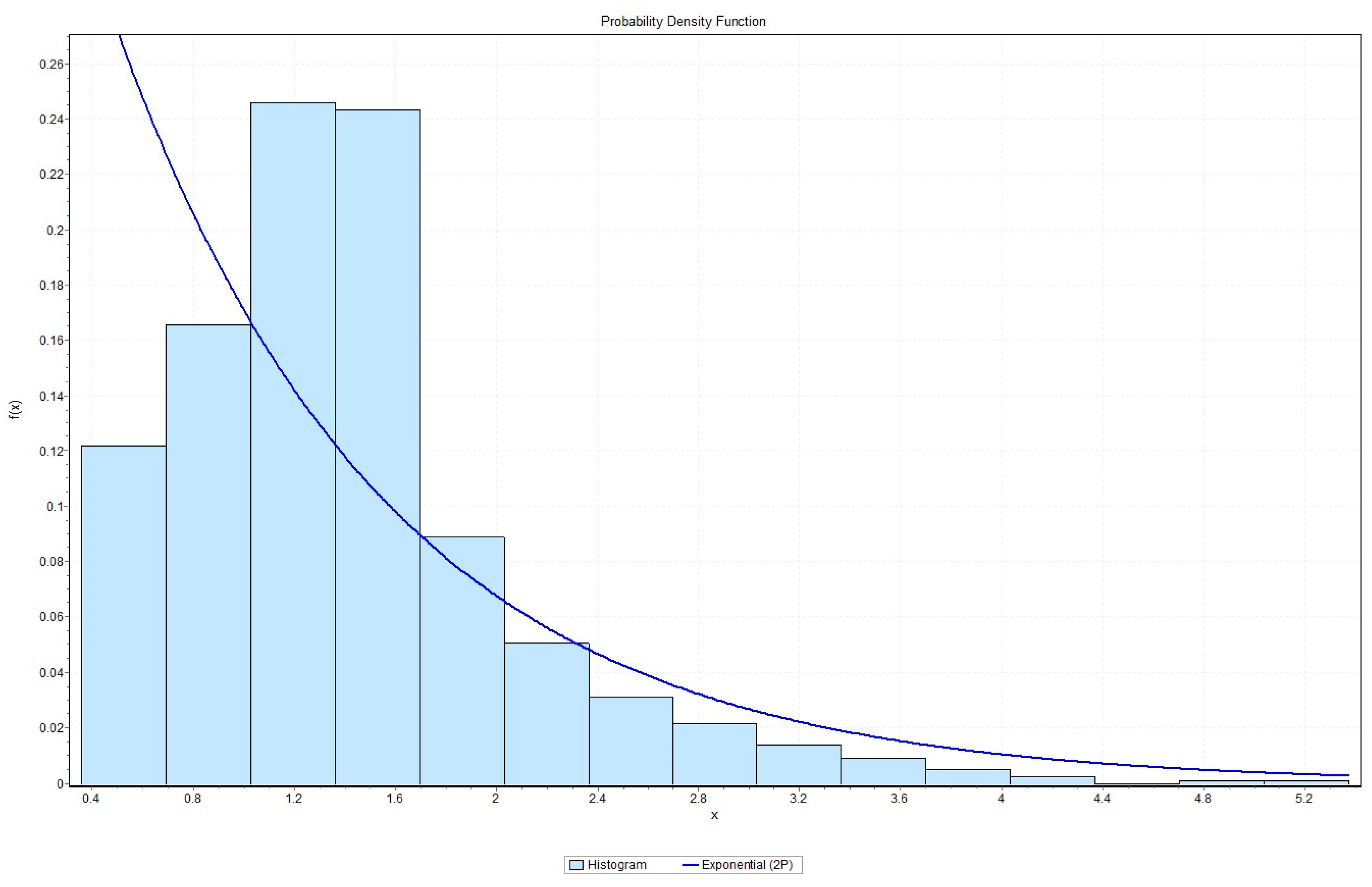
| Fitting Results | Convective Event of 17-11-05 | |
|---|---|---|
| Distribution | Parameters | |
| 1 | Exponential (1P) | λ = 0.7468 |
| 2 | Exponential (2P) | λ = 0.97022 γ = 0.30835 |
| 3 | Gamma (2P) | α = 4.2996 β = 0.31143 |
| 4 | Gamma (3P) | α = 2.7315 β = 0.38971 γ = 0.27455 |
| 5 | Lognormal (2P) | σ = 0.47132 μ = 0.18308 |
| 6 | Lognormal (3P) | σ = 0.44221 μ = 0.24633 γ = −0.07061 |
| Event Date | Exponential (1P) | Exponential (2P) | Gamma (2P) | Gamma (3P) | Lognormal (2P) | Lognormal (3P) |
|---|---|---|---|---|---|---|
| 24/11/2005 | 6 | 5 | 4 | 1 | 3 | 2 |
| 5/1/2006 | 6 | 5 | 4 | 1 | 3 | 2 |
| 22/1/2006 | 6 | 5 | 4 | 2 | 3 | 1 |
| 7/3/2006 | 6 | 5 | 4 | 2 | 3 | 1 |
| 9/10/2006 | 6 | 5 | 3 | 1 | 4 | 2 |
| 23/11/2006 | 6 | 5 | 3 | 2 | 4 | 1 |
| 11/2/2007 | 6 | 5 | 4 | 1 | 3 | 2 |
| 8/12/2007 | 6 | 5 | 4 | 2 | 3 | 1 |
| 2/4/2008 | 6 | 2 | 3 | 5 | 4 | 1 |
| 27/1/2009 | 6 | 5 | 3 | 2 | 4 | 1 |
| 6/4/2009 | 6 | 4 | 2 | 5 | 3 | 1 |
| 10/12/2009 | 6 | 2 | 4 | 5 | 3 | 1 |
| 28/1/2011 | 6 | 5 | 4 | 2 | 3 | 1 |
| 24/2/2011 | 6 | 5 | 4 | 2 | 3 | 1 |
| 19/12/2011 | 6 | 5 | 4 | 2 | 3 | 1 |
| 18/4/2012 | 6 | 5 | 4 | 1 | 3 | 2 |
| 18/5/2012 | 6 | 4 | 3 | 5 | 2 | 1 |
| 29/12/2012 | 6 | 5 | 4 | 2 | 3 | 1 |
| Best fit | 0 | 0 | 0 | 5 | 0 | 13 |
| Percentage | 0% | 0% | 0% | 28% | 0% | 72% |
| Event Date | Exponential (1P) | Exponential (2P) | Gamma (2P) | Gamma (3P) | Lognormal (2P) | Lognormal (3P) |
|---|---|---|---|---|---|---|
| 11/17/2005 | 6 | 5 | 1 | 2 | 4 | 3 |
| 2/5/2006 | 6 | 5 | 4 | 1 | 2 | 3 |
| 9/23/2006 | 6 | 5 | 4 | 3 | 1 | 2 |
| 10/7/2006 | 6 | 5 | 3 | 2 | 4 | 1 |
| 5/19/2007 | 6 | 3 | 2 | 5 | 4 | 1 |
| 10/20/2007 | 6 | 3 | 4 | 5 | 2 | 1 |
| 12/8/2008 | 6 | 5 | 1 | 2 | 3 | 4 |
| 3/21/2009 | 6 | 5 | 1 | 2 | 3 | 4 |
| 2/8/2010 | 6 | 5 | 4 | 1 | 3 | 2 |
| 6/12/2011 | 6 | 5 | 4 | 2 | 3 | 1 |
| 12/21/2011 | 6 | 2 | 1 | 5 | 3 | 4 |
| 1/16/2013 | 6 | 5 | 3 | 2 | 4 | 1 |
| 1/25/2013 | 6 | 5 | 1 | 2 | 3 | 4 |
| 2/22/2013 | 6 | 5 | 1 | 2 | 3 | 4 |
| 11/11/2013 | 6 | 5 | 1 | 3 | 4 | 2 |
| 11/24/2013 | 6 | 5 | 4 | 1 | 3 | 2 |
| 1/24/2014 | 6 | 5 | 4 | 2 | 3 | 1 |
| 1/26/2014 | 6 | 5 | 4 | 2 | 3 | 1 |
| Best fit | 0 | 0 | 7 | 3 | 1 | 7 |
| Percentage | 0% | 0% | 39% | 17% | 6% | 39% |
© 2016 by the authors; licensee MDPI, Basel, Switzerland. This article is an open access article distributed under the terms and conditions of the Creative Commons by Attribution (CC-BY) license (http://creativecommons.org/licenses/by/4.0/).
Share and Cite
Baltas, E.; Panagos, D.; Mimikou, M. Statistical Analysis of the Raindrop Size Distribution Using Disdrometer Data. Hydrology 2016, 3, 9. https://doi.org/10.3390/hydrology3010009
Baltas E, Panagos D, Mimikou M. Statistical Analysis of the Raindrop Size Distribution Using Disdrometer Data. Hydrology. 2016; 3(1):9. https://doi.org/10.3390/hydrology3010009
Chicago/Turabian StyleBaltas, Evangelos, Dimitris Panagos, and Maria Mimikou. 2016. "Statistical Analysis of the Raindrop Size Distribution Using Disdrometer Data" Hydrology 3, no. 1: 9. https://doi.org/10.3390/hydrology3010009