Article

Results from the First Phase of the Seafloor Backscatter Processing Software Inter-Comparison Project

1
NOAA Office of Ocean Exploration and Research, Silver Spring, MD 20910, USA
2
Center for Coastal and Ocean Mapping, University of New Hampshire, Durham, NH 03824, USA
3
National Institute of Water and Atmospheric Research (NIWA), Greta Point, Wellington 6021, New Zealand
4
Federal Public Service Economy of Belgium (FPSE), 1210 Brussels, Belgium
5
Service Hydrographique et Océanographique de la Marine (SHOM), 29200 Brest, France
6
Geological Survey of Norway (NGU), 7491 Trondheim, Norway
7
QPS B.V. Fredericton, Fredericton, NB E3B 1P9, Canada
8
Service Acoustique Sous-marine et Traitement de l’Information, IFREMER, 29280 Plouzane, France
9
Teledyne CARIS, Fredericton, NB E3B 2L4, Canada
10
Centre for Marine Science and Technology, Curtin University, Perth 2605, Australia
*
Author to whom correspondence should be addressed.
Geosciences 2019, 9(12), 516; https://doi.org/10.3390/geosciences9120516
Submission received: 15 November 2019 / Revised: 9 December 2019 / Accepted: 11 December 2019 / Published: 16 December 2019
(This article belongs to the Section Geophysics)

Abstract

:
Seafloor backscatter mosaics are now routinely produced from multibeam echosounder data and used in a wide range of marine applications. However, large differences (>5 dB) can often be observed between the mosaics produced by different software packages processing the same dataset. Without transparency of the processing pipeline and the lack of consistency between software packages raises concerns about the validity of the final results. To recognize the source(s) of inconsistency between software, it is necessary to understand at which stage(s) of the data processing chain the differences become substantial. To this end, willing commercial and academic software developers were invited to generate intermediate processed backscatter results from a common dataset, for cross-comparison. The first phase of the study requested intermediate processed results consisting of two stages of the processing sequence: the one-value-per-beam level obtained after reading the raw data and the level obtained after radiometric corrections but before compensation of the angular dependence. Both of these intermediate results showed large differences between software solutions. This study explores the possible reasons for these differences and highlights the need for collaborative efforts between software developers and their users to improve the consistency and transparency of the backscatter data processing sequence.

1. Introduction

Commercial Multibeam echosounders (MBES) were designed in the 1970’s [1] for the purpose of bathymetry data acquisition, but it is only in the past two decades that software packages generally became available to process seafloor backscatter data (henceforth, backscatter). The earliest software packages were developed and privately used by academics [2,3]. As backscatter started proving important in seafloor characterization studies [4,5,6,7], the user base expanded, and several commercial, proprietary software packages became available. Today, backscatter is collected by a broad range of users for a variety of applications, including scientists and resource managers to assess and quantify seafloor resources (sediment, geology, habitats, etc.), by hydrographic and military agencies to determine seafloor type, and by coastal zone managers for infrastructure planning. Most of these end-users rely on commercial software for data processing [8]. Due to their commercial nature, these software packages are often closed source, and very limited information is available about their proprietary data processing routines and algorithms.
Processing backscatter data involves applying various and complex environmental and sensor-specific corrections to the raw level recorded by the system [9]. Those corrections have been well studied [6,7,9,10], but neither the details of each correction nor the order in which they are applied has ever been standardized [9,10,11]. This lack of standards for data processing and metadata, combined with the need for commercial software manufacturers to protect their intellectual property, resulted in software being developed mostly independently. Recent comparisons of the backscatter products obtained from processing the same datasets with different software highlighted differences in the results [8,12,13,14]. The approach adopted during these comparisons included comparing the backscatter end-results in the form of mosaics as obtained from various software packages. Having recognized that different software likely process backscatter differently, the challenge remains for the end-users to assess which, if any, of the processing methodology is most accurate. This challenge is further compounded by the lack of standards for backscatter data acquisition [10,15]. The uncertainty in backscatter results due to the hardware and environment have only recently begun to be recognized [15,16], and uncertainty standards still need to be developed in the manner that they were developed for multibeam bathymetry data over a decade ago [17]. With the goal of improving consistency among backscatter data acquisition and processing methodologies, the Backscatter Working Group (BSWG) was established in 2013 under the auspices of the GeoHab (Marine Geological and Biological Habitat Mapping) association. The BSWG compiled its guidelines in a report published in 2015 [11]. Among other recommendations, the BSWG encouraged comparative tests of processing software packages using common data sets [10]. As an outcome of this recommendation, the Backscatter Software Inter-Comparison Project (BSIP) was launched during the GeoHab 2019 conference.
The long-term objective of the Backscatter Inter-comparison Project is to understand the reasons for the differences between the end-results obtained from a common dataset by various backscatter processing tools. The results in this paper represent the first phase of this project. Since comparing the end-results of the processing solutions does not allow for understanding the root causes of the discrepancies, the developers of commonly-used software were invited to provide a set of intermediate stages from the processing of a common dataset. This approach allows a comparison of intermediate corrections without requiring software developers to disclose the details of their proprietary algorithms.
A recent survey of backscatter end-users [8] identified the most-commonly used backscatter data processing software packages to date: Hydrographic Information Processing System and Sonar Information Processing System (HIPS and SIPS) by Teledyne CARIS, the Fledermaus Geocoder Toolbox (FMGT) by QPS, Geocoder by the University of New Hampshire (UNH), Hypack by the Xylem, MB-System by the Monterey Bay Aquarium Research Institute, and Sonarscope by IFREMER. The developers of FMGT [18], HIPS and SIPS [19], SonarScope [20], and the MB-Process (a data processing research tool by Curtin University) agreed to participate in this study. This paper describes the results of the first phase of the project and the lessons learned.

2. Materials and Methods

2.1. Selection of Test Backscatter Data

Five datasets were selected for this study (Table 1), representing a range of shallow- and deep-water MBES: Kongsberg EM 2040, EM 3002, EM 710, EM 302, and Teledyne Reson SeaBat 7125. These datasets do not represent an exhaustive list of commercially available MBES but were opportunistically chosen because data from these surveys were publicly available. The test datasets were collected by different agencies (Table 1). The list of individual data files used during this study is provided as Appendix A (Table A1). The common datasets used in this project are publicly available at https://bswg.github.io/bsip/.

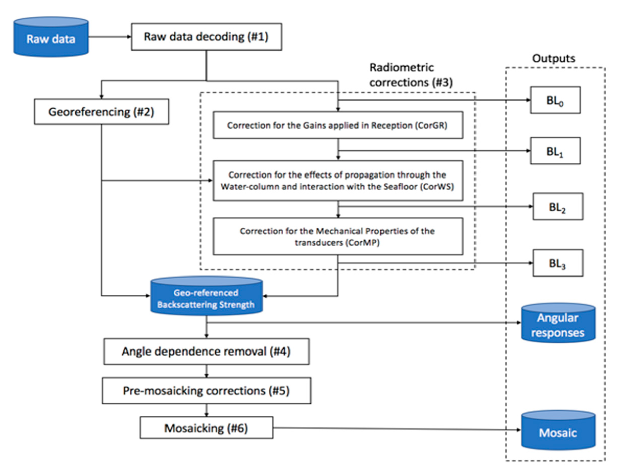
2.2. Selection of Intermediate Processed Backscatter Levels

A template backscatter data processing pipeline and nomenclature were recently proposed for adoption to assist standardizing backscatter data processing [9]. In this theoretical pipeline, the various stages of radiometric and geometric corrections are chronologically ordered, and the intermediate backscatter levels obtained between each stage are named (BL0 through to BL4), providing a sequence of intermediate results (Figure 1). However, since each software package applies these corrections in different orders, most of these specific outputs cannot be produced without significantly modifying the data processing code. For the current study, after discussion and agreement with software developers, it was concluded that a phased approach would be most effective. In this first phase, only the intermediate levels that can be provided without significantly altering the code (i.e., BL0 and BL3) were considered.

2.2.1. BL0: The Backscatter Level as Read in The Raw Files

The first stage of backscatter processing consists of reading the raw backscatter data recorded in the MBES raw data files. For both Kongsberg and Teledyne Reson systems, the raw data format organizes the collected information into several types of data units, known as datagrams, and the structure of each datagram type is described in format specifications made publicly available by the manufacturers [21,22]. Not only are backscatter data typically available in different datagrams, but the formats, the intermediate calculations applied, and the output resolution may have changed over the years. For example, in Kongsberg systems, the backscatter data are available in both the “one-value-per-beam” and “several-samples-per-beam” formats in two different datagrams (“Depth” datagram for the former and “Seabed Image” datagram for the later). In November 2005, the “Depth” datagram was superseded by the “XYZ 88” datagram, and the “Seabed Image” datagram was superseded by the “Seabed Image 89” datagram, with both newer datagrams upgrading the data resolution from 0.5 dB to 0.1 dB [21]. Although Kongsberg released KMALL format in 2017 [23], this format has not been adopted widely by the processing software packages and was not considered during this study. For the Reson system, datagrams with multiple samples per beam data are referred to as “snippets”. With the aim of using the same raw data, software developers were requested to start the processing with the Seabed Image / Snippets data as the basis to calculate BL0.

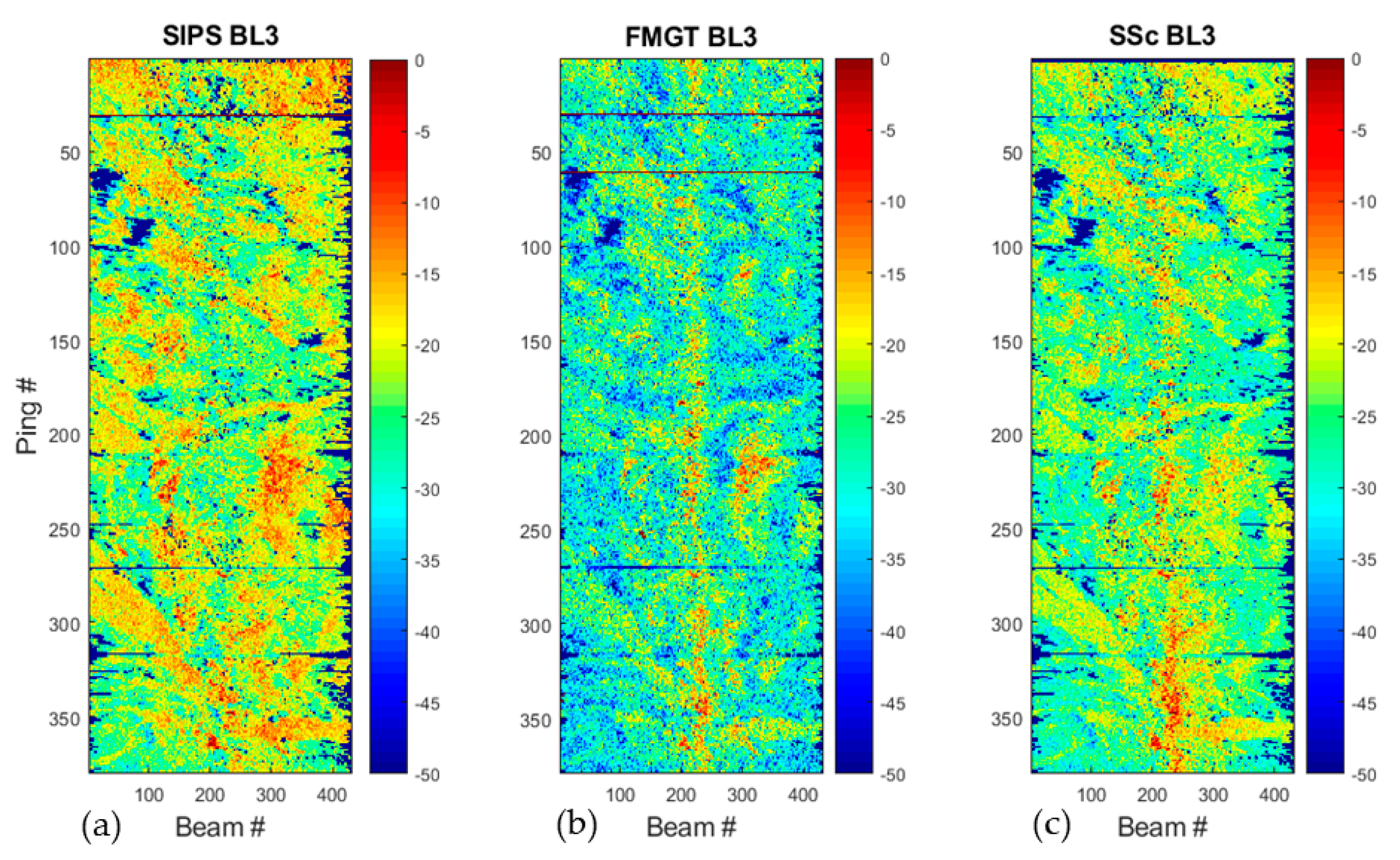
2.2.2. BL3: The Backscatter Level After Radiometric Corrections but Before Compensation for Angular Dependence

Typically, several radiometric corrections are applied to the raw data (BL0) after they are extracted from the file. Schimel et al. [9] suggest the following three classifications: (i) Corrections for Gains applied during Reception (CorGR), (ii) Corrections for propagation through Water column and interaction with Seafloor and (CorWS) and (iii) Corrections for Mechanical Properties of the transducer (CorMP). This is not the approach that has been historically taken in different software implementations; some software may apply all corrections in bulk, others may combine several, or apply only partial corrections, or apply corrections in different orders. Therefore, this study could only request the levels before and after all radiometric corrections (BL0 and BL3, see Figure 2). BL3, the backscatter level corrected for radiometric corrections, as a function of the incident angle, is the “angular response curve”, that is one of the two backscatter outputs commonly produced. Further corrections would need to be applied to BL3 to obtain a backscatter mosaic, including the flattening of the backscatter angular dependence.

2.3. Data Processing by Software Developers

Software developers provided the results as an ASCII text file in the format requested (Table 2). One of the software packages already had some variations of the ASCII export built into their processing routine, while for others, the ASCII export was developed as a result of this request.
Software developers were given the option to include additional columns as desired. The details of the data processing, as implemented by software developers for this project, are outlined in the following sections.

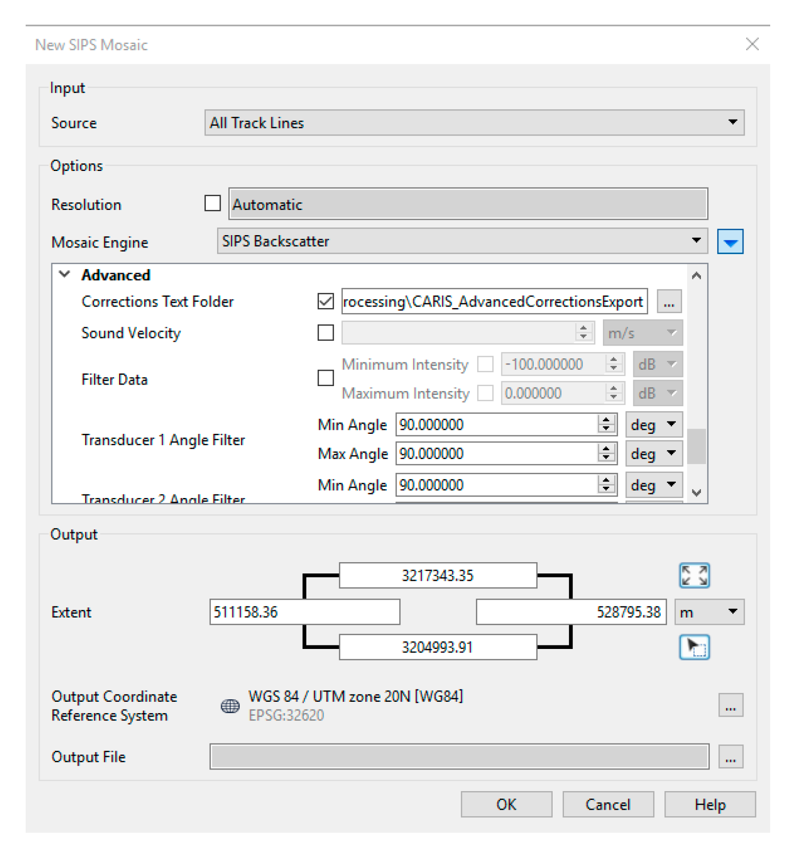
2.3.1. CARIS SIPS Backscatter Processing Workflow

The backscatter processing implementation in CARIS SIPS is a continuation of its bathymetric processing workflow and is aimed towards creating a backscatter mosaic. SIPS supports data sources from Reson and Kongsberg systems in their three record modes: Side scan (only applicable to Reson systems), beam average intensities, and snippets. Two separate backscatter processing engines are available within SIPS: Geocoder and SIPS backscatter processing engine. As the existing SIPS workflow did not allow end-users to extract BL0 and BL3, these data were extracted by the SIPS software developers themselves. The following corrections and settings were selected: Processing Engine: SIPS; Source Data Type: Time series; Slant Range Correction, Beam Pattern Correction; Angular Variation Gains, Adaptive; AVG size filter, 200 samples. As of the release of the CARIS SIPS 11.1.3 (released March 2019), end-users have the ability to export the intermediate processing stages utilized in SIPS processing engine accessed through ‘Advanced Settings’ and by designating a ‘Corrections Text Folder’ where an ASCII file is stored that contains results of intermediate processing stages. (Figure 2).

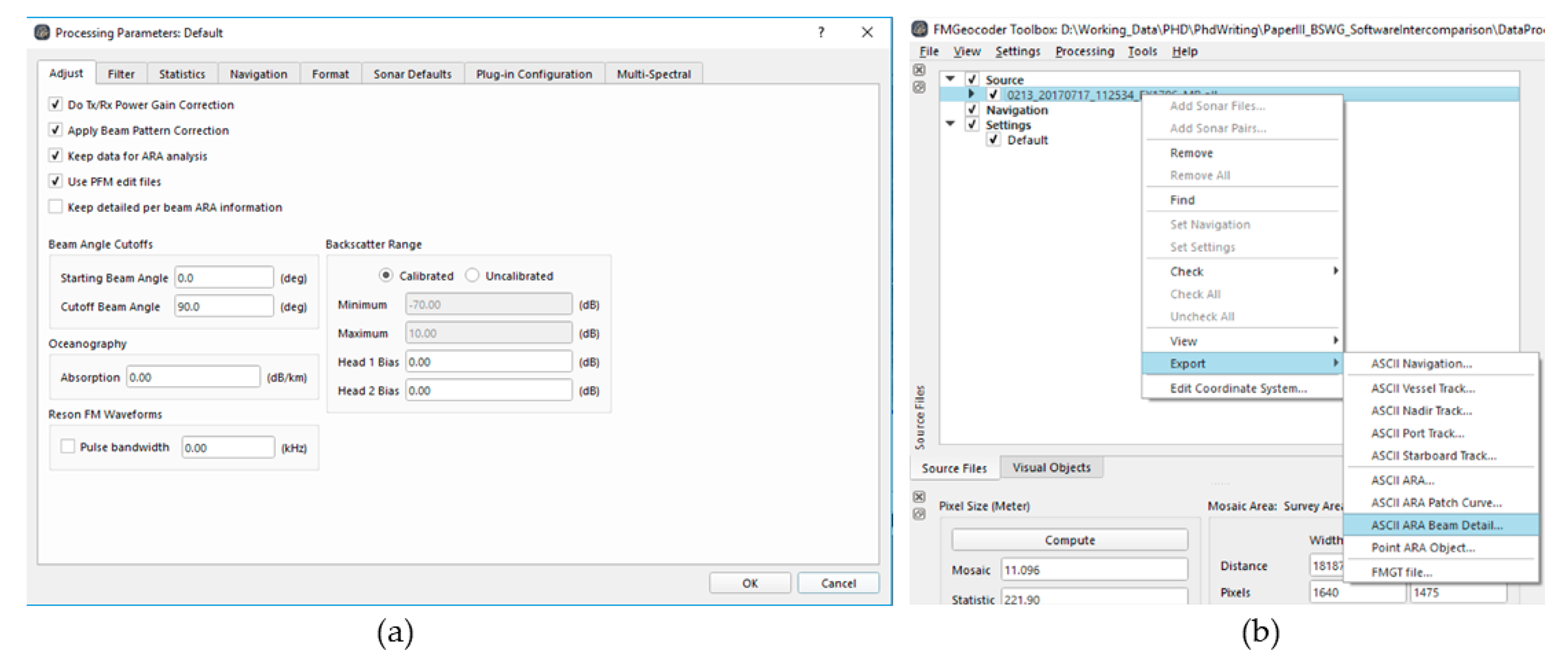
2.3.2. FMGT Backscatter Processing Workflow

The backscatter data processing in the QPS software suite is implemented in a separate toolbox: Fledermaus Geocoder Toolbox (FMGT). A notable factor in this implementation is that all the survey parameters are read directly from the survey line files. The processing parameters used included “Tx/Rx Power Gain Correction”, “Apply Beam Pattern Correction”, and “Keep data for ARA (Angle Range analysis)”. Backscatter Range was selected based on the minimum and maximum value of backscatter from “calibrated” backscatter with beam angle cut off between 0° and 90°. Export of BL0 and BL3 data are available through export ‘ASCII ARA beam detail’ (Figure 3).

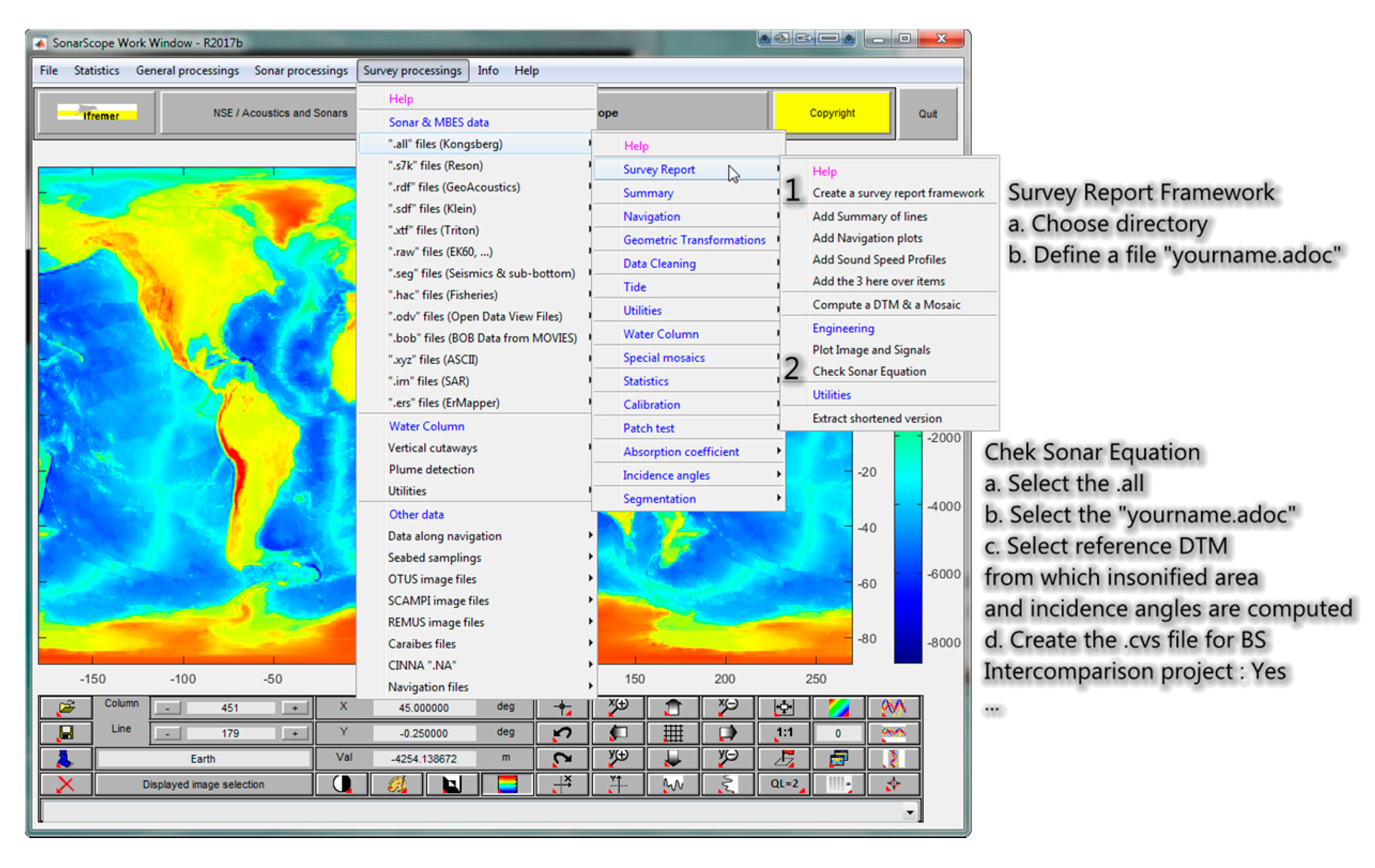
2.3.3. SonarScope Data Processing Workflow

SonarScope is a research tool developed by the department of Underwater Acoustics at IFREMER. SonarScope is available for free under an academic non-commercial use license. This tool is developed in Matlab as a laboratory tool aimed at research and development, rather than production. SonarScope can handle a variety of MBES formats. SonarScope implemented a new backscatter data processing methodology concurrently with this study. A detailed analysis of various processing stages based on the sonar equation [7] is provided in this updated workflow and exported as an HTML summary file with graphical displays of the various corrections. An ASCII output file is also produced that contains several fields describing the corrections (Figure 4).

2.3.4. MB Process Data Processing and SONAR2MAT Data Conversion

MB Process is a proprietary backscatter data processing tool coded in Matlab and developed and used by Curtin University Centre for Marine Science and Technology (CMST) and Geoscience Australia (GA) researchers to process Kongsberg (.all) files and Reson MBES (files saved as XTF) [24]. CMST-GA MB Process is available to download for free from https://cmst.curtin.edu.au/products/multibeam-software/ (last accessed September 2019). As this study used Reson (.s7k) files, the converter SONAR2MAT [25] was used to convert the (.s7k) data first to MATLAB (.mat) data files. SONAR2MAT converter supports a variety of MBES data formats and is available to download for free from https://cmst.curtin.edu.au/products/sonar2mat-software/ (last accessed Sept 2019). The script was used to calculate the mean for each beam (i.e., BL0) from the converted snippets data packet (7028) using the samples that fall within +/− 5 dB around the bottom detect echo level. The corrections applied followed Parnum and Gavrilov [26], and required other converted data packets including settings (7000), bathymetry (7027), and beam geometry (7004), to produce BL3 data. Data were then exported in to the ASCII format specified in Table 2 except for beam depth.

3. Results

The ASCII files obtained for each software differed in both format and contents. A summary of the contents of the ASCII files is provided in Appendix B (Table A2). The availability of the results on ping/beam basis made it convenient to compare data from each software. Data inter-comparison was conducted based on the ping/beam number, BL0, BL3, and incidence angle.

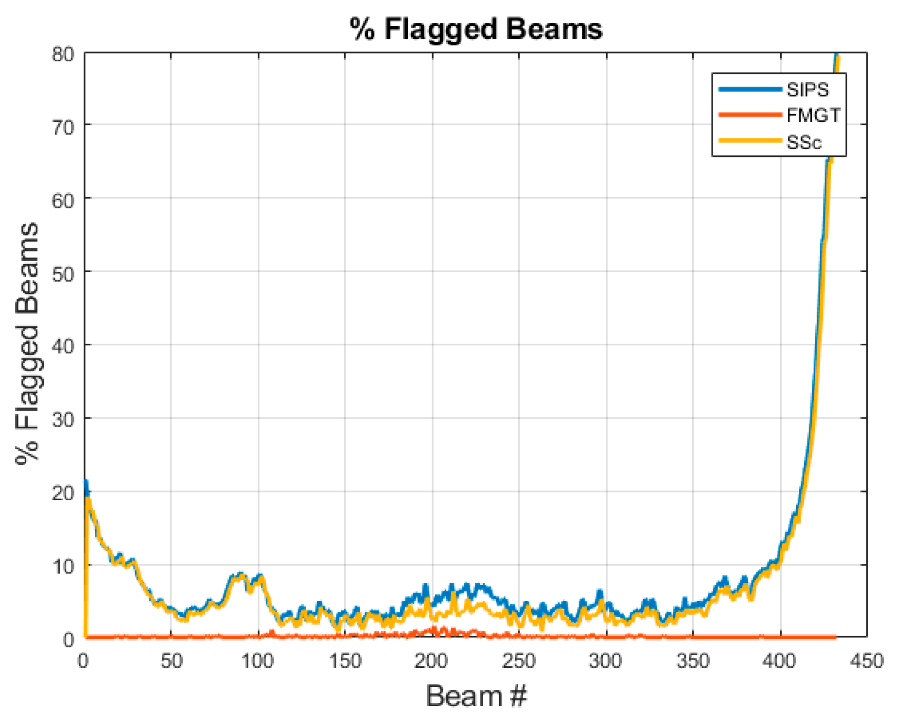
3.1. Flagged Invalid Beams

The number of beams flagged as “invalid” by each software was different (Figure 5). For the Kongsberg EM 302 data, FMGT showed almost no flagged beams while both SIPS and SonarScope showed a large number of beams flagged. These differences were found to be related to each software’s different choice of dealing with soundings with invalid bottom detection. Kongsberg’s “XYZ 88” datagram provides information about ‘detection information’ that specifies among other things whether the beam had a valid bottom detection or not. The beams with invalid bottom detections, however, can be assigned interpolated backscatter to provide continuous backscatter across all beams (see note 4 p.44 [21]). FMGT has implemented the strategy to use the beams with invalid bottom detection, while SIPS and SonarScope utilize only the beams that have a valid bottom detection information available. For the purposes of comparison, only the beams that were considered valid by all software packages were used.

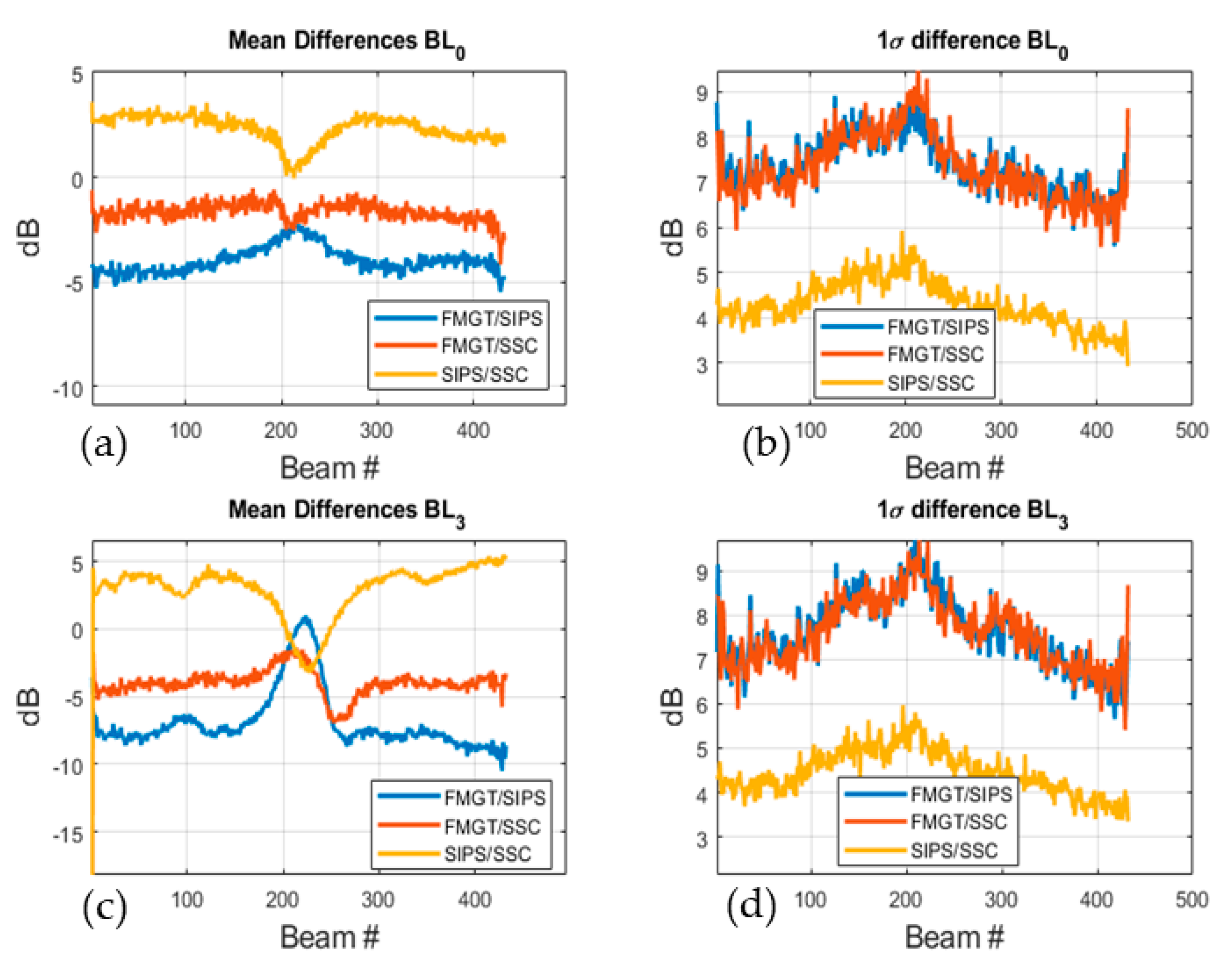
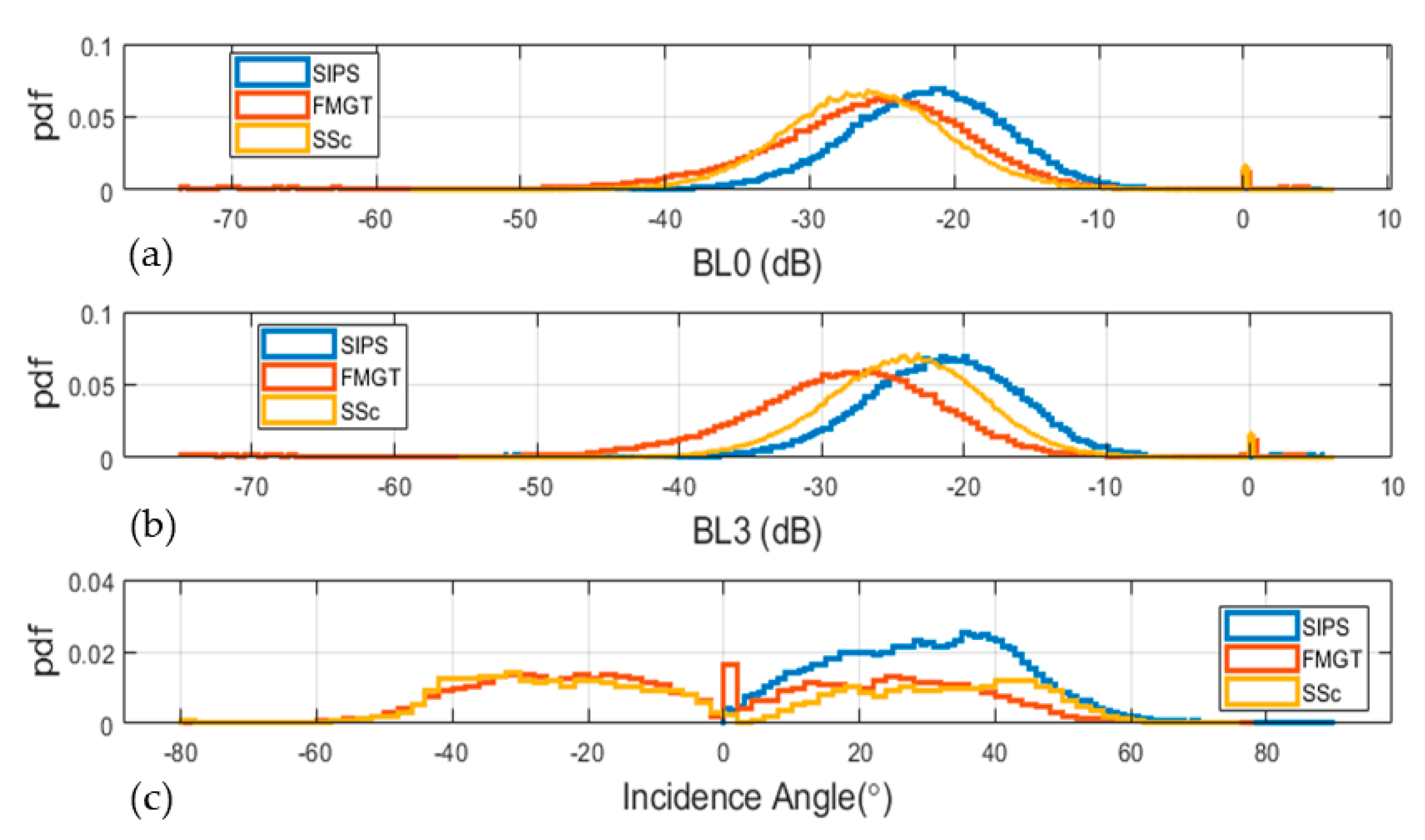
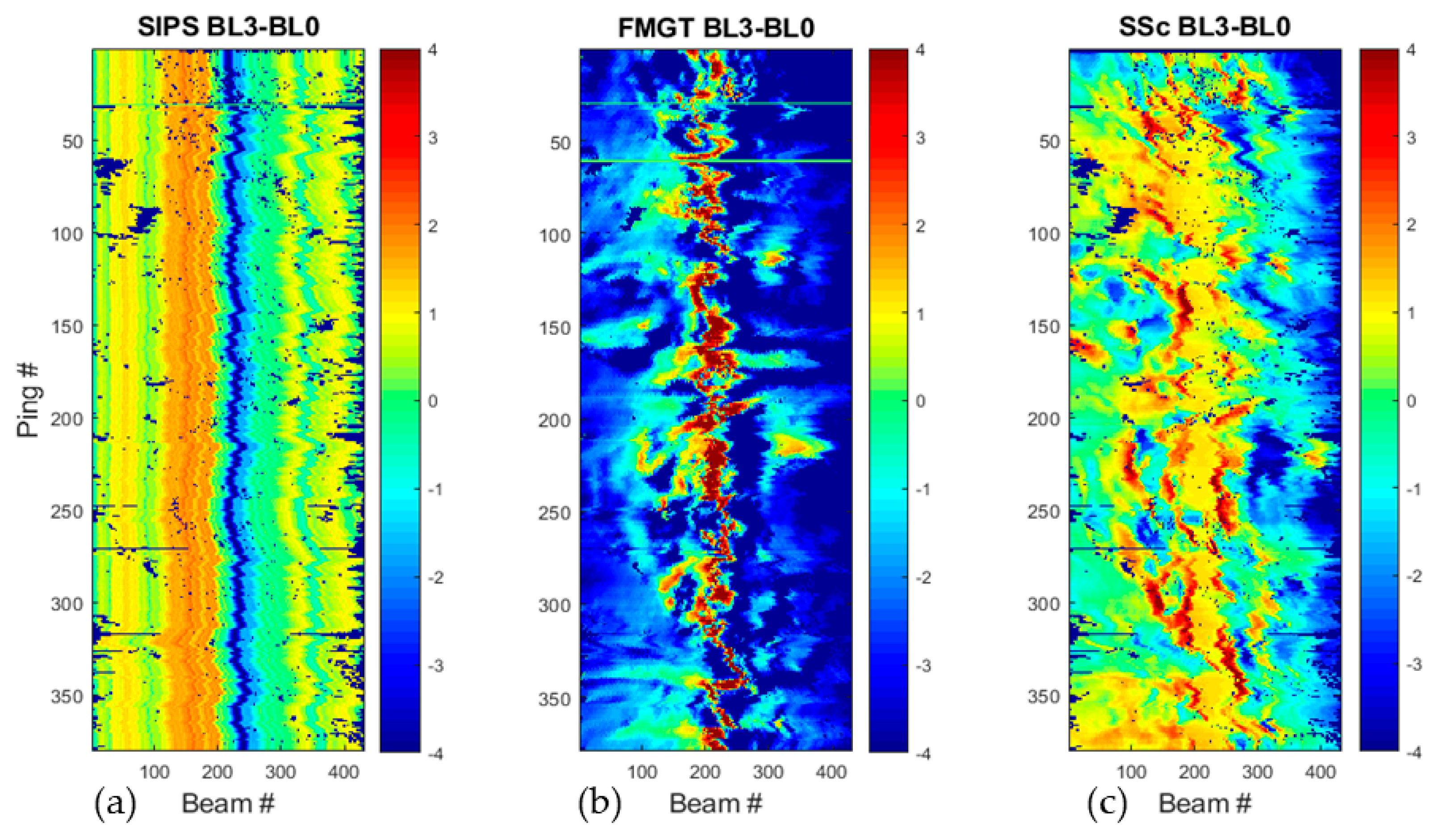
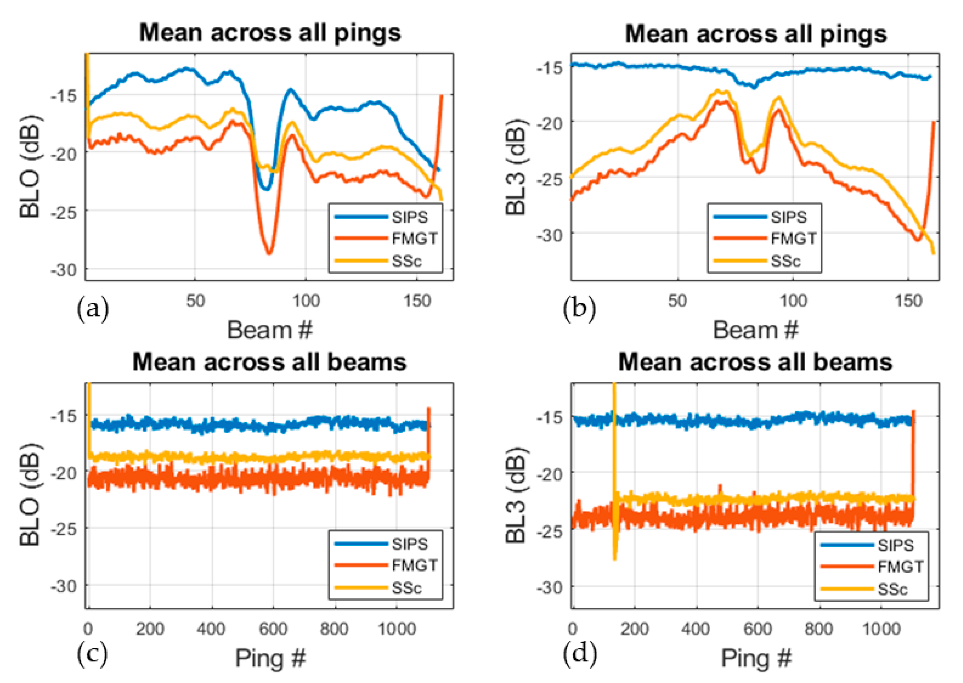
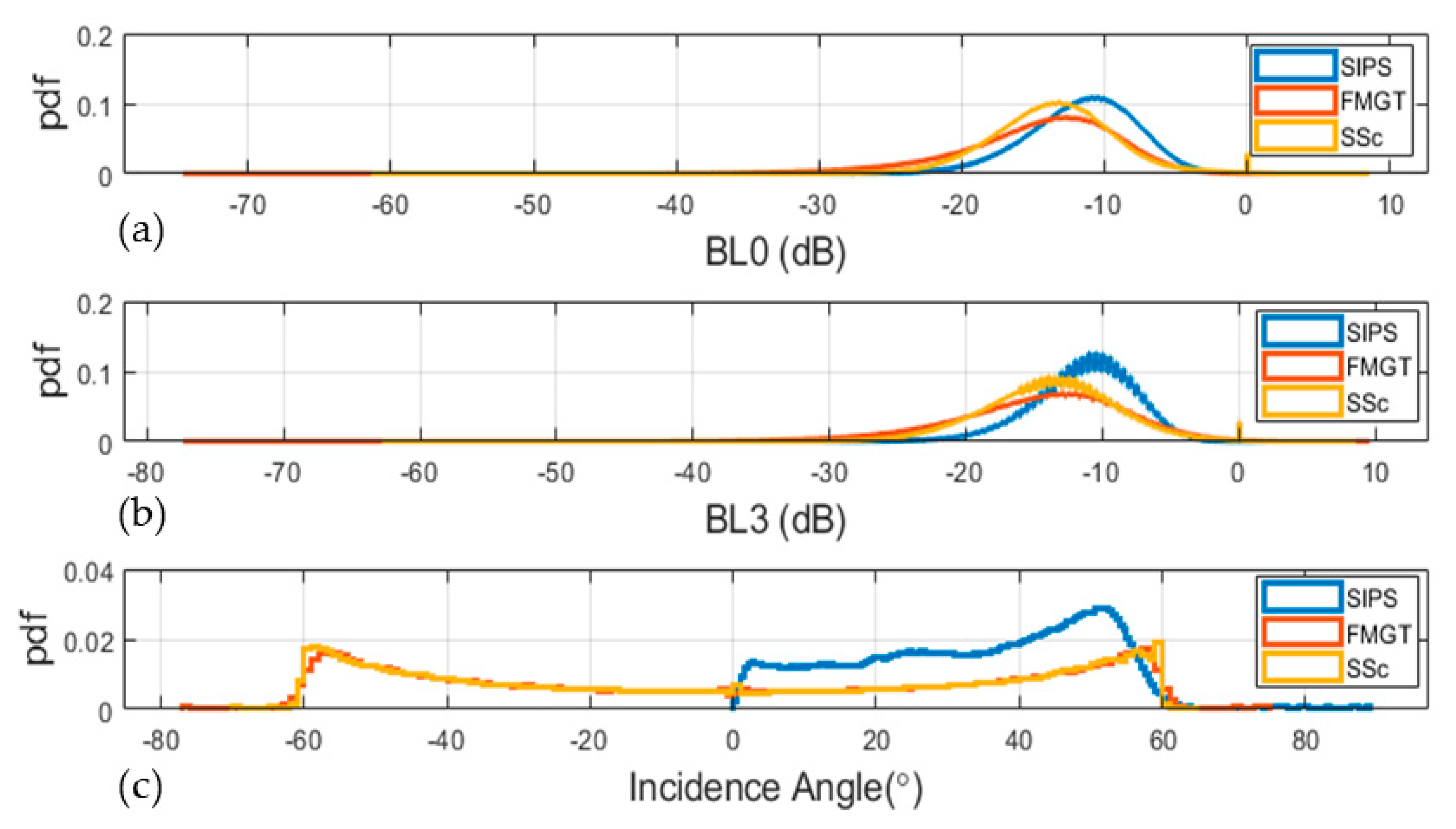
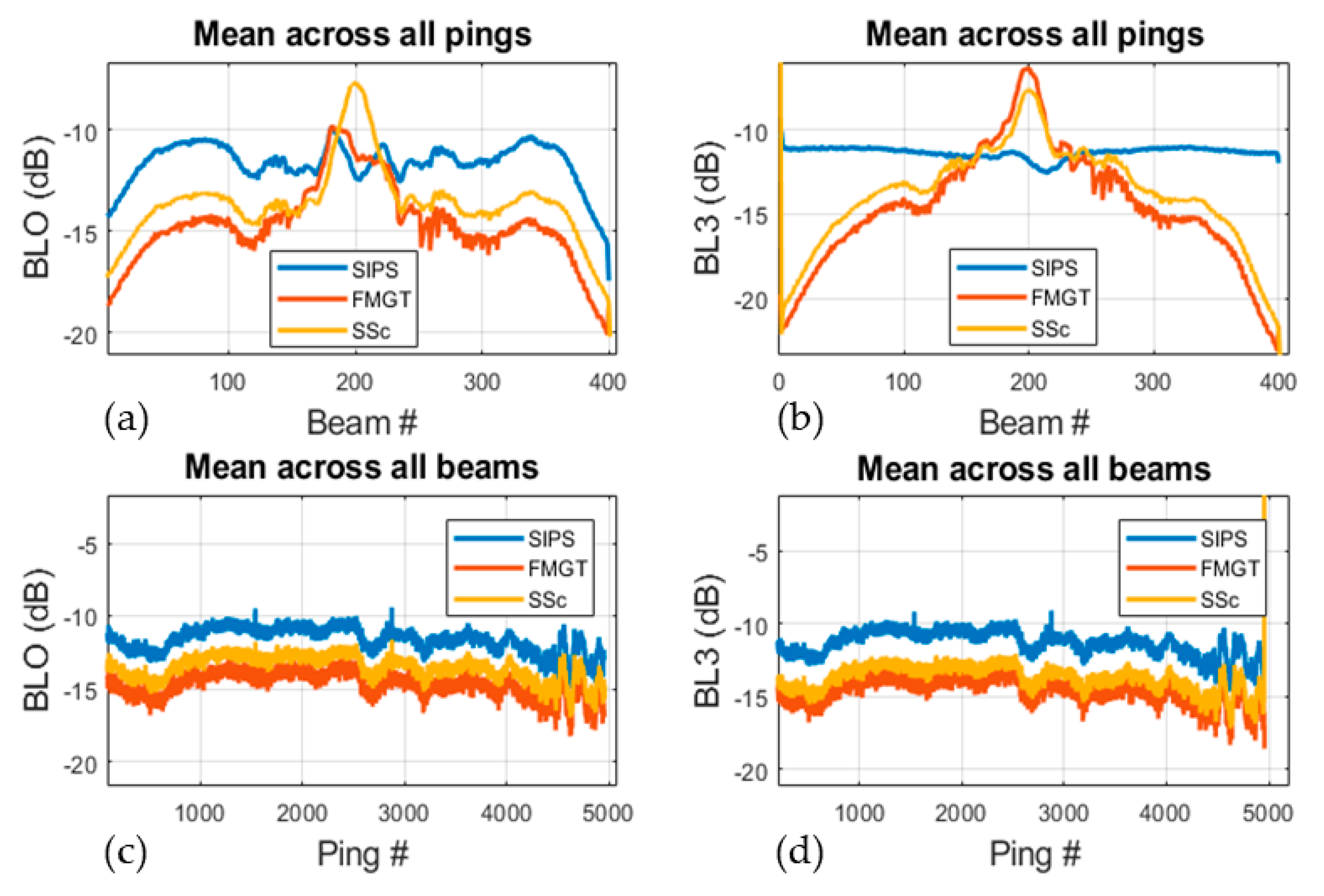
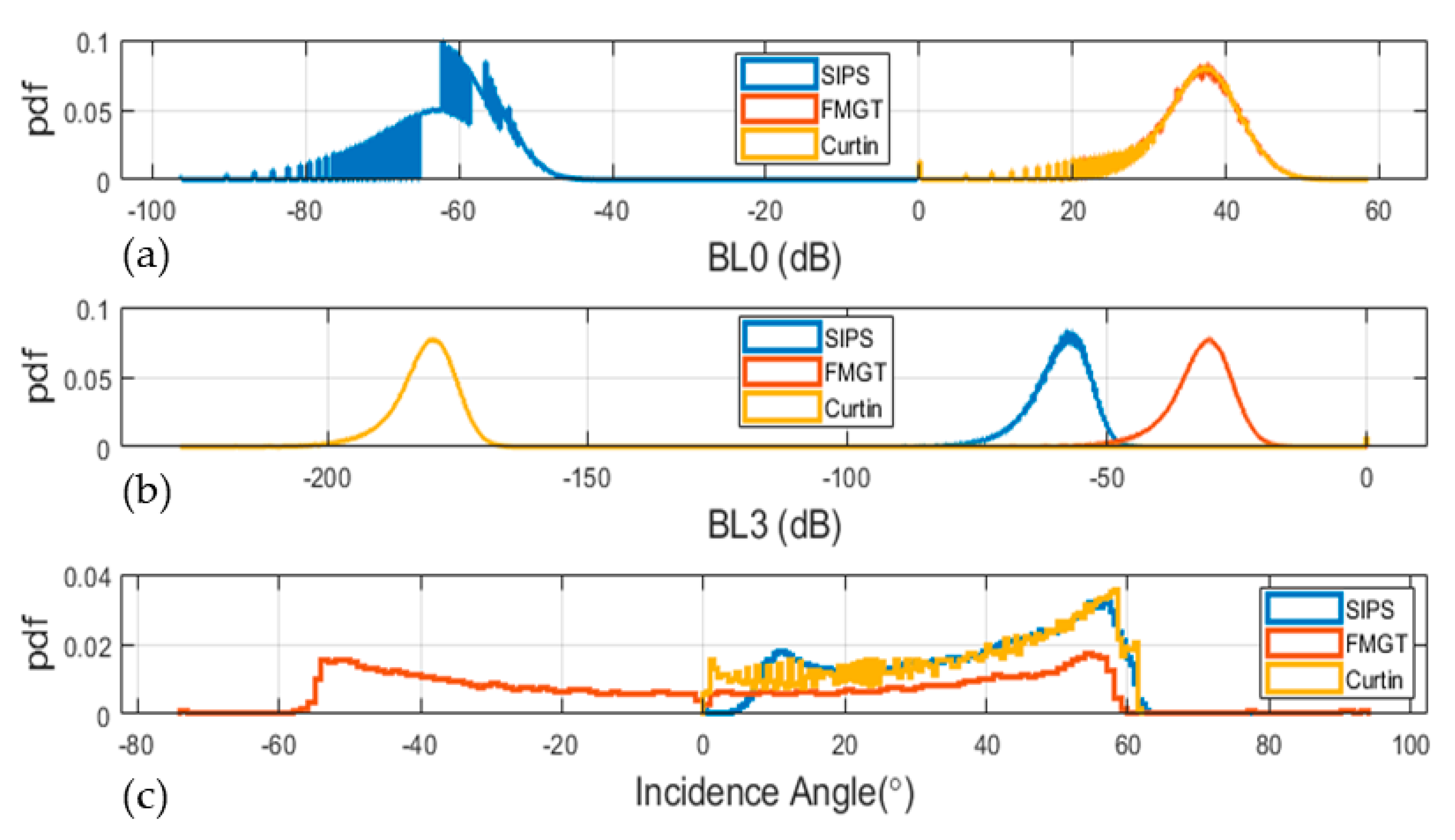
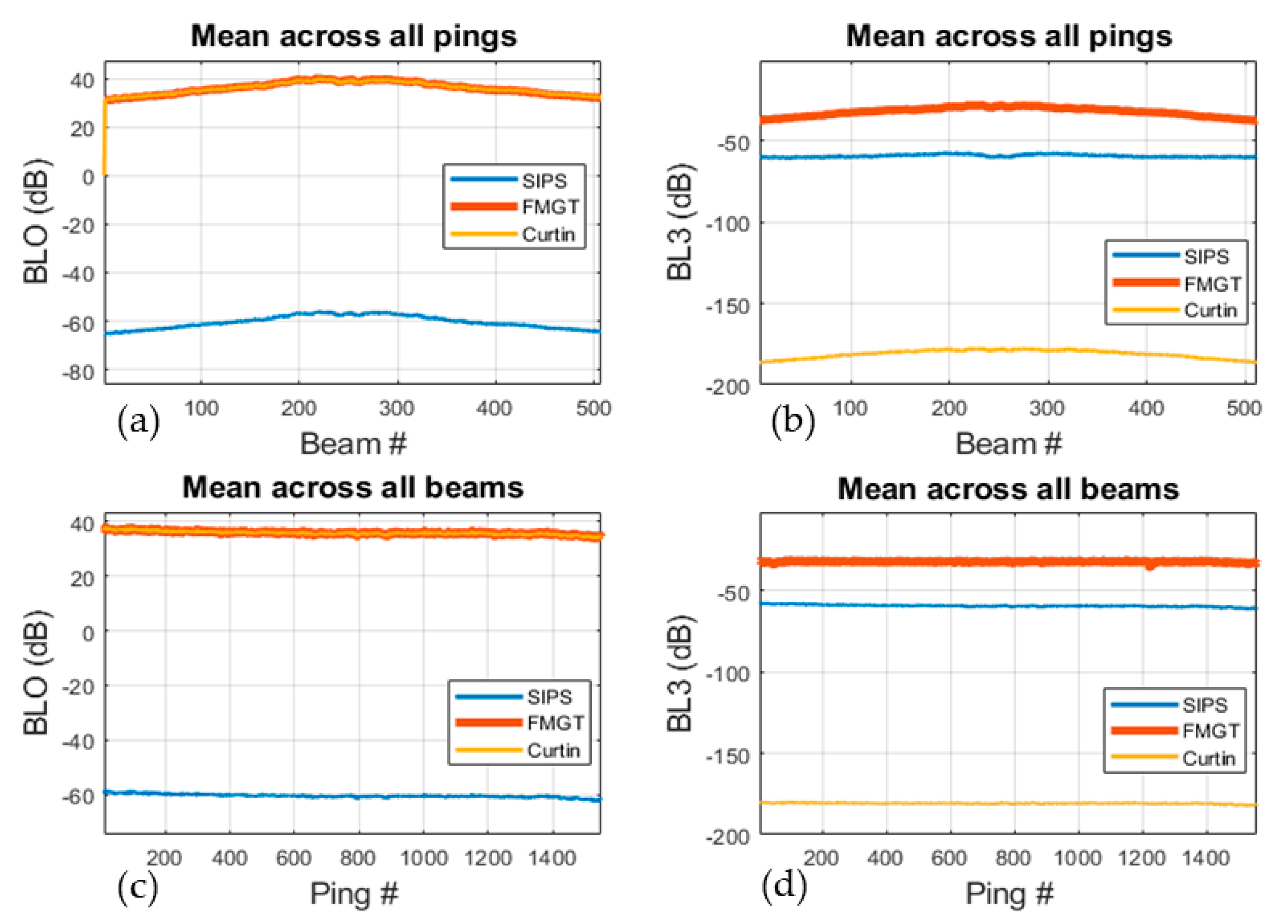
3.2. Comparison of BL0 and BL3

The software provided results whose patterns were qualitatively comparable but whose relative levels were often very different (BL0 in Figure 6 and BL3 in Figure 7). The mean values of BL0 and BL3 were computed for each beam and ping and showed that the differences between the tools could be larger than 5 dB (Figure 8). It was also evident these differences are not uniform across the swath. A pair-wise comparison revealed that the differences were more pronounced for the outer beams compared to near-nadir beams (Figure 9).

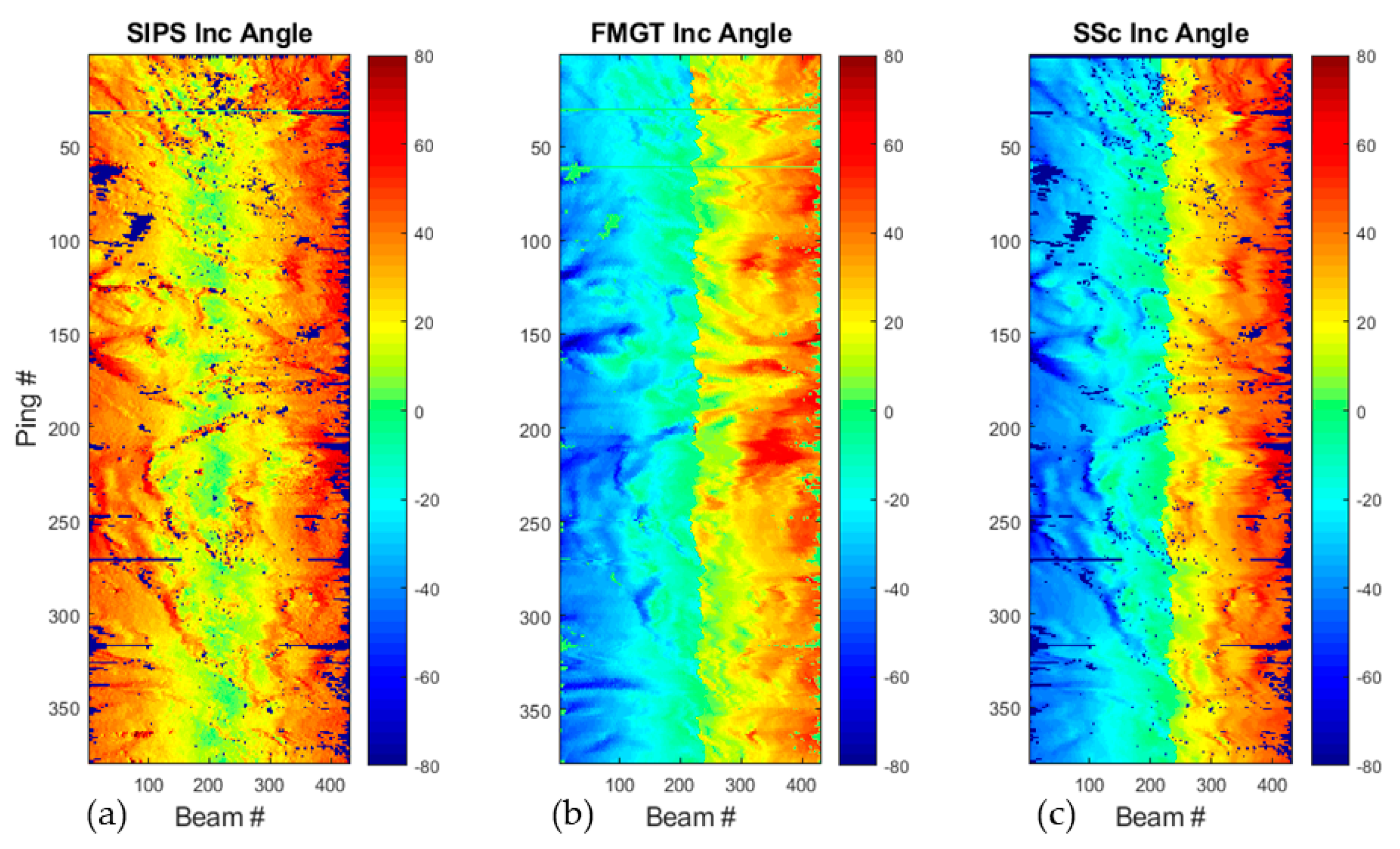
3.3. Comparison of Reported Incidence Angles

CARIS SIPS reported incidence angles were positive and ranged from 0° to 80° while FMGT and SonarScope reported the incidence angle with a range from −80° to 80° with port swath incidence angles reported as negative numbers (Figure 10 and Figure 11). Topographically-related variations in incidence angles are clearly visible in the output of SIPS, FMGT, and SonarScope, suggesting that seafloor slope was considered while computing the seafloor incidence angle. However, slight variations in the incidence angle are noticeable that may be related to the differences in the cleaning or smoothing of the DTM used to correct for seafloor slope.

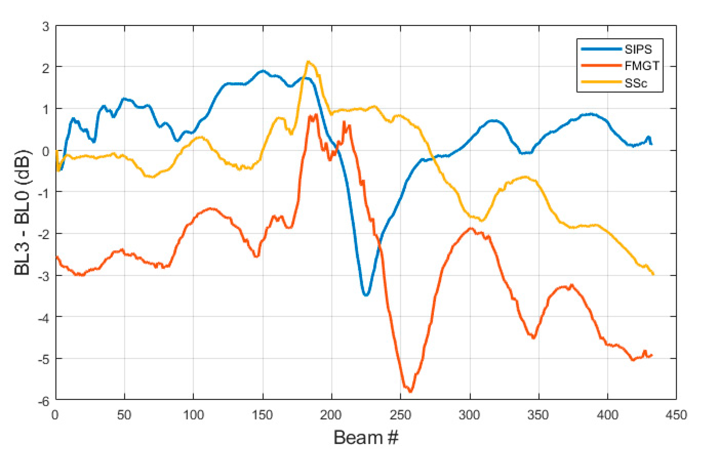
3.4. Comparison of Corrections Applied For BL3 Processing

The difference between BL3 and BL0 was computed for each software solution in order to obtain the total correction factor applied in the radiometric correction stage (Figure 12 and Figure 13). These show that each software applies very different processing corrections to arrive at BL3. In the case of SIPS, the correction appears as an along-track stripes pattern, which would implicate beam pattern correction (Section 2.3.1). In the case of FMGT, the correction is reminiscent of the incidence angle. In the case of SonarScope, the correction increases somewhat regularly away from nadir. Without the knowledge of the intermediate stages between BL0 and BL3 (BL2A and BL2B—See Figure 2), these interpretations are not definitive.

3.5. Summary of Differences Between Software for Different Sonar Types

In the previous sections, the differences between SIPS, FMGT, and SonarScope processing an EM302 data file were explored. In this section, the results of BL0, BL3, and incidence angle for other sonar types are summarized. The results show that EM 710 (Figure 14 and Figure 15), EM 3002 (Figure 16 and Figure 17), EM 2040 (Figure 18 and Figure 19), and SeaBat 7125 (Figure 20 and Figure 21) also present large differences.
The pairwise differences for both BL0 and BL3 results differ considerably among processing solutions for the example files from all sonar models. The mean differences (except for the SeaBat 7125 data file) ranged from ~2 dB to ~10 dB with standard deviations of up to 8 dB. For the Seabat 7125 data file, the mean of the difference between FMGT and MB Process results was <1 dB, but the difference was ~100 dB for comparisons involving SIPS. The large discrepancy observed in SIPS results for the SeaBat 7125 data file indicates the application of large offset while reading the snippets.

3.6. Relative Importance of Difference in Raw Data Reading (BL0) Compared to Radiometric Correction (BL3-BL0)

The results presented above showed that software solutions provided levels that differ both at the initial raw data reading stage (BL0) and after the radiometric correction have been applied (BL3). A few possible reasons for differences in BL0 will be discussed in Section 4.2.
The question arises as to whether the difference in the end results (BL3) is due mostly to the difference in data reading (BL0) or in radiometric corrections applied (BL3−BL0). To assess which of the two sources of differences contributes the most to the difference in end results, the absolute value of the ratio between the difference in radiometric correction and the difference in raw data reading (Equation (1), considering two software solutions A and B) was calculated:
γ = | [ B L 3 A B L 0 A ] [ B L 3 B B L 0 B ] [ B L 0 A B L 0 B ] | .
Small γ values (tending towards zero) indicate that the difference in end results is mostly due to differences in raw data reading. Conversely, large γ values (tending towards infinity) indicate that the difference in end results is mostly due to the difference in radiometric corrections. A γ value of 1 indicates that both sources of difference contribute equally to the difference in end results. In Table 3, we report for each dataset and each pair of software that could be, thus, compared, the median γ value and its interquartile range.
In the case of Kongsberg systems, the median γ value is almost always less than 1, indicating that for most datasets and most software comparisons, the difference in data reading has more influence on the difference in the end results than radiometric corrections. Only the SIPS/FMGT comparison on the EM710 dataset shows a median γ larger than 1, indicating, in this case, that difference in radiometric corrections have a (slightly) larger influence. The same analysis applied to the SeaBat 7125 data produced many different results. MB Process and FMGT read the SeaBat 7125 raw data very similarly, leading to a very large median γ value that confirms that the difference in end results is almost entirely due to the difference in radiometric corrections. However, SIPS reads the data differently than the two other software, and the difference in end result seems to be mostly due to this difference in data reading when compared with FMGT (median γ of 0.71), but mostly due to difference in radiometric processing when compared with MB Process (median γ of 2.27). Note that the interquartile ranges are often quite large, indicating that to obtain the future goal of consistent end results both of the two sources of difference will need to be addressed but the most important source of the differences in the end-results (except for MB Process and FMGT’s approach to processing SeaBat 7125 data), currently is simply due to the original choice of the starting value (BL0).

4. Discussion

MBES backscatter data are increasingly used to provide information about the nature of the seabed, in resource management projects, to assess the potential environmental impacts of human activities on the seabed, and for monitoring and managing marine habitats [8,10]. In many of such projects, it is often required to merge backscatter data from several sources, which often use different data processing and analysis software packages (e.g., EU national monitoring programs in relation with the EU Marine Strategic Framework Directive [27], Seamap Australia—a national seafloor habitat classification scheme [28] and Marine AREA database for Norwegian waters: MAREANO [29]). In this context, the quality control of the data and final products have important regulatory and legal implications. It is incumbent upon government agencies and scientific institutions to recognize that software packages used to process the raw data into useable products also impact the interpretation of these products and thus should be accredited for quality level [30]. There is a lot to gain for all the parties involved, to develop quality control approaches for the algorithms, and reach a level of standardization sufficient to merge the products from different software packages. The comparative analysis of intermediate software results, as developed in this paper, is a first step in the direction of processing standardization. We acknowledge that this study has been limited to analysis of data from a selection of commonly used MBES, and only a few backscatter processing packages. Future work of the BSIP/BSWG will incorporate data from a wider range of MBES, will facilitate the analysis of data logged in a variety of formats including Kongsberg’s new KMALL format for which software manufacturers are only starting to develop stable solutions at this time and hope to engage more backscatter processing software packages.

4.1. Importance of Accurate, Transparent, and Consistent Software Solutions in Science

The software solutions provide critical functionality to support data acquisition, processing, analysis, and visualization for nearly all the scientific disciplines, including benthic studies [31,32]. The choice of processing software is a critical decision. Software solutions may be chosen based on several criteria including accuracy, transparency, consistency, ease of use, price, fit for the specific processing needs, computing resources requirements, and compatibility with other tools being used by an organization and project partners. The determination of accuracy, transparency, and consistency of software solutions requires detailed testing that is beyond the scope of a single study such as the present one [33]. However, the unexplained differences between the backscatter results processed by the tools that are widely used by scientists is a concern shared by end-users of backscatter data, agencies funding data acquisition and processing; and software solution providers [34,35]. Hook and Kelley [33] identified a lack of quality control and means of comparing software output to expected and correct results as a critical challenge to assess a software package. The current study compares some of the intermediate processing results of non-transparent processing chains in an attempt to highlight which parts of these processing chains differ the most. Only four software solution providers participated in this study, but it is expected that future efforts will include other software packages. One very positive development has been that through this study and the cooperation of the software manufacturers, each of the three commercial software packages that were studied (QPS, CARIS, and SonarScope) now have the functionality to export intermediate results that will enable future end-users to be able to assess the processing chain themselves.

4.2. Why Do Different Approaches to Reading Raw Data Exist and Which One is Correct?

The results indicate that the raw data in the form of seabed image/snippets is read differently by various software to create what is termed as ‘beam averaged backscatter’ and was referred during this study as BL0. The impetus to compute beam averaged backscatter value stems from the need to reduce the statistical uncertainty of seafloor backscatter [6,15]. Through the commercial development of MBES, different approaches have been taken for the collection and provision of backscatter data, and these differences may offer some explanation for the discrepancies found. For instance, historically, the approaches taken to compute a single representative value per beam from recorded snippets differed based on:
  • Choice of central tendency, i.e., mean, median, or some other measure;
  • Choice of how the backscatter samples are selected to compute a measure of central tendency, e.g., use all the samples within a beam vs. using some threshold around the bottom detect to obtain a subset of samples vs. some other variations to choose samples;
  • Choice of the calculation method. MBES samples provided by sonar manufacturers represent backscatter strength in dB. These samples can be directly used to compute their central tendency, or they can be first converted into linear domain before calculating averages, and then the computed average converted back to a logarithmic scale.
For the purposes of this study, the software vendors were not required to disclose the details of their processing steps. The discussions over the course of this study with software developers indicated that this information might not be readily disclosed as the software developers are limited by non-disclosure agreements with hardware manufacturers from openly disclosing the internal processing of hardware. The information about the computation of BL0 for various software that could be obtained during the study is summarized in Table 4. The impact of these various choices will result in differences in the reported results depending on the specific data set and range of the recorded backscatter values. These differences are the most likely reasons the BL0 values reported for various tools were different. A recommendation to use one or the other approach based on rigorous analysis is beyond the scope of the current study, but further investigation into this issue should be prioritized in close collaboration with hardware manufacturers as well as software developers.

4.3. Need for Adoption of Metadata Standards

While MBES bathymetry data has long been subject to standards of accuracy [17], quantified uncertainties [36], and validated processing sequences, MBES backscatter mosaics are often considered qualitative products. The long-standing obstacle here is the complexity of the logistics of calibrating MBES backscatter data, and this situation has delayed the development and applications of the usage of this data-type [11]. The shift from a qualitative treatment of seafloor backscatter products such as backscatter mosaics to that of repeatable quantitative measurements may not be complete until feasible calibration procedures are developed, agreed upon, and routinely implemented. In the meantime, however, additional tools need to be made available to end-users to analyze the impact of their choices of parameters and algorithms in their backscatter data processing routine. Compilation of results from multisource multibeam echo sounders (e.g., [37]) and for multi-frequency systems (e.g., [38]) indicate the growing demand for consistent processing methodology. The ability to identify the reason(s) of differences in the processed results is, therefore, an essential component to understand if the differences in repeat or adjacent surveys are due to the seafloor changes, acquisition differences, or merely due to post-processing differences. This study reinforces the need for comprehensive metadata to accompany processed results [11]. In the absence of estimates of the accuracy or uncertainty of a data product (as is the case with MBES bathymetry), metadata provide the backscatter users with the minimum sufficient information to replicate the final product if necessary, and correct issues that may be discovered. Metadata also has an essential role in providing information to end-users (e.g., a geologist interpreting seabed sediment type) who may not be actively involved in, or have an in-depth knowledge of, backscatter processing yet whose perception of the data is influenced by the data provenance from acquisition through processing. The development and implementation of a standard metadata format for backscatter data products by the community (involving sonar manufacturers, software developers, and the users of this hardware and software across industry, academia, and government organizations) should, therefore, be a priority.

4.4. Collaboration between Backscatter Stakeholders

Our study reveals that much of the difference in backscatter results can be linked to a lack of communication between end-users, sonar manufacturers, and software developers. The current state where the results from different software packages are not reliable is a result of the independent evolution of methodology without considering end-users needs to be able to achieve consistent backscatter results irrespective of which software tool they use. This study has been conducted under the umbrella of the GEOHAB Backscatter Working Group (BSWG), which has been organized to provide a platform for academic, commercial, and government entities to collaborate to address challenges in backscatter processing. Although the calls for such collaborations have been numerous [39,40,41], collaborations focused on a specific data type (MBES backscatter) are rare. The lessons learned from the collaboration, which made the current study possible include:
  • The collaboration works well if all the stakeholders can communicate. BSWG provided an effective communication platform that facilitated the discussions.
  • Different entities may have different end goals in mind while collaborating on such projects. The framework of a successful collaboration depends on finding common goals. For example, in this case, the common goal was an improvement in the consistency of backscatter results, which motivated all stakeholders to agree to work closely. For other similar efforts, e.g., efforts to standardize seafloor backscatter segmentation and characterization, the identification of a common goal may not be very clear due to multiple divergent needs of end-users or desire to protect commercial interests.
  • Challenges of navigating proprietary restrictions both for multibeam echosounder software and hardware manufacturers are very real and may hamper successful collaboration between stakeholders [42].

5. Conclusions

The applications of seafloor backscatter data are expanding. To support such an expansion, there is a critical need for an increased output consistency among various software packages or, at least, a clear explanation for differences among software solutions. Hence, the progress made in this study was due to the cooperation of the software providers. For instance, during this study, significant differences were encountered between the outputs of several popular backscatter software packages, but through collaboration, a better understanding of where these differences were introduced in the processing pipeline was achieved. This study adapted the standard pipeline and nomenclature proposed by Schimel et al. [9] to produce the results from backscatter intermediate processing stages. However, the data from these intermediate processing stages are currently not produced consistently by all the software developers. Therefore, the active participation of software developers will be critical to make appropriate changes in the software packages to enable the export of results from intermediate processing stages while expanding this approach to other software packages.
Two intermediate processing levels were assessed during this study: the level read from the raw data files (BL0) and the level after radiometric corrections but before the removal of angular dependence (BL3). Software developers applied the required changes in their processing methodologies and provided data in Beam – Ping configuration with BL0 and BL3 reported for each beam along with incidence angle. Both BL0 and BL3 showed differences as high as >10 dB between the software packages. The differences in BL0 indicate that closed source software has adopted different approaches to read and reduce the raw data. These differences suggest this stage as one of the major causes of the observed differences in the final products. The observed discrepancy between BL0 calls for standardization of processing at this early stage of backscatter processing as well as more transparency from software providers to describe their computation choices. Critical choices of BL0 computation that should be targeted for developing a standard includes: (a) the choice of computation method for central tendency, i.e., mean or median; (b) the selection of samples used to compute BL0, and; (c) the choice of linear or logarithmic domain for computation.
This study has shown the applicability and usefulness of the availability of intermediate processing stages for the inter-comparison of proprietary software without requiring the software vendors to disclose their proprietary algorithms. Hence, although the scope of this study has been limited to understand the differences between the specific software package results, it adds weight to the argument of why it is critical for various sonar manufacturers, commercial, and academic software developers, and end-users from diverse domains to work together to develop methods that can improve the consistency of backscatter processing. It is evident from this, and several previous studies that accepted protocols to test and compare software processing results are desired. This study offers a first step towards the implementation of previously proposed processing protocols. As software developers start to offer the results from other intermediate processing stages, it can be envisioned that data test benches can be developed to aid end-users in evaluating various processing options currently available in processing tools [43].

Author Contributions

Conceptualization—M.M., A.C.G.S., G.M., M.R. and M.F.J.D.; Data curation—M.M., G.M, J.L.D., J.B., J.-M.A., T.H. and I.P.; Formal analysis—M.M., A.C.G.S. and G.M.; Methodology—M.M., A.C.G.S., G.M., M.R., J.L.D. and M.F.J.D.; Project administration—M.M., A.C.G.S., G.M., M.R., J.L.D. and M.F.J.D.; Software—J.B., J.-M.A., T.H. and I.P.; Supervision—M.M.; Writing—original draft—M.M.; Writing—review & editing—M.M., A.C.G.S., G.M., M.R., J.L.D., M.F.J.D., J.B., J.-M.A., T.H. and I.P.

Funding

This research received no external funding

Acknowledgments

Backscatter Working Group (BSWG) co-chair Xavier Lurton and Geoffrey Lamarche facilitated early discussions to setup the Backscatter Software Inter-comparison Project under the auspices of BSWG. We thank two anonymous reviewers whose comments greatly improved this manuscript.

Conflicts of Interest

The following authors declare that they have no known competing financial interests or personal relationships that could have appeared to influence the work reported in this paper: Mashkoor Malik, Alexandre C. G. Schimel, Giuseppe Masetti, Marc Roche, Julian Le Deunf, Margaret F.J. Dolan. The following authors declare the following financial interests/personal relationships which may be considered as potential competing interests: Travis Hamilton is employed at Teledyne CARIS which produces HIPS and SIPS, a software package used in this inter-comparison study; Jonathan Beaudoin is employed at QPS which produces FMGT, a software package used in this inter-comparison study; Jean-Marie Augustin is employed at IFREMER which produces SonarScope, a software package used in this inter-comparison study; and Iain Parnum is employed at Curtin University which produces MB Process, a software package used in this inter-comparison study.

Disclaimer

The scientific results and conclusions, as well as any views or opinions expressed herein are those of the author(s) and do not necessarily reflect the views of the National Ocean and Atmospheric Administration (NOAA); the Department of Commerce; the National Institute of Water and Atmospheric Research (NIWA), the University of New Hampshire, the Federal Public Service Economy of Belgium (FPSE), the Service Hydrographique et Océanographique de la Marine (SHOM), the Geological Survey of Norway (NGU), QPS, CARIS Teledyne, IFREMER or Curtin University. Mention of a commercial company or product does not constitute an endorsement by host agencies of author(s). The comparison results have been developed in close collaboration with CARIS, QPS, IFREMER and Curtin University and published with their permission. These comparison results were focused only on developing intermediate backscatter processing stages and did not address software usability, bathymetry processing and other features that prospective users of these software packages may also want to consider.

Appendix A

Table A1. List of the data files used during this study.
Sonar TypeData File
EM 3020213_20170717_112534_EX1706_MB.all
EM 7100002_20130214_091514_borda.all
EM 30020009_20100113_121654_guillemot.all
EM 20400005_20160412_104116_SimonStevin.all
SeaBat 712520140729_082527_SMB Owen.s7k

Appendix B

Table A2. Number of columns, and relevant column names in the ASCII files exported from each software.
SoftwareSonarScopeFMGTCARIS SIPSMB Process
# columns31121711
Time stamp (Unix Time)Time UTC Ping TimeTimestampPing Time
Ping #PingPing NumberPingPing Number
Beam #BeamBeam NumberBeamBeam Number
Beam location (Lat/Long)Latitude/LongitudeLatitude/LongitudeLongitude/LatitudeLongitude/Latitude
Beam location (E/N)GeoX/GeoYEasting/NorthingEasting/NorthingEasting/Northing
Beam depthBathyRTDepthDepth(Not Provided)
Incidence angle IncidenceAnglesTrue AngleIncidentAngleIncidence Angle
BS as read from data files (BL0)ReflecSScBackscatter ValueBL0Backscatter value
BS processed angular response (BL3)SSc_Step1Corrected Backscatter ValueBL3Corr Backscatter Value
Data processedAll except SeaBat 7125All except EM 3002AllOnly SeaBat 7125

References

  1. de Moustier, C. State of the art in swath bathymetry survey systems. Int. Hydrogr. Rev. 1988, 65, 25–54. [Google Scholar]
  2. Hughes Clarke, J.E.; Mayer, L.A.; Wells, D.E. Shallow-water imaging multibeam sonars: A new tool for investigating seafloor processes in the coastal zone and on the continental shelf. Mar. Geophys. Res. 1996, 18, 607–629. [Google Scholar] [CrossRef]
  3. de Moustier, C. Beyond bathymetry: Mapping acoustic backscattering from the deep seafloor with Sea Beam. J. Acoust. Soc. Am. 1986, 79, 316–331. [Google Scholar] [CrossRef]
  4. Mayer, L.A. Frontiers in Seafloor Mapping and Visualization. Mar. Geophys. Res. 2006, 27, 7–17. [Google Scholar] [CrossRef]
  5. Anderson, J.T.; Holliday, D.V.; Kloser, R.; Reid, D.; Simard, Y.; Brown, C.J.; Chapman, R.; Coggan, R.; Kieser, R.; Michaels, W.L.; et al. ICES Acoustic Seabed Classification of Marine Physical and Biological Landscapes; ICES Cooperative Research Report No. 286; International Council for the Exploration of the Sea Conseil, International pour l’Exploration de la Mer: Copenhagen, Denmark, August 2007. [Google Scholar]
  6. Jackson, D.R.; Richardson, M.D. High-Frequency Seafloor Acoustics; Springer Science & Business Media: New York, UK, 2007; ISBN 978-0-387-34154-5. [Google Scholar]
  7. Lurton, X. An Introduction to Underwater Acoustics: Principles and Applications, 2nd ed.; Springer: Berlin/Heidelberg, Germany, 2010; ISBN 978-3-540-78480-7. [Google Scholar]
  8. Lucieer, V.; Roche, M.; Degrendele, K.; Malik, M.; Dolan, M.; Lamarche, G. User expectations for multibeam echo sounders backscatter strength data-looking back into the future. Mar. Geophys. Res. 2018, 39, 23–40. [Google Scholar] [CrossRef]
  9. Schimel, A.C.G.; Beaudoin, J.; Parnum, I.M.; Le Bas, T.; Schmidt, V.; Keith, G.; Ierodiaconou, D. Multibeam sonar backscatter data processing. Mar. Geophys. Res. 2018, 39, 121–137. [Google Scholar] [CrossRef]
  10. Lurton, X.; Lamarche, G.; Brown, C.; Lucieer, V.; Rice, G.; Schimel, A.C.G.; Weber, T.C. Backscatter Measurements by Seafloor-Mapping Sonars—Guidelines and Recommendations. Geohab report. May 2015. Available online: http://geohab.org/wp-content/uploads/2013/02/BWSG-REPORT-MAY2015.pdf (accessed on 10 November 2019).
  11. Lamarche, G.; Lurton, X. Recommendations for improved and coherent acquisition and processing of backscatter data from seafloor-mapping sonars. Mar. Geophys. Res. 2018, 39, 5–22. [Google Scholar] [CrossRef] [Green Version]
  12. Dufek, T. Backscatter Analysis of Multibeam Sonar Data in the Area of the Valdivia Fracture Zone using Geocoder in CARIS HIPS&SIPS and IVS3D Fledermaus. Master’s Thesis, Hafencity University Hamburg, Hamburg, Germany, 2012. [Google Scholar]
  13. Roche, M.; Degrendele, K.; Mol, L.D. Constraints and limitations of MBES Backscatter Strength (BS) measurements for monitoring the seabed. Surveyor and geologist point of view. In Proceedings of the GeoHab (Maine Geological and Biological Habitat Mapping), Rome, Italy, 6–10 May 2013; p. 21. [Google Scholar]
  14. Roche, M.; Degrendele, K.; Vrignaud, C.; Loyer, S.; Le Bas, T.; Augustin, J.-M.; Lurton, X. Control of the repeatability of high frequency multibeam echosounder backscatter by using natural reference areas. Mar. Geophys. Res. 2018, 39, 89–104. [Google Scholar] [CrossRef] [Green Version]
  15. Malik, M.; Lurton, X.; Mayer, L. A framework to quantify uncertainties of seafloor backscatter from swath mapping echosounders. Mar. Geophys. Res. 2018, 39, 151–168. [Google Scholar] [CrossRef] [Green Version]
  16. Malik, M. Sources and impacts of bottom slope uncertainty on estimation of seafloor backscatter from swath sonars. Geosciences 2019, 9, 183. [Google Scholar] [CrossRef] [Green Version]
  17. Hare, R.; Godin, A.; Mayer, L.A. Accuracy Estimation of Canadian Swath (Multibeam) and Sweep (Multitransducer) Sounding Systems; Canadian Hydrographic Service Internal Report; Canadian Hydrographic Service: Ottawa, ON, Canada, 1995. [Google Scholar]
  18. FMGT—Fledermaus Geocoder Toolbox 7.8.0; Quality Positioning Services BV (QPS): Zeist, The Netherlands, 2018.
  19. Teledyne Computer Aided Resource Information System (CARIS) HIPS and SIPS; Teledyne CARIS Inc.: Fredericton, NB, Canada, 2019.
  20. Augustin, J. SonarScope® software on-line presentation. Available online: http://flotte.ifremer.fr/fleet/Presentation-of-the-fleet/Logiciels-embarques/SonarScope (accessed on 6 June 2019).
  21. Kongsberg Inc. Kongsberg Multibeam Echo Sounder EM Datagram Formats. Rev. W. Available online: https://www.kongsberg.com/globalassets/maritime/km-products/product-documents/160692_em_datagram_formats.pdf (accessed on 15 November 2019).
  22. Teledyne Reson Teledyne Reson Data Format Definition Document. 7k Data Format, Volume 1, Version 3.01. Available online: https://www.teledyne-pds.com/wp-content/uploads/2016/11/DATA-FORMAT-DEFINITION-DOCUMENT-7k-Data-Format-Volume-I-Version-3.01.pdf (accessed on 20 June 2019).
  23. Kongsberg Inc. KMALL Datagram description Rev:F. Available online: https://www.kongsberg.com/maritime/support/document-and-downloads/software-downloads/ (accessed on 15 June 2019).
  24. Gavrilov, A.; Duncan, A.; McCauley, R.; Parnum, I.; Penrose, J.; Siwabessy, P.; Woods, A.J.; Tseng, Y.-T. Characterization of the seafloor in Australia’s coastal zone using acoustic techniques. In Proceedings of the 1st International Conference on Underwater Acoustic Measurements, Heraklion, Greece, 28 June–1 July 2005; pp. 1075–1080. [Google Scholar]
  25. Parnum, I.M.; Tyler, E.; Miles, P. Software for rapid visualisation and analysis of multibeam echosounder water column data. In Proceedings of the ICES Symposium on Marine Ecosystem Acoustics, Nantes, France, 25–28 May 2015. [Google Scholar]
  26. Parnum, I.M.; Gavrilov, A.N. High-frequency multibeam echo-sounder measurements of seafloor backscatter in shallow water: Part 1—Data acquisition and processing. Underw. Technol. 2011, 30, 3–12. [Google Scholar] [CrossRef]
  27. European Parliament; Council of the European Union. Directive 2008/56/EC of the European Parliament and of the Council of 17 June 2008 Establishing a Framework for Community Action in the Field of Marine Environmental Policy (Marine Strategy Framework Directive) (Text with EEA Relevance); 2008. Available online: http://www.legislation.gov.uk/eudr/2008/56/2019-10-31# (accessed on 10 November 2019).
  28. Lucieer, V.; Walsh, P.; Flukes, E.; Butler, C.; Proctor, R.; Johnson, C. Seamap Australia—A National Seafloor Habitat Classification Scheme; Institute for Marine and Antarctic Studies (IMAS), University of Tasmania: Hobart TAS, Australia, 2017. [Google Scholar]
  29. Buhl-Mortensen, L.; Buhl-Mortensen, P.; Dolan, M.F.J.; Holte, B. The MAREANO programme—A full coverage mapping of the Norwegian off-shore benthic environment and fauna. Mar. Biol. Res. 2015, 11, 4–17. [Google Scholar] [CrossRef]
  30. Manzella, G.; Griffa, A.; de la Villéon, L.P. Report on Data Management Best Practice and Generic Data and Metadata Models. V.2.1 [Deliverable 5.9]; Ifremer for JERICO-NEXT Project: Issy-les-Moulineaux, France, 2017. [Google Scholar]
  31. Idaszak, R.; Tarboton, D.G.; Yi, H.; Christopherson, L.; Stealey, M.J.; Miles, B.; Dash, P.; Couch, A.; Spealman, C.; Horsburgh, J.S.; et al. HydroShare—A Case Study of the Application of Modern Software Engineering to a Large Distributed Federally-Funded Scientific Software Development Project. In Software Engineering for Science; Taylor & Francis CRC Press: Boca Raton, FL, USA, 2017; pp. 253–270. [Google Scholar]
  32. Hannay, J.E.; MacLeod, C.; Singer, J.; Langtangen, H.P.; Pfahl, D.; Wilson, G. How do scientists develop and use scientific software? In Proceedings of the 2009 ICSE Workshop on Software Engineering for Computational Science and Engineering, Washington, DC, USA, 23 May 2009; pp. 1–8. [Google Scholar]
  33. Hook, D.; Kelly, D. Testing for trustworthiness in scientific software. In Proceedings of the 2009 ICSE Workshop on Software Engineering for Computational Science and Engineering, Washington, DC, USA, 23 May 2009; pp. 59–64. [Google Scholar]
  34. Howison, J.; Deelman, E.; McLennan, M.J.; Ferreira da Silva, R.; Herbsleb, J.D. Understanding the scientific software ecosystem and its impact: Current and future measures. Res. Eval. 2015, 24, 454–470. [Google Scholar] [CrossRef] [Green Version]
  35. Carver, J.; Hong, N.P.C.; Thiruvathukal, G.K. Software Engineering for Science; Taylor & Francis CRC Press: Boca Raton, FL, USA, 2017; ISBN 978-1-4987-4385-3. [Google Scholar]
  36. Calder, B.R.; Mayer, L.A. Automatic processing of high-rate, high-density multibeam echosounder data. Geochem. Geophys. Geosyst. 2003, 4, 1048. [Google Scholar] [CrossRef]
  37. Hughes Clarke, J.E.; Iwanowska, K.K.; Parrott, R.; Duffy, G.; Lamplugh, M.; Griffin, J. Inter-calibrating multi-source, multi-platform backscatter data sets to assist in compiling regional sediment type maps: Bay of Fundy. In Proceedings of the Canadian Hydrographic and National Surveyors’ Conference, Victoria Conference Centre, Victoria, BC, Canada, 5–8 May 2008; p. 23. [Google Scholar]
  38. Feldens, P.; Schulze, I.; Papenmeier, S.; Schönke, M.; Schneider von Deimling, J. Improved interpretation of marine sedimentary environments using multi-frequency multibeam backscatter data. Geosciences 2018, 8, 214. [Google Scholar] [CrossRef]
  39. Pendleton, L.H.; Beyer, H.; Estradivari; Grose, S.O.; Hoegh-Guldberg, O.; Karcher, D.B.; Kennedy, E.; Llewellyn, L.; Nys, C.; Shapiro, A.; et al. Disrupting data sharing for a healthier ocean. ICES J. Mar. Sci. 2019, 76, 1415–1423. [Google Scholar] [CrossRef]
  40. Franken, S.; Kolvenbach, S.; Prinz, W.; Alvertis, I.; Koussouris, S. CloudTeams: Bridging the gap between developers and customers during software development processes. Procedia Comput. Sci. 2015, 68, 188–195. [Google Scholar] [CrossRef]
  41. Mackenzie, B.; Celliers, L.; de Freitas Assad, L.P.; Heymans, J.J.; Rome, N.; Thomas, J.; Anderson, C.; Behrens, J.; Calverley, M.; Desai, K.; et al. The role of stakeholders in creating societal value from coastal and ocean observations. Front. Mar. Sci. 2019, 6, 137. [Google Scholar] [CrossRef] [Green Version]
  42. Legendre, P. Reply to the comment by Preston and Kirlin on “Acoustic seabed classification: Improved statistical method”. Can. J. Fish. Aquat. Sci. 2003, 60, 1301–1305. [Google Scholar] [CrossRef] [Green Version]
  43. Masetti, G.; Augustin, J.M.; Malik, M.; Poncelet, C.; Lurton, X.; Mayer, L.A.; Rice, G.; Smith, M. The Open Backscatter Toolchain (OpenBST) project: Towards an open-source and metadata-rich modular implementation. In Proceedings of the US Hydro, Biloxi, MS, USA, 19–21 March 2019. [Google Scholar] [CrossRef]
Figure 1. Visual workflow of the backscatter data processing pipeline (adapted from Figure 1 in [9]), resulting in the two common backscatter products—angular response curves and mosaic. Only the BL0 and BL3 intermediate outputs were requested from software developers during the current study.
Geosciences 09 00516 g001
Figure 2. CARIS SIPS mosaic creation tool showing the advanced settings where a folder can be set for export of the text file that contains intermediate backscatter processed levels. CARIS SIPS ver. 11.1.3 (Released March 2019).
Geosciences 09 00516 g002
Figure 3. (a) The QPS FMGT settings that are available in version 7.8.0 (released December 2016). To enable export of the ARA Beam detail, flag ‘Keep data for ARA analysis’ in the processing parameters. (b) The ‘ASCII ARA Beam Detail’ export is available through the contextual display on the main window.
Geosciences 09 00516 g003
Figure 4. The interface in the SonarScope to select the export of .csv and .html files that provide details of the various corrections applied to produce processed backscatter results. SonarScope version 20190702_R2017b (released 2 July 2019).
Geosciences 09 00516 g004
Figure 5. Percentage of beams flagged as “invalid” by each software of the EM 302 data.
Geosciences 09 00516 g005
Figure 6. Plots showing BL0 results from (a) CARIS SIPS, (b) FMGT, and (c) SonarScope for the EM 302 data.
Geosciences 09 00516 g006
Figure 7. Plots showing BL3 results from (a) CARIS SIPS, (b) FMGT, and (c) SonarScope for the EM 302 data.
Geosciences 09 00516 g007
Figure 8. Plots showing BL0 (a,c) and BL3 (b,d) from CARIS SIPS, FMGT, and SonarScope for the EM 302 data. The plots on top (a,b) show the average over the entire survey line for all pings reported at each beam. The lower plots (c,d) show the average of all beams for each ping.
Geosciences 09 00516 g008
Figure 9. Mean and standard deviation of pair-wise differences in BL0 and BL3 from different software, as a function of beam number for the EM 302 data. (a) Mean of the BL0 differences, (b) standard deviation of the BL0 differences (c) Mean of the BL3 differences, and (d) standard deviation of the BL3 differences.
Geosciences 09 00516 g009
Figure 10. Plot showing the incidence angle reported for each beam by (a) CARIS SIPS, (b) FMGT, and (c) SonarScope for the EM 302 data.
Geosciences 09 00516 g010
Figure 11. Comparison of empirical probability density function (pdf) of (a) BL0, (b) BL3, and (c) Incidence angle from the three software packages for the EM 302 data.
Geosciences 09 00516 g011
Figure 12. Plots showing the total radiometric corrective factor (BL3−BL0) from (a) CARIS SIPS, (b) FMGT, and (c) SonarScope for the EM 302 data.
Geosciences 09 00516 g012
Figure 13. Plot showing the average corrective factor (BL3−BL0) per beam over 50 pings (pings # 100–150) for the EM 302 data.
Geosciences 09 00516 g013
Figure 14. Comparison of empirical probability density function (pdf) of (a) BL0, (b) BL3 and (c) incidence angle from FMGT, CARIS and Sonar Scope for the EM 710 data.
Geosciences 09 00516 g014
Figure 15. Plots showing BL0 (a,c) and BL3 (b,d) from CARIS SIPS, FMGT, and SonarScope for the EM 710 data. The plots on top (a,b) show the average over the entire survey line for all pings reported at each beam. The lower plots (c,d) show the average of all beams for each ping. SonarScope BL3 results were clipped for the pings where there was no reference DTM available.
Geosciences 09 00516 g015
Figure 16. Comparison of empirical probability density function (pdf) of (a) BL0, (b) BL3, and (c) incidence angle results from CARIS SIPS, FMGT, and Sonar Scope for the EM 3002 data file.
Geosciences 09 00516 g016
Figure 17. Plots showing BL0 (a,c) and BL3 (b,d) from CARIS SIPS, FMGT, and SonarScope for the EM 3002 data. The plots on top (a,b) show the average over the entire survey line for all pings reported at each beam. The lower plots (c,d) show the average of all beams for each ping. SonarScope BL3 results were clipped for the pings where there was no reference DTM available.
Geosciences 09 00516 g017
Figure 18. Comparison of the empirical probability density function (pdf) of (a) BL0, (b) BL3, and (c) incidence angle results from CARIS SIPS, FMGT, and Sonar Scope for the EM 2040 data.
Geosciences 09 00516 g018
Figure 19. Plots showing BL0 (a,c) and BL3 (b,d) from CARIS SIPS, FMGT and SonarScope for the EM 2040 data. The plots on top (a,b) show the average over the entire survey line for all pings reported at each beam. The lower plots (c,d) show the average of all beams for each ping.
Geosciences 09 00516 g019
Figure 20. Comparison of the empirical probability density function (pdf) of (a) BL0, (b) BL3, and (c) incidence angle results from FMGT, CARIS, and Curtin University MB Process for the SeaBat 7125 data.
Geosciences 09 00516 g020
Figure 21. Plots showing BL0 (a,c) and BL3 (b,d) from CARIS SIPS, FMGT, and Curtin University MB Process for the SeaBat 7125 data. The plots on top (a,b) show the average over the entire survey line for all pings reported at each beam. The lower plots (c,d) show the average of all beams for each ping.
Geosciences 09 00516 g021
Table 1. Datasets used during the study.
Echosounder Model
(Nominal Frequency)
VesselData Acquisition SoftwareAgencyLocationWeatherDateDepth Range
EM 2040
(300 kHz)
RV Simon StevinSISFPS EconomyKwinte reference area (Belgium)Calm12 April 201623–26 m
EM 3002
(300 kHz)
HSL GuillemotSISSHOMCarre Renard area,
Brest Bay, France
Calm13 Jan 201018–22 m
EM 710
(70–100 kHz)
BH2 BordaSISSHOMCarre Renard area, Brest Bay, FranceCalm14 Feb 201318–22 m
EM 302
(30 kHz)
NOAA Ship Okeanos ExplorerSISNOAAJohnston Atoll near Hawaii, USARough17 July 2017~3000 m
Reson SeaBat 7125
(400 kHz)
HMSMB OwenPDS2000Shallow survey common dataset 2015Plymouth, UKCalm29 July 2014<10 m
Table 2. Requested variables to be included in the ASCII export files for this study.
Column #12345678
Value reportedPing #Beam #Ping Time (Unix time)LatitudeLongitudeBL0Seafloor Incidence angle (BL3)BL3
Table 3. Median of γ and interquartile range Q3–Q1 (in parentheses), computed for various pairs of software processing the same dataset.
SIPS/FMGTFMGT/SonarScopeSonarScope/SIPSMB Process/FMGTMB Process/SIPS
EM3020.66 (1.23) 0.57 (1.12)0.39 (0.87)--
EM7101.19 (2.28)0.63 (1.02)0.80 (1.68)--
EM30020.63 (1.43)0.04 (0.13)0.94 (2.1)--
EM20400.3 (0.73)0.04 (0.11)0.31 (0.76)--
SeaBat71250.71 (0.04)--55.98 (148.9)2.27(0.16)
Table 4. Disclosed information by software packages to compute BL0. The information is produced here with the permission from the software packages.
CARIS SIPSFMGTSonar ScopeCurtin Univ. MB Process
Reson Systems:
Use the snippet sample associated with the bottom detection. Divide the stored value by 65536 (to convert from 2 byte to floating point) before applying the 20log10.

Kongsberg systems:
Fit a curve to snippet samples using a moving window (size 11 samples). Report the max value of the fit curve.
Reson and Kongsberg systems:
Identify all the samples that fall within ±5 dB around the bottom detect echo level and compute an average of these qualifying samples using the amplitude values in dB as reported in the datagram.
Kongsberg systems:
Use all of the full-time series samples recorded within a beam to compute an average value. By default, samples are first converted to energy (linear domain) before computing average and returned in dB. The new release (2019) provides the option to compute this value in dB, energy, median, or amplitude. The new default method is now in amplitude.
Reson systems:
Calculate the mean of samples that fall within ±5 dB around the bottom detect echo level.

