Article

Sentinel-1 for Monitoring Land Subsidence of Coastal Cities in Africa Using PSInSAR: A Methodology Based on the Integration of SNAP and StaMPS

by
Fabio Cian
1,2,*,
José Manuel Delgado Blasco
3 and
Lorenzo Carrera
1
1
The World Bank Group, Washington, DC 20433, USA
2
Department of Economics, Ca’ Foscari University Venice, 30121 Venice, Italy
3
Grupo de Investigación Microgeodesia, University of Jaén, 23071 Jaén, Spain
*
Author to whom correspondence should be addressed.
Geosciences 2019, 9(3), 124; https://doi.org/10.3390/geosciences9030124
Submission received: 13 January 2019 / Revised: 4 March 2019 / Accepted: 5 March 2019 / Published: 12 March 2019
(This article belongs to the Special Issue River, Urban, and Coastal Flood Risk)

Abstract

:
The sub-Saharan African coast is experiencing fast-growing urbanization, particularly around major cities. This threatens the equilibrium of the socio-ecosystems where they are located and on which they depend: underground water resources are exploited with a disregard for sustainability; land is reclaimed from wetlands or lagoons; built-up areas, both formal and informal, grow without adequate urban planning. Together, all these forces can result in land surface deformation, subsidence or even uplift, which can increase risk within these already fragile socio-ecosystems. In particular, in the case of land subsidence, the risk of urban flooding can increase significantly, also considering the contribution of sea level rise driven by climate change. Monitoring such fast-changing environments is crucial to be able to identify key risks and plan adaptation responses to mitigate current and future flood risks. Persistent scatterer interferometry (PSI) with synthetic aperture radar (SAR) is a powerful tool to monitor land deformation with high precision using relatively low-cost technology, also thanks to the open access data of Sentinel-1, which provides global observations every 6 days at 20-m ground resolution. In this paper, we demonstrate how it is possible to monitor land subsidence in urban coastal areas by means of permanent scatterer interferometry and Sentinel-1, exploiting an automatic procedure based on an integration of the Sentinel Application Platform (SNAP) and the Stanford Method for Persistent Scatterers (StaMPS). We present the results of PSI analysis over the cities of Banjul (the Gambia) and Lagos (Nigeria) showing a comparison of results obtained with TerraSAR-X, Constellation of Small Satellites for the Mediterranean Basin Observation (COSMO-SkyMed) and Environmental Satellite advanced synthetic aperture radar (Envisat-ASAR) data. The methodology allows us to highlight areas of high land deformation, information that is useful for urban development, disaster risk management and climate adaptation planning.

1. Introduction

Roughly 10% of the world’s population lives in low elevation zones, which, under climate change and rising sea levels, are at increasing risk of flooding [1]. Sea level has been rising by an average of 1.7 ± 0.3 mm/year since 1950 [2] and from the 1990s this has sped up, reaching a velocity of 3.3 ± 0.4 mm/year [3]. On average, this has led to a rise of more than 10 cm in about 60 years, with projections of future sea level rise of 1 m or more by 2100 [4,5]. The two main causes of sea level rise are connected to the thermal expansion of seawater due to ocean warming and water input from land ice melt [6]. In some coastal areas, sea level rise associated with storm surges can increase the magnitude and frequency of coastal flooding events. The impacts of these events can be locally amplified by anthropogenic processes like oil or groundwater extraction leading to land subsidence, expansion of built-up areas and variation in groundwater characteristics, due to, for example, saline intrusion [7,8].
Because of poverty and rapid urban growth rates characterized by high levels of informality, coastal cities in sub-Saharan Africa are extremely vulnerable to the detrimental effects of sea level rise, storm surges and coastal erosion [9,10]. Flooding is the most frequent disaster in Africa, with the largest social and economic impacts in urban areas. The sub-Saharan African coast accounts for 148,000 km2 of low elevation coastal zones, with an exposed population of around 45 million people [9].
In many areas of the world, subsiding land is more of an immediate problem for coastal cities than sea level rise. Compared to megacities in Asia, Africa is not experiencing similar levels of subsidence but increasing land urbanization and the projected increase of water demand might lead to groundwater overexploitation, which could rapidly evolve into subsiding land and increasing flood risk. For example, land subsidence is already documented in Lagos and other urban agglomerations in the Niger Delta [11], where individual households are increasingly using private boreholes to compensate for public utility deficiencies in the water supply.
The urban population of sub-Saharan Africa is projected to double over the next 25 years as more migrants are pushed to cities from the countryside, with the largest cities growing as fast as 4% annually [12]. Consequently, the urban population living in low elevation coastal zones (LECZs) in Africa, areas 10 m below sea level, will double by 2030 and increase fourfold by 2060, reaching 160 million people [9].
Because of poverty and high levels of urban informality, it is most likely that new low-income dwellers will settle in areas at risk, such as flood plains and live in houses that cannot resist hazard shocks. Moreover, it is likely that without appropriate adaptation measures, due to sea level rise, people living in rural areas might be forced to relocate to urban areas, adding to the problem [13].
While extensive research on sea level rise is already available, land subsidence in coastal Africa is still poorly investigated, although some evidence is already available. This study aims to start filling this gap, analyzing possible land deformation by means of synthetic aperture radar (SAR) interferometry in order to identify land subsidence locations in selected cities in Africa.
This research work was developed within the City Coastal Resilience Africa (CityCORE) project, which aims to improve the resilience and capacity of selected coastal cities in sub-Saharan Africa by improving knowledge on climate change and disaster risk. It allowed us to test a newly developed software package called snap2stamps [14], which performs differential interferometric SAR (InSAR) processing automatically based on the European Space Agency (ESA) Sentinel Application Platform (SNAP) and whose output is fully compatible with the Stanford Method for Persistent Scatterers (StaMPS) [15].
New developments in Earth observation (EO) opened up new opportunities within the framework of urban monitoring. New constellations of satellites, such as the Sentinels of the European Commission’s (EC) Copernicus program [16], provide free data that allow observation of the whole Earth’s surface with unprecedented frequency and by means of different sensors, both optical and radar.
EO can be employed to monitor several anthropogenic processes interlinked with global environmental changes, from surface water analysis to deforestation and urban growth [17]. Thus, hotspots of change and vulnerability can be exposed and used in support of disaster risk reduction (DRR) and climate change adaptation (CCA) plans [18] and the 2030 agenda for sustainable development [19].
With global coverage, these new sources of EO data can be useful also for African coasts, which can be monitored in detail. In fact, it is known that African coastal areas went through enormous changes during the last decades, with cities experiencing tremendous growth in terms of population and urban extent [20,21].
In particular, SAR, on board the Sentinel-1 (S1) constellation, can be used for monitoring land deformation with high precision, exploiting InSAR [22,23,24]. S1 can observe the whole Earth every 6 days at a ground resolution of 20 m, an unprecedented frequency of observation that allows the monitoring of land changes with systematic continuity. S1 acquires images with a stable geometry, that is, always with the same incidence angle, an important requirement for detecting changes on the land surface and therefore also to investigate land deformation. A standard S1 image covers an area of 250 by 170 km, allowing the monitoring of wide areas [25].
InSAR, by measuring phase changes between different images acquired at different times but with the same geometry of observation (so-called interferograms), is able to measure deformations in land surface [22,23,24].
InSAR has been applied for decades to analyze land deformation associated with different phenomena, employing all kinds of available SAR sensors. InSAR methods based on multitemporal analysis can be differentiated into two main categories: (i) persistent scatterer interferometry (PSI), based on the use of a single master image and the selection of stable and highly coherent scatterers in the time series [23,26]; and (ii) small baseline subset (SBAS) interferometry, which combines multiple computed interferograms, choosing pairs characterized by small spatial separation between orbits (baselines) to limit the spatial decorrelation effect [27,28,29].
From the original PSI method proposed by Ferretti et al. [23], several approaches were proposed in subsequent years [26,29,30,31,32,33,34]. These methods have been used for monitoring land deformation using European Remote-Sensing (ERS) and Environmental Satellite (Envisat) data [35], S1 data [36,37,38], by means of a multitrack PSI technique using the Advanced Land Observation Satellite phased array type L-band synthetic aperture radar (ALOS PALSAR) data in China [38] and with a multisensor approach employing TerraSAR-X (TSX), Radarsat-2 and S1 [39]. They have also been used for monitoring subsidence induced by mining activities using Radarsat-2, S1 and ALOS-2 data [40], subsidence induced by water depletion in aquifers using ERS-1/2 and Envisat data [41], land deformation using Constellation of Small Satellites for the Mediterranean Basin Observation (COSMO-SkyMed, CSK) over the historic center of Rome [42], building deformation using TSX [43,44], landslides using CSK and Envisat data [45], volcano crustal deformation using ERS-1/2 data [15,46] and extraction of hydrocarbons and groundwater [47,48]. Finally [49], ascending and descending orbits of Envisat data were combined in order to derive vertical and horizontal land deformation components in the city of Los Angeles.
InSAR analysis is computationally very expensive. An example of wide-area monitoring by means of the SBAS technique using 400 GB of Envisat data was presented in References [50,51], where they used a cloud computing service to perform the analysis. In our case, the analysis of a single study area involved the use of up to 100 single look complex S1 images (~400 GB). The wide swath of S1 usually covers a much bigger area compared to the area of interest. On average, from the raw images made of 27 bursts, we selected only three, significantly reducing the amount of data to analyze by about one-ninth. Despite the reduction of data, using a machine with eight central CPUs at 2.5 GHz with 52 GB of RAM, it took us an average of 30 h of processing time to compute the multitemporal InSAR analysis.
Figure 1 shows the 18 cities in sub-Saharan coastal Africa that were analyzed by InSAR to detect possible land deformations, in particular land subsidence. The study was conducted using mainly two sources of data: (i) Envisat-ASAR data on board the European Space Agency’s Envisat, active from 2002 to 2012 [52]; and (ii) S1 data active from late 2014 to today.
The use of both datasets allows investigating land deformation over a period of 15 years. However, ASAR data were acquired sparsely and for some cities no data (or not enough data) were available to perform an InSAR analysis. Instead, S1 data are acquired frequently allowing a more precise analysis but also imposing more challenges in terms of data processing, which requires more computation and storage capacity given the size of each image (roughly 2 to 4 GB per single compressed image) and the number of images for each city (up to 100 or more per city).
The aims of this paper are (i) to present the methodology we developed and tested to efficiently analyze such a large number of cities and process a large amount of data (about 4 TB of raw data) based on the integration of SNAP and StaMPS; and (ii) to present the results obtained for the city of Banjul, the Gambia, for which also high-resolution data (3 m) from the Italian Space Agency’s CSK were available and for the city of Lagos, Nigeria, for which high-resolution data (3 m) from the German Aerospace Center’s TSX were available.
The paper is organized as follows: Section 2 (Materials and Methods) describes the data used and the methodology employed for the analysis; Section 3 (Results and Discussion) presents the results obtained for the two case studies and discusses the findings and the developed methodology; and Section 4 (Conclusions) draws conclusions.

2. Materials and Methods

2.1. Case Studies

Table 1 shows all the cities considered within the CityCORE project. They all lie on the African coast and are threatened by sea level rise. The scope of the study was to detect land deformation that could worsen the risk profile of these cities.
In this paper, we present the results obtained for 2 case studies: (i) Lagos, Nigeria and (ii) Banjul, the Gambia. For both cities, detecting and monitoring land subsidence are key in a framework of DRR and CCA. They were selected among the 18 cities because of their interest within the operation of the CityCORE project and because a quota of high-resolution SAR data were available: TSX for Lagos and CSK for Banjul.

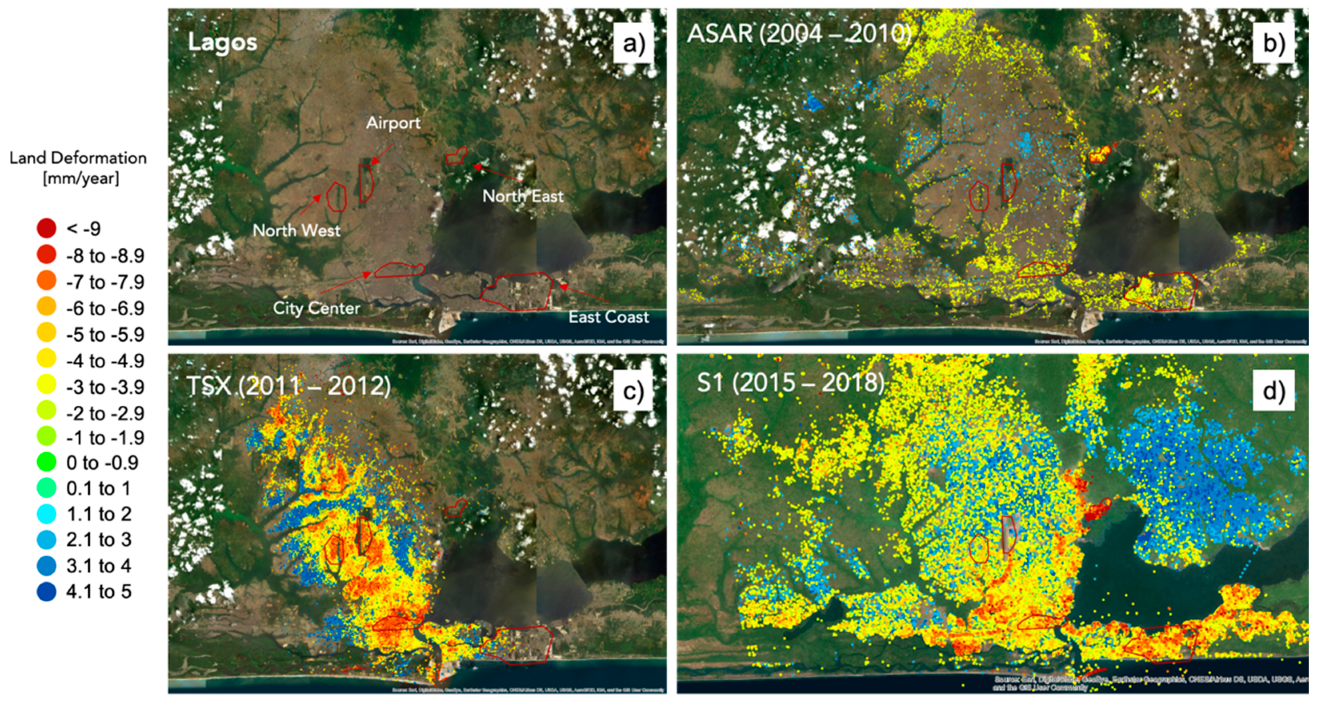
2.1.1. Lagos, Nigeria

Lagos is Nigeria’s largest city and busiest industrial and commercial center, built over a network of wetlands, swamps, creeks and islands around a lagoon and sitting an average of 1.5 m above sea level. The urban area is rapidly growing, estimated to have surpassed Cairo as the most populated city in Africa. The city’s more than 20 million inhabitants live in densely populated neighborhoods averaging over 20,000 persons per square kilometer [53]. Urban sprawl into the wetlands has been unplanned and today about two-thirds of the city’s population lives in vulnerable informal settlements with limited access to basic infrastructure. These residents face inadequate and absent sewage, drainage and water systems and lack the capacity to manage or maintain existing networks. Water access is unregulated and many households have sunk their own boreholes to tap into Lagos’s high groundwater table [53,54]. Flooding is pervasive during the rainy season (May to July and September to October), with climate change expected to increase annual rainfall and subsequent flood events for the city. Lagos also faces periodic storm surge events, which will increase in magnitude and frequency as tropical storms intensify [53]. Land reclamation and urban development have destabilized soils in key areas of the coast and north of the city. Around Lagos Lagoon and the floodplains of the Ogun River, sand filling extends real estate for housing developments. These new plots are built about 2 m above sea level and are vulnerable to rising sea level as a result of climate change. Lagos State has made efforts to reinforce Lagos’s key beaches. However, urban development is growing faster than urban planning can regulate. Sand mining, river damming and obstruction and vegetation destruction are also linked to Lagos’s quickly eroding shores [55,56].

2.1.2. Banjul, the Gambia
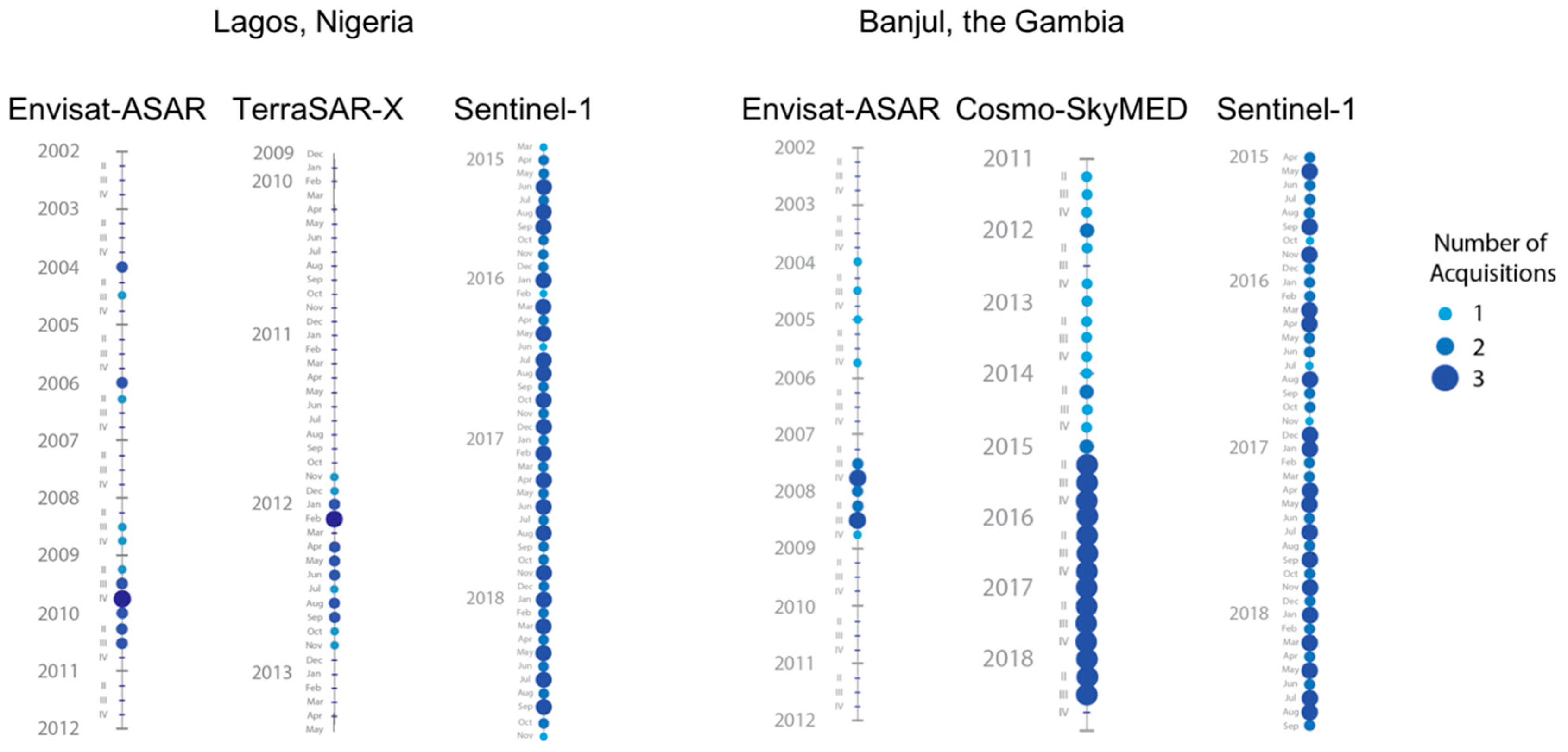
About one quarter of the Gambia’s total population lives in the greater Banjul area, which includes the cities of Banjul and Serrekunda and the municipality of Kanifing. Banjul city rests on a low-lying spit of coastal land at the mouth of the Gambia River, which, with anthropogenic factors such as unplanned urban expansion and deforestation, leaves its inhabitants vulnerable to climate-related hazards [57]. These areas have expanded without adequate stormwater management and drainage infrastructure and suffer heavy losses of life and property during annual rains and storms [58]. Flash floods and stormwater runoff are devastating to the urban coast, affecting 40,000 people every year [59]. Improper urban planning and management increase Banjul’s susceptibility to flood and wind. Additionally, land use zoning is ignored and housing construction and deforestation in flood-prone areas along the riverbank contribute to flood-related mortality and property damage. These unplanned settlements are expected to increase as urban populations grow. Many families must repair their houses annually or move to temporary locations following storms. A rise in sea level of 1 m would devastate greater Banjul, submerging over 90 square kilometers of land in the coastal zone and inundating the capital and its port [1,60]. A sea level rise of this magnitude would increase salinity levels along the river and in groundwater sources, diminishing freshwater supplies from coastal aquifers [61].

2.2. Data Used

There are several satellites with a SAR sensor on board and therefore acquiring suitable data for InSAR. Table 2 gives an overview of past and currently operational SAR missions. The main disadvantage of old missions, such as the European Space Agency’s ERS and Envisat, is the sparse acquisition of images, which limits the applicability of InSAR methodologies. Another limitation is the geometry of acquisition. For example, the Italian Space Agency’s CSK [62] is a constellation providing numerous images but with the limitation that on certain occasions the satellite is tilted to fulfill users’ requests or to respond to emergencies. InSAR cannot be applied to images acquired with different geometry, therefore the CSK archive cannot always be fully exploited for this purpose. However, the catalogue is very rich in InSAR time series for many of the cities analyzed in this study and it can be a very useful instrument to perform in-depth analysis.
S1 represents a revolution in InSAR since it provides very frequent acquisitions (6-day repeating cycle) with a stable acquisition geometry, an ideal scenario for InSAR analysis. Moreover, S1 data are easily and freely accessible through the Copernicus Science Hub [16].
In the analysis presented here, we made use of Envisat-ASAR data for monitoring land deformation from 2002 to 2010 and S1 from 2015 to today. Both ASAR and S1 data have a resolution of ~20 m, while the swath is about 100 km for ASAR and 250 km for S1.
Concerning the two case studies presented, for Lagos we were also able to access the TSX dataset and for Banjul we had access to CSK data. This allowed us to perform a higher-resolution analysis, given the 3 m resolution of these products.
Figure 2 shows the distribution of data available for the 2 case studies relative to the different sensors employed, while Table 3 provides a summary of details for the datasets employed.
It is clearly evident that the S1 and CSK archives allow for a more continuous analysis, given the homogeneous distribution of data throughout the whole time series, with the difference that CSK is not a freely accessible dataset. Regarding CSK data, there were more scenes available compared to the one reported. We could access only these images due to a free quota limit.

2.3. PSI Analysis by Means of SNAP and StaMPS

In PSI, among the available (n+1) images, one is selected as the master image. Interferograms are formed between the master and the n available slaves acquired on different dates. Each one is characterized by a certain perpendicular baseline, that is, the perpendicular distance between the 2 satellite positions. Knowing the precise position of the satellite on the 2 acquisition dates allows us to subtract from the interferogram phase the components related to the perpendicular baseline (flat earth and topographic components).
In an urban environment, manmade structures appear as persistent scatterers (PSs), since they reflect most of the energy sent by the SAR directly backwards or in a double-bounce mechanism (i.e., from the ground to a perpendicular structure and back to the sensor).
In PSI, the deformation phase is separated from the atmospheric phase and noise by filtering in time and space. In fact, deformation is correlated in time, while the effects of atmosphere are correlated in space but not in time (i.e., they are recognizable in one single interferogram but they are not correlated with other interferograms since the atmosphere changes randomly from one date to another). Finally, noise is uncorrelated in space and time.
PSI can associate deformation to a specific scatterer, allowing very high-resolution monitoring of infrastructures.
As shown in Figure 3, the first step was to create a subset of the n available S1 images. S1 images were divided into 3 sub-swaths. In most of the cases, the city of interest was contained in a single sub-swath. Each sub-swath is composed of several bursts (longitudinal portion of the image). Therefore, to create the subset, we selected the sub-swath containing the area of interest and the bursts covering exactly the area of interest [25]. This allowed us to reduce the size of data and speed up the processing. The second step was to compute individual interferograms, combining the master image with the remaining n slave images. Subset and interferogram computation was performed using SNAP open source software [63]. The stack of n individual interferograms was given as input for the PSI analysis (third step), where PSs are identified and analyzed. This step was performed using the StaMPS open source toolbox [46,64] for Matlab®. The toolbox gives as output the map of mean velocity of deformation for all the PSs in the area of analysis, as well as their deformation on each date of observation and the mean standard deviation of the velocity of deformation throughout the whole time series. Additionally, for the atmospheric phase removal of the data, we employed the Toolbox for Reducing Atmospheric InSAR Noise (TRAIN) [65] and applied the linear approach (phase versus elevation).
To automate the process of interferogram formation, we developed a set of scripts called “snap2stamps,” which, based on the setting of a few parameters (sub-swath of S1 images to be processed, bounding box of the area of interest, path to the data folder, path and name of the master image, parameters regarding the computational resources to employ, etc.), automatically compute interferograms. These scripts are Python wrappers that employ SNAP as the InSAR processor and provide output compatible with StaMPS to perform PSI analysis. Such sets of scripts are available as open source [14]. The last unofficial version can be found on the GitHub repository [66].
The overall analysis was composed of 3 main workflows: (i) single master interferogram processing using SNAP, (ii) PSI processing using StaMPS and (iii) results analysis in a geographic information system (GIS) environment.
In workflow (i), the first step is to identify the master image using the “InSAR Stack Overview” command of SNAP. After that, the area of interest (AOI) inside the master image has to be identified and used to split the master image using the SNAP graphical user interface (GUI). In this way, a single image swath is selected along with the bursts needed to cover the AOI. This operation reduces data volume and optimizes processing time and resources. At this point, we can make use of the snap2stamps scripts to prepare the slave images and compute the interferograms. The scripts sort the slave images by acquisition date, place them in subsets based on the master extent, co-register each of them with the master image and compute the interferograms, which are finally exported for analysis in StaMPS. For details about these operations, refer to the documentation of the snap2stamps package [14].
In workflow (ii), the first step is to prepare the exported data to be analyzed in StaMPS using the mt_prep_snap script. Next, within Matlab®, StaMPS can be run from steps 1 to 7 as described in the StaMPS user manual [64] using TRAIN for the APS mitigation using the aps_linear approach to perform the PS analysis. The output is a map containing points bearing the land deformation values throughout the time series.
In workflow (iii) (Figure 4), the land deformation maps are loaded in a GIS, where points showing deformation greater than or equal to ±2 mm/year are selected and analyzed. For each area showing interesting behavior (AOI), 3 plots are produced: (i) a plot showing the distribution of velocity of deformation values for all the analyzed points, (ii) a plot showing the distribution of the standard deviation values of the velocity of deformation for all the analyzed points and (iii) a plot showing the deformation trend of each point measured at each time step of the time series. The plots allow us to understand the average behavior of the points inside the AOI. The first plot indicates the average deformation (subsidence, uplift or stability), the second indicates the stability of velocity of deformation values and the third shows the trend of deformation along the time series.
The data processing for all the cities analyzed within the CityCORE project was performed within the virtual environment provided by the ESA Research Support System (ESA RSS) CloudToolbox service [67], with 8 vCPUs, 52 GB RAM and 4 TB disk space available.

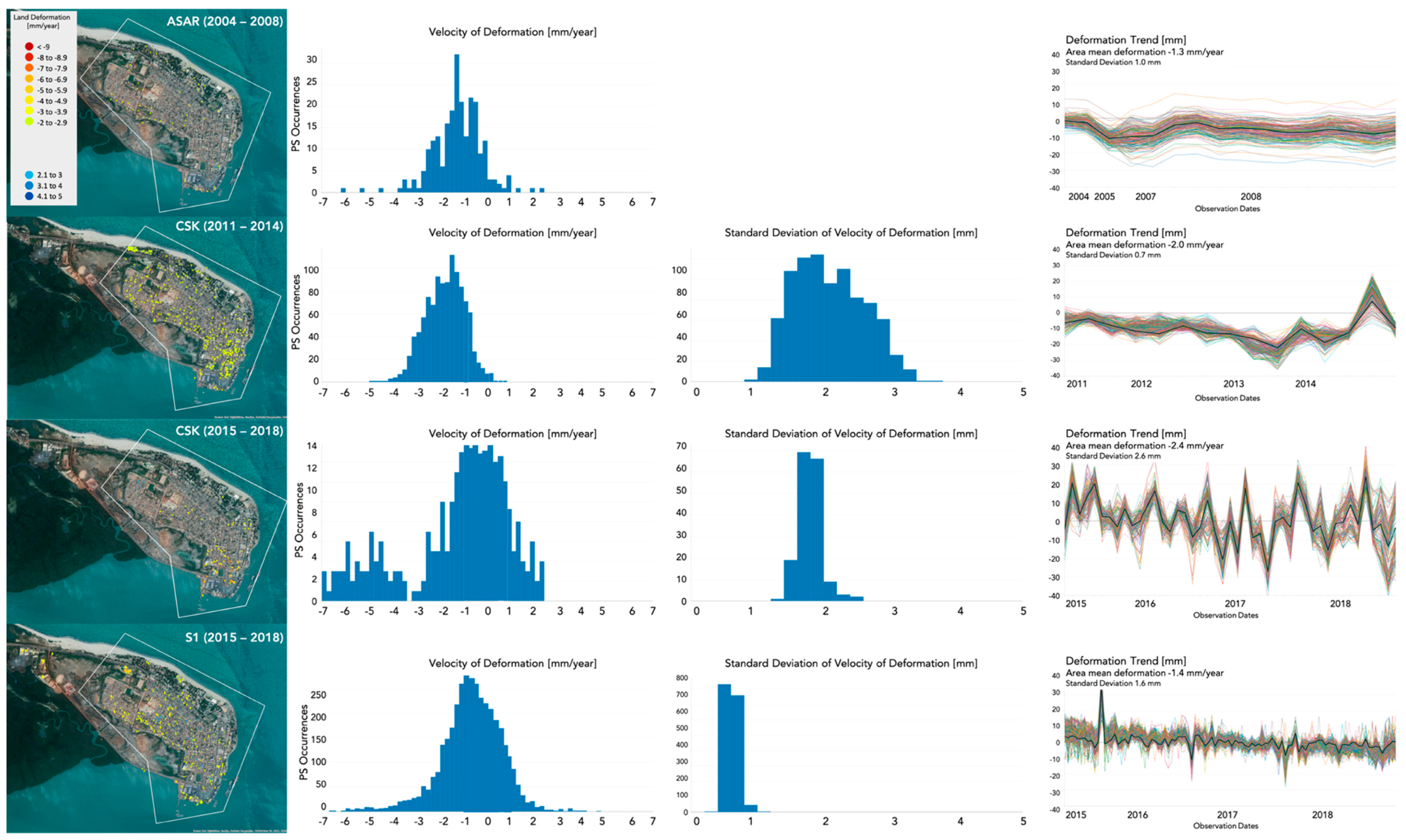
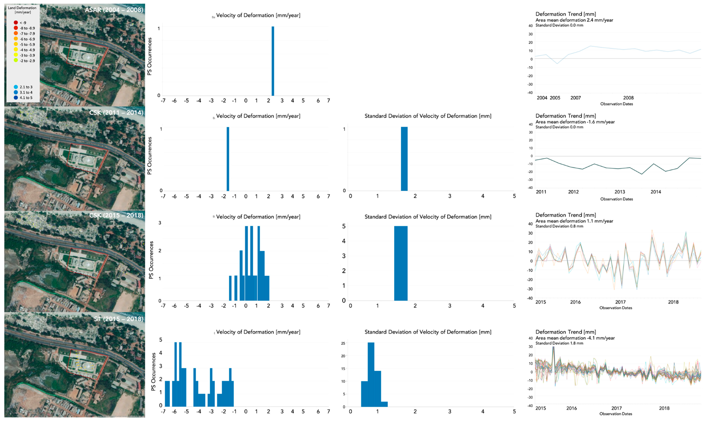
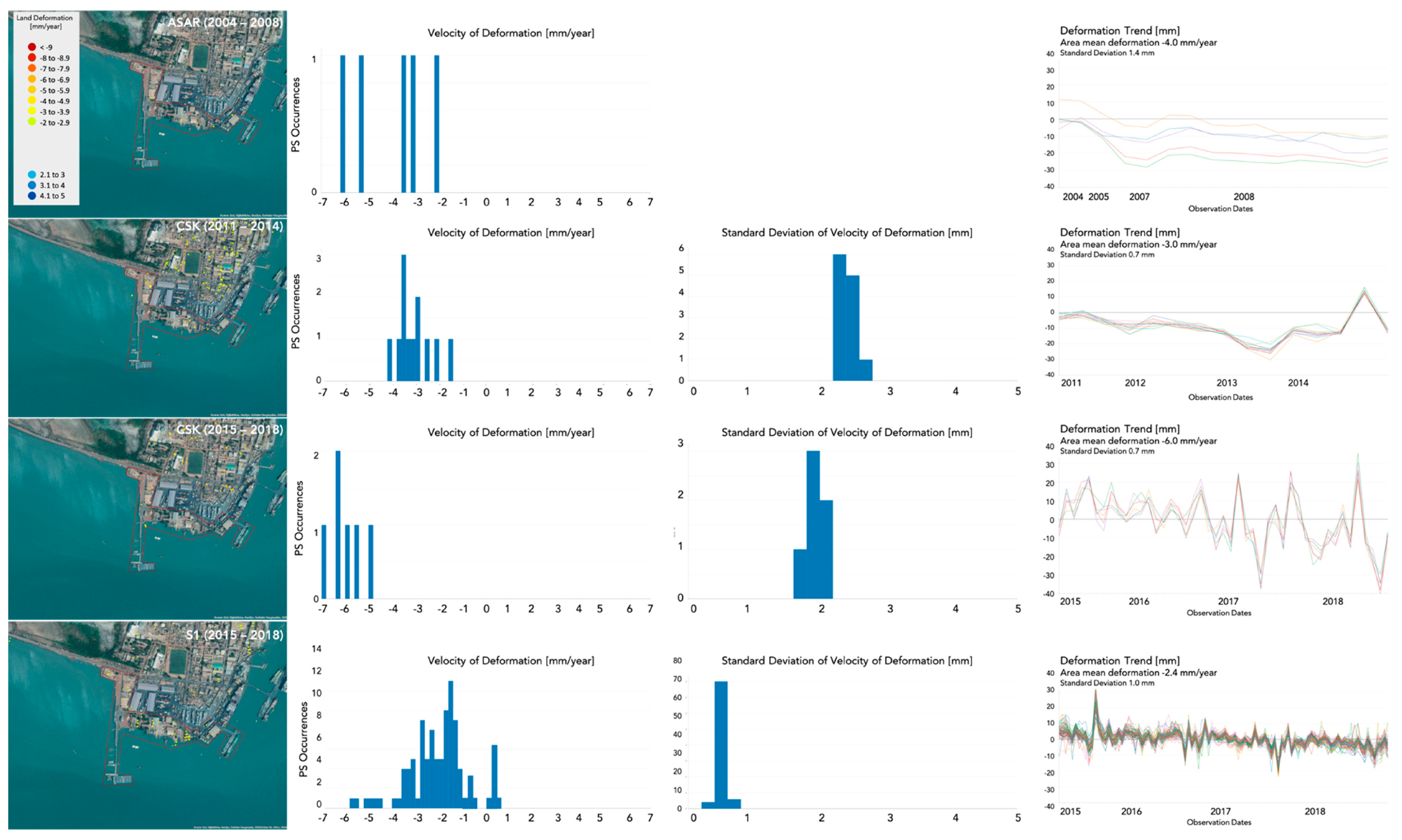
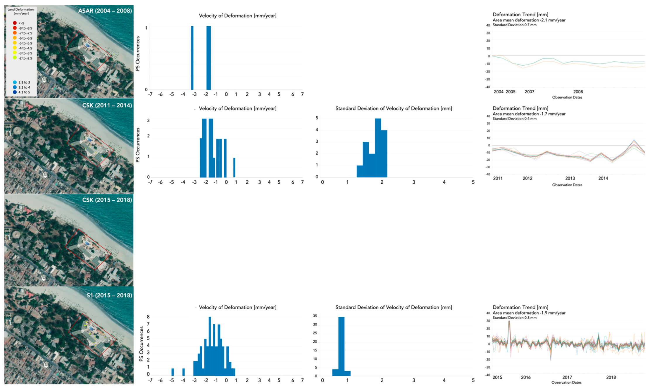
3. Results and Discussion
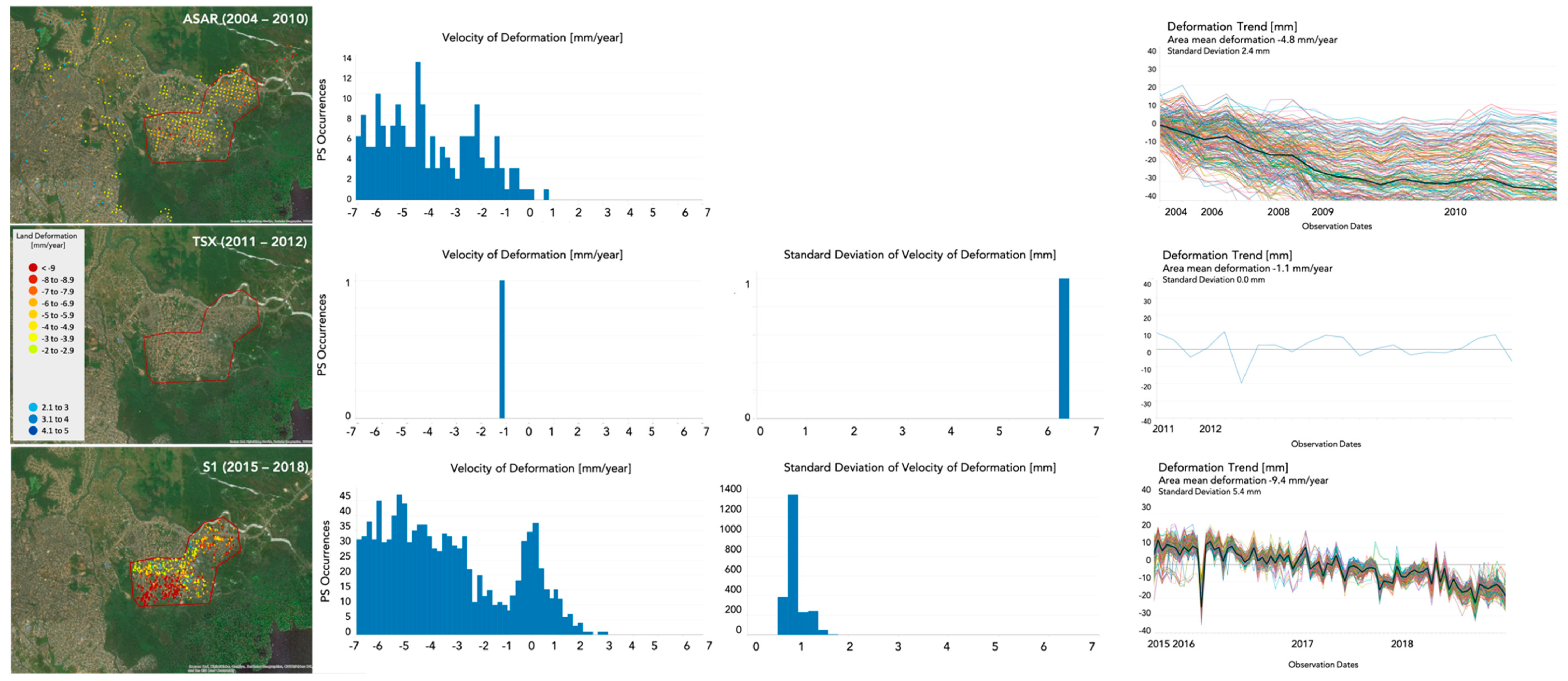
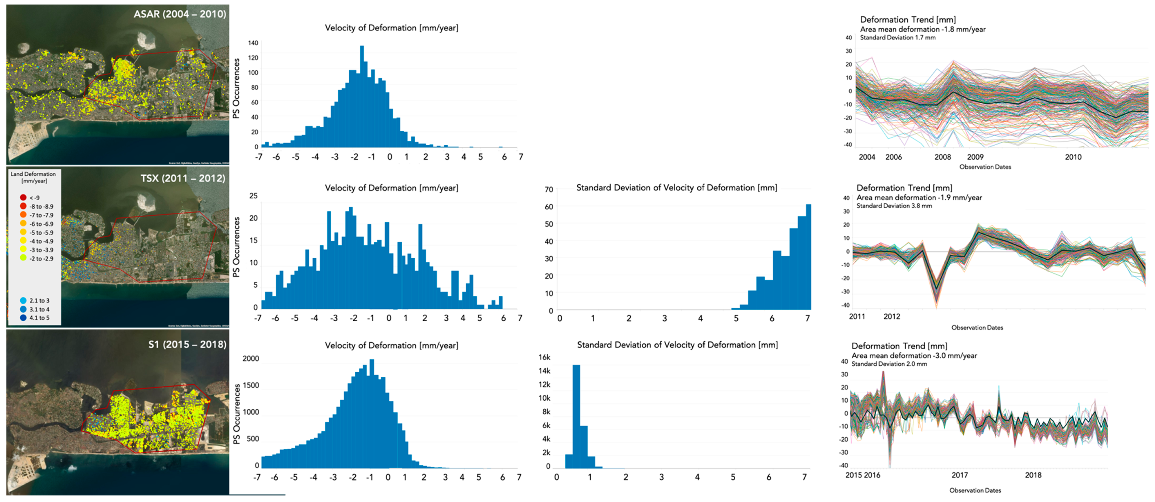
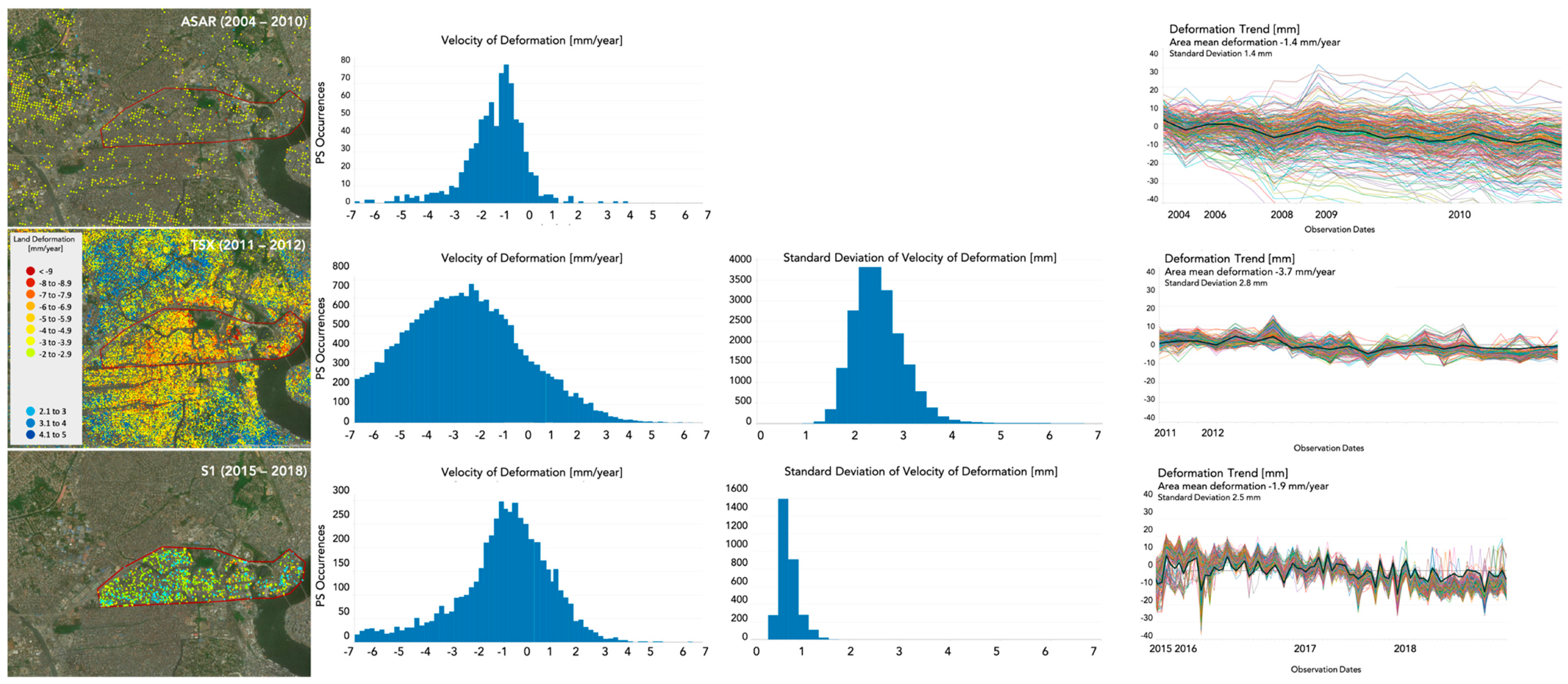
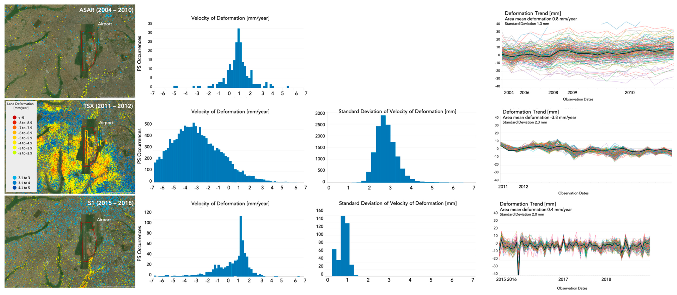
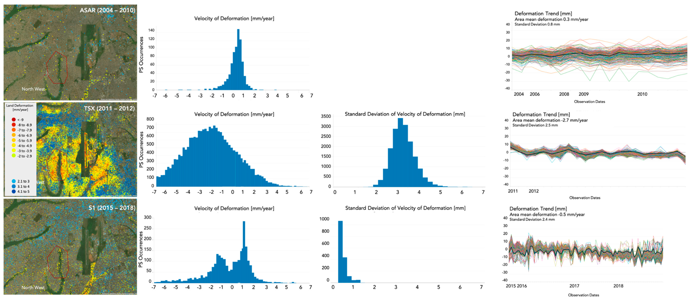
For both case studies, we present the results obtained using Envisat-ASAR and S1 data. In addition, we also made use of TSX data for Lagos and CSK data for Banjul, both at 3 m resolution. The results show maps of velocity of land deformation in mm/year during the period of observation for the PSs identified in each time series. The velocity of deformation can be negative, meaning land subsidence or positive, meaning land uplift. The deformation values refer to the line of sight (LOS) of the satellite and can have both a vertical and a horizontal component. Given that the incidence angle is less than 45° for all the acquisitions employed in the study, it is more likely that the dominant component is the vertical one. To discriminate the two components, we would need field measurements, not available at this stage or acquisitions from a different orbit, not available for every case study and not analyzed at this stage of the research. However, a different incidence angle would influence the magnitude of the detected displacement in LOS; specifically, the lower the incidence angle, the higher the measured LOS, given the same vertical displacement. To analyze our results, we had to bear in mind the different incidence angles of the datasets. In particular, ASAR has an average incidence angle of about 20°, S1 of about 38°, CSK of about 27° and TSX of about 40°. Therefore, taking S1 results as a reference, for the same vertical displacement, ASAR would show a displacement about 15% higher, CSK 10% higher and TSX 5% lower.
With the aim of highlighting significant deformations, the results were filtered, excluding points indicating mean velocity of land deformation between −2 and 2 mm/year, values considered as noise. This interval was chosen based on values found in the literature and on the characteristics of the data employed in the study. In fact, Sabater et al. [68] compared the results of ground deformation measurements obtained with different sensors. They found that using C band (5.6 cm), used by ASAR and S-1, the precision is 1.1 mm, while using X band (3.1 cm), used by TSX and CSK, the precision is 0.6 mm. This justified the interval chosen, which was suitable for all the data employed. Moreover, movements below 2 mm/year can be considered as not critical within the deformation of a city.
At the same time, we had to bear in mind that these differences in terms of precision must be considered when analyzing the results [69]. Finally, the sensitivity to surface change, higher for X band, also must be considered in analyzing the results.
For each case study, five AOIs were selected and analyzed in detail. For each AOI, we produced three plots: (i) the distribution of the values of velocity of deformation, (ii) the distribution of the values of standard deviation of the velocity of deformation and (iii) the trend of deformation for each point analyzed through the whole time series, which shows also the overall mean velocity of deformation, that is, the mean of the mean velocity of deformation of each PS within the AOI and its standard deviation, that is, the standard deviation computed on the mean velocity of deformation of each PS within the AOI. The plots allow us to understand the magnitude of the deformation (velocity), its reliability (standard deviation) and its evolution over time (trend). In the case of ASAR data, the standard deviation was not computed (plot ii)).

3.1. Lagos, Nigeria

Figure 5 shows the results obtained for Lagos, Nigeria, using ASAR data for the period 2004–2010, TSX data for the period 2009–2012 and S1 data for the period 2015–2018. The points showing deformation between −2 and 2 mm/year were filtered out of the image as they are considered noise, as explained at the beginning of the section. Five areas of interests (AOIs) were considered for detailed analysis: northeast Lagos, east coast, city center, airport and northwest.
Regarding the datasets (Figure 2), the distribution of the 20 ASAR acquisitions is suboptimal, with sparse acquisitions from the beginning of 2004 to the end of 2010. Most of the acquisitions (12) are concentrated between the second quarter of 2009 and the third quarter of 2010. Instead, the distribution of the 98 S1 images is optimal, with acquisitions very well distributed from April 2015 to November 2018. Finally, the 23 TSX images are optimally distributed from November 2011 to November 2012.
The results derived from ASAR data (Figure 5b) show that most of the city was stable for that time period, with only some areas of significant subsidence (from −2 to −5 mm/year) in the northern part of the city, a small area on the east side and some areas on the south side close to the coast. Given the distribution of ASAR images, we can attribute this deformation to the two years between mid-2008 and mid-2010. Despite a lower sensitivity to displacement of C band, ASAR shows points covering the whole city with a magnitude within the ±2 mm/year noise threshold, indicating a stable land surface.
The analysis obtained with TSX data (Figure 5c) shows significant differences from previous results. If the southern coast shows similar behavior, the central-northern part of the city shows strong signals of land deformation not detected by ASAR in previous years. Moreover, the northern and eastern sides of the city, where we detected subsidence using ASAR data, do not appear in the map, indicating stable behavior during the period of analysis. As will be described in more detail in the following, TSX results are affected by a strong fluctuation of values along the time series and the mean velocity of deformation is affected by a high standard deviation (more than 2 mm/year, in many cases more than 5 mm/year). This is partly due to a higher sensitivity to displacements of X band.
The analysis based on S1 data (Figure 5d) shows similarities with ASAR and TSX results, in particular on the northern and southern sides of the city, where we can notice subsidence consistent with that detected by ASAR and TSX.
To better understand the results, five AOIs (Figure 5a) were selected and analyzed in detail, based on the land deformation signal they showed and their importance within the city.
The analysis carried out for the northeast AOI is shown in Figure 6. This area (Erunkan) has been developed in the past 15 years on reclaimed land. Therefore, many buildings are of new construction, with many still under development as shown by Google Earth Street View. The results obtained with the three datasets all show land subsidence but with some differences. Using ASAR data, we detected PSs showing land subsidence in many cases greater than 5 mm/year, with an overall subsidence of 4.8 mm/year (standard deviation of 2.4 mm). The subsidence is shown to have a constant rate throughout the time series. Most of the points are on the north side of the AOI. This is due to the development of the neighborhood, which occurred toward the south side after 2010 and is impossible to capture by ASAR. Using TSX data, we were able to obtain only one PS, which is not enough to infer information about the area. Using S1, we obtained PS points in the entire AOI. Especially on the south side, we can observe a strong signal of land deformation. Most of the PSs show subsidence with magnitude greater than 3 mm/year and for hundreds of PSs greater than 5 mm/year. These values appear to be precise given the low value of the standard deviation (the majority below 1 mm/year). The trendline plot, despite some fluctuations, shows land subsidence with a constant rate, with a mean velocity of 9.4 mm/year (standard deviation of 5.4 mm/year among all the analyzed points). The observed subsidence is most likely due to compaction of the land under the weight of the new buildings.
The analysis carried out for the east coast AOI is shown in Figure 7. This area (Lekki) went through significant development in the past 10 years, with land reclamation and new construction (see Google Earth Street View). Using ASAR data, we detected hundreds of PSs showing land subsidence with a distribution of values centered around −2 mm/year. The overall subsidence is 1.8 mm/year (standard deviation of 2.4 mm). The subsidence appears to have a constant rate throughout the time series. Most of the points are on the west side of the AOI. This is due to the development of the neighborhood, which occurred toward the east side after 2010 and is impossible to capture by ASAR. Using TSX, we obtained tens of PSs mainly on the west side of the AOI. They also indicate a general subsiding trend (1.9 mm/year mean subsidence) but with more fluctuations throughout the time series leading to an important standard deviation value of 3.8 mm. Despite being consistent with the other results, these do not seem to be reliable. Using S1, we obtained thousands of PSs in the entire AOI. Most of these PSs show subsidence with a magnitude greater than 2 mm/year and for several thousands of them, greater than 5 mm/year. These values appear to be reliable given the low value of the standard deviation (the majority below 1 mm/year). The trendline plot, despite some fluctuations, shows constant land subsidence, with a mean velocity of 3.0 mm/year (standard deviation of 2.0 mm/year among all the analyzed points).
The analysis carried out for the city center AOI is shown in Figure 8. This area (Ijora) appears to be quite stable in terms of development in the past 15 years. Using ASAR data, we detected tens of PSs (few compared to other datasets) showing a slight trend of land subsidence with a distribution of values centered around −1 mm/year. The overall subsidence is 1.4 mm/year (standard deviation of 1.4 mm). The subsidence shows a constant rate throughout the time series. Using TSX, we obtained thousands of PSs indicating a general subsiding trend (3.7 mm/year mean subsidence) but with fluctuations throughout the time series (standard deviation of 2.8 mm). Using S1, we obtained thousands of PSs showing subsidence with magnitude greater than 1 mm/year, for several hundreds of them greater than 5 mm/year. These values appear to be reliable given the low value of the standard deviation (the majority below 1 mm/year). The trendline plot, despite some fluctuations, shows land subsidence with a constant rate, with a mean velocity of 1.9 mm/year (standard deviation) of 2.5 mm/year among all the analyzed points).
The analysis carried out for the airport AOI is shown in Figure 9. The results obtained with the three datasets show varying behavior, most probably because different periods of analysis experienced different deformation patterns. Using both ASAR and S1 data, we detected only a few PSs, most of them outside of the airstrip. In both cases, the distribution of values of velocity of deformation is centered around an uplift of 1 mm/year, for S1 with standard deviation below 1 mm/year. The trendlines show a mean uplift of 0.8 mm/year for ASAR and 0.4 mm/year for S1. However, the standard deviations of this mean uplift among all the analyzed points are 1.3 mm/year for ASAR and 2 mm/year for S1, indicating considerable variability.
On the contrary, using TSX, we detected thousands of PSs, many falling within the main airport strip, showing a strong signal of subsidence. Most of the PSs show subsidence with magnitude greater than 4 mm/year, for hundreds of PS greater than 6 mm/year. These values appear to be not very precise given a standard deviation centered around 2.8 mm/year. The trendline plot, despite considerable fluctuations, shows land subsidence with a constant rate, with a mean velocity of 3.8 mm/year (standard deviation of 2.3 mm/year among all the analyzed points).
The analysis carried out for the northwest AOI is shown in Figure 10. This area (Egbe and Ejigbo) does not show any significant change in the past 15 years. The results, as in the previous case, show varying behavior, with ASAR and S1 detecting few PSs, with a predominant slight uplift in the case of ASAR (0.3 mm/year mean deformation) and a predominant land subsidence in the case of S1 (−0.5 mm/year mean deformation) but with 2.4 mm/year standard deviation among the mean deformation of all the PSs. Using TSX, we detected thousands of points showing a strong signal of subsidence, with a distribution peak between −2 and −3 mm/year, hundreds of points with deformation greater than −5 mm/year. The distribution of the standard deviation in this case is centered around 3 mm, indicating some uncertainty in these measurements. This is also confirmed by the trendlines, showing a mean deformation of −2.7 mm/year with 2.5 mm standard deviation.
By looking at these results, we can immediately notice how higher resolution can bring more details. In fact, TSX is able to detect a higher density of PSs compared to S1 and ASAR, allowing the detection of deformation at building scale in case of good coherence throughout the whole time series. However, the big advantage brought by S1 is the frequency of acquisition, which increases the ability to detect PSs and the precision of measuring their velocity of deformation. This is evident by the distribution of the standard deviation values. On the contrary, ASAR, which allowed the analysis of land deformation in the past, has coarser resolution and few images not continuously acquired and not well distributed throughout its acquisition life. TSX, which has the advantage of higher resolution but is not freely accessible, also has a longer and discontinuous frequency of observation, which strongly affects the InSAR analysis.
The higher resolution of TSX allows for increased details in the analysis, as is evident in the city center and airport AOIs but seems to introduce more uncertainty to the measurements, as shown by the fluctuations on the trendlines. This may be due to the characteristics of the area, made up of unstable buildings and by the X band signal that can be strongly affected by the atmosphere, quite important in this area of the world.
S1 data appear to be a very good compromise given the level of detail they can provide and the stability of the measurements and they are freely accessible.

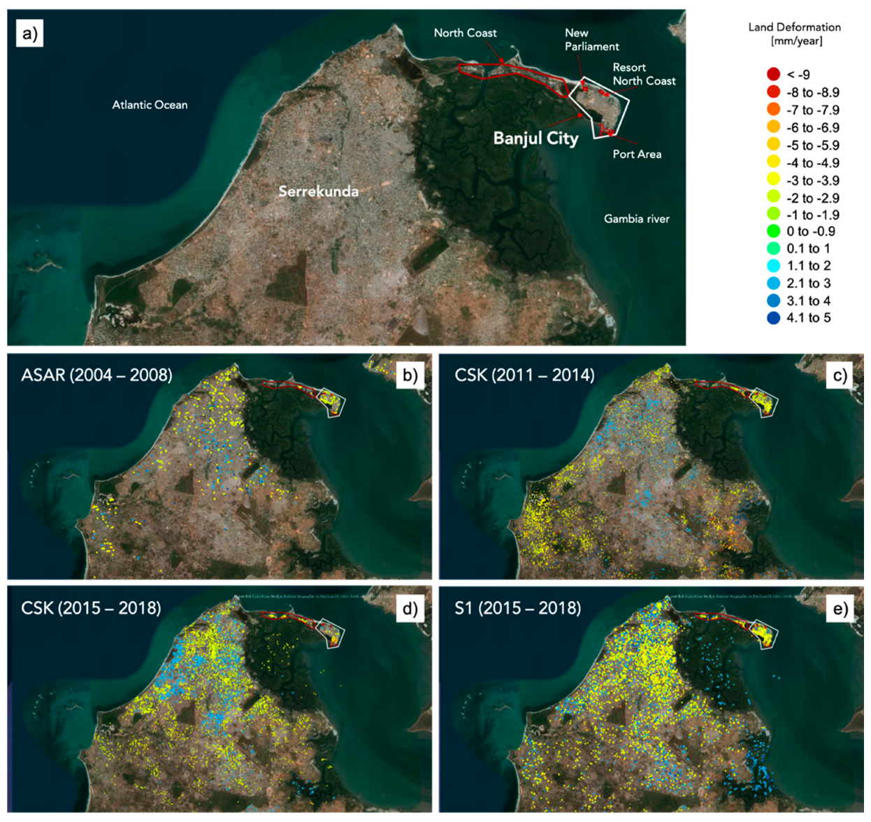
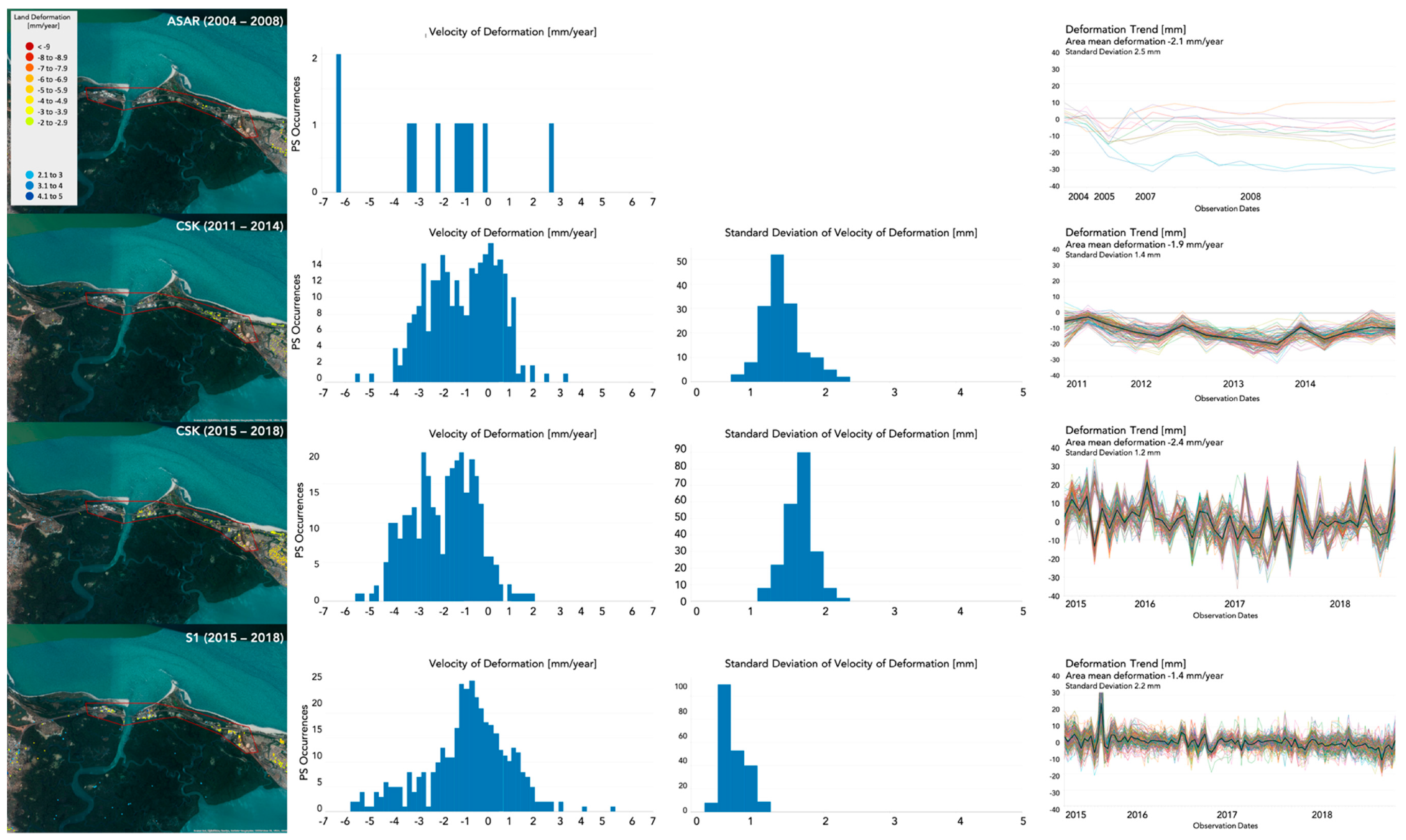
3.2. Banjul, the Gambia

Figure 11 shows the results obtained for Banjul, the Gambia, in particular those obtained with ASAR data for the period 2004–2008, CSK data for the periods 2011–2014 and 2015–2018 and S1 data for the period 2015–2018. The points showing deformation between −2 and 2 mm/year were filtered out of the image as they are considered noise. Five AOIs were considered for detailed analysis: Banjul city, new Parliament, port area, resort north coast and north coast.
Regarding the datasets (Figure 2), the distribution of the 17 ASAR acquisitions is suboptimal, with sparse acquisitions (4 images) from the beginning of 2004 to the end of 2005. Most of the acquisitions (13) are concentrated between the third quarter of 2007 and the fourth quarter of 2008. On the other hand, the distribution of the 100 S1 images is optimal, with acquisitions very well distributed from April 2015 to September 2018. Concerning the CSK data, the availability of acquisitions in the catalogue was optimal from 2011 until the end of 2018. However, given the limited number of scenes we could obtain, we selected a total of 60 images. Given the changes that occurred in the city of Banjul in between 2011 and 2018 (for example, construction of the new national assembly building), to capture deformations of the new constructions, we decided to analyze the images in two groups: 15 images covering the period May 2011 to December 2014 with an average distribution of 1 image per quartile and 45 images covering the period January 2015 to September 2018 with an average distribution of 1 image per month.
The results derived from ASAR data (Figure 11b) show that the majority of the city is stable, with only some areas of significant subsidence (from −2 to −4 mm/year) in the old city of Banjul. Given the distribution of ASAR images, we can attribute this deformation mainly to the years 2007 and 2008.
The analysis performed with CSK data for 2011–2014 (Figure 11c) shows similar results, highlighting some interesting land subsidence in the old city of Banjul (−2 to −4 mm/year) with a higher density of PSs. This is also confirmed by the analysis carried out using CSK data for 2015–2018 (Figure 11d). In this case we obtained a lower density of PSs but some of them indicated stronger land subsidence (<−4 mm/year). As for TSX data over Lagos, shown in the previous section, the results obtained using CSK data are also affected by a strong fluctuation of values along the time series and the mean velocity of deformation is affected by a high standard deviation (more than 2 mm/year). Given that CSK also uses X band, these stronger fluctuations can be linked to the higher sensitivity of X band to displacement.
Finally, the analysis performed with S1 data (Figure 11e) shows a scattered presence of subsiding points in the Serrekunda area and, once again, a concentration of points in the old city, indicating subsidence (mainly between −1 and −3 mm/year).
To better understand the results, five AOIs (Figure 11a) were selected and analyzed in detail, based on the land deformation signals they showed and their importance within the city.
The analysis carried out for the Banjul city AOI is shown in Figure 12. This old area did not experience much development in recent years, with the exception of few new constructions. The area is basically a sand island on the mouth of the Gambia River, which makes it an unstable environment in terms of land deformation. The results obtained with the four datasets all show land subsidence with similar magnitude. The densities of PSs are different, with S1 and CSK (2011–2014) detecting several hundreds and ASAR and CSK (2015–2018) just over 100. Their distribution over the city is different depending on the dataset used, therefore depending on the period of analysis. This will be clearer in the following, where we analyze subsets of this area.
Using ASAR data, we detected PSs showing land subsidence mainly between 0 and −3 mm/year, with an overall subsidence of 1.3 mm/year (standard deviation of 1 mm). The subsidence shows a constant rate throughout the time series.
The results derived from CSK (2011–2014) show very similar subsidence supported by many more PSs, with an overall magnitude of 2 mm/year (standard deviation of 0.7 mm). However, the PSs show a high value of standard deviation, with a distribution centered at 2 mm but with tens of PSs reaching 3 mm.
The results obtained from CSK (2015–2018) exhibit fewer PSs (about 100 in total) with a similar subsidence magnitude. However, in this case, we found PSs showing a stronger subsidence signal (<−4 mm/year). The analysis shows an overall subsidence of 2.4 mm/year but with a much stronger fluctuation of values (standard deviation of 2.6 mm). Despite a continuous trend of land subsidence recognized in the time series, the fluctuation of the values makes this analysis less reliable.
Using S1, we obtained several hundreds of PSs in the entire AOI, some detecting a strong signal of land deformation (<−4 mm/year). Most of the PSs show subsidence in the range of −1 and −3 mm/year. These values appear to be very precise given the low value of the standard deviation (the majority below 1 mm/year). The trendline plot, despite some fluctuations, shows land subsidence with a constant rate, with a mean velocity of 1.4 mm/year (standard deviation of 1.6 mm among all the analyzed points).
The analysis carried out for the new Parliament AOI is shown in Figure 13. Construction of this new building ended in 2014, which is why, using the ASAR and CSK (2011–2014) datasets, we were able to find only one PS, which of course does not bring any information about the land deformation of this area. We were expecting to find many PSs using the CSK (2015–2018) dataset, which detected only 10 PSs that did not fall within the main building itself. The overall deformation reported is a land uplift of 1.1 mm/year (standard deviation of 0.8 mm). However, the distribution of standard deviation of the velocity of deformation values is between 1.5 and 2 mm, making these measurements unreliable. Using S1 data, we detected about 50 PSs falling over the new national assembly building. In this case, the land subsidence trend is clear, with the distribution of velocity of deformation showing that all PSs have a land deformation lower than –1 mm/year. The distribution of the standard deviation values is centered around 1 mm, indicating a reliable measurement. The trendlines show clear land deformation, with a constant rate throughout the time series, with an overall mean land subsidence of 4.1 mm/year (standard deviation of 1.8 mm among all the analyzed points). The observed subsidence is most likely due to compaction of the land under the weight of the new building or the settlement of the structure itself.
The analysis carried out for the port area AOI is shown in Figure 14. This area experienced some development in the past 15 years, with extensions of existing piers and construction of buildings. The results obtained with the three datasets all show a trend of land subsidence. Using ASAR data, we detected only five PSs but they show a clear land subsidence trend, with an overall mean velocity of deformation of −4 mm/year (standard deviation of 1.4 mm among all the analyzed points). The subsidence appears to have a constant rate throughout the time series but the very low PS density cannot tell us much about the deformation in this area. Using CSK (2011–2014) data, we obtained 12 PSs all showing land subsidence, mainly concentrated between −3 and −4 mm/year. However, the distribution of standard deviation values is centered between 2 and 3 mm, indicating considerable variability. The trendlines show a constant trend of subsidence throughout the time series, with the exception of the acquisitions in 2014, which show high variability. The overall mean land deformation is −3 mm/year (standard deviation of 0.7 mm among all the analyzed points). Similarly, using CSK (2015–2018) data, we detected only six PSs, showing land subsidence between −5 and −7 mm/year, with a distribution of standard deviation values centered at 2 mm. The trendlines show a constant trend of subsidence throughout the time series, with overall mean land deformation of −6 mm/year (standard deviation of 0.7 mm among all the analyzed points). The few detected PSs, unfortunately, cannot tell much about the entire area. Instead, using S1, we detected about 100 PSs showing land subsidence between −1 and −6 mm/year, with distribution of standard deviation values centered at 0.5 mm, indicating very precise measurement. Despite some fluctuations, the trendlines show a clear land subsidence trend, which appears to intensify in the second half of the time series. The overall mean velocity of deformation is −2.4 mm/year (standard deviation of 1 mm among all the analyzed points).
The analysis carried out for the resort north coast AOI is shown in Figure 15. As in the case of AOI 2, this is a very small area and we were expecting few PSs. Using ASAR data, we detected only three PSs, showing subsidence between −1 and −3 mm/year. The trendlines show a constant rate of land subsidence with an overall mean velocity of deformation of −2.1 mm/year (standard deviation of 0.7 mm among all the analyzed points). Using CSK (2011–2014) data, we obtained 15 PSs, all showing land subsidence between −1 and −3 mm/year, with a distribution of standard deviation values centered at 2 mm. The trendlines show a constant trend of subsidence throughout the time series, with the exception of the acquisitions in 2014, which show high variability. The overall mean land deformation is −1.7 mm/year (standard deviation of 0.4 mm among all the analyzed points). Using CSK (2015–2018) data, we detected no PSs. Instead, using S1, we detected about 40 PSs showing land subsidence mainly between −1 and −3 mm/year, with distribution of standard deviation values centered at 0.8 mm, indicating very reliable measurement. Despite some fluctuations, the trendlines show a clear land subsidence trend. The overall mean velocity of deformation is −1.9 mm/year (standard deviation of 0.8 mm among all the analyzed points).
The analysis carried out for the north coast AOI is shown in Figure 16. Using ASAR data, we detected 10 PSs, showing subsidence between −1 and −3 mm/year. The trendlines show a constant rate of land subsidence between 2007 and 2008, with an overall mean velocity of deformation of −2.1 mm/year (standard deviation of 2.5 mm among all the analyzed points). Using CSK (2011–2014), we obtained more than 100 PSs showing mostly land subsidence between −1 and −4 mm/year, with a distribution of standard deviation values centered at 1.4 mm. The trendlines show a constant trend of subsidence throughout the time series, with the exception of the acquisitions in 2014, which show high variability. The overall mean land deformation is −1.9 mm/year (standard deviation of 1.4 mm among all the analyzed points). Also using CSK (2015–2018) data, we detected more than 100 PSs, with a land subsidence between −1 and −4 mm/year. The distribution of standard deviation values is centered at 1.6 mm. The trendlines show an overall trend of land subsidence characterized by strong fluctuations. The overall mean land deformation is −2.4 mm/year (standard deviation of 1.2 mm among all the analyzed points). Using S1 data, we detected more than 100 PSs showing a predominance of land subsidence mainly between −1 and −2 mm/year. The distribution of standard deviation values is centered at 0.5 mm, indicating very reliable measurement. Despite some fluctuations, the trendlines show a land subsidence trend with an overall mean velocity of deformation of −1.4 mm/year. The standard deviation is 2.2 mm among all the analyzed points, high as expected given the presence of many points indicating land uplift. As this area is a productive site, the land deformation exhibited in all four analyses makes it important for further monitoring.
The results show an overall agreement between the deformations measured employing different datasets. As in the case of Lagos, we notice that, in general, a higher resolution can lead to a higher density of PSs. However, the results based on CSK in some cases show a lower density of PSs. This is due to the instability of the structures (houses, building, shacks, etc.) or their roofs, characteristic of this region. As in the case of Lagos, weather conditions could also play a significant role in the precision of the measured deformation, being X band sensitive to the atmosphere. In general, for Banjul we can affirm that CSK data do not appear to be very reliable. In fact, the fluctuations of measurements in some cases are too big to trust the mean velocity of deformation. A combination of high resolution, short wavelength and unstable structure of the urban texture is most likely the cause of this low level of accuracy. However, TSX data, which is very similar to CSK, appeared to be more reliable than CSK data, considering that Lagos is not a completely different environment compared to Banjul. Probably the more developed condition of Lagos plays a role in the resulting PS density. The advantage of the CSK dataset compared to TSX is the wide and continuous availability of images from 2011 to today.
The lower density of PSs detected by ASAR data was expected due to the resolution of the data. In addition, the low frequency of observations in the first part of the time series (2004 to 2005) results in fluctuations in the deformation measured.
S1 in this case also appeared to have very reliable datasets, allowing us to obtain very precise measurements (characterized by low values of velocity of deformation standard deviation) and perform large-scale land deformation analyses.

4. Conclusions

In this paper, we presented a methodology for performing land deformation analysis based on the integrated use of SNAP and StaMPS and applied at large scale, employing a large amount of data and using different sensors. We presented the results for the city of Lagos, Nigeria, where we used ASAR, TSX and S1 data and Banjul, the Gambia, where we used ASAR, CSK and S1 data. The results showed hotspots of land deformation. While the analyses should be further investigated, particularly with field measurements, they are nevertheless of interest for local authorities and urban planners.
The methodology proved to be easy, detailed and reliable in obtaining InSAR time series analysis from a large amount of data, such as the long S1 time series and the high-resolution CSK and TSX time series. This allows moving toward a more accessible InSAR analysis. In fact, with this easy and semiautomatic methodology coupled with a free accessible dataset, such as the S1, transferring knowledge, especially to developing countries, becomes more feasible, allowing capacity to be built within the framework of a very complex technology.
Within the framework of the CityCORE Africa project, which aims to improve the resilience of selected coastal cities in sub-Saharan Africa, we were able to apply this methodology to 18 cities with the aim of highlighting possible critical land deformation hotspots. We employed about 1000 S1 images covering an area of about 20,000 km2.
In particular, S1 images are acquired with enough frequency and cover extensive enough areas to allow the analysis of fast-growing cities, such as the African cities analyzed in this study. The dataset is freely accessible and continuously updated thanks to the global systematic acquisition plan of the S1 mission, allowing constant monitoring of the areas of interest. The open access of the data, its wide area coverage and the frequency of observation allow hotspots of land deformation to be exposed at limited cost.
Despite not being freely accessible, high-resolution commercial SAR data are available over most of the selected cities and allow a detailed analysis (3 m resolution and more) of land deformation, such as the case of CSK data available from 2011.
The presented methodology shows various limitations. Some are purely related to the technology employed. For instance, precipitation and water content in the atmosphere can significantly affect the results, introducing disturbances in the radar signals, which influence the measured deformation and this introduces fluctuations in the measured deformation time series and uncertainty in the mean deformation value; a long time series of images can limit this source of error. The measured deformation is expressed in the direction of the line of sight of the SAR antenna, which is about 30° from the nadir and in order to derive its vertical and horizontal components, two compatible measurements should be available, one from an ascending and one from a descending orbit; this would increase the capacity needed in terms of computation and time of analysis and also cost in the case of commercial data. Despite the abundance of S1 data, in many cases SAR images are available only from a single orbit, especially when there is a need to go back in time, before the advent of S1. The resolution of older SAR data, such as Envisat-ASAR and the more recent S1 employed in this study, does not allow for precise analysis at building scale, for which commercial data at high resolution is needed, as shown in the case of Lagos by means of TSX data. The extensive lack of independent measurements, such as with Global Positioning System (GPS) data, does not allow for validation and calibration of the results, which is important for calibrating a precise model of deformation. This is especially true for African cities. However, developments in the field of smart sensors can allow automatic and low-cost monitoring of buildings and structures [69,70], which could be useful for integrated InSAR analysis.
Other limitations are connected to the dataset employed. The use of S1 data was shown to be particularly effective; however, in many cases data were available only for one or two years. This is a short time frame for a precise analysis; older data archives such as those of Envisat-ASAR and ERS-1 and -2 may cover longer time periods but the data are very sparse and, in many cases, do not cover the areas of interest. CSK shows an abundance of data for many of the considered cities since 2011, which would guarantee a long enough analysis, with the problem that these data are not freely available; a long time period of observation is important because some deformations can be seasonal, such as thermal expansion of structures and contraction or expansion of underground water storage. Low resolution and accuracy of the digital elevation model can substantially degrade the precision of results. High-resolution digital elevation models are not easily available, especially for African cities or are very expensive to produce. However, for flat areas, such as most of the African cities considered, this is a limited problem.
Other limitations are related to the physical nature of the observed urban landscape. The observed deformation can be due to a mix of different phenomena difficult to discern without a field analysis. New constructions can be monitored only from the time they are completed; during construction, in fact, the scatterer is likely to lose coherence, resulting in a nonpermanent scatterer. Changes (also small) on ground surfaces or on top of observed structures, such as changes in vegetation or accumulation of material such as mud or garbage, result in a loss of coherence and make it impossible to monitor the deformation.
New SAR constellations will help overcome some of these limitations. For instance, the recently launched ICEYE constellation [71] will allow for more precise InSAR analysis [72], not only for the list of cities considered here but also worldwide. ICEYE data have a high spatial resolution (10 m for the initial 2018 phase, 3 m starting in 2019, when the constellation will be operational) and thanks to the large number of orbiting satellites (18 microsatellites are planned to be launched), a short revisit time (up to few hours) and a continuous observation strategy. However, contrary to S1, ICEYE data are commercial, not openly accessible and it is foreseen that they will not be suitable for interferometry as they are not provided with orbit control and are only available on ground range detected products, not single look complex, as is needed for InSAR.
From an InSAR point of view, the analysis could be improved by implementing a precise filtering of acquisitions based on weather data, which was only partially implemented in the assessment here. In fact, atmospheric disturbances may significantly affect InSAR results. For instance, in some cases we noticed unexpected fluctuations in the time series results in connection to certain dates (e.g., strong increase of subsidence compared to the average trend of the time series). Excluding images acquired on days with heavy rain may improve the final result. This would also reduce the number of analyzed images, which would speed up the time required for the analysis.
Moreover, the analysis could be set at building level using, whenever available, the outlines of the buildings. In fact, for many areas of the world, building outlines are openly available thanks to tools such as Open Street Map [73]. The vector layer can be used to select points relative to a single building, which would be used to assess the deformation of the building itself. Unfortunately, Open Street Map data are not always detailed enough for many African cities.
Despite some of the limitations of this technology, the presented methodology, InSAR, especially with the use of S1 data, shows great potential within the framework of land deformation and coastal resilience. In fact, hotspots of land deformation, critical in terms of coastal resilience, can easily be exposed for further analysis or for development of adaptation plans or disaster risk reduction measures.

Author Contributions

Conceptualization, F.C.; Methodology, F.C. and J.M.D.B.; Software, F.C. and J.M.D.B.; Formal Analysis, F.C.; Resources, F.C.; Data Curation, F.C.; Writing—Original Draft Preparation, F.C.; Writing—Review and Editing, F.C., J.M.D.B. and L.C.; Visualization, F.C.; Supervision, L.C.

Funding

This research was supported by the Global Facility for Disaster Reduction and Recovery under the CityCORE Africa Project (P166688), a subtask of the Africa DRM Programmatic Approach (Strengthening Climate and Disaster Risk Management in Sub-Saharan Africa, P150835).

Acknowledgments

CSK data were kindly provided by the Italian Space Agency under the Open Call for Science program (project ID 664).

Conflicts of Interest

The authors declare no conflict of interest. The funders had no role in the design of the study; in the collection, analysis or interpretation of data; in the writing of the manuscript and in the decision to publish the results.

References

  1. McGranahan, G.; Balk, D.; Anderson, B. The rising tide: Assessing the risks of climate change and human settlements in low elevation coastal zones. Environ. Urban. 2007, 19, 17–37. [Google Scholar] [CrossRef]
  2. Church, J.A.; White, N.J. A 20th century acceleration in global sea-level rise. Geophys. Res. Lett. 2006, 33. [Google Scholar] [CrossRef]
  3. Ablain, M.; Cazenave, A.; Valladeau, G.; Guinehut, S. A new assessment of the error budget of global mean sea level rate estimated by satellite altimetry over 1993–2008. Ocean Sci. 2009, 5, 193–201. [Google Scholar] [CrossRef] [Green Version]
  4. Pfeffer, W.T.; Harper, J.T.; O’Neel, S. Kinematic Constraints on Glacier Contributions to 21st-Century Sea-Level Rise. Science 2008, 321, 1340–1343. [Google Scholar] [CrossRef]
  5. Jenkins, G.J.; Murphy, J.M.; Sexton, D.M.H.; Lowe, J.A.; Jones, P.; Kilsby, C.G. UK Climate Projections: Briefing Report; CEDA: Sydney, Australia, 2009; ISBN 9781906360023. [Google Scholar]
  6. IPCC. The Physical Science Basis: Working Group I Contribution to the Fourth Assessment Report of the IPCC; Cambridge University Press: Cambridge, UK; New York, NY USA, 2007; p. 1009. ISBN 9780521705967. [Google Scholar]
  7. Nicholls, R.J.; Cazenave, A. Sea-level rise and its impact on coastal zones. Science. 2010, 328, 1517–1520. [Google Scholar] [CrossRef] [PubMed]
  8. Cazenave, A.; Cozannet, G. Sea level rise and its coastal impacts. Earths Future 2013, 2, 15–34. [Google Scholar] [CrossRef]
  9. Neumann Vafeidis, A.T.; Zimmermann, J.; Nicholls, R.J.B. Future coastal population growth and exposure to sea-level rise and coastal flooding—A global assessment. PLoS ONE 2015, 10, e0118571. [Google Scholar] [CrossRef]
  10. Nicholls, R.J.; Marinova, N.; Lowe, J.A.; Brown, S.; Vellinga, P.; de Gusmao, D.; Hinkel, J.; Tol, R.S.J. Sea-level rise and its possible impacts given a “beyond 4 °C world” in the twenty-first century. Philos. Trans. R. Soc. A Math. Phys. Eng. Sci. 2011, 369, 161–181. [Google Scholar] [CrossRef]
  11. Adeyinka, M.A.; Bankole, P.O.; Olaye, S. Environmental statistics: Situation in Federal Republic of Nigeria. In Proceedings of the Workshop on Environmental Statistics, Dakar, Senegal, 28 February–4 March 2005. [Google Scholar]
  12. Lall, S.V.; Henderson, J.V.; Venables, A.J. Africa’s Cities: Opening Doors to the World; The World Bank Group: Washington, DC, USA, 2017. [Google Scholar]
  13. The World Bank Group. Turn Down the Heat: Confronting the New Climate Normal; The World Bank Group: Washington, DC, USA, 2014; p. 276. [Google Scholar]
  14. Delgado Blasco, J.M.; Foumelis, M. Automated SNAP Sentinel-1 DInSAR Processing for StaMPS PSI with Open Source Tools (Version 1.0.1). Zenodo. Available online: http://doi.org/10.5281/zenodo.1322353 (accessed on 27 July 2018).
  15. Hooper, A.; Bekaert, D.; Spaans, K.; Arikan, M. Recent advances in SAR interferometry time series analysis for measuring crustal deformation. Tectonophysics 2012, 514–517, 1–13. [Google Scholar] [CrossRef]
  16. Copernicus—The European Earth Observation Programme. Available online: www.copernicus.eu (accessed on 8 March 2019).
  17. Guo, H.-D.; Zhang, L.; Zhu, L.-W. Earth observation big data for climate change research. Adv. Clim. Chang. Res. 2015, 6, 108–117. [Google Scholar] [CrossRef]
  18. Kansakar, P.; Hossain, F. A review of applications of satellite earth observation data for global societal benefit and stewardship of planet earth. Space Policy 2016, 36, 46–54. [Google Scholar] [CrossRef]
  19. Various Authors. Earth Observations in Support of the 2030 Agenda for Sustainable Development; GEO: Geneva, Switzerland, 2017. [Google Scholar]
  20. Pieterse, E. Africa’s Urban Revolution: Epistemic Adventures. In Proceedings of the Great Texts/Big Questions: GIPCA Lectures Series, Cape Town, South Africa, 30 April 2014; Available online: http://www.gipca.uct.ac.za/project/great-texts-edg (accessed on 8 March 2019).
  21. Rakodi, C. The urban challenge in Africa. In Managing Urban Futures; Routledge: Abingdon, UK, 2016; pp. 63–86. [Google Scholar]
  22. Ferretti, A.; Monti-guarnieri, A.; Prati, C.; Rocca, F. InSAR Principles: Guidelines for SAR Interferometry Processing and Interpretation (TM-19, February 2007); ESA Publications: Auckland, New Zealand, 2007; ISBN 92-9092-233-8. [Google Scholar]
  23. Ferretti, A.; Prati, C.; Rocca, F. Permanent scatterers in SAR interferometry. IEEE Trans. Geosci. Remote Sens. 2001, 39, 8–20. [Google Scholar] [CrossRef] [Green Version]
  24. Bamler, R.; Hartl, P. Synthetic aperture radar interferometry. Inverse Probl. 1998, 14, R1. [Google Scholar] [CrossRef]
  25. Yague-Martinez, N.; Prats-Iraola, P.; Gonzalez, F.R.; Brcic, R.; Shau, R.; Geudtner, D.; Eineder, M.; Bamler, R. Interferometric Processing of Sentinel-1 TOPS Data. IEEE Trans. Geosci. Remote Sens. 2016, 54, 2220–2234. [Google Scholar] [CrossRef]
  26. Crosetto, M.; Monserrat, O.; Cuevas-González, M.; Devanthéry, N.; Crippa, B. Persistent Scatterer Interferometry: A. review. ISPRS J. Photogramm. Remote Sens. 2016, 115, 78–89. [Google Scholar] [CrossRef]
  27. Lanari, R.; Casu, F.; Manzo, M.; Zeni, G.; Berardino, P.; Manunta, M.; Pepe, A. An overview of the Small BAseline Subset algorithm: A DInSAR technique for surface deformation analysis. In Deformation and Gravity Change: Indicators of Isostasy, Tectonics, Volcanism, and Climate Change; Birkhäuser Basel: Basel, Switzerland, 2007. [Google Scholar]
  28. Lanari, R.; Mora, O.; Manunta, M.; Mallorquí, J.J.; Berardino, P.; Sansosti, E. A small-baseline approach for investigating deformations on full-resolution differential SAR interferograms. IEEE Trans. Geosci. Remote Sens. 2004, 42, 1377–1386. [Google Scholar] [CrossRef]
  29. Berardino, P.; Fornaro, G.; Lanari, R.; Sansosti, E. A new algorithm for surface deformation monitoring based on small baseline differential SAR interferograms. IEEE Trans. Geosci. Remote Sens. 2002, 40, 2375–2383. [Google Scholar] [CrossRef]
  30. Colesanti, C.; Ferretti, A.; Novali, F.; Prati, C.; Rocca, F. SAR monitoring of progressive and seasonal ground deformation using the permanent scatterers technique. IEEE Trans. Geosci. Remote Sens. 2003, 41, 1685–1701. [Google Scholar] [CrossRef]
  31. Mora, O.; Mallorqui, J.J.; Broquetas, A. Linear and nonlinear terrain deformation maps from a reduced set of interferometric SAR images. IEEE Trans. Geosci. Remote Sens. 2003, 41, 2243–2253. [Google Scholar] [CrossRef]
  32. Kampes, B.M.; Hanssen, R.F. Ambiguity resolution for permanent scatterer interferometry. IEEE Trans. Geosci. Remote Sens. 2004, 42, 2446–2453. [Google Scholar] [CrossRef] [Green Version]
  33. Hooper, A.; Zebker, H.; Segall, P.; Kampes, B. A new method for measuring deformation on volcanoes and other natural terrains using InSAR persistent scatterers. Geophys. Res. Lett. 2004, 31. [Google Scholar] [CrossRef]
  34. Hanssen, R.F.; Van Leijen, F.J. Monitoring water defense structures using radar interferometry. In Proceedings of the 2008 IEEE Radar Conference, Rome, Italy, 26–30 May 2008. [Google Scholar]
  35. Svigkas, N.; Papoutsis, I.; Constantinos, L.; Tsangaratos, P.; Kiratzi, A.; Kontoes, C.H. Land subsidence rebound detected via multi-temporal InSAR and ground truth data in Kalochori and Sindos regions, Northern Greece. Eng. Geol. 2016, 209, 175–186. [Google Scholar]
  36. Sowter, A.; Bin Che Amat, M.; Cigna, F.; Marsh, S.; Athab, A.; Alshammari, L. Mexico City land subsidence in 2014–2015 with Sentinel-1 IW TOPS: Results using the Intermittent SBAS (ISBAS) technique. Int. J. Appl. Earth Obs. Geoinf. 2016, 52, 230–242. [Google Scholar] [CrossRef] [Green Version]
  37. Parker, A.; Filmer, M.; Featherstone, W. First Results from Sentinel-1A InSAR over Australia: Application to the Perth Basin. Remote Sens. 2017, 9, 299. [Google Scholar] [CrossRef]
  38. Sun, H.; Zhang, Q.; Zhao, C.; Yang, C.; Sun, Q.; Chen, W. Monitoring land subsidence in the southern part of the lower Liaohe plain, China with a multi-track PS-InSAR technique. Remote Sens. Environ. 2017, 188, 73–84. [Google Scholar] [CrossRef]
  39. Shamshiri, R.; Nahavandchi, H.; Motagh, M.; Haghighi, M.H. Multi-sensor InSAR Analysis of Surface Displacement over Coastal Urban City of Trondheim. Procedia Comput. Sci. 2016, 100, 1141–1146. [Google Scholar] [CrossRef] [Green Version]
  40. Ng, A.H.-M.; Ge, L.; Du, Z.; Wang, S.; Ma, C. Satellite radar interferometry for monitoring subsidence induced by longwall mining activity using Radarsat-2, Sentinel-1 and ALOS-2 data. Int. J. Appl. Earth Obs. Geoinf. 2017, 61, 92–103. [Google Scholar] [CrossRef]
  41. Ruiz-Constán, A.; Ruiz-Armenteros, A.M.; Martos-Rosillo, S.; Galindo-Zaldívar, J.; Lazecky, M.; García, M.; Sousa, J.J.; Sanz de Galdeano, C.; Delgado-Blasco, J.M.; Jiménez-Gavilán, P.; et al. SAR interferometry monitoring of subsidence in a detritic basin related to water depletion in the underlying confined carbonate aquifer (Torremolinos, southern Spain). Sci. Total Environ. 2018, 636, 670–687. [Google Scholar] [CrossRef]
  42. Cigna, F.; Lasaponara, R.; Masini, N.; Milillo, P.; Tapete, D. Persistent scatterer interferometry processing of COSMO-skymed stripmap HIMAGE time series to depict deformation of the historic centre of Rome, Italy. Remote Sens. 2014, 6, 12593–12618. [Google Scholar] [CrossRef]
  43. Yang, K.; Yan, L.; Huang, G.; Chen, C.; Wu, Z. Monitoring building deformation with InSAR: Experiments and validation. Sensors 2016, 16, 2182. [Google Scholar] [CrossRef] [PubMed]
  44. Gernhardt, S.; Auer, S.; Eder, K. Persistent scatterers at building facades—Evaluation of appearance and localization accuracy. ISPRS J. Photogramm. Remote Sens. 2015, 100, 92–105. [Google Scholar] [CrossRef]
  45. Bovenga, F.; Wasowski, J.; Nitti, D.O.; Nutricato, R.; Chiaradia, M.T. Using COSMO/SkyMed X-band and ENVISAT C-band SAR interferometry for landslides analysis. Remote Sens. Environ. 2012, 119, 272–285. [Google Scholar] [CrossRef]
  46. Hooper, A.; Segall, P.; Zebker, H. Persistent scatterer interferometric synthetic aperture radar for crustal deformation analysis, with application to Volcán Alcedo, Galápagos. J. Geophys. Res. Solid Earth 2007, 112, 1–21. [Google Scholar] [CrossRef]
  47. Franceschetti, G.; Lanari, R. Synthetic Aperture Radar Processing; CRC Press: Boca Raton, FL, USA, 1999; Volume 6, ISBN 0849378990. [Google Scholar]
  48. Ng, A.H.M.; Ge, L.; Li, X. Assessments of land subsidence in the Gippsland Basin of Australia using ALOS PALSAR data. Remote Sens. Environ. 2015, 159, 86–101. [Google Scholar] [CrossRef]
  49. Hu, J.; Ding, X.L.; Li, Z.W.; Zhang, L.; Zhu, J.J.; Sun, Q.; Gao, G.J. Vertical and horizontal displacements of Los Angeles from InSAR and GPS time series analysis: Resolving tectonic and anthropogenic motions. J. Geodyn. 2016, 99, 27–38. [Google Scholar] [CrossRef]
  50. De Luca, C.; Zinno, I.; Manunta, M.; Lanari, R.; Casu, F. Large areas surface deformation analysis through a cloud computing P-SBAS approach for massive processing of DInSAR time series. Remote Sens. Environ. 2016, 202, 3–17. [Google Scholar] [CrossRef]
  51. Casu, F.; Elefante, S.; Imperatore, P.; Zinno, I.; Manunta, M.; De Luca, C.; Lanari, R. SBAS-DInSAR parallel processing for deformation time-series computation. IEEE J. Sel. Top. Appl. Earth Obs. Remote Sens. 2014, 7, 3285–3296. [Google Scholar] [CrossRef]
  52. Envisat ASAR. Available online: https://earth.esa.int/web/guest/missions/esa-operational-eo-missions/envisat/instruments/asar (accessed on 8 March 2019).
  53. Building Nigeria’s Response to Climate Change (BNRCC) Project. Towards a Lagos State Climate Change Adaptation Strategy. Prepared for the Commissioner of Environment, Lagos State; BNRCC: Ibadan, Nigeria, 2012. [Google Scholar]
  54. Ajibade, I.; Pelling, M.; Agboola, J.; Garschagen, M. Sustainability Transitions: Exploring Risk Management and the Future of Adaptation in the Megacity of Lagos. J. Extrem. Events 2016, 03, 1650009. [Google Scholar] [CrossRef] [Green Version]
  55. Mehrotra, S.; Natenzon, C.E.; Omojola, A.; Folorunsho, R.; Gilbride, J.; Rosenzweig, C. Framework for City Climate Risk Assessment. In Proceedings of the Fifth Urban Research Symposium Cities and Climate Change, Marseille, France, 28–30 June 2009. [Google Scholar]
  56. Eze, M.U.; Alozie, G.C.; Nwogu, N. Coastal Erosion and Tourism Infrastructure in Lagos State. Int. J. Adv. Res. Soc. Sci. Environ. Stud. Technol. 2016, 2, 227–239. [Google Scholar]
  57. Jaiteh, M.; Sarr, B. Climate Change and Development in the Gambia Challenges to Ecosystem Goods and Services. 2010, 57. Available online: http://www.academia.edu/3623740/Climate_Change_and_Development_in_the_Gambia_Challenges_to_Ecosystem_Goods_and_Services (accessed on 12 March 2019).
  58. Njie, M. The Gambia National Adaptation Programme of Action (NAPA) on Climate Change; Government of The Gambia: Banjul, Gambia, 2007.
  59. 2014–2016 Strategic Response Plan Gambia; OCHA: New York, NY, USA, 2014.
  60. Jallow, B.P.; Barrow, M.K.A.; Leatherman, S.P. Vulnerability of the coastal zone of the Gambia to sea level rise and development of response strategies and adaptation options. Clim. Res. 1996, 6, 165–177. [Google Scholar] [CrossRef]
  61. Risk Reduction Index in West Africa: Analysis of the Conditions and Capacities for Disaster Risk Reduction; DARA: Washington, DC, USA, 2013.
  62. Ciappa, A.; Grandoni, D.; Nicolosi, P.A.S.; Cannizzaro, V.A.S.; Piana, S.P. Use of Cosmo-Skymed Data for Innovative and Operational Applications. In Proceedings of the 2015 IEEE International Geoscience and Remote Sensing Symposium, Milan, Italy, 26–31 July 2015; pp. 215–218. [Google Scholar]
  63. ESA SNAP. Available online: http://step.esa.int/main/toolboxes/snap/ (accessed on 8 March 2019).
  64. StaMPS. Available online: https://homepages.see.leeds.ac.uk/~earahoo/stamps/ (accessed on 8 March 2019).
  65. Bekaert, D.P.S.; Walters, R.J.; Wright, T.J.; Hooper, A.J.; Parker, D.J. Statistical comparison of InSAR tropospheric correction techniques. Remote Sens. Environ. 2015, 170, 40–47. [Google Scholar] [CrossRef] [Green Version]
  66. Delgado Blasco, J.M. Snap2stamps—Non-Official. Available online: https://github.com/mdelgadoblasco/snap2stamps (accessed on 8 March 2019).
  67. Delgado Blasco, J.M.; Sabatino, G.; Cuccu, R.; Rivolta, G.; Pelich, R.; Matgen, P.; Chini, M.; Marconcini, M. Support for Multi-temporal and Multi-mission data processing: The ESA Research and Service Support. In Proceedings of the 2017 9th International Workshop on the Analysis of Multitemporal Remote Sensing Images, Brugge, Belgium, 27–29 June 2017. [Google Scholar]
  68. Sabater, J.R.; Duro, J.; Arnaud, A.; Albiol, D.; Koudogbo, F.N. Comparative analyses of multi-frequency PSI ground deformation measurements. Proc. SPIE 2011, 817. [Google Scholar] [CrossRef]
  69. Biagi, L.; Grec, F.; Negretti, M. Low-cost GNSS receivers for local monitoring: Experimental simulation, and analysis of displacementsxs. Sensors 2016, 16, 2140. [Google Scholar] [CrossRef] [PubMed]
  70. Barzaghi, R.; Cazzaniga, N.E.; De Gaetani, C.I.; Pinto, L.; Tornatore, V. Estimating and comparing dam deformation using classical and gnss techniques. Sensors 2018, 18, 756. [Google Scholar] [CrossRef] [PubMed]
  71. ICEYE. Available online: www.iceye.com (accessed on 8 March 2019).
  72. Popkin, G. Earth-observing companies push for more-advanced science satellites. Nature 2017, 545, 397. [Google Scholar] [CrossRef] [PubMed]
  73. Open Street Map. Available online: www.openstreetmap.org (accessed on 8 March 2019).
Figure 1. Case studies for which land subsidence was assessed within the City Coastal Resilience project.
Geosciences 09 00124 g001
Figure 2. Data availability for Banjul and Lagos.
Geosciences 09 00124 g002
Figure 3. Workflows (i) and (ii) for Sentinel-1 data. In workflow (i), S1 images are processed within the Sentinel Application Platform (SNAP) to compute interferograms. In workflow (ii), the interferogram series is analyzed within the Stanford Method for Persistent Scatterers (StaMPS) to retrieve a PS land deformation map.
Geosciences 09 00124 g003
Figure 4. Workflow (iii): Analysis of deformation maps within a geographic information system (GIS) with creation of plots to understand the deformation of areas of interest (AOIs).
Geosciences 09 00124 g004
Figure 5. Land deformation results for Lagos, Nigeria, obtained using ASAR data for the period 2004–2010 (b), TerraSAR-X data for 2011–2012 (c) and Sentinel-1 data for 2015–2018 (d). Points showing deformation between −2 and 2 mm/year were filtered out of the image as they are considered noise. Five areas of interest (AOIs) were considered for detailed analysis, as shown in (a): northeast Lagos, east coast, city center, airport, northwest.
Geosciences 09 00124 g005
Figure 6. Lagos AOI 1, northeast.
Geosciences 09 00124 g006
Figure 7. Lagos AOI 2.
Geosciences 09 00124 g007
Figure 8. Lagos AOI 3.
Geosciences 09 00124 g008
Figure 9. Lagos AOI 4.
Geosciences 09 00124 g009
Figure 10. Lagos AOI 5.
Geosciences 09 00124 g010
Figure 11. Land deformation results for Banjul, the Gambia, obtained using ASAR data for the period 2004–2008 (b), COSMO-SkyMed data for 2011–2014 (c) and 2015–2018 (d) and Sentinel-1 data for 2015–2018 (e). Points showing deformation between −2 and 2 mm/year were filtered out of the image as they are considered noise. Five AOIs were considered for detailed analysis, as shown in (a): Banjul city, new Parliament, port area, resort north coast and north coast.
Geosciences 09 00124 g011
Figure 12. Banjul AOI 1.
Geosciences 09 00124 g012
Figure 13. Banjul AOI 2.
Geosciences 09 00124 g013
Figure 14. Banjul AOI 3.
Geosciences 09 00124 g014
Figure 15. Banjul AOI 4.
Geosciences 09 00124 g015
Figure 16. Banjul AOI 5.
Geosciences 09 00124 g016
Table 1. Summary of analyzed cities in coastal Africa, datasets employed and short information about the outcomes. Envisat, Environmental Satellite; S1, Sentinel-1; TSX, TerraSAR-X; CSK, Constellation of Small Satellites for the Mediterranean Basin Observation (COSMO-SkyMed).
CityDatasetResults
1. Lagos, NigeriaEnvisat/S1/TSXSubsidence Detected
2. Abidjan, Ivory CoastS1Subsidence Detected
3. Nouakchott, MauritaniaEnvisat/S1Subsidence Detected
4. Saint Louis, SenegalEnvisat/S1Subsidence Detected
5. Stone Town, ZanzibarS1No Subsidence
6. Banjul, the GambiaEnvisat/S1/CSKSubsidence Detected
7. Lomé, TogoS1Subsidence Detected
8. Cotonou, BeninEnvisat/S1Subsidence Detected
9. Accra, GhanaEnvisat/S1Subsidence Detected
10. Monrovia, LiberiaEnvisat/S1Subsidence Detected
11. Luanda, AngolaEnvisat/S1Subsidence Detected
12. Mombasa, KenyaS1Subsidence Detected
13. Nacala, MozambiqueS1Subsidence Detected
14. Quelimane, MozambiqueS1Subsidence Detected
15. Mogadishu, SomaliaS1Subsidence Detected
16. Dar Es Salaam, TanzaniaS1Subsidence Detected
17. Conakry, GuineaS1Subsidence Detected
18. Douala, CameroonS1Subsidence Detected
Table 2. Synthetic aperture radar (SAR) missions overview. Envisat-ASAR and Sentinel-1 (highlighted in blue) were considered for all case studies. TerraSAR-X, highlighted in green, was considered only for Lagos, Nigeria and COSMO-SkyMed, highlighted in yellow, for Banjul, the Gambia. ESA, European Space Agency; ASAR, advanced synthetic aperture radar; DLR, German Aerospace Center; ASI, Italian Space Agency; ALOS-PALSAR, Advanced Land Observation Satellite phased array type L-band synthetic aperture radar; JAXA, Japanese Aerospace Exploration Agency; CSA, Canadian Space Agency.
Mission Name (Agency)Start–End DateFreeFrequencyRepeat Cycle (Days)Incidence Angle (Mid-Range)Resolution (m)
ERS-1 (ESA)July 1991–Mar 2000YesC3/35/16823°~20
ERS-2 (ESA)Apr 1995–Sep 2011YesC3/3523°~20
Envisat-ASAR (ESA)Mar 2002–Apr 2012YesC357 image swaths from 19° to 43.85°~20
TerraSAR-X (DLR)Jun 2007–NoX1120°–55°16/3/1
TanDEM-X (DLR)Jun 2010–NoX1120°–55°16/3/1
COSMO-SkyMed (ASI)Jun 2007–NoX16 (1 satellite) 4 (full constellation) <12 h (emergency mode)22.5°–54.75°3/1
ALOS-PALSAR (JAXA)Jan 2006–May 2011NoL469.9°–50.8°100/30/20/10
ALOS-PALSAR 2 (JAXA)May 2014–NoL149.9°–60.8°100/10/6/3
Radarsat-1 (CSA)Nov 1995–Mar 2013NoC247 image modes, 23.5°–47°100/10
Radarsat-2 (CSA)Dec 2007–NoC247 image modes, 23.5°–47°100/3
Sentinel-1 (ESA)Sep 2014– YesC63 image modes, 33.725°–43.875°~20
Iceye Jan 2018NoX115°–35°10/3/1
Table 3. Summary of data availability for the two case studies presented.
Case StudySensorNumber of ImagesAnalysis Start DateAnalysis End DateOrbits
Lagos, NigeriaSentinel-198March 2015November 20181 Ascending
TerraSAR-X23December 2009May 201371 Ascending
Envisat-ASAR20January 2004September 201022 Descending
Banjul, the GambiaSentinel-1100March 2015September 2018133 Ascending
COSMO-SkyMed60May 2011September 2018Descending
Envisat-ASAR18January 2004December 2008266 Descending

