Framework for Offline Flood Inundation Forecasts for Two-Dimensional Hydrodynamic Models


Chair of Hydrology and River Basin Management, Department of Civil, Geo and Environmental Engineering, Technical University of Munich, Arcisstrasse 21, 80333 Munich, Germany
*
Author to whom correspondence should be addressed.
Geosciences 2018, 8(9), 346; https://doi.org/10.3390/geosciences8090346
Submission received: 19 July 2018
/
Revised: 22 August 2018
/
Accepted: 11 September 2018
/
Published: 13 September 2018
(This article belongs to the Special Issue Hydrology of Urban Catchments)
Abstract
:The paper presents a new methodology for hydrodynamic-based flood forecast that focuses on scenario generation and database queries to select appropriate flood inundation maps in real-time. In operational flood forecasting, only discharges are forecasted at specific gauges using hydrological models. Hydrodynamic models, which are required to produce inundation maps, are computationally expensive, hence not feasible for real-time inundation forecasting. In this study, we have used a substantial number of pre-calculated inundation maps that are stored in a database and a methodology to extract the most likely maps in real-time. The method uses real-time discharge forecast at upstream gauge as an input and compares it with the pre-recorded scenarios. The results show satisfactory agreements between offline inundation maps that are retrieved from a pre-recorded database and online maps, which are hindcasted using historical events. Furthermore, this allows an efficient early warning system, thanks to the fast run-time of the proposed offline selection of inundation maps. The framework is validated in the city of Kulmbach in Germany.
1. Introduction
Floods are posing an increasing threat worldwide and have severe social and economic impacts [1]. Recent extreme precipitation events in central Europe, for example, highlighted the vulnerability of settlements and infrastructures to flooding. The extensive 2016 summer floods that hit Southern Germany and its neighbouring countries led to monetary losses of more than 2.6 billion euros [2]. Therefore, improvement in the field of flood management, including the qualitative assessment of existing flood forecast and early warning systems, is urgently required.
According to the EU Floods Directive, flood risk management plans should include flood forecasts and early warning systems that take the characteristics of a river basin or sub-basin into account. In Germany, the federal states are responsible for flood information services. The operational strategies of flood risk management in Germany include, in particular, an increased flood hazards in spatial planning and urban development, comprehensive property-level mitigation and preparedness measures, a targeted maintenance of existing flood defence systems, and an effective flood warnings and improved coordination of disaster response [3].
Early flood warnings in the study area is provided in the form of hydrological forecasts by the Flood Forecast Centre of the Federal State of Bavaria [4]. However, the forecast is limited to hydrological discharge hydrographs for 12–18 h without the simulation of two-dimensional (2D) inundation models. The inundation models provide the basis for the decision making in flood risk management as they transform the bulk discharge outputs from hydrological models into distributed predictions of flood hazards in terms of water depth, inundation extent, and flow velocity [5].
Flood inundation forecasting is a challenging task because of the high computational time required for producing dynamic flood maps in real-time. With the introduction of multi-core CPU-based and graphics processing unit (GPU) based hardware architecture, the computational efficiency of numerical models has been improved significantly [6,7]. However, resources consumption and regular maintenance of such infrastructure is a major issue in operational use [8]. Furthermore, it is important to develop methods to equip decision-makers with low cost and resource-friendly methods that do not require lengthy computation of the 2D inundation models in real-time and enable them to analyse inundation patterns well in advance of times of emergency [9].
In the past, historical satellite images have been used for flood inundation forecasting as an alternative to 2D inundation models [10,11]. Researchers have also developed a database of modelled flood extents for communities over a range of potential flood levels to be applied in disaster management [8,12,13]. These pre-recorded scenario-based systems have mainly been applied to building static flood inundation databases and rules have been developed to select the most probable scenario, using flood stages or rainfall forecast as the input [8,14,15]. These systems have been tested in a flood forecast and warning system: ESPADA (Evaluation et Suivi des Pluies en Agglomération pour Devancer l’Alerte) [16]. In the system, 44 pre-existing scenarios were used and successfully tested in a September 2005 storm in Nîmes, Southern France. Another application of such systems has been used in Copenhagen, Denmark, in which a set of rules were used to select the most probable inundation map from a scenario-based catalogue based on local rainfall forecast [8]. On a continental scale, a pre-recorded early warning system, EFAS, was tested in the Sava river basin and the results of the flood in May 2014 have highlighted the potential of the system to identify flood extent in urban areas [17].
The limitations of the existing approaches are that they identify inundated areas associated with floods as having identical exceedance levels, usually a 100-year return period [18] or various levels of reference return periods [17]. What is needed, however, is a dynamic flood inundation forecasting framework based on a wide range of forecasted discharge. Moreover, existing studies’ pre-recorded flood inundation forecasts have a coarse spatial and temporal resolution. One major improvement would be to assess the performance at finer resolutions. Furthermore, there is no readily available way to relate the discharge forecast to the inundation maps produced for specific exceedance levels.
In our study, we built a high-resolution spatial-temporal inundation database using a 2D hydrodynamic model for a wide range of discharge hydrographs. Our focus was to develop an efficient framework for offline flood inundation forecast that selects inundation maps in real-time from the database for fluvial flood forecasts. The selection of the optimal maps was based on real-time discharge forecast on upstream gauges. The performance of the framework was assessed by comparing offline and online inundation maps for a lead time of 12 h and updating the maps selection at every three-hour interval. Offline here refers to maps retrieved from a pre-recorded database as opposed to online, in which maps are produced using real-time discharge forecast.
2. Methodology
2.1. Framework for Offline Flood Inundation Forecast
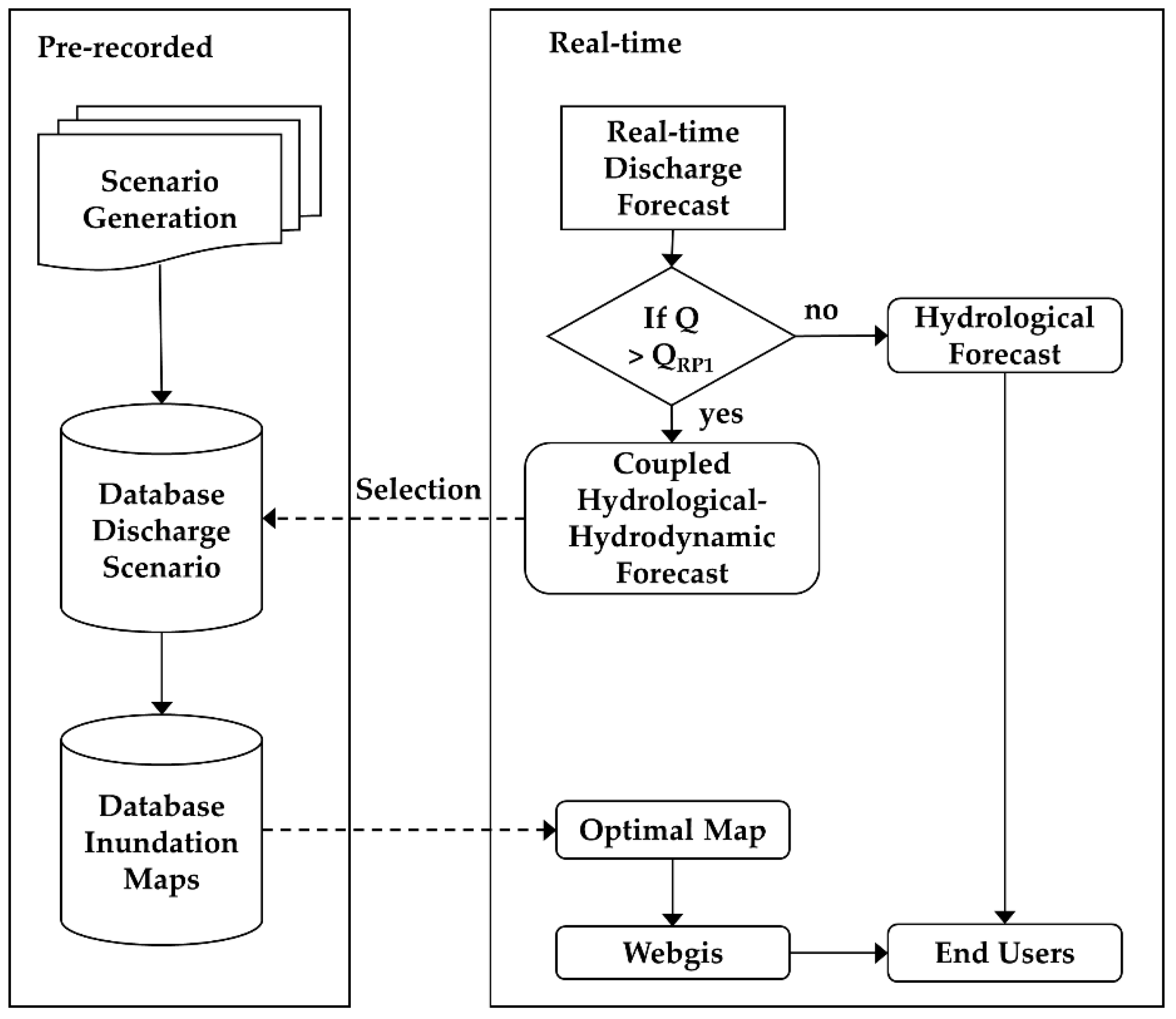
The forecast framework consists of two components: Pre-recorded, where the database was generated and stored; and real-time, in which the optimal inundation map is selected based on real-time discharge forecast (Figure 1).
The pre-recorded component contains databases of the discharge hydrographs and the inundation maps. Synthetic rainfall scenarios were used as an input to generate the discharge database. The scenarios were generated using rainfall intensities, duration, and distributions. Discharge scenarios were generated in two steps: first, the genesis of the discharge hydrograph was modelled using the hydrological model LARSIM (Large Area Runoff Simulation Model) [19]. The model is operationally used in the flood forecasting centre for the river Main at the Bavarian Environment Agency [20]. In the next step, various synthetic convective and advective discharge hydrographs (explained in Section 3.2) were selected from the existing hydrographs based on the peak discharge ranging between the one-year return period and the extreme event, which is 1.5–1.6 times the 100-year return period. The selected hydrographs were further used as the input boundary conditions for the 2D hydrodynamic model HEC-RAS 2D, version 5.0.3 (Hydrologic Engineering Center-River Analysis System, Davis, CA, USA). Altogether, 180 convective and advective scenarios were realised and stored in the discharge database. The maps for the scenarios were stored in the inundation maps database. The generated maps contain high-resolution spatial and temporal (15 min) information of water depth and velocity in the study area. To automatize the component, a tool “FloodEvac” was developed in MATLAB R2018a (version 9.4.0.813654, 64 bit, MathWorks Inc., Natick, MA, USA) [21].
In real-time, the discharge is forecasted for the upstream gauges by the Water Management Authority, Hof, and can be obtained from the LARSIM (Large Area Runoff Simulation Model) model [4]. If the peak of the forecasted discharge is lower than the threshold of a one-year return period (QRP1), only the discharge forecast is shown to the end users. Coupled hydrological-hydrodynamic forecast is activated if the forecasted discharge exceeds the threshold. The threshold of QRP1, which is less than the bankful discharge, is carefully selected to ensure that all the maps begin with the similar initial inundation extent and are not over-spilling the river banks. To select the optimal map from the database, the forecasted hydrograph for the next 12 h is compared to the discharge database and the index of the best match is recorded. Furthermore, the inundation maps corresponding to the recorded index are published for the next 12 h with 15-min intervals and can be accessed by end users via a webgis server. The maps are updated every three hours and the forecasted discharge is matched with the discharge database repeatedly for the next 12 h.
2.2. Evaluation Metrics
To identify similarities between the real-time discharge forecast and the pre-recorded discharge database, two goodness of fit were identified: Nash-Sutcliffe efficiency (NSE) and weighted coefficient of determination (wr2) [22]. The metrics are calculated as in Table 1.
The query to find the best match follows a sequential if-then order. It first selects the best NSE value of more than 0.85 from the database. If no match is found, it selects the best wr2 values of more than 0.85. The value of 0.85 was based on the review for model evaluation criteria between the simulated and measured discharge [22,23]; however, the value can be changed depending on the case study. Furthermore, if no optimal match is found, it selects the best NSE and a warning note is issued to the end-user along with the NSE value reported.
The hindcasted inundation maps for four historical events were generated from the 2D hydrodynamic model. These maps are termed online forecasts in this study. The historical discharges at the upstream gauges were used as the input boundary conditions for the 2D hydrodynamic model. Due to the absence of the real observed flood extents [24], the online inundation maps were used to validate the framework. The results between the selected optimal offline inundation maps were compared to the online maps. To assess the differences in the forecasted inundation extents in the offline and the online maps, Fit Statistic (F) [25] and absolute error (e) was used for flooded cells. A cell is defined as flooded if the water depth in it is more than 0.10 m.
Moreover, the absolute error does not provide information if the offline selected map is over- or under-predicting the inundation. Therefore, errors between the offline and online water depths are also included in the assessment. Positive values indicate an over-prediction and negative values indicate an under-prediction of the water depths. The goodness of fit was calculated over time for the intervals of 15 min as the hydrodynamic model output interval was 15 min.
3. Study Area, Data and Models
3.1. Study Area
The proposed methodology was applied in the city of Kulmbach located in the North-East of the Free State of Bavaria in Southern Germany. The city is crossed by the river White Main and a diversion canal for flood protection, the Mühl canal. Schorgast is one of the main tributaries that meets the White Main upstream of the city. In the north, the small tributary Dobrach meets the White Main and from the south side, two stormwater canals meet the Mühl canal. The river Red Main merges with the White Main near Kulmbach from the South to form the river Main, the longest tributary of the Rhine. Main gauging stations upstream of the city are Ködnitz at White Main and Kauerndorf located at the river Schorgast. For the study, a virtual gauge (Figure 2) was added just after the confluence of the rivers for discharges comparison purposes (Section 4).
The land use is shown in Figure 2a and it generally consists of agricultural land (62%) that includes floodplains and grassland. The water bodies make up 7% of the total model area and include river channel and lakes. The urban area covers around 26% and includes industrial and residential areas as well as transport infrastructures like roads and railway tracks, whereas forests form barely 5% of the total area. The quality of inundation maps depends crucially on the topography. Topography data for this study was provided by the Water Management Authority, Hof (Figure 2b).
3.2. Case Study Data
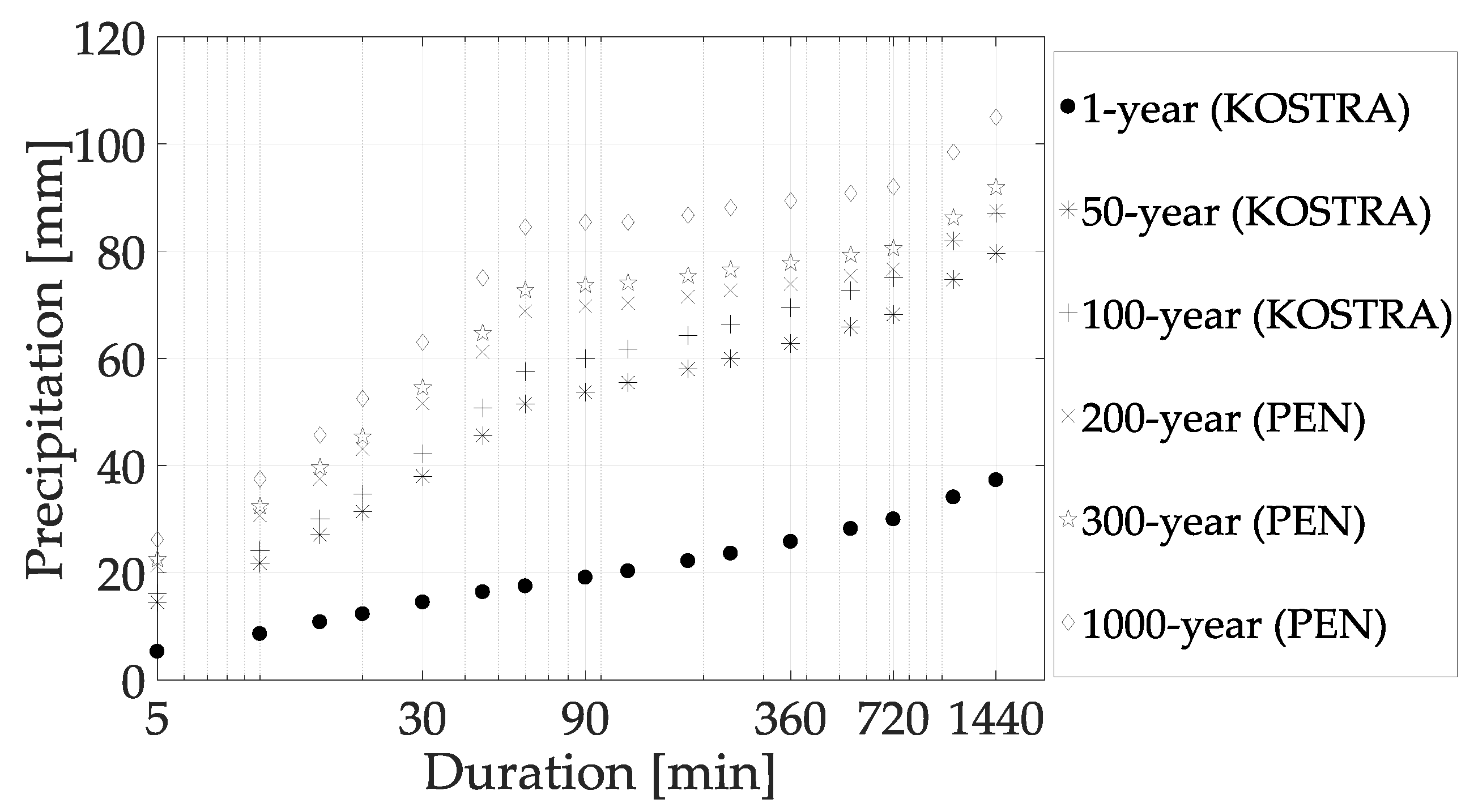
Rainfall probability data was available from the computer program KOSTRA-DWD 2000 (KOordinierte STarkniederschlags-Regionalisierungs-Auswertungen; itwh GmbH Hannover, Germany), which is distributed by the German Meteorological Services (DWD). It provides rainfall intensities for different annual probabilities and durations. It was primarily developed for the design of water management systems such as urban drainage infrastructure or flood retention basins. Precipitation heights were extrapolated using PEN-LAWA 2000 (Praxisrelevante Extremwerte des Niederschlags; itwh GmbH, Hannover, Germany) [26] for the higher return periods. Figure 3 shows the duration and intensities of the precipitation for the city of Kulmbach.
Hydrological measurement data for the historical events were gathered by the Bavarian Hydrological Services and via field surveys. Figure 4a,b shows four historical discharges at two gauges upstream of the city, Ködnitz and Kauerndorf, respectively. The figures also indicate the flood frequency estimations of 1, 5, 20, 50 and 100-year return period discharges along with the extreme event. The historical discharges were used as the input boundary conditions to the online 2D hydrodynamic model, which is later used to show the performance of the offline maps. The events have seasonal characteristics based on convective and advective precipitation input. The hydrographs resulting from a convective precipitation are categorised by higher peaks and shorter duration (May 2006 and May 2013), where the precipitation event can take 25–120 m and rain intensity can vary between 5–60 mm/h [27]. May 2006 and May 2013 had higher peaks and shorter durations and were of convective nature. In May 2013, only the gauge Ködnitz was flooded. The two events that occurred in winter (February 2005 and January 2011) had low peaks but longer durations and were categorised as advective events. An advective precipitation event can last up to 3–4 days and the intensity is often less than 2–3 mm/h [27]. The two categories give a clear indication of convective storm generated from a cloud-burst and snowmelt-rainfall induced flood event. The four events were used to validate the proposed offline forecast.
3.3. Pre-Calibration and Validation of the 2D Flood Inundation Model
HEC-RAS 2D was used as the 2D hydrodynamic model to produce the inundation maps. The model uses an implicit finite difference solution algorithm to discretise time derivatives and hybrid approximations, combining finite differences and finite volumes to discretise spatial derivatives [28]. We used the diffusive wave equations to generate the database due to the less complex numerical schemes and faster calculations [29]. The governing equations are as follows:
where H is the surface elevation (m), h is the water depth (m), u and v are the velocity components in the x- and y-direction, respectively (m/s), q is a source/sink term, g is the gravitational acceleration (m/s2), cf is the bottom friction coefficient (/s), R is the hydraulic radius (m), |V| is the magnitude of the velocity vector (m/s) and n is the Manning’s roughness coefficient (s/m(1/3)).
The model was set up using data provided by the Water Management Authority in Hof and field surveys. The water enters the model domain from the east at rivers White Main (Ködnitz) and Schorgast (Kauerndorf) and flows through the city and meets river Red Main (Unterzetlitz) after the city. The hydrograph boundary conditions represent the observed discharges that enter the simulation domain. Along with the major rivers, four canals were also represented as discharge hydrograph type. Besides the flow hydrograph, an energy slope value of 0.0096 mm−1 was used for distributing the discharge over the cells that integrate the boundary. Table 2 shows the model properties and information of the cell size. The roughness parameter was selected based on a sensitivity analysis. Table 3 shows the calibrated parameter for each land use class (Figure 2a).
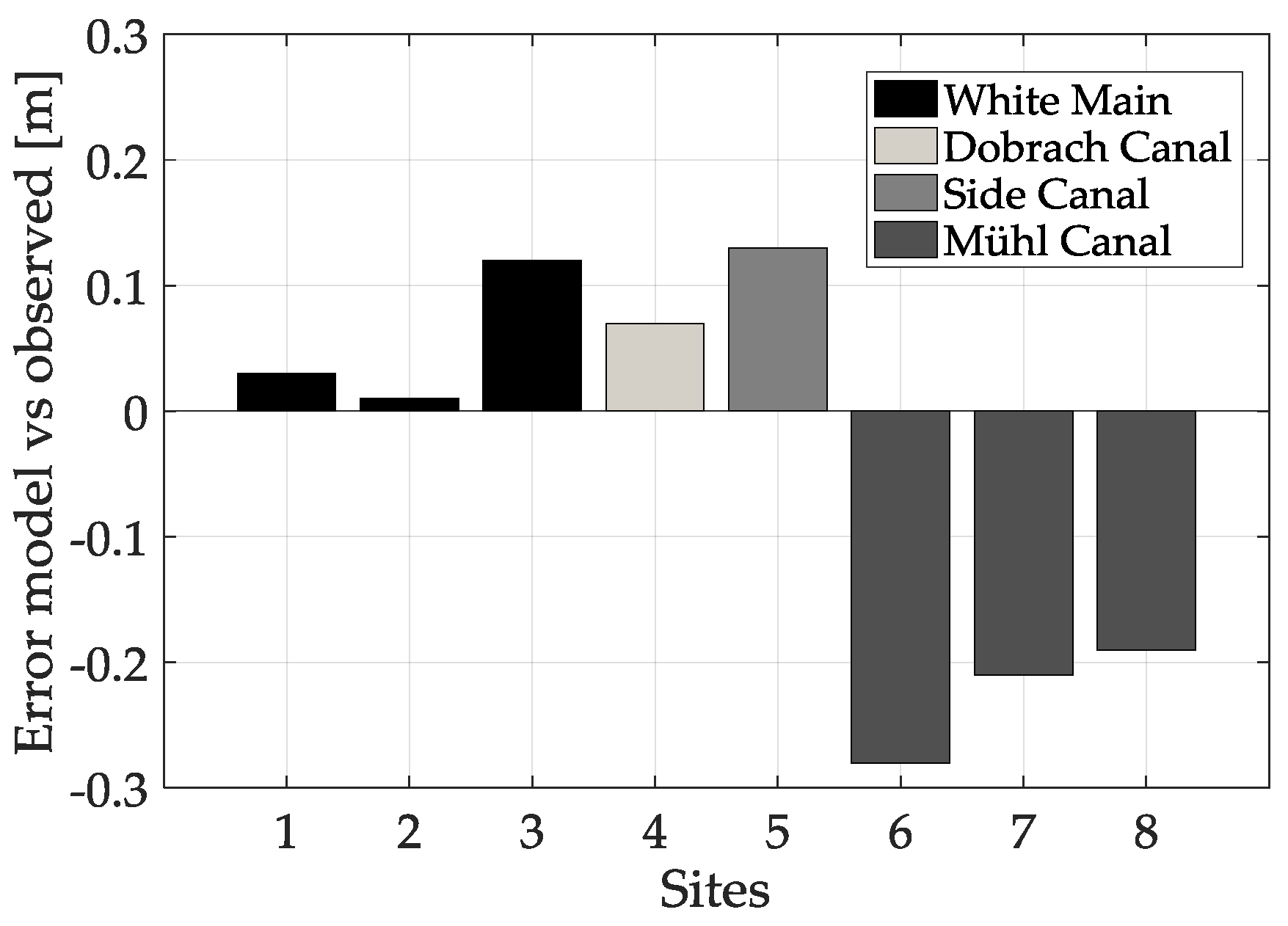
The authority also carried out data collections during the winter flood on 14 January 2011. Water levels were measured at eight bridges in the city of Kulmbach. Since the measured water levels were available for the winter event in January 2011, it was used to calibrate the hydrodynamic model to produce the inundation maps. Figure 5 presents the error between the calibrated HEC-RAS 2D water levels and measured water levels for the eight sites in the city. The model results are in good agreement with the measured data. The sites lying directly on the river White Main (sites 1, 2 and 3) have a good match with a maximum over-prediction of 0.12 m at site 3. Underestimation of up to 0.28 m was observed in the Mühl canal at site 6 and an over-prediction of 0.13 m in the side canal at site 4.
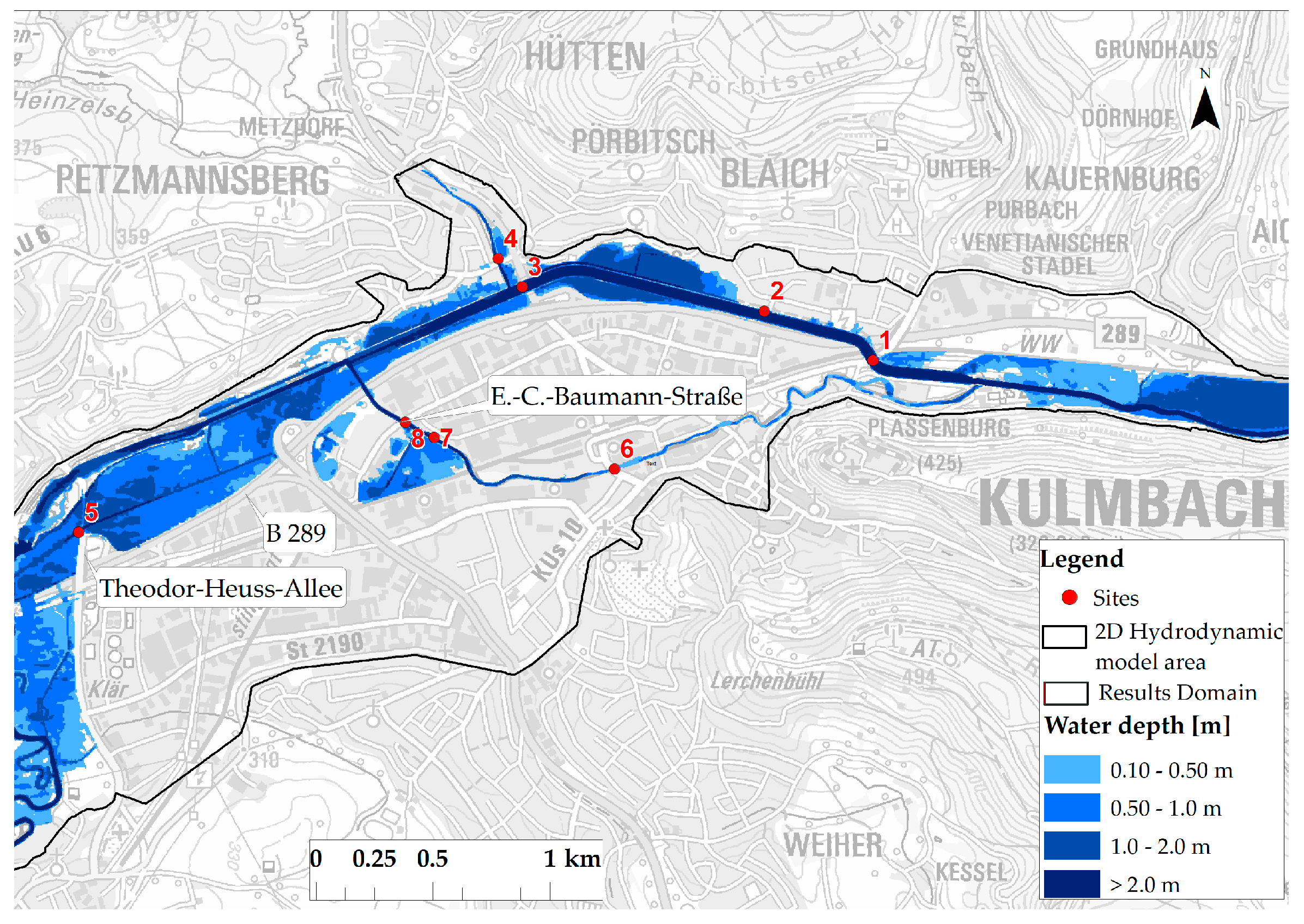
The validation was conducted using binary information of the flood extent that is collected from newspaper articles and press releases from the water authority. Figure 6 shows the resulted inundation map of the city Kulmbach, focused on the eight sites. In the January 2011 event, agricultural land and traffic routes were flooded, but no serious damage was reported. The street Theodor-Heuss-Allee at site 5 was flooded, as well as motorway B 289; the dykes were at their full capacity [30]. Inundation was also reported at sites 7 and 8 around the street E.-C.-Baumann-Straße [31], as supported by the modelling results. Most of the inundation areas are within the floodplains and inundation extent matches with on-field measured data. In general, considering the simple model structure of the HEC-RAS 2D, which disregards the sewer network and urban key features [32], the results were considered satisfactory.
4. Results and Discussion
4.1. Discharge Comparison
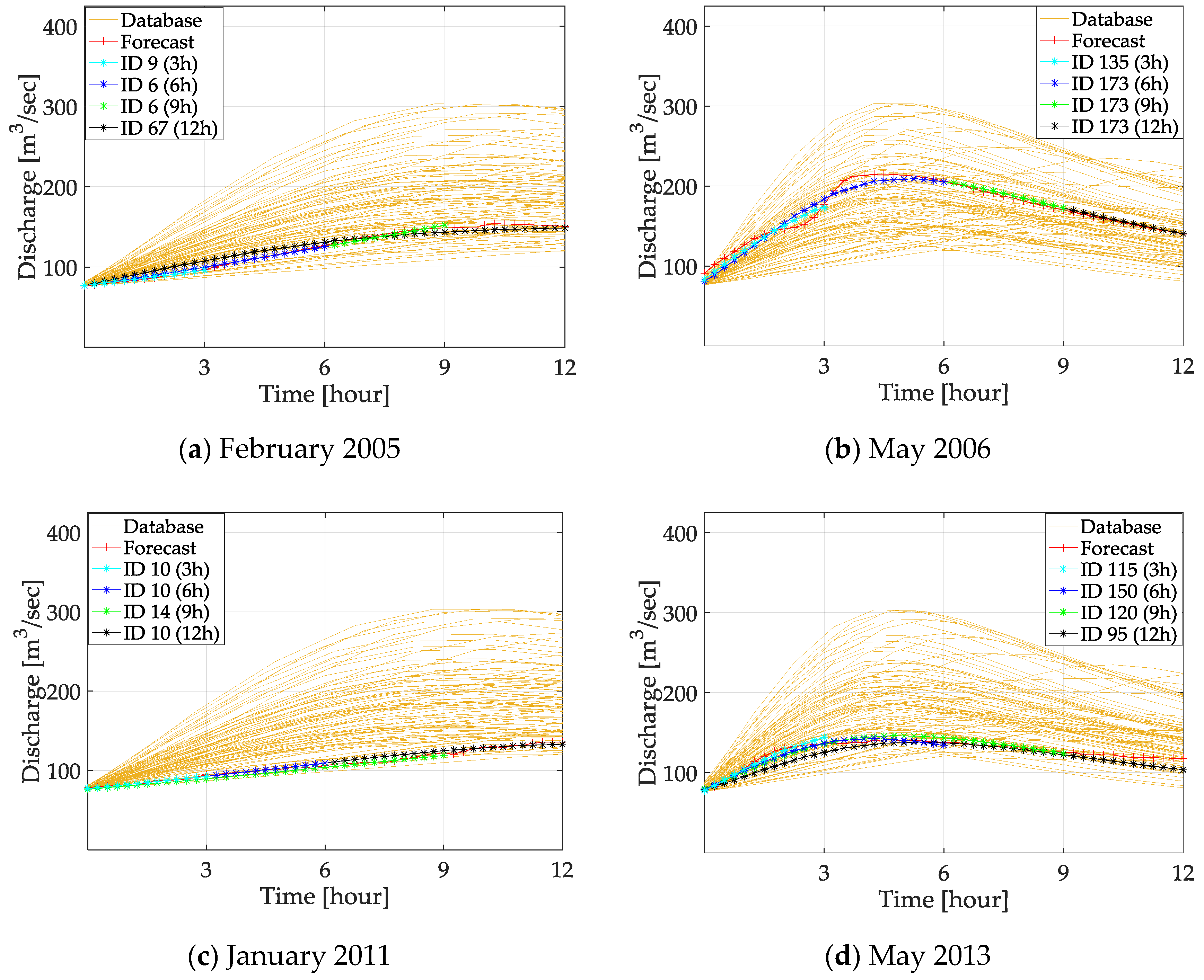
The proposed methodology was validated on four historical hydrological events. Since the discharge forecast in real-time is given for 12 h in advance on the upstream gauges, the inundation forecast duration was set the same and the selection of the maps was updated at every three-hour interval. To incorporate the contribution of both the rivers—Schorgast and White Main—a virtual gauge (Figure 2) was added just after the confluence of the rivers for discharge comparison. The goodness of fits between the forecasted discharge and discharge database at the virtual gauge for the events at every three-hour interval are summarized in Table 4. The discharge dataset was available at every 15 minutes’ interval, which gives 12 data samples to calculate the goodness of fit for each three-hour forecast. The optimal map for each event was found by the query (Section 2.2). Only once was the NSE reported lower than 0.85 and the maps with wr2 of 0.87 were selected at the twelfth hour in May 2013. Figure 7 presents the discharge hydrographs that are resulted from the rainfall scenario at the virtual gauge and the optimal ID for the 12-h forecast window with the three-hour update interval of the four events. The selection of new maps (ID) can be seen in the figure. It also shows the different databases for the advective and convective events. It is worth mentioning that the excellent agreement between the offline and online discharge hydrographs is a result of the suitability of the variety of synthetic scenarios generated from the KOSTRA and PEN rainfall simulation to fit the observed data. The quality of the database is therefore considered equally important as the methodology for selecting the maps, as presented in order to cover possible future events.
4.2. Inundation Forecast Comparison
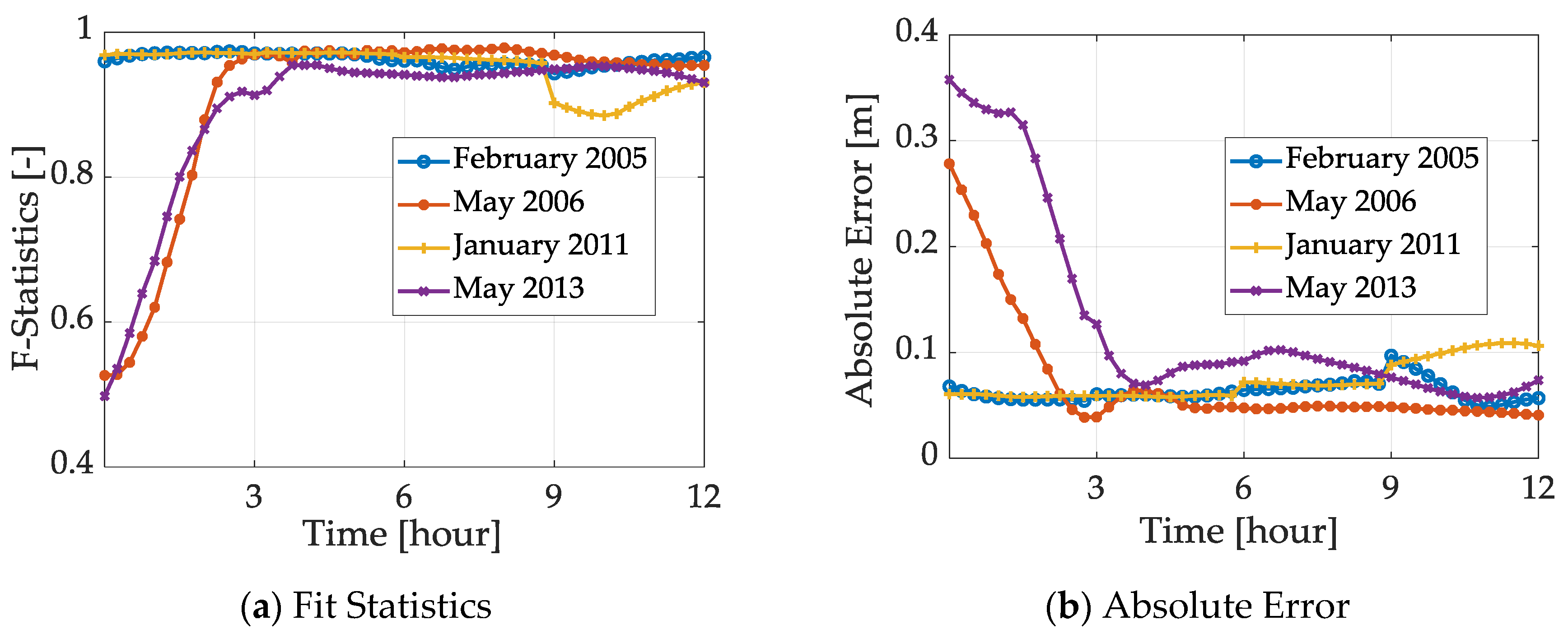
The offline and online inundation maps were compared in the result domain shown in Figure 2. The offline inundation maps produced using the discharge comparison are valid only for the area downstream of the virtual gauge. The inundation maps in the regions between the existing gauges and virtual gauge is produced by comparing the discharge at their respective gauge. Table 5 shows the Fit Statistics and absolute error averaged for the update interval of three hours. In the paper, we assume a deviation up to 0.25 m between offline and online water depth as a threshold, although this value can be changed depending on the requirements of the end-user. Figure 8 shows the metrics with time intervals of 15 min. The spatial extent of the error between offline and online forecast maps are also plotted to see the over- and under-prediction of water depths. Information on the number of flooded cells and the distribution of error in the cells is given in Table 6 and Table 7. The results will be further discussed in the following subsections.
4.2.1. Convective Events
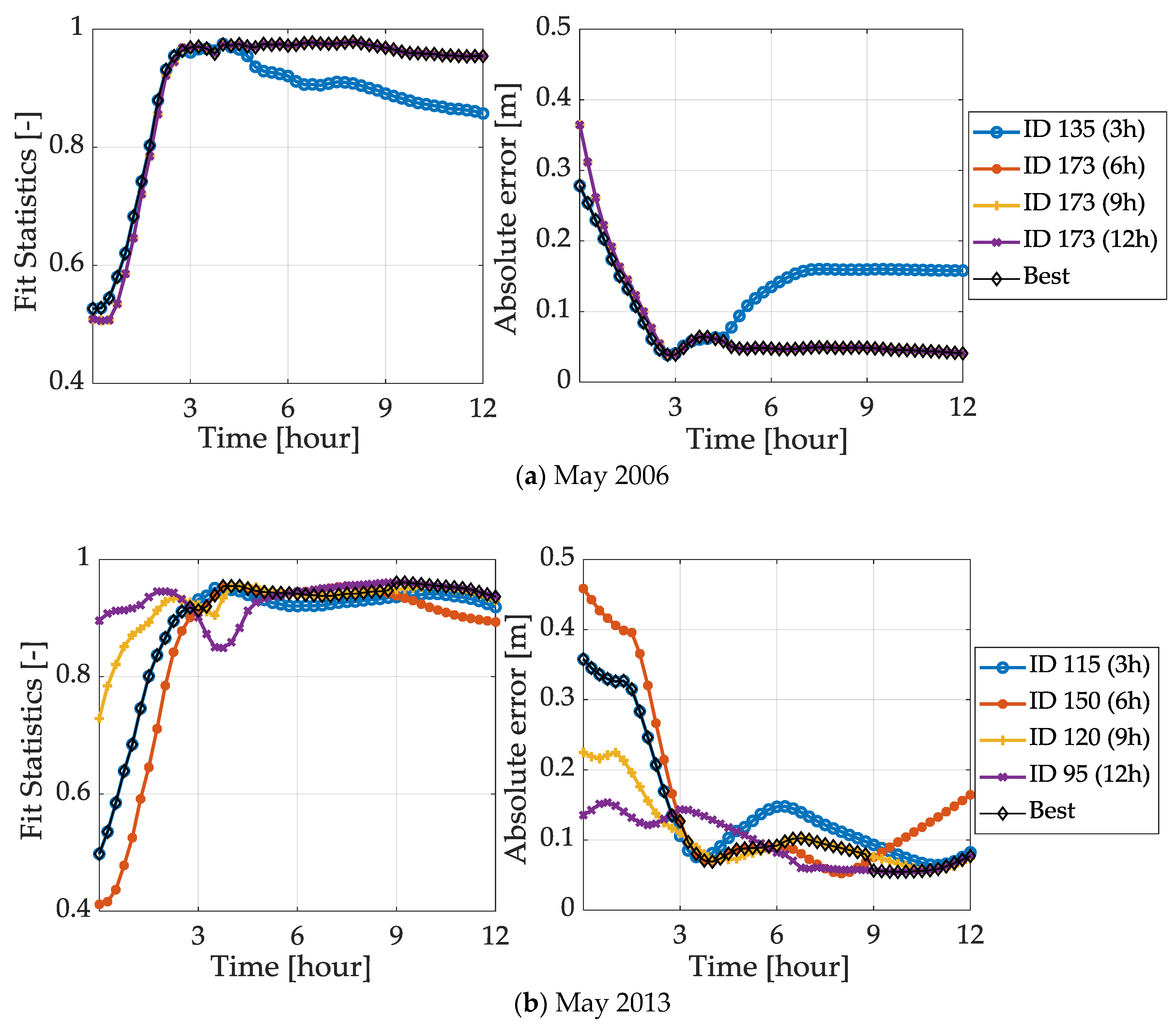
The events in May 2006 and May 2013 were categorised as convective events and the results for both events show similar trends. They start with a poor average F (0.75 and 0.76) and average e (0.14 and 0.27 m), but as the time increases, the performance gets better. Figure 7b,d show that the discharge compared well with NSE value of 0.91 and 0.97 at the third hour in May 2006 and 2013 respectively. However, the inundation maps show discrepancies between offline and online maps. This was induced from the one-year return period threshold at the beginning of the forecast. As we look further—the spatial extent of the error between offline and online maps—the results show a satisfactory agreement.
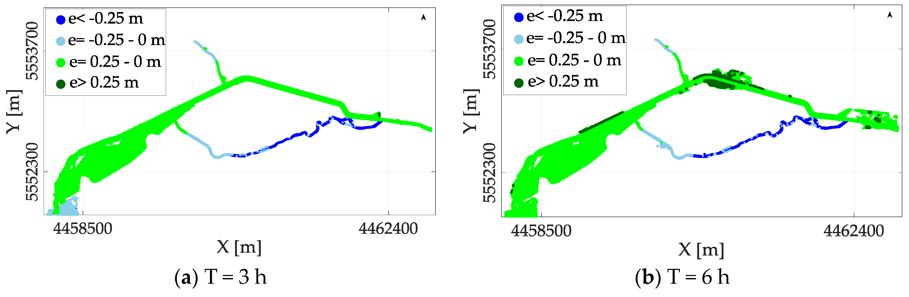
May 2006 was an extreme hydrological event and both the upstream gauges reached a discharge corresponding to the 100-year return period (Figure 4). The protection structures were breached, and critical infrastructure was flooded. Almost 31% of the cells in the result domain were flooded at the twelfth hour (Table 6), which is the highest amount in all four events. The spatial extent of error in Figure 9 and Table 6 show that the difference was mostly within the acceptable limit of 0.25 m at all times. Only 3% of cells lying in the Mühl canal were found under-predicting the water depths by more than 0.25 m. The water depths were under-predicted at initial hours but as the peak of the flood passed and the number of flooded cells increased (after the sixth hour), the water depths were over-predicted. It can be concluded that the extreme event was predicted quite well using the offline forecast.
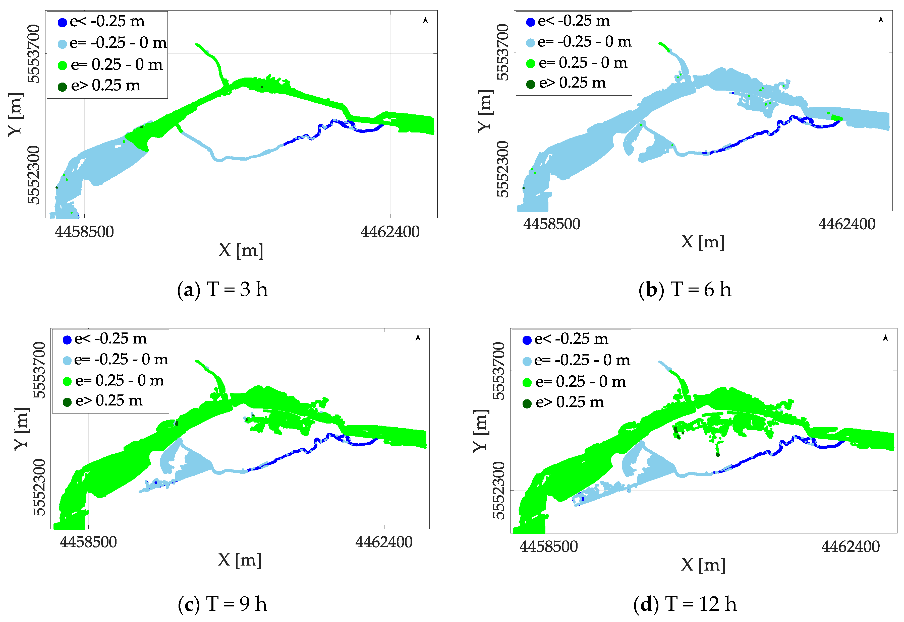
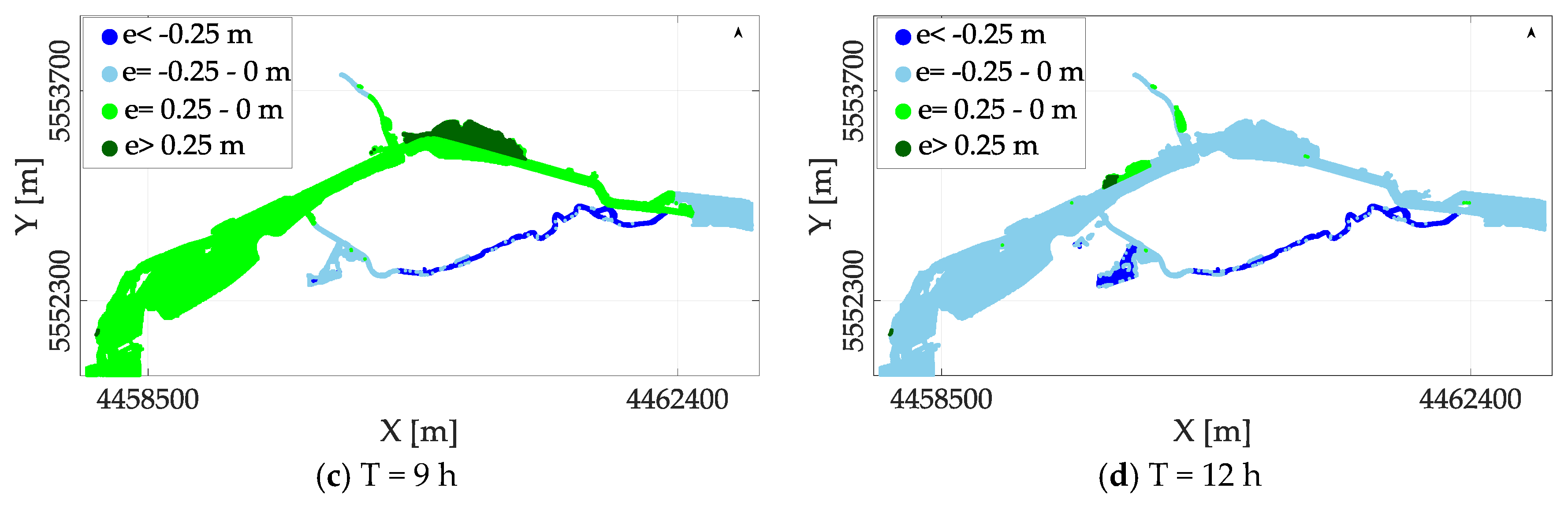
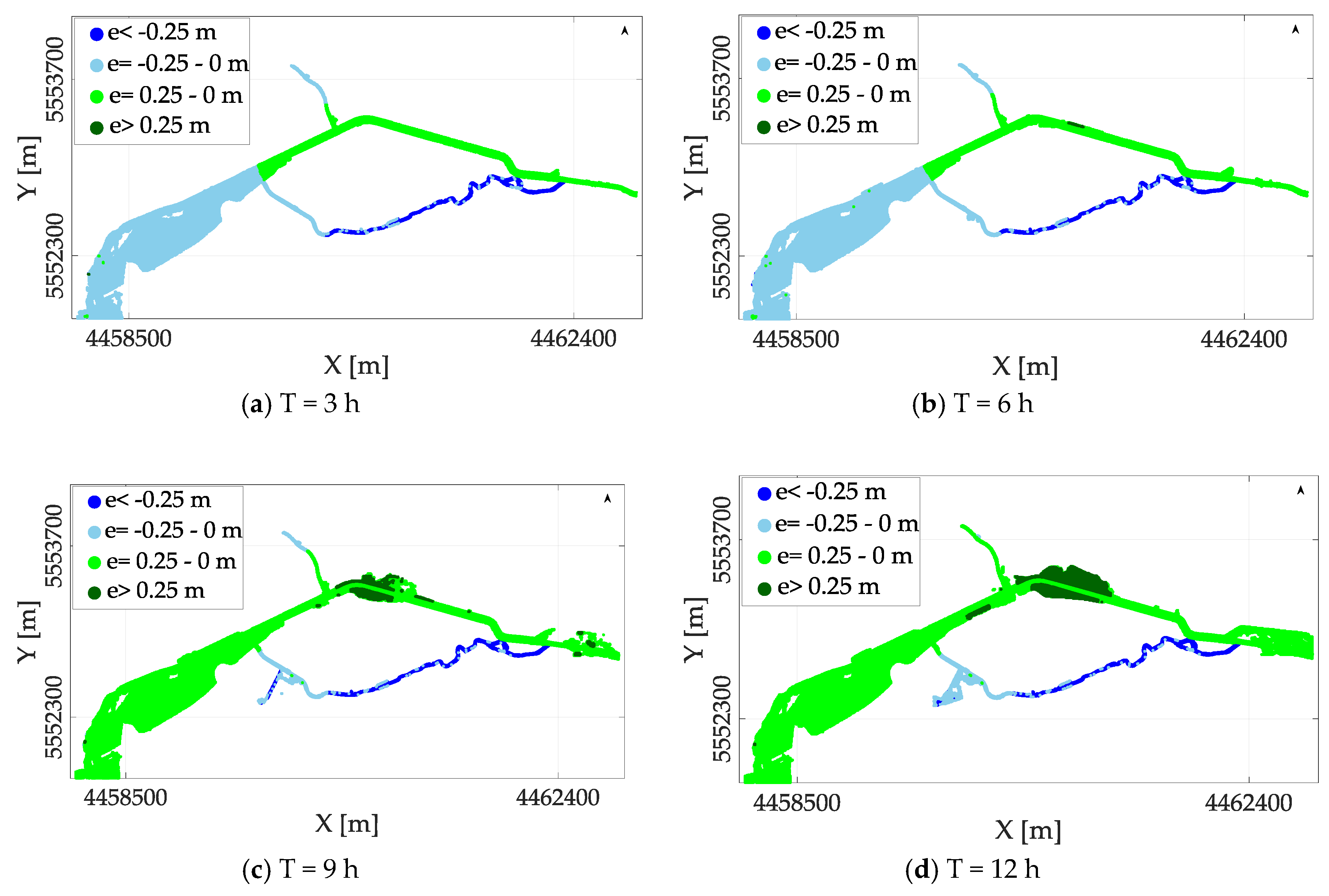
In May 2013, however, only one of the upstream gauges at Ködnitz was flooded (Figure 4b), therefore discharge was considerably low at the virtual gauge. The number of flooded cells is also lower than in May 2006. F and e show average performance at initial stages with average F values of 0.76, 0.80 and average e values of 0.27 and 0.22 m at the third and sixth hour. As the time increases, the performance gets better. The spatial extent of error (Figure 10) and Table 7 suggest under-prediction at the third hour, with 8% of the cells with an error of more than 0.25 m. At the sixth hour, 7% of the cells over-predicted the water depths on the river Upper Main and 5% of the cells that lie on the Mühl canal did the same. At the ninth and twelfth hour, performance improved in the river and only 4% and 8% of cells, respectively, under-predicted the water levels at the Mühl canal. Additional under-predicted cells are clustered at the junction of the Mühl canal and E.-C.-Baumann-Straße and over-predicted cells in the floodplains on the river Upper Main.
4.2.2. Advective Events
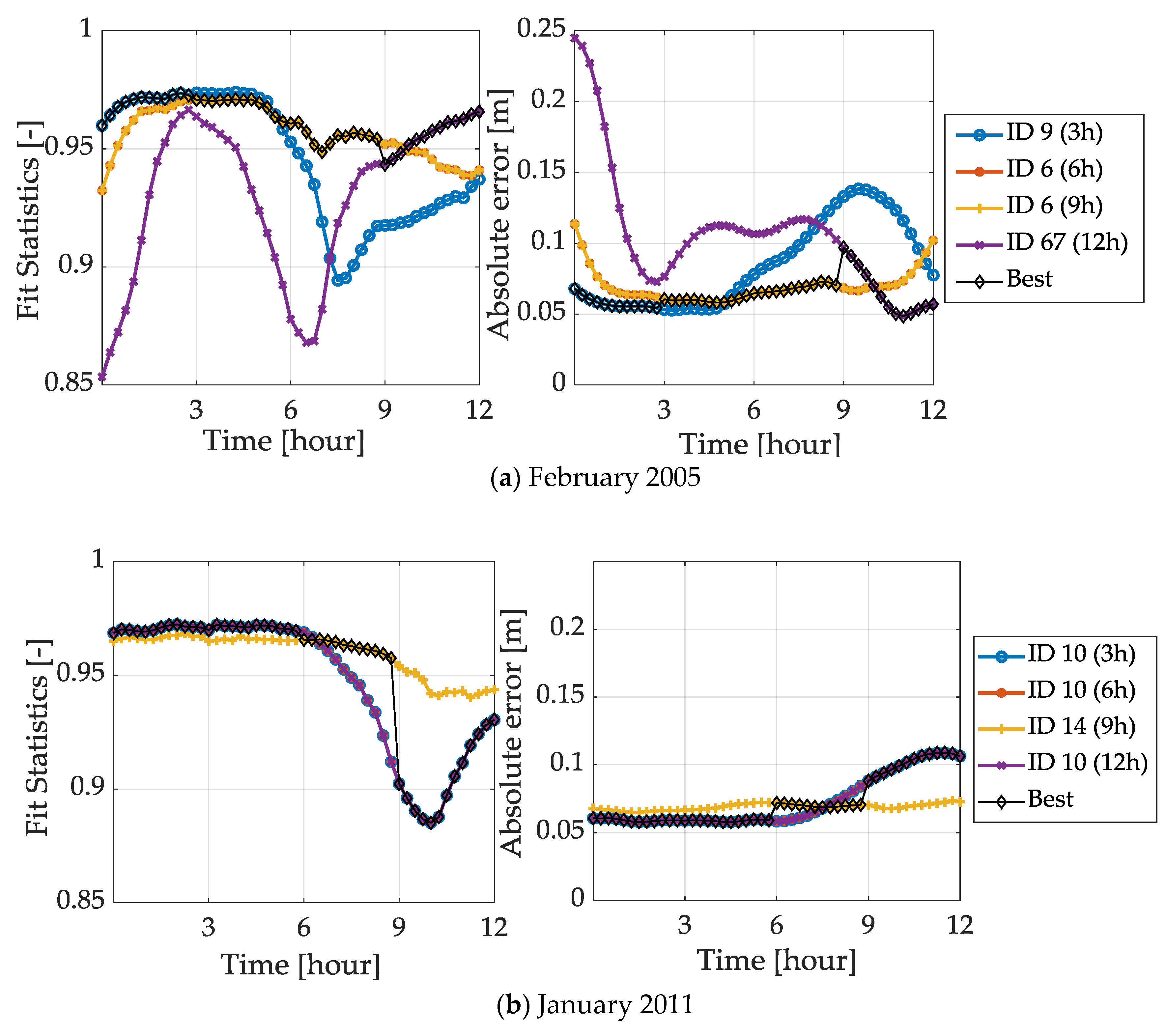
The advective events exhibit similar characteristics such as long duration and flatter peak (Figure 4). Unlike the convective events, both goodness of fits F and e are good from the beginning and stay much within the acceptable limits, with a minimum value of average F of 0.93 and 0.95, and minimum average e of 0.11 and 0.07 m at the twelfth hour for the two events in 2005 and 2011, respectively. In Figure 8, both F and e after the ninth hour indicate a decrease in the performance for January 2011. F returns to an acceptable value at the twelfth hour; however, the error remains the same. Similar trends can be seen in February 2005, in which e deviates after the ninth hour but returns to 0.05 m. Spatial distribution of error (Figure 11 and Figure 12) suggests slight under-prediction in all time steps in the Mühl canal and slight over-prediction at the river Upper Main. Table 8 and Table 9 show the percentage error distribution of the advective events. In February 2005, only 7% of the cells were over-predicted more than 0.25 m at the ninth hour (similar pattern for May 2013). In January 2011, the agreement was good until the ninth hour, when the over-prediction of water depth started (10% at the twelfth hour). However, it was restricted to the floodplain of the river at the northern part. Overall, a good agreement was reached between offline and online inundation maps.
4.3. Update Map Selection
Updating the selection of maps is an important step to avoid selecting offline inundation maps that do not provide optimal results. With an update, a new set of maps was selected every three hours for the next twelve hours. The changes in the performance of the four validation events are plotted in Figure 13 and Figure 14 for convective and advective events, respectively. The figures show F and e values of the events at every time step along with the index (ID) of the database. It also shows the best match or the maps selected for the forecast duration. For the convective events, as described in the previous section, the start was not perfect, but the performance improves with time.
In the convective event of May 2006, only two indexes—ID 135 for 0–3 h and ID 173 for 6–12 h—were selected. The change in the third hour was important in order to find the optimal maps available with the highest F and least e. In May 2013, for the initial 0–3 h, better performance maps (ID 95) were available, but it selected ID 115 because of the high threshold for which the forecast starts (76 m3/s). This value was decided on the river overflowing the banks. Since the inundation extents are within the main channel, they are not affected by this initial discharge. It would be possible to reduce this value and optimise the forecasts. The optimal maps were selected from 3–12 h.
The update was also successful in advective events. In February 2005 (Figure 14a), at all the time steps, it selected the best performance maps with the highest F and least e. In January 2011, optimal maps were selected for 0–9 h, however, for 9–12 h, the optimal maps were not selected (Figure 14b). This happens because the map selection is based on the optimal discharge hydrographs selection. This may not be the case for the corresponding inundation maps. The online inundation maps may be closer to another discharge scenario in the database. The difference between the maps was however not drastic and both maps were well within the threshold of 0.25 m (Section 4.2).
5. Framework Performance
The framework has shown to be robust and efficient for operational flood forecast, both in terms of time and cost-effectiveness, when compared to an online inundation forecast. Indeed, this methodology overcomes the main constraints of online forecast, namely the need for the use of supercomputers and maintenance of infrastructure [8], as well as the limitation on the computational time required by 2D hydrodynamic models. In addition, the resolution (cell size) or scale of the maps are not a limiting factor in this offline methodology; in principle, the resolution is limited by available data. Had we used online modus, the 2D hydrodynamic model would have required 30 min to simulate a real-time event of 12 h on an 8-core, 2.4 GHz (Intel E5-2665), including the initial start. Post-processing of the model results and update of the maps on the webgis server would consume an additional 15 min. Therefore, online inundation maps would only be delivered to decision makers 45 min after the discharge forecast at the upstream gauges for the next 12 h. The proposed offline framework, by contrast, runs in seconds to find the best selection of the maps and as such, it can be used as an early warning system. The maps are forwarded to a webgis server, where they are published, and end-users can see them in fine resolution.
A disadvantage of the framework is the error in water volume introduced by the update of the map selection. The water volume changes every time a different discharge is selected. This issue does not occur for online forecasts. The jump in the map outputs (water depth and velocities) occurs after every three-hour update and will be more or less pronounced, depending on the difference between the previous and the new discharge scenarios. We acknowledge that this is an additional source of uncertainty when compared to online forecasts. However, only 0–10% of the flooded cells exceeded 0.25 m. This difference can nonetheless be minimised by increasing the number of scenarios. In addition, regular updates of the inundation database are required in case of major land use, construction changes in the city, and climate change. In any case, the current database can be easily improved by including the simulation of historical events as well as performing a continuous update of new events.
6. Conclusions
A framework for an offline flood forecast has been presented, which overcomes the high computational time required by hydrodynamic flood forecasting. The framework was validated using four extreme historical hydrological events. A total of 180 convective and advective scenarios were simulated, as compared to the 44 scenarios used in the ESPADA system [16]. The forecast duration was 12 h and a new set of inundation maps was selected every three hours using real-time discharge forecasts as input. Furthermore, the map selection in real-time can improve the given forecast and substantially reduce errors. We thus conclude that the methodology works for both convective and advective events with a threshold of 0.25 m water depth. The current database has limitations and it needs to be enlarged to incorporate multiple peak events. Future work will see the generation of additional discharge scenarios based on historical data to strengthen the proposed framework.
A major advantage of the forecasting framework is its fast run-time and its easy application to other study areas, regardless of their size. This methodology can be applied to virtually any catchment size. The 2D hydrodynamic model run-times are not a limitation since all runs are prepared beforehand. In the study, the inundation maps were compared downstream at a virtual gauge that is introduced to incorporate the contribution of both the rivers. In a complex river system, an ensemble of inundation maps can be provided by comparing the discharge at existing gauges and at virtual gauges, introduced at the confluence of rivers. The ease of operational practise of the offline systems is well documented in previous applications such as ESPADA system in France, the Zambezi FloodDSS in Mozambique, in which the inundation database was produced using a 1D hydraulic model [15], and EFAS in Sara river basin [17]. Furthermore, there are major challenges in operational application of these systems, in particular: Recompilation of the database in major land-use changes, an exhaustive database to cover all possible scenarios, validation of the query to select the most optimal scenario, and real-time validation of the forecast.
At an urban scale, the availability of real-time inundation maps would substantially improve emergency responses by assessing potential consequences of forecasted events [33], and the end users of early warning systems would indeed benefit from prioritising and coordinating evacuation planning. Typical end-users are disaster relief organisations, such as the Federal Agency for Technical Relief (THW), the German Red Cross, and the Bavarian Water Authorities. For advanced users such as decision-makers in water management authorities, the published inundation maps should furthermore serve as a tool for better risk assessment.
In addition, even though we applied a simpler model (diffusive wave), it can easily be adapted to full dynamic models, since there is no limitation on the computational time. Future work will see the inclusion of a 1D-2D sewer/overland flow coupled-model and extend the method to forecasting urban pluvial flooding [24], including radar rainfall as an additional input in the query [8].
A further promising application that is being tested is to incorporate both offline and online in one framework. In cases where a satisfactory goodness of fit is not found (<0.85) between the real-time discharge forecast and the discharge database, the online modus is activated, the 2D hydrodynamic model is run in real-time, and maps are made available. This will lead to fewer resource consumption as compared to a complete online forecast and reduced errors in the outputs. Furthermore, pre-calculated dynamic inundation maps can help to visualise the uncertainties in the hydrodynamic modelling and support rescue services. Better flood mitigation and flood forecast planning strategies can be developed by visualising inundation scenarios for different magnitudes of floods and associated potential damage for various quantiles of discharge hydrographs.
Author Contributions
For research articles with several authors, a short paragraph specifying their individual contributions must be provided. The following statements should be used “Conceptualization, P.K.B., J.L. and M.D.; Methodology P.K.B.; Software, P.K.B.; Validation, P.K.B.; Formal Analysis, P.K.B.; Investigation, P.K.B.; Resources, P.K.B. and M.D.; Data Curation, P.K.B.; Writing-Original Draft Preparation, P.K.B.; Writing-Review & Editing, P.K.B., J.L. and M.D.; Visualization, P.K.B.; Supervision, J.L. and M.D. Project Administration, P.B, J.L.; Funding Acquisition, M.D.”, please turn to the CRediT taxonomy for the term explanation. Authorship must be limited to those who have contributed substantially to the work reported.
Funding
This research was funded by the German Federal Ministry of Education and Research (BMBF) with the grant number FKZ 13N13196.
Acknowledgments
The authors would like to thank all contributing project partners, funding agencies, politicians, and stakeholders in different functions in Germany. A very special thanks to the Bavarian Water Authority and Bavarian Environment Agency in Hof for providing us with quality data to conduct the research. We would also like to thank the language centre of the Technical University of Munich for their consulting in English writing.
Conflicts of Interest
The author declares no conflict of interest.
References
- European Commission. Directive 2007/60/EC of the European Parliament and of the Council of 23 October 2007 on the Assessment and Management of Flood Risks. 2007. Available online: https://eur-lex.europa.eu/legal-content/EN/TXT/PDF/?uri=CELEX:32007L0060&from=EN (accessed on 23 March 2018).
- Munich Re. Topics GEO Natural Catastrophes 2016—Analyses, Assessments, Positions; Münchener Rückversicherung-Gesellschaft (Munich Re): Munich, Germany, 2017. [Google Scholar]
- Thieken, A.H.; Kienzler, S.; Kreibich, H.; Kuhlicke, C.; Kunz, M.; Mühr, B.; Müller, M.; Otto, A.; Petrow, T.; Pisi, S.; et al. Review of the Flood Risk Management System in Germany after the Major Flood in 2013. Ecol. Soc. 2016, 21, 1–12. [Google Scholar] [CrossRef]
- Laurent, S.; Hangen-Brodersen, C.; Ehret, U.; Meyer, I.; Moritz, K.; Vogelbacher, A.; Holle, F.K. Forecast Uncertainties in the Operational Flood Forecasting of the Bavarian Danube Catchment. In Hydrological Processes of the Danube River Basin—Perspectives from the Danubian Countries; Brilly, M., Ed.; Springer: Dordrecht, The Netherlands, 2010; pp. 367–387. [Google Scholar]
- Bates, P.D.; Pappenberger, F.; Romanowicz, R.J. Uncertainty in Flood Inundation Modelling. In Applied Uncertainty Analysis for Flood Risk Management; Beven, K., Hall, J., Eds.; Imperial College Press: London, UK, 2014; pp. 232–269. [Google Scholar]
- Hu, X.; Song, L. Hydrodynamic Modeling of Flash Flood in Mountain Watersheds Based on High-performance GPU Computing. Nat. Haz. 2018, 91, 567–586. [Google Scholar] [CrossRef]
- Zhang, S.; Yuan, R.; Wu, Y.; Yi, Y. Parallel Computation of a Dam-break Flow Model Using Openacc Applications. J. Hydraul. Eng. 2017, 143, 04016070. [Google Scholar] [CrossRef]
- Henonin, J.; Russo, B.; Mark, O.; Gourbesville, P. Real-time Urban Flood Forecasting and Modelling—A State of the Art. J. Hydroinform. 2013, 15, 717–736. [Google Scholar] [CrossRef]
- Bhatt, C.M.; Rao, G.S.; Diwakar, P.G.; Dadhwal, V.K. Development of Flood Inundation Extent Libraries Over a Range of Potential Flood Levels: A Practical Framework for Quick Flood Response. Geomat. Nat. Haz. Risk 2017, 8, 384–401. [Google Scholar] [CrossRef]
- Voigt, S.; Kemper, T.; Riedlinger, T.; Kiefl, R.; Scholte, K.; Mehl, H. Satellite Image Analysis for Disaster and Crisis-management Support. IEEE Trans. Geosci. Remote Sens. 2007, 45, 1520–1528. [Google Scholar] [CrossRef]
- Bates, P.D. Integrating Remote Sensing Data with Flood Inundation Models: How Far Have We Got? Hydrol. Process 2012, 26, 2515–2521. [Google Scholar] [CrossRef]
- Bales, J.D.; Wagner, C.R. Sources of Uncertainty in Flood Inundation Maps. J. Flood Risk Manag. 2009, 2, 139–147. [Google Scholar] [CrossRef]
- René, J.-R.; Djordjević, S.; Butler, D.; Madsen, H.; Mark, O. Assessing the Potential for Real-time Urban Flood Forecasting Based on a Worldwide Survey on Data Availability. Urban Water J. 2014, 11, 573–583. [Google Scholar] [CrossRef]
- Chen, A.S.; Hsu, M.-H.; Teng, W.-H.; Huang, C.-J.; Yeh, S.-H.; Lien, W.-Y. Establishing the Database of Inundation Potential in Taiwan. Nat. Haz. 2006, 37, 107–132. [Google Scholar] [CrossRef] [Green Version]
- Schulz, A.; Kiesel, J.; Kling, H.; Preishuber, M.; Petersen, G. An Online System for Rapid and Simultaneous Flood Mapping Scenario Simulations—The Zambezi FloodDSS. Presented at the EGU General Assembly Conference, Vienna, Austria, 12–17 April 2015. [Google Scholar]
- Raymond, M.; Peyron, N.; Bahl, M.; Martin, A.; Alfonsi, F. ESPADA: Un Outil Innovant Pour la Gestion en Temps Réel Descrues Rrbaines. In Proceedings of the Novatech 6th Conference of Sustainable Techniques and Strategies in Urban Water Management, Lyon, France, 25–27 June 2007; pp. 793–800. [Google Scholar]
- Dottori, F.; Kalas, M.; Salamon, P.; Bianchi, A.; Alfieri, L.; Feyen, L. An Operational Procedure for Rapid Flood Risk Assessment in Europe. Nat. Haz. Earth Syst. Sci. 2017, 17, 1111–1126. [Google Scholar] [CrossRef]
- Alfieri, L.; Salamon, P.; Bianchi, A.; Neal, J.; Bates, P.; Feyen, L. Advances in Pan-European Flood Hazard Mapping. Hydrol. Proc. 2014, 28, 4067–4077. [Google Scholar] [CrossRef]
- Ludwig, K.; Bremicker, M. The Water Balance Model LARSIM: Design, Content and Applications; Institut für Hydrologie der Universität: Freiberg, Germany, 2006. [Google Scholar]
- Disse, M.; Konnerth, I.; Bhola, P.K.; Leandro, J. Unsicherheitsabschätzung für die Berechnung von Dynamischen Überschwemmungskarten—Fallstudie Kulmbach. Wasserwirtsch. Springer Prof. 2017, 11, 47–51. [Google Scholar] [CrossRef]
- Leandro, J.; Konnerth, I.; Bhola, P.; Amin, K.; Köck, F.; Disse, M. Floodevac Interface zur Hochwassersimulation mit Integrierten Unsicherheitsabschätzungen. In Tag der Hydrologie, Fachgemeinschaft Hydrologische; Reinhardt-Imjela, C., Ed.; Wissenschaften in der DWA Geschäftsstelle: Trier, Germany, 2017; pp. 185–192. [Google Scholar]
- Krause, P.B.; Boyle, D.P.; Bäse, F. Comparison of Different Efficiency Criteria for Hydrological Model Assessment. Adv. Geosci. 2005, 5, 89–97. [Google Scholar] [CrossRef]
- Moriasi, D.; Arnold, J.; Van Liew, M.; Bingner, R.; Harmel, R.D.; Veith, T. Model Evaluation Guidelines for Systematic Quantification of Accuracy in Watershed Simulations. Trans. ASABE 2007, 50, 885–900. [Google Scholar] [CrossRef]
- Leandro, J.; Djordjević, S.; Chen, A.S.; Savić, D.A.; Stanić, M. Calibration of a 1D/1D Urban Flood Model Using 1D/2D Model Results in the Absence of Field Data. J. Water Sci. Technol. 2011, 64, 1016–1024. [Google Scholar] [CrossRef]
- Moya Quiroga, V.; Kure, S.; Udo, K.; Mano, A. Application of 2D Numerical Simulation for the Analysis of the February 2014 Bolivian Amazonia Flood: Application of the New HEC-RAS Version 5. RIBAGUA Rev. Iberoam. Agua 2016, 3, 25–33. [Google Scholar] [CrossRef]
- Verworn, H.R. Praxisrelevante Extremwerte des Niederschlags; Institut für Wasserwirtschaft, Hydrologie und Landwirtschaftlichen Wasserbau: Magdenburg, Germany, 2016; pp. 173–185. [Google Scholar]
- Maniak, U. Niederschlag-abfluss-modelle für Hochwasserabläufe. In Hydrologie und Wasserwirtschaft: Eine Einführung für Ingenieure; Springer: Berlin, Germany, 2010; pp. 261–360. [Google Scholar]
- Brunner, G.W. HEC-RAS River Analysis System Hydraulic Reference Manual; Report for US Army Corps of Engineers; Hydrologic Engineering Center (HEC): Davis, CA, USA, 2010. [Google Scholar]
- Leandro, J.; Chen, A.S.; Schumann, A. A 2D Parallel Diffusive Wave Model for Floodplain Inundation with Variable Time Step (P-D Wave). J. Hydrol. 2014, 517, 250–259. [Google Scholar] [CrossRef]
- Hof, W. Flood Events of January 2011 in Main. Available online: www.wwa-ho.bayern.de/hochwasser/hochwasserereignisse/januar2011/main/index.htm (accessed on 20 March 2018).
- Wolf, L. Hochwassergroßeinsatz in Kulmbach. Available online: https://fotothurnau.wordpress.com/2011/01/15/hochwasser-groseinsatz-in-kulmbach/ (accessed on 20 March 2018).
- Leandro, J.; Schumann, A.; Pfister, A. A Step Towards Considering the Spatial Heterogeneity of Urban Key Features in Urban Hydrology Flood Modelling. J. Hydrol. 2016, 535, 356–365. [Google Scholar] [CrossRef]
- Molinari, D.; Ballio, F.; Handmer, J.; Menoni, S. On the Modeling of Significance for Flood Damage Assessment. Int. J. Disaster Risk Reduct. 2014, 10, 381–391. [Google Scholar] [CrossRef]
Figure 1.
Framework of the offline flood inundation forecast including the pre-recorded and real time component. The coupled hydrological-hydrological forecast is activated once a one-year return period (QRP1) is exceeded.
Figure 1.
Framework of the offline flood inundation forecast including the pre-recorded and real time component. The coupled hydrological-hydrological forecast is activated once a one-year return period (QRP1) is exceeded.

Figure 2.
Study area (a) Land use and (b) digital elevation model of the city Kulmbach. Data source: Water Management Authority Hof.
Figure 2.
Study area (a) Land use and (b) digital elevation model of the city Kulmbach. Data source: Water Management Authority Hof.

Figure 3.
Precipitation values in mm for various durations (in min) and various return periods. PEN method used to extrapolate precipitation values above 100-year return period. Data source: KOSTRA-DWD 2000 (Kulmbach: Column 47, Row 67).
Figure 3.
Precipitation values in mm for various durations (in min) and various return periods. PEN method used to extrapolate precipitation values above 100-year return period. Data source: KOSTRA-DWD 2000 (Kulmbach: Column 47, Row 67).

Figure 4.
Discharge hydrographs at the upstream gauging stations (a) Ködnitz and (b) Kauerndorf. Data source: Bavarian Hydrological Service (www.gkd.bayern.de).
Figure 4.
Discharge hydrographs at the upstream gauging stations (a) Ködnitz and (b) Kauerndorf. Data source: Bavarian Hydrological Service (www.gkd.bayern.de).

Figure 5.
Error in m between the water levels resulting from the calibrated model and the measured water levels on 14 January 2011 at eight sites.
Figure 5.
Error in m between the water levels resulting from the calibrated model and the measured water levels on 14 January 2011 at eight sites.

Figure 6.
Inundation map of the city of Kulmbach on 14 January 2011 at 14:00.

Figure 7.
Comparison of discharge hydrographs at the virtual gauge: (a,c) advective events in February 2005 and January 2011, (b,d) convective events in May 2006 and May 2013.
Figure 7.
Comparison of discharge hydrographs at the virtual gauge: (a,c) advective events in February 2005 and January 2011, (b,d) convective events in May 2006 and May 2013.

Figure 8.
Goodness of fit (a) Fit Statistics and (b) Absolute Error between offline and online flooded cells for each time step for the forecast duration of 12 h.
Figure 8.
Goodness of fit (a) Fit Statistics and (b) Absolute Error between offline and online flooded cells for each time step for the forecast duration of 12 h.

Figure 9.
Water depth error between offline and online maps for May 2006. Positive values indicate over-prediction and negative values indicate under-prediction: (a) T = 3 h, (b) T = 6 h, (c) T = 9 h and (d) T = 12 h.
Figure 9.
Water depth error between offline and online maps for May 2006. Positive values indicate over-prediction and negative values indicate under-prediction: (a) T = 3 h, (b) T = 6 h, (c) T = 9 h and (d) T = 12 h.

Figure 10.
Water depth error between offline and online maps for May 2013: (a) T = 3 h, (b) T = 6 h, (c) T = 9 h and (d) T = 12 h.
Figure 10.
Water depth error between offline and online maps for May 2013: (a) T = 3 h, (b) T = 6 h, (c) T = 9 h and (d) T = 12 h.

Figure 11.
Water depth error between offline and online for February 2005: (a) T = 3 h, (b) T = 6 h, (c) T = 9 h and (d) T = 12 h.
Figure 11.
Water depth error between offline and online for February 2005: (a) T = 3 h, (b) T = 6 h, (c) T = 9 h and (d) T = 12 h.


Figure 12.
Water depth error between offline and online for January 2011: (a) T = 3 h, (b) T = 6 h, (c) T = 9 h and (d) T = 12 h.
Figure 12.
Water depth error between offline and online for January 2011: (a) T = 3 h, (b) T = 6 h, (c) T = 9 h and (d) T = 12 h.

Figure 13.
Update of the map selection for the convective events: (a) May 2006 and (b) May 2013.

Figure 14.
Update of the map selection for the advective events: (a) February 2005 and (b) January 2011.
Figure 14.
Update of the map selection for the advective events: (a) February 2005 and (b) January 2011.


Table 1.
Evaluation metrics used in the study.
| Evaluation Metrics | Equation | Terms |
|---|---|---|
| Nash-Sutcliffe efficiency (NSE) | —the number of samples —the forecasted discharge —the discharge of the database —the gradient of the regression line | |
| Weighted coefficient of determination (wr2) | ||
| Fit Statistic (F) | —the overlap of flooded cells in the online () and offline () maps —the number of flooded cells and —the water depth in the offline and online maps | |
| Absolute Error (e) |
Table 2.
2D hydrodynamic model properties.
| Data | Value |
|---|---|
| Model area | 11.5 km2 |
| Total number of cells | 430,485 |
| Number of cells in results domain | 193,161 |
| Δt | 20 s |
| Minimum cell area | 6.8 m2 |
| Maximum cell area | 59.8 m2 |
| Average cell area | 24.8 m2 |
Table 3.
Manning’s M for each land use class.
| Land Use | Calibrated Manning’s n [s/m(1/3)] | Ranges of Manning’s n [s/m(1/3)] |
|---|---|---|
| Water bodies | 0.022 | 0.015–0.149 |
| Agriculture | 0.043 | 0.025–0.110 |
| Forest | 0.189 | 0.110–0.200 |
| Transportation | 0.014 | 0.012–0.020 |
| Urban | 0.074 | 0.040–0.080 |
Table 4.
Goodness of fit for discharge comparison.
| Duration | No. of Data Samples | Goodness of Fit [-] | |||
|---|---|---|---|---|---|
| February 2005 | May 2006 | January 2011 | May 2013 | ||
| 0–3 h | 13 | 0.98 (NSE) | 0.91 (NSE) | 0.96 (NSE) | 0.97 (NSE) |
| 0–6 h | 25 | 0.99 (NSE) | 0.95 (NSE) | 0.97 (NSE) | 0.96 (NSE) |
| 0–9 h | 37 | 0.99 (NSE) | 0.95 (NSE) | 0.95 (NSE) | 0.91 (NSE) |
| 0–12 h | 49 | 0.94 (NSE) | 0.95 (NSE) | 0.97 (NSE) | 0.87 (wr2) |
Table 5.
Average Fit Statistics and absolute error for the four events at the end of the forecast update interval of three hours.
Table 5.
Average Fit Statistics and absolute error for the four events at the end of the forecast update interval of three hours.
| Duration | Average Fit Statistics [-] | Average Absolute Error [m] | ||||||
|---|---|---|---|---|---|---|---|---|
| February 2005 | May 2006 | January 2011 | May 2013 | February 2005 | May 2006 | January 2011 | May 2013 | |
| 0–3 h | 0.97 | 0.75 | 0.97 | 0.76 | 0.06 | 0.14 | 0.06 | 0.27 |
| 0–6 h | 0.96 | 0.84 | 0.97 | 0.80 | 0.07 | 0.11 | 0.06 | 0.22 |
| 0–9 h | 0.96 | 0.89 | 0.97 | 0.92 | 0.07 | 0.09 | 0.07 | 0.12 |
| 0–12 h | 0.93 | 0.90 | 0.95 | 0.93 | 0.11 | 0.08 | 0.07 | 0.11 |
Table 6.
Percentage of cells inundated at the convective event in May 2006.
| Time | Flooded Cells | May 2006 [%] | |||
|---|---|---|---|---|---|
| <−0.25 m | −0.25–0 m | 0.25–0 m | >0.25 m | ||
| T = 3 h | 36,865 | 3 | 48 | 49 | 0 |
| T = 6 h | 55,550 | 3 | 96 | 1 | 0 |
| T = 9 h | 60,012 | 3 | 11 | 86 | 0 |
| T = 12 h | 60,418 | 3 | 13 | 84 | 0 |
Table 7.
Percentage of cells inundated at the convective event in May 2013.
| Time | Flooded Cells | May 2013 [%] | |||
|---|---|---|---|---|---|
| <−0.25 m | −0.25–0 m | 0.25–0 m | >0.25 m | ||
| T = 3 h | 34,493 | 8 | 92 | 0 | 0 |
| T = 6 h | 44,553 | 5 | 4 | 84 | 7 |
| T = 9 h | 45,864 | 4 | 6 | 89 | 1 |
| T = 12 h | 44,204 | 8 | 88 | 3 | 1 |
Table 8.
Percentage of inundated cells at the advective event in February 2005.
| Time | Flooded Cells | February 2005 [%] | |||
|---|---|---|---|---|---|
| <−0.25 m | −0.25–0 m | 0.25–0 m | >0.25 m | ||
| T = 3 h | 30,915 | 6 | 7 | 87 | 0 |
| T = 6 h | 37,426 | 5 | 2 | 87 | 5 |
| T = 9 h | 43,691 | 5 | 12 | 76 | 7 |
| T = 12 h | 46,790 | 7 | 91 | 2 | 0 |
Table 9.
Percentage of inundated cells at the advective event in January 2011.
| Time | Flooded Cells | January 2011 [%] | |||
|---|---|---|---|---|---|
| <−0.25 m | −0.25–0 m | 0.25–0 m | >0.25 m | ||
| T = 3 h | 30,825 | 6 | 70 | 24 | 0 |
| T = 6 h | 32,348 | 6 | 69 | 25 | 0 |
| T = 9 h | 37,097 | 6 | 3 | 87 | 4 |
| T = 12 h | 42,603 | 5 | 4 | 81 | 10 |
© 2018 by the authors. Licensee MDPI, Basel, Switzerland. This article is an open access article distributed under the terms and conditions of the Creative Commons Attribution (CC BY) license (http://creativecommons.org/licenses/by/4.0/).
Share and Cite
MDPI and ACS Style
Bhola, P.K.; Leandro, J.; Disse, M. Framework for Offline Flood Inundation Forecasts for Two-Dimensional Hydrodynamic Models. Geosciences 2018, 8, 346. https://doi.org/10.3390/geosciences8090346
AMA Style
Bhola PK, Leandro J, Disse M. Framework for Offline Flood Inundation Forecasts for Two-Dimensional Hydrodynamic Models. Geosciences. 2018; 8(9):346. https://doi.org/10.3390/geosciences8090346
Chicago/Turabian StyleBhola, Punit Kumar, Jorge Leandro, and Markus Disse. 2018. "Framework for Offline Flood Inundation Forecasts for Two-Dimensional Hydrodynamic Models" Geosciences 8, no. 9: 346. https://doi.org/10.3390/geosciences8090346
Note that from the first issue of 2016, this journal uses article numbers instead of page numbers. See further details here.