HF/VHF Radar Sounding of Ice from Manned and Unmanned Airborne Platforms

Abstract

Ice thickness and bed topography of fast-flowing outlet glaciers are large sources of uncertainty for the current ice sheet models used to predict future contributions to sea-level rise. Due to a lack of coverage and difficulty in sounding and imaging with ice-penetrating radars, these regions remain poorly constrained in models. Increases in off-nadir scattering due to the highly crevassed surfaces, volumetric scattering (due to debris and/or pockets of liquid water), and signal attenuation (due to warmer ice near the bottom) are all impediments in detecting bed-echoes. A set of high-frequency (HF)/very high-frequency (VHF) radars operating at 14 MHz and 30–35 MHz were developed at the University of Kansas to sound temperate ice and outlet glaciers. We have deployed these radars on a small unmanned aircraft system (UAS) and a DHC-6 Twin Otter. For both installations, the system utilized a dipole antenna oriented in the cross-track direction, providing some performance advantages over other temperate ice sounders operating at lower frequencies. In this paper, we describe the platform-sensor systems, field operations, data-processing techniques, and preliminary results. We also compare our results with data from other ice-sounding radars that operate at frequencies both above (Center for Remote Sensing of Ice Sheets (CReSIS) Multichannel Coherent Depth Sounder (MCoRDS)) and below (Jet Propulsion Laboratory (JPL) Warm Ice Sounding Explorer (WISE)) our HF/VHF system. During field campaigns, both unmanned and manned platforms flew closely spaced parallel and repeat flight lines. We examine these data sets to determine image coherency between flight lines and discuss the feasibility of forming 2D synthetic apertures by using such a mission approach.

1. Introduction

Glaciers in both Greenland and Antarctica are undergoing significant changes due to a changing climate. While it is well-established that mass losses from these polar ice sheets contribute to global sea-level rise (SLR) [1], there remains great uncertainty about how these contributions will change in the future. In their 5th Assessment Report, the Intergovernmental Panel on Climate Change (IPCC) reports that mean global sea level could increase anywhere from 28 (RCP2.6) to 98 cm (RCP8.5) by the end of the century, and glaciers are expected to contribute anywhere from 15–55% of this projected range [2]. Recent satellite measurements and paleoclimate records suggest future SLR could be even greater than the IPCC predictions [3,4,5]. Since roughly 150 million people live within 1 m of the current sea level [6], our ability to accurately predict future SLR is crucial to effectively plan, adapt, and mitigate the socio-economic consequences of our changing climate.

Ice sheet models are our primary tool for integrating observations in predictions of polar ice contributions to future SLR. These models predict future trends in mass balance through ice thickness, snow accumulation, and ice velocities derived from satellite measurements. Jacobs et al. [7] and Larour et al. [8] suggest that ice thickness and bed elevation are the most important model parameters in reducing model uncertainties; even small uncertainties in ice thickness can lead to large biases in discharge estimates.

For several decades, specially designed radars have proven to be effective tools not only for sounding and imaging the ice bedrock [9,10,11,12,13], but also for mapping internal layers and measuring snow accumulation on land and sea ice [14,15]. Sounder data has also been used to extract other glaciological information such as the basal thermal state [16,17,18], internal layering that provides insight into ice dynamics [19], and characterizing basal roughness [20]. Several large-scale airborne radar campaigns have been organized in an attempt to address the need for ice bedrock and thickness measurements in both Greenland and Antarctica over the last decade, including the National Aeronautics and Space Administration (NASA) Program for Arctic Regional Climate Assessment (PARCA) [21] and NASA Operation Ice Bridge (OIB) [22,23,24]. OIB utilizes a suite of radars—developed by the Center for Remote Sensing of Ice Sheets (CReSIS) at the University of Kansas—operating from 150 MHz to 38 GHz to provide a full profile of the ice column [25]. One of these radars is CReSIS’s Multichannel Coherent Depth Sounder (MCoRDS), a wideband very high-frequency (VHF) radar operating from 160–230 MHz for sounding ice and imaging the ice-bedrock interface.

In addition to CReSIS’s MCoRDS system, several other groups have developed airborne VHF sounders that have also contributed to mapping the ice thickness and underlying bedrock of both Greenland and Antarctica. The Alfred Wegner Institute (AWI) and the British Antarctic Survey (BAS) systems operate at 150 MHz, while systems developed by the University of Texas Institute for Geophysics (UTIG) and Technical University of Denmark (DTU) operate at 60 MHz. While spatial coverage remains an issue in crucial regions across the continent, the systems summarized in

Table 1. Summary of notable very high-frequency (VHF) ice sounders.

Organization Instrument	Center Frequency	Bandwidth	References
AWI	150 MHz	Burst	[26]
BAS/PASIN	150 MHz	10 MHz	[27,28,29]
DTU	60 MHz	4 MHz	[30]
CReSIS/MCoRDS			[25]
1993–2008	150 MHz	20 MHz
2009–current	195 MHz	20–30 MHz
UTIG/HiCARS	60 MHz	15 MHz	[31,32]

(as well as others) contributed to the creation of improved high-resolution bed maps for both Greenland (BedMachine v3 [33]) and Antarctica (Bedmap2 [24]).

Critical regions (such as outlet glaciers and ice-sheet margins) represent a relatively small percentage of the total ice-sheet area, but they are extremely difficult to sound and image and thus remain poorly represented and constrained in models [34,35]. Obtaining measurements from these regions is critical to better understanding ice-sheet dynamics. In particular, bed information near the grounding line of marine-terminating glaciers is important to appropriately constrain numerical flow models used to test marine ice sheet instability (MISI). The hypothesis that glacier retreat on reverse bed slopes can lead to irreversible glacier instability [36] is based on assumptions at the grounding line that are difficult to test due to poor data resolution. These regions are incredibly challenging to sound because increased surface and volumetric clutter masks weak bed echoes. Clutter is much more significant in these regions due to the rough and heavily crevassed surfaces and increased volumetric scattering caused by inclusions (e.g., debris and water pockets) within the ice. Bed returns are also significantly attenuated due to the high water content of the temperate ice.

While there has been some success sounding these critical areas with VHF radars, the performance of radars operating above 50 MHz degrades over the temperate ice within fast-flowing glaciers [37,38,39]. Sounding of these areas suggests the need for lower frequency radars that are inherently less sensitive to scattering features and extinction in the wet ice. As given in Equation (1), the power received from a given target is a function of the target geometry (transmission coefficient through the ice-surface interface, 1 − |Γ_s|²; reflection coefficient of the ice-bed interface, |Γ_ib|²; and ice attenuation losses L_i) and radar system (antenna gain, G; operating wavelength, λ; and transmitted power P_t) characteristics.

$$P_r=\frac{P_t{G}^2{\lambda }^2{(1-{\left|{\mathrm{\Gamma }}_s\right|}^2)}^2{\left|{\mathrm{\Gamma }}_{\mathrm{ib}}\right|}^2}{{(4\pi )}^3{R}^4{L}_i}$$

(1)

The losses associated with a return signal include geometric spreading losses (1/(4π)³R⁴) and attenuation of the electromagnetic wave (L_i) due to dielectric losses and scattering losses from inclusions within the ice; these can be modeled as a loss tangent term with an (a/λ)³ relationship where a is the radius of the inclusions [40]. Furthermore, such inclusions can also contribute to clutter in the form of a volume backscatter, thus limiting bed detection due to clutter interference. Meltwater runoff can result in englacial water pockets whose characteristic lengths are on the order of 1 m [39]. Rayleigh scattering theory suggests the backscatter (loss) is inversely proportional to λ⁴ for inclusions whose circumference is much smaller than a wavelength (2πR << λ) [41]. For situations where volume inclusions limit bed detection, lowering the system operating frequency will reduce attenuation losses as well as volume backscatter to not only increase the desired signal but also reduced the clutter signal; thus, improving the signal to interference and noise ratio (SINR).

In addition, several studies have indicated that ice attenuation is dependent on frequency. MacGregor, et al. [42] suggest that the conductivity of ice (and thus attenuation) is proportional to ω^α where ω is the radial frequency and α is the Cole–Cole distribution parameter. Subsequent studies have also used this frequency-dependent correction factor when considering radar attenuation [43]. Indeed, Paden et al. [44] observed an 8 ± 1.2 dB increase in signal loss between 100 and 500 MHz over the North Greenland Ice Core Project (NGRIP).

These factors suggest that low frequency radars are more likely to detect bed returns where VHF (and higher frequency) radars have not reliably operated. HF radars have reduced Doppler bandwidth and range bandwidth, which can make targets more difficult to interpret and limit the processing gain achievable through synthetic aperture radar (SAR) applications. However, in the regions where HF radars are most likely to be relevant for ice bottom detection, the VHF signal is so heavily defocused by the heterogenous media that the interpretability is similar (see Section 3.1).

Watts and Wright were the first to demonstrate a low frequency (<50 MHz) airborne impulse radar for sounding of temperate ice in 1978 [36]. Despite the limited technology of the time (e.g., no precision positional measurements, analog data recording), the 1.5 MHz system provided some bed profiles and detected the bed to depths greater than 300 m [45]. Since this initial demonstration, several others have demonstrated airborne radars operating from 1 to 30 MHz [46,47,48,49,50]. The Warm Ice Sounding Explorer (WISE) developed by the NASA Jet Propulsion Laboratory (JPL) [48,49] demonstrated temperate ice depth measurements exceeding 1200 m in Alaska, as did a similar system utilized by the University of Washington (UW) [50].

While the reduced sensitivity of HF frequencies to volumetric scattering is an advantage, there are several drawbacks to operating at these lower frequencies—primarily increased noise and required antenna size. Galactic noise is a dominating factor at HF (approximately 58,000 K [51]). It is significantly higher than the primary noise source at VHF, namely thermal noise (due to electronics, which are usually taken to be 290 K). The total noise figure is typically 20 dB higher at HF than thermal noise at 180–210 MHz.

Antenna size is the primary technical challenge of integrating radars operating at lower frequencies than VHF. Both WISE and the UW radars operate with a center frequency between 2–2.5 MHz, and both utilize long (>100 m) resistively loaded wire antennas similar to the concept shown in Figure 1 [49,50]. While the lower operational frequencies are advantageous, there are performance trade-offs for decreased frequency. As compared to the VHF systems in Table 1 utilizing cross-track antenna arrays, typically only a single dipole element can be integrated onto the aircraft, resulting in a very broad radiation pattern. Large off-nadir radiation and spatial sidelobes can significantly degrade SINR, especially when flown over glacier valleys or highly crevassed surfaces. In addition, advanced signal processing with the flexible wire antenna is more difficult due to the uncertainty of the antenna’s phase center location during flight.

CReSIS developed a dual-frequency HF/VHF radar (14/30–35 MHz) for sounding fast-flowing temperate ice. We operated this radar from a manned Twin Otter DCH-6 in Greenland and a miniaturized version from a small unmanned aircraft system (UAS) in both Greenland and Antarctica. Unlike previous airborne temperate ice sounders, the antenna elements for both the manned and UAS systems are oriented perpendicular to the direction of travel (cross-track direction). Equation (2) gives the electric field intensity of a half-wave dipole along its axis. In this equation, j is the imaginary number, I_o is the excitation current, k is the wave number, r is the distance from the source, and θ is the look angle.

$$E\simeq j\eta \frac{I_o{e}^{-jkr}}{2\pi r}\left[\frac{cos\left(\frac{\pi }{2}cos\theta \right)}{sin\theta }\right]$$

(2)

While the dipole radiation pattern is not considered directional and does not have the same surface clutter suppression capabilities as the VHF arrays, there are some performance advantages to this orientation. First, for wire antennas oriented in the along-track direction, any rotation of the antenna will result in small reductions in the nadir bed signal (due to the orientation of the pattern nulls). For an antenna rotation of 30° (a reasonable angle for trailing wire antennas [49]), according to Equations (1) and (2), this would result in a ~3.5 dB reduction in received power from nadir. In the case of the cross-track oriented antenna, the pattern nulls at endfire will result in some additional clutter suppression. According to Equation (2), the antenna pattern would provide between 3.5–20 dB addition clutter suppression for clutter angles between 30°–70°. The orientation of the cross-track pattern is further advantageous since we use traditional SAR techniques to form a narrow-beam in the along-track direction. In addition, it has been suggested that improved clutter suppression is possible for HF radars by flying closely spaced flight lines that can be combined to form a synthetic 2D-aperture. A 2D-aperture would allow for similar beamforming capabilities (and thus clutter suppression) as the multi-element VHF sounders.

In this paper, we describe both the manned and unmanned versions of the system and discuss the results from several field campaigns. Measurements taken with the UAS radar in 2013 represent the first successful sounding of ice with a UAS-based radar [52]. We present preliminary field measurements and compare our results to measurements of radar sounders that operate at both higher (CReSIS MCoRDS) and lower (JPL’s WISE) frequencies. Finally we assess the coherency of multi-pass data taken during our UAS field deployment and discuss the feasibility of synthesizing a 2D-aperture to further improve clutter suppression.

2. Materials and Methods

2.1. Radar Overview

A summary of the parameters of the CReSIS VHF/HF radar (referred to as the HF Sounder) is provided in

Table 2. Center for Remote Sensing of Ice Sheets (CReSIS) very high-frequency/high-frequency radar (HF Sounder) parameters.

Parameter	Twin Otter (TO)	Unmanned Aircraft System (UAS)
Center Operating Frequency (low/high)	14.1 MHz/31.5 MHz	14.6 MHz/34.3 MHz
Bandwidth (low/high) 1	1.1 MHz/8 MHz	1 MH/5 MHz
Transmit Power (peak)	1000 Watts	100 Watts
Pulse Repetition Frequency (programmable)	20 kHz	10 kHz
Pulse Duration	0.35–1 μs	0.32–1 μs
Sampling Rate	200 MS/s (12.5 MHz with DDC)	50 MS/S
Data Rate	75 MB/s max	2 MB/S

¹ Operating bandwidth was limited by the 8 dB width of the antenna response (6 dB width for Band 1) for TO experiment. bandwidths whereas bandwidth for UAS is 10 dB bandwidth.

. Both versions of the radar operate over two discrete frequency bands—14 MHz and 30–35 MHz. The frequencies of operation were selected based on the success of previous systems. The lower frequency band operating around 14 MHz (Band 1) was identified based on the favorable results demonstrated by Arcone (2000) with a 12 MHz radar in Alaska where scattering from volumetric debris is high [53]. The 30–35 MHz mode of the HF sounder (Band 2) was selected based on a 30 MHz design (developed by Blinlow et al. [47]) used to sound 800 m thick temperate ice in Patagonia with heavily crevassed surfaces and melt water ponds. The exact center frequency in both cases was selected based on platform integration, antenna tuning, and frequency spectrum allocation.

Figure 2 shows a simplified block diagram for both the Twin Otter (TO) and miniaturized UAS radar systems. As the figure shows, the system is composed of control, digital, radio frequency (RF), power amp-TR switch (PA/TR), and antenna subsystems.

The digital subsystem includes a high-speed arbitrary waveform generator (AWG) and a 14-bit analog-to-digital converter (ADC). To reduce the data rates, the TO version of the radar has built-in digital down-conversion capabilities, while the UAS version can perform on-board decimation. A wired network connection to a dedicated computer running a graphical user interface (GUI) communicates commands in the TO HF sounder. For the UAS version, a 900 MHz wireless link is used to send simple command, status, and quick-look data packets. A NMEA (National Marine Electronics Association) GGA serial stream from the on-board Global Positioning System (GPS) receiver and a 1 pulse-per-second (PPS) timing signal time-tag the radar data.

The RF section includes low-power analog electronics for both transmitter and receiver. The RF transmitter is composed of a reconstruction filter and driver amplifier (10 W-TO part number MADQ07A fromPolyfet RF Devises, Camarillo, CA, USA; 0.15 W-UAS part number HMC580 Analog Devices, Norwood, MA, USA). The receiver contains a low-noise amplifier, variable gain amp, and anti-aliasing bandpass filter. The PA is capable of outputting more than 1000-W of peak power for the TO version and 100-W for the UAS version. For 1000-W peak power we used a design adapted from [54] to cover the HF frequency range. For the 100-W version, we used the RWP03160-10 amplifier from RFHIC Corporation (Gwanyang-dong, South Korea) and a solid-state COTS passive T/R switch. The PA drives a time-shared antenna through a high-power T/R switch with high isolation on transmit and fast settling time to receive echoes from near-range targets (i.e., the ice surface).

The complete TO system (including power supply) is housed into a 3-U rack-mount chassis, and the UAS system is housed in small custom enclosure with the complete system weighing approximately 2.5 kg (excluding antennas).

2.2. Twin Otter

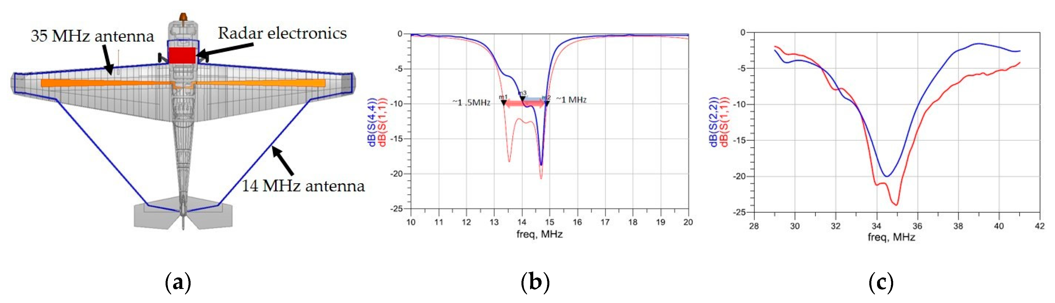
2.2.1. Platform and Antenna

The de Havilland Twin Otter is a twin turboprop aircraft with a cruise speed of 60 m/s and range of 1445 km [55]. The aircraft can be configured with either standard landing gear or skis, and it is well suited for low-altitude surveying of ice sheets. One of the biggest challenges in integrating the HF sounder on both the TO and the UAS is the size of the antenna elements (~5 m at 30 MHz). As shown in Figure 3, the antenna for the HF sounder consists of a single dipole element (designed to resonate at ~30 MHz) integrated into the tail tie down tube of the Norlandair Twin Otter. The available mounting supports on the aircraft were a limiting factor during the process of sizing and tuning the antenna to resonate at the desired frequency, particularly for the Band 1 mode. Thus, two lumped-element impedance matching networks (MN) were designed to enable dual frequency operation and improve the antenna bandwidth. The return loss of the antenna with and without the two matching networks is shown in Figure 4. The blue line is the antenna response with the Band 1 MN that results in a 1.1 MHz 6-dB bandwidth. The red line is the response with the Band 2 MN. The Band 2 MN increases the 8-dB bandwidth from 5 MHz to 11 MHz. We operated with 8 MHz on Band 2 to exploit the deep null at 31.5 MHz in the antenna response. The system was not configured to operate simultaneously in Band 1 and Band 2 during this field campaign.

2.2.2. Field Deployment

Certification flights and system tests were conducted over the Hofsjökull ice cap in Iceland and a transit over Greenland on 1 and 2 November 2016, respectively. Two 5 km flight lines over Hofsjökull were identified and flown five times each at an altitude of 400–450 m above the surface of the ice cap caldera. Ice thickness in this area was expected to be 100–800 m thick. Between the ice cap survey and transit flights, a total of 862 GB of data were collected.

The primary science target during the TO deployment was Jakobshavn Isbræ located on the west coast of Greenland approximately 60 km east of Ilulissat. Figure 5 shows the as-flown lines. We also collected data over the Greenland ice sheet during transits from and to Iceland. A key aspect of this field campaign was to fly repeat tracks with close spacing (approximately a quarter-wavelength of operating frequencies) to enable synthesizing large arrays in the cross-track direction, which can potentially improve clutter reduction. Over the course of four flight days, 11 lines along Jakobshavn Isbræ were flown—five in the middle (orange in Figure 5), three north of the middle line (blue), and three south of the middle line (red). Each line was repeated five times for a total of 55 passes. In addition, five cross lines were surveyed (blue). The total data volume collected during the survey was 2.42 TB.

2.3. Unmanned Aircraft System (UAS)

2.3.1. Platform

The G1X UAS (developed by the University of Kansas) is based on a subscale version of the YAK-54 aerobatic aircraft, which was formerly commercially available as a kit. The G1X has been modified to allow carriage of scientific payloads and increased fuel loads with a takeoff weight of 34 kg. An initial version of the G1X platform was documented in Leuschen et al. [51], and

Table 3. G1X Specifications.

Length		3 m
Wingspan		4.4 m
Engine		DA 120
Mass	empty	26 kg
	payload	3 kg
	batteries	2.5 kg
	fuel	2.5 kg
	max takeoff	34 kg
Speed	cruise	35 m/s
	stall	11 m/s
Range		160 km
Endurance		75 min
Landing distance	grass	50 m
	ice	90 m
	snow	75 m

provides a summary of vehicle details. Between the initial field deployment to subglacial Lake Whillans, Antarctica, in 2013 and the subsequent deployment to Russell Glacier, Greenland in 2016, we improved the vehicle’s performance and ruggedness for operations in the extreme polar environments. To accommodate the higher takeoff weight and improve the dynamic characteristics of G1X, the stock wingspan of 3.4 m was extended a total of 50 cm, including a 20 cm winglet with 45° dihedral angle. The spiral mode of the original G1X had a poor handling quality rating (Level III), making for difficult and unsafe landings in a cross-wind with high bank angles. The addition of winglets improved the wing loading of the G1X and the aircraft spiral mode handling quality to Level I.

To support payload power requirements, battery power was used to avoid electromagnetic interference with the radar. To ensure a continuous power supply for the payload, pairs of 28-volt batteries in parallel were used with diode protection to prevent one battery failure from impacting the other. Due to the ambient temperatures (as low as −26 °C), batteries were exchanged for fully-charged batteries while the fuel tanks were refilled after each flight.

2.3.2. Antenna

Unlike the Twin Otter, the G1X has two separate antennas to support the dual-band operation. As shown in Figure 6a, both antennas are integrated along the wing. The 35 MHz antenna is a tapered dipole antenna that is constructed from copper tape. The 14 MHz is a resistively-loaded dipole that is constructed from copper tape along the wing and horizontal tail which are connected with removable wires. Both antennas utilize a balun and separate impedance-matching networks. Figure 6b,c show the simulated and in-flight measured responses for the 14 MHz and 35 MHz antenna, respectively. Differences between the simulated and measured responses are attributed to the near proximity of the vehicle servo wiring and the in-flight dynamics [56].

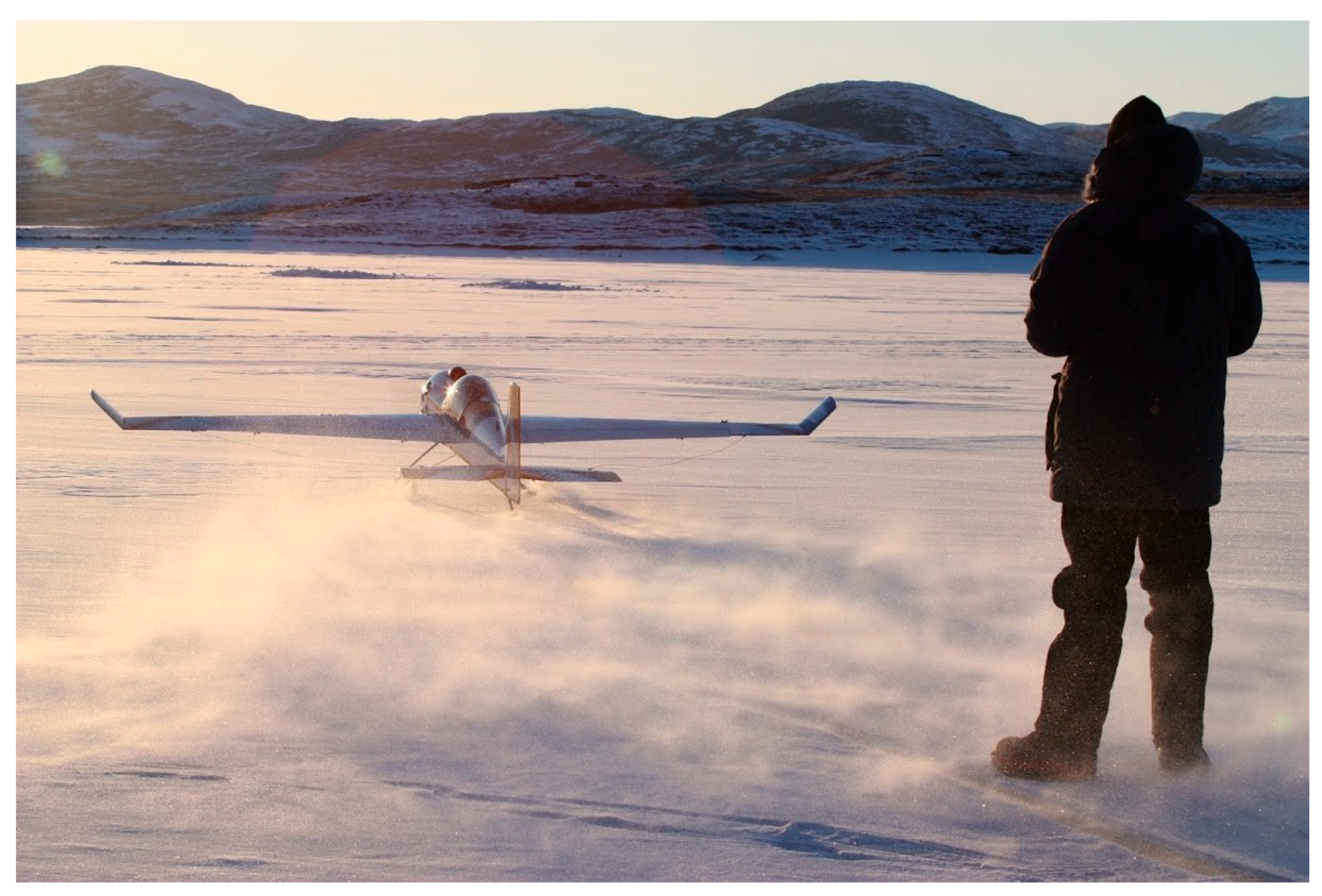
2.3.3. Field Deployment

During the Spring 2016 deployment to Greenland, all operations were based from a frozen lake (Lat: 67°5′38.43″ N and Lon: 50°16′46.14″ W) as shown in Figure 7. Surface conditions varied from a rough ice surface (requiring standard rubber tires) to a glass-like surface (requiring studded tires to maintain directional control on takeoff and landing) to a snow-covered surface (requiring skis). We conducted a total of 46 flights over Russell Glacier, 40 of which included autonomous flight segments. These flights represented over 40 hours of flight and 430 km over the horizon and glacier.

All data were collected with the radar operating in the 35 MHz mode. The vehicle was flown over three flight lines previously flown by the OIB VHF (MCoRDS) radar depth sounder installed on the NASA P-3. The three flight lines, shown in Figure 8, were characterized as “good,” “medium,” or “bad” quality, based on the discernibility of the ice bottom interface from the VHF radar data.

Several factors resulted in limited flight operations. Takeoffs and landings were conducted within 50 m of a steep 100 m high ridge immediately adjacent to the frozen lake. The presence of the ridge resulted in an asymmetrical field of view, and the lack of a uniform “horizon” contributed to the difficulties of operating in the extreme environment. Since UAS operations at Russell Glacier were only 19 km from Kangerlussauaq International Airport, the deployment team had to coordinate with air traffic control regularly. On many days, air traffic allowed a flight window of only one hour. Still, the biggest impediment to flying was the presence of high winds, especially late in the deployment. During one week, the team could not fly for six straight days due to winds as high as 25–28 m/s and record-setting warm temperatures.

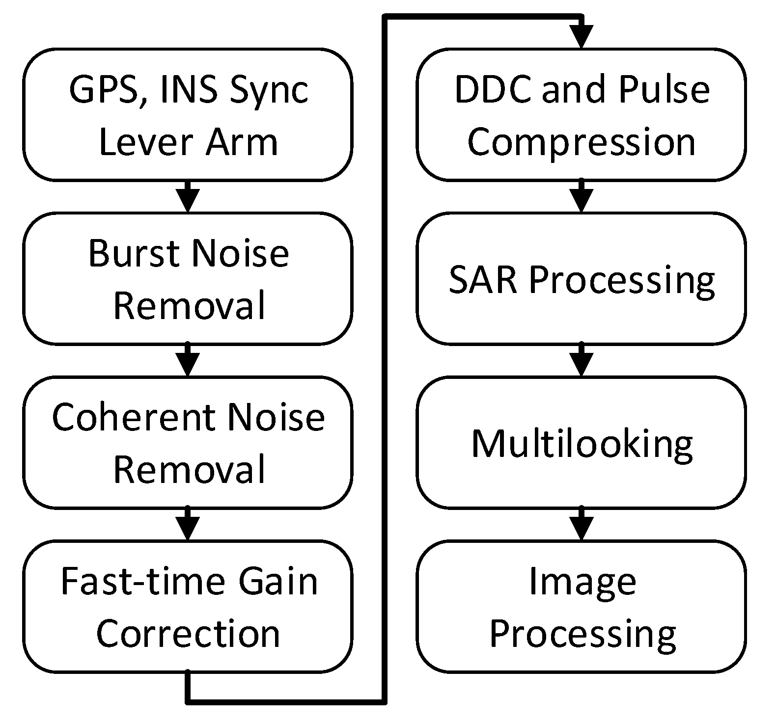
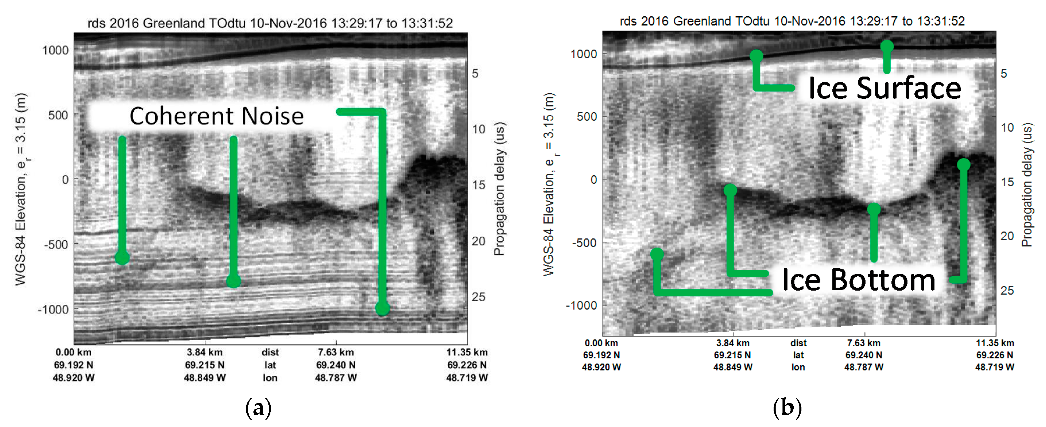
2.4. Data Processing

SAR echogram formation follows the data processing steps outlined in [58], although the bursty noise, coherent noise, and image-processing steps have been modified for the HF sounder data. Figure 9 illustrates the steps of the processing flow, including: metadata synchronization, noise removal, pulse compression, synthetic aperture radar processing, multilooking, and image processing for optimal viewing. The first step synchronizes the GPS and inertial measurement unit (IMU) data with the radar data and compensates for the lever arm between the GPS antenna and the radar antenna phase center. The radar antenna phase center is used in SAR processing and displays data relative to the WGS-84 ellipsoid. The remaining steps operate on radar data as described below.

Due to occasional recording errors, the stored data contain occasional spikes many orders of magnitude larger than the surrounding pixels. The bursty noise removal step identifies and removes these spikes. The removal process identifies the noisy pixels by applying a constant false alarm rate (CFAR) detector in the along-track dimension. The noise floor is estimated using a 22 tap filter with equal weights—11 taps before and 11 taps after the tested pixel. If the pixels exceed the background noise estimate by 20 dB, it is detected as a burst and set to zero. The along-track dimension is used because the range dimension contains abrupt changes in power due to direct feed through from the transmitter to receiver, the surface return, and the blanking switch. These abrupt changes are more difficult to account for when estimating the background noise for the CFAR detector.

The recorded data had a significant coherent noise source attributed to transients caused by the interaction between the antennas and the radar’s RF section. Coherent noise is unwanted signals containing amplitudes and phases that are predictable from pulse to pulse. Although the digital acquisition system employs zero-pi modulation [59], the recorded data still contain some residual coherent noise. In our case, the coherent noise is band limited to about 5 millihertz and centered on DC (zero frequency). The coherent noise is often much weaker than the desired scattering signal; if ordinary discrete Fourier transform (DFT) methods are used to estimate the low frequency coherent noise component, the estimate will be contaminated by the scattering signal. A user-defined threshold is used to exclude large scattering signals. The DFT is the application of the inner product to a sequence of basis vectors at different frequencies, so we modified its application by ignoring the basis vector elements that align with these excluded signals. The resulting basis vectors are re-normalized to account for the missing elements so the length of the new basis vectors is still one. The resulting DFT vectors are no longer orthogonal to each other. To account for this, we apply the inner products sequentially by projecting the data orthogonally to each steering vector after the inner product is found and using it for the next inner product.

After coherent noise removal, we convert the ADC quantized samples to voltage at the receiver input, which includes receiver gain compensation. Since the HF sounder operated with a fixed gain setting throughout each data collection segment, this step does not affect the echograms presented in Section 3 since these are all displayed on a relative scale.

During pulse compression, digital down conversion (DDC) is employed to bring the signal to complex baseband and then decimated with a poly-phase anti-aliasing filter. A matched filter is applied in the frequency domain [60]. The time domain representation of the matched filter signal is an ideal chirp weighted by a Tukey weighting matching that of the transmission:

$$s_{matched}\left(t\right)={\mathrm{tukey}}_{{\alpha }_{tukey}}\left(\frac{t}{T_{pd}}-0.5\right)\exp \left(j2\pi f_{0}t+j\pi \alpha t^2\right)$$

(3)

where $t$ is fast-time with the origin at the beginning of the transmission, ${\mathrm{tukey}}_{{\alpha }_{tukey}}$ is a tukey window with weight $0\le {\alpha }_{tukey}\le 1$, $T_{pd}$ is the pulse duration, $f_0$ is the start frequency, $\alpha =f_1-f_0/T_{pd}$ is the chirp rate, and $f_1$ is the stop frequency. The matched filter also includes a Hanning frequency domain window and sufficient zero-padding to prevent circular convolution.

Table 4. Signal transmission and processing settings.

Parameter	CReSIS G1XB	TO HF	TO HF
		Greenland	Iceland
Pulse duration	320 ns	1 μs	1 μs
Tukey weight	1	0.15	0.2
Start frequency	35 MHz	27.5 MHz	24.9 MHz
Stop frequency	35 MHz	35.5 MHz	34.9 MHz
Hanning BW	10 MHz	8 MHz	10 MHz
Decimation	10 MSPS	12.5 MSPS	12.5 MSPS
Blanking Switch	No	Yes	No

gives the digital down conversion and matched filter coefficients used for the various data segments.

The frequency-wavenumber (or f-k migration algorithm) described in [61] is used to SAR process the data. After SAR processing, motion compensation in the squint direction is removed so that the SAR image represents the original phase center of the measurement. The data are then multilooked 11 times and decimated by six in the along-track direction. Range multilooking is not done due to the limited bandwidth and coarse range resolution. To reduce the dynamic range of the images displayed in this work, the average power profile is removed by estimating the average power in each range bin, manually smoothing this curve; then the smoothed curve is subtracted from each column. This is most useful in removing the gain change from the blanking switch. Next, the Matlab Mathworks [62] tonemap function is used to apply tone mapping which effectively increases the local dynamic range or contrast by dividing the image into tiles and adaptively equalizing the histogram of each tile. The default settings of four row and four column tiles per image are used.

3. Results

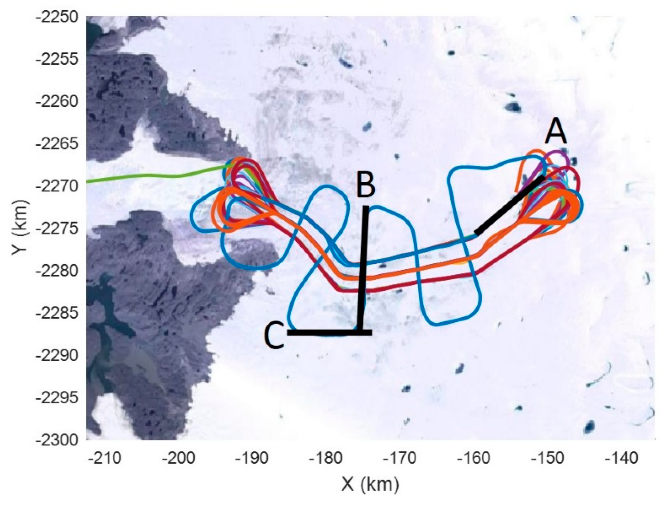
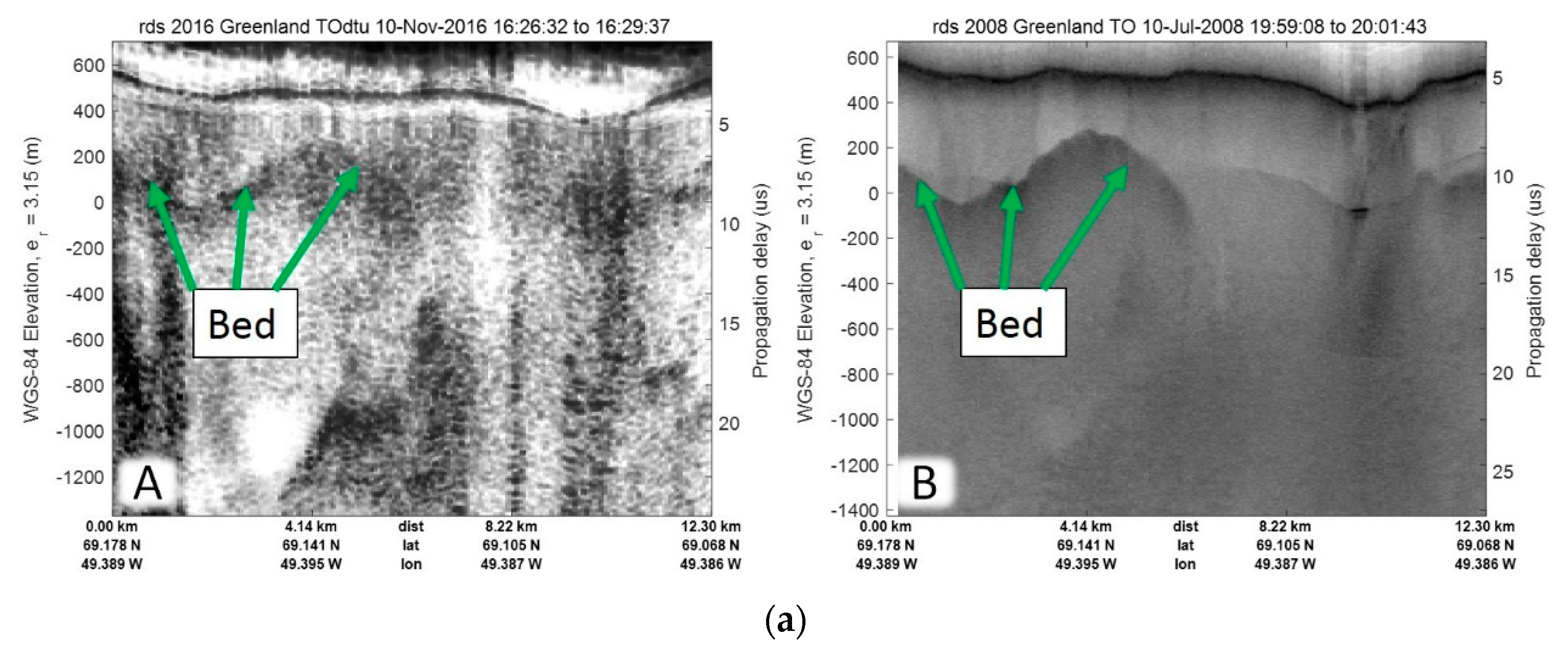
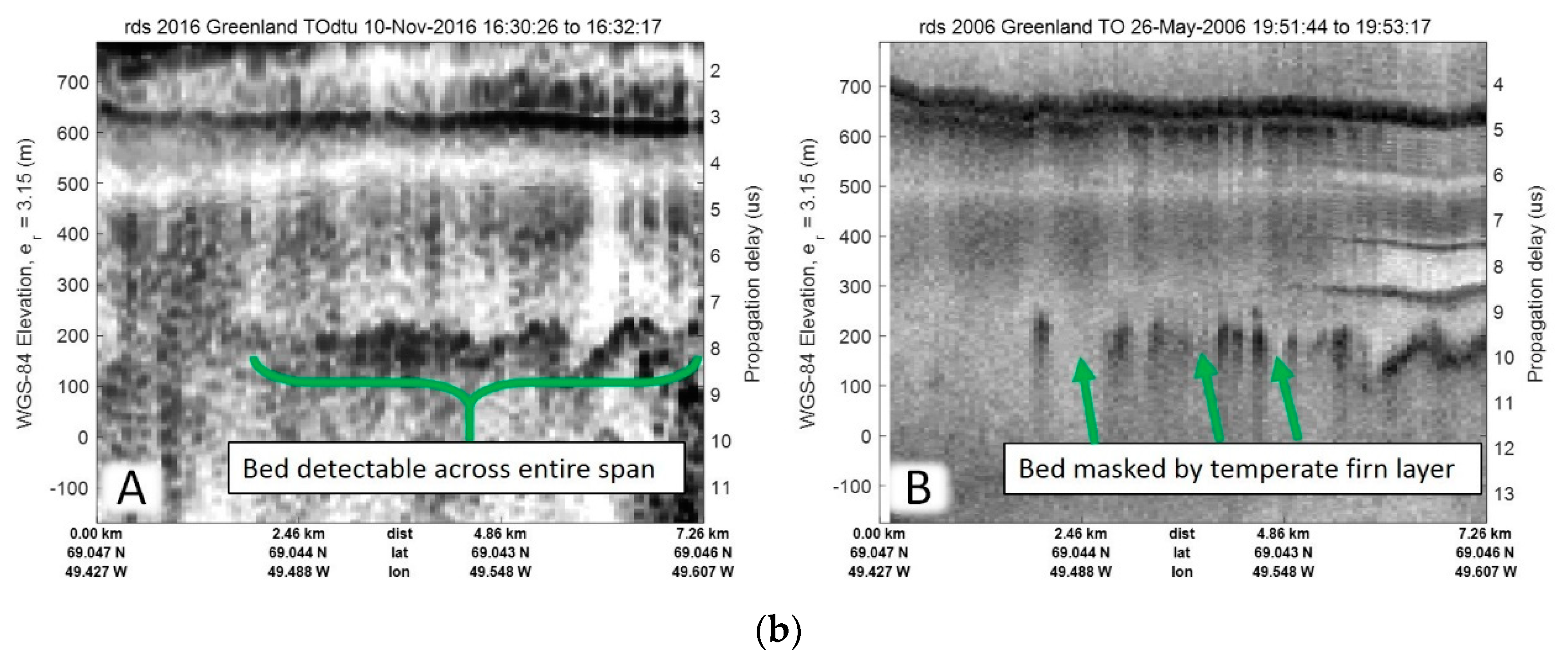
3.1. Twin Otter Results from the Jakobshavn Isbræ

Jakobshavn Isbræ is one of the most extensively studied glaciers due to its sudden acceleration and thinning over the last three decades [63,64]. However, this temperate, fast-flowing glacier is one of the most difficult targets to sound [65]. Figure 10 shows an echogram from the TO measurements over Jacobshavn Isbræ using the Band 2 mode. This echogram is from the northern side of the channel (marked as line segment A in Figure 5); the radar was able to detect the ice bottom across the entire 11 km stretch. Figure 10a shows the echogram prior to removing the coherent noise. In areas where the scattering signal was less than the coherent noise from the RF and antenna, the noise could be estimated and removed from all areas since it was stationary. Figure 10b shows the same echogram after the noise has been removed.

Various configurations of CReSIS MCoRDS radar have been flown over Jakobshavn during field campaigns since the 1990s. Figure 11 compares echograms produced by the HF sounder to those produced by the VHF sounder during campaigns in 2008 [66] and 2006 [67]. The MCoRDS VHF sounder images use the full antenna array (six elements in 2008 and five elements in 2006) and operated with 20 MHz bandwidth at a center frequency of 150 MHz. In both data sets, there is good agreement between the two radars when both detect the ice bottom. The two systems largely demonstrated similar detection capabilities in spite of the HF sounder being a single antenna system. The VHF system has improved surface clutter rejection (due to the electrically larger antenna aperture), while the HF sounder has improved penetration through temperate ice. The MCoRDS VHF sounder’s improved clutter rejection is illustrated in Figure 11a, where the edge of the channel is clear. In this same region of the HF sounder image, it is obscured by clutter. In addition, the HF sounder echogram in inset Figure 11b has some noted improvement over the VHF echogram. There are a few instances in the VHF echogram (right image) where the bed was not detected due to the temperate firn layer [66] but is detected in the HF echogram (left image).

To further emphasize the advantages of the multichannel VHF system, Figure 12 shows the same data from Figure 11a, but processed with only one channel. In this figure, the bed is completely undetectable, which clearly illustrates the decreased sensitivity of the HF sounder to scattering. These results strongly suggest the potential to further improve the HF sounder data if a cross-track array is synthesized. This 2D array synthesis could reduce off-angle clutter in areas where clutter is known to be the limiting factor [65].

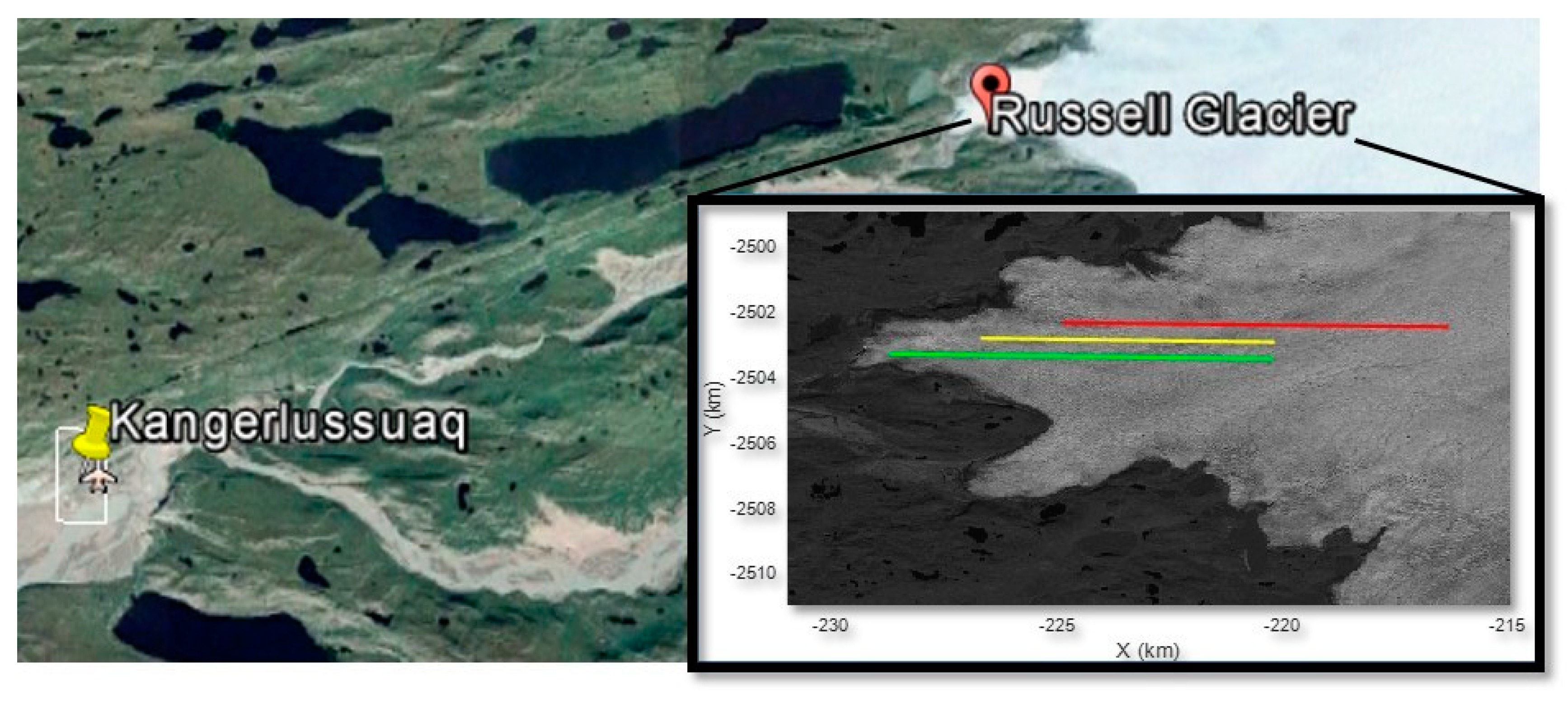
3.2. UAS Results from Russell Glacier

Figure 13 compares echograms produced from the HF sounder data during the April 2016 UAS deployment to those produced from the 195 MHz MCoRDS sounder data [25] during the April 2011 OIB deployment. These were repeat flights within a few tens of meters designed for the purpose of providing a direct comparison between the systems. The comparison of the TO HF sounder and the MCoRDS VHF sounder illustrates comparable performances over Jacobshavn (where the two-way attenuation rate has been estimated to be between 38–70 dB/km [65]). However, the UAS data set shows remarkable improvement over Russell Glacier, where the loss for the 500-m thick ice is estimated to be approximately 20 dB. As shown in Figure 13, the HF sounder identified 100% of the ice bottom along each flight track, but the bed is missing in some areas of the OIB data—even for the line labeled as “good.” The HF sounder was able to detect the bed consistently because of its reduced surface and volumetric scattering, and reduced signal extinction (compared to the higher frequency VHF system). This constitutes a significant improvement over the VHF sounder’s inconsistency in detecting ice bottoms. When the HF sounder and MCoRDS both identified the bottom, the thickness measurements agree very well.

To better quantify the improved detection capabilities of the HF sounder in this region, Figure 14 show SINR comparison plots for the bed signals in Figure 13. The interference and noise power were estimated by taking the mean power in a window of points before and after the peak. The duration of each window is 0.33 us, with the edge of each window starting 0.33 us away from the peak. The signal was estimated by taking the peak value at the bed and then subtracting the estimate of the interference and noise power. In the large gaps in the plots, the ice bottom is not detected in the MCoRDS image. Ice bottom pixels with a calculated SINR below −3 dB are also considered undetectable. The percentages of missed detections and mean SINR for each radar are included in the echograms. As the plots illustrate, in all cases the HF sounder had a higher detection rate and greater than 3 dB improvement in average SINR.

The same HF sounder flight lines crossed over measurements made in March 2010 with JPL’s WISE radar [49]. Although the WISE data were collected in 2010, repeat pass comparisons between April 2011 and April 2016 with the MCoRDS system showed no change in the signal extinction, indicating that this region seems to be temporally stable. Figure 15 shows the WISE data with three G1X crossover lines overlaid on the echograms. These are the same lines presented in Figure 8 and Figure 13; the WISE flight line is the blue vertical line on the HF sounder echograms in Figure 13a,c,e. In Figure 15, the ice surface and bottom detected by the CReSIS HF sounder are indicated by “x” marks. In the magnified region near the ice bottom (Figure 15b), it is clear that the ice bottom is largely not detected by the WISE data. Comparing Figure 13 with Figure 15 shows the improved performance of the CReSIS HF sounder over the WISE sounder.

We can attribute this improvement to a combination of factors, including: the stable antenna phase center (which improves SAR processing), slight SINR improvement due to the antenna orientation, as well as slight improvements in range resolution and accuracy. Range resolution, R, is the ability to discern closely spaced objects, and it is related to bandwidth (BW), speed of light (c), and the relative permittivity of the medium ε_r by R = (c/2B√ ε_r). The reported bandwidth of the WISE radar is between 1–3 MHz [49]. Compared to the 5 MHz bandwidth of the UAS HF Sounder, there is a 68–11 m decrease in range (vertical) resolution. Similarly, range measurement accuracy is proportional to range resolution. Assuming all other factors are constant, the larger bandwidth of the HF sounder would reduce uncertainty by a factor of 1.7–5. All of these factors contribute to the detectability of the bed.

Finally, we have also begun assessing the coherency of the return signals from multiple passes, as this is the first step in realizing 2D synthetic aperture capabilities. We completed co-registering adjacent passes (i.e., aligning adjacent flight lines). Figure 16a shows the phase map of the interferogram formed from two overlapping flight lines. The interferogram has been multilooked with a length 11 moving average filter in the along-track direction. The bright ice surface and bottom responses are phase coherent and stand out from the incoherent noisy background (black). The surface and bedrock returns come from the nadir direction and, as expected, the phase is nearly constant at 0°. Due to the uneven crevassed surface, topography, and noise, the phase angle from the ice surface and bottom are expected to have some variation about zero. The interferogram coherence (Figure 16b) provides a measure of the phase consistency between pixels. As expected the ice surface and bottom have high coherence.

4. Discussion

The sounding results presented here illustrate the promise of radars operating at high HF (14 MHz)/low VHF (30–35 MHz) for sounding temperate glaciers. This is particularly clear in areas like the Russell Glacier, where surface clutter is low enough that improved HF penetration allowed the ice bottom to be detected with even a single antenna system. For glaciers like Jakobshavn, the reduced signal extinction at low frequencies is offset by the difficulty in forming a large cross track aperture to suppress the surface clutter (although we are actively working on multipass processing to address this). As compared to other airborne radio echo sounders used for ice sheet measurements, this range of frequencies offers a good trade-off. The HF Sounder is inherently less sensitive to volume scatter and warm-ice attenuation compared to higher frequency VHF radars (150 and 195 MHz). On the other hand, the smaller antenna aperture is easier to integrate onto aircraft of various sizes (as compared to radars with lower operating frequencies), providing a stable phase center. The antenna response will improve SINR, as antenna patterns are important to signal coherence and the ability to model and reject clutter.

The incremental improvements of the HF sounder over Jakobshavn suggest that surface/volume clutter is still a major impediment at ~30 MHz. For future campaigns, one of our priorities will focus on data collection with the Band 1 mode. However, the multi-pass processing currently under development may improve the bed-detection capabilities of the HF sounder, especially in areas where detection capabilities are limited by off-nadir clutter. The initial coherency assessment between the multiple flight lines presented in Section 3.2 suggests 2D synthetic aperture processing may be possible through the use of multiple closely spaced flight lines. Due to their improved flight-tracking capabilities, UAS are the preferred platforms for such missions.

References

1. Meier, M.F. Contributions of Small Glaciers to Global Sea Level. Science 1984, 226, 1418–1421. [Google Scholar] [CrossRef] [PubMed]
2. Intergovernmental Panel on Climate Change (IPCC). 2013: Climate Change 2013: The Physical Science Basis. Contribution of Working Group I to the Fifth Assessment Report of the Intergovernmental Panel on Climate Change; Stocker, T.F., Qin, D., Plattner, G.-K., Tignor, M., Allen, S.K., Boschung, J., Nauels, A., Xia, Y., Bex, V., Midgley, P.M., Eds.; Cambridge University Press: Cambridge, UK; New York, NY, USA, 2013; 1535p. [Google Scholar]
3. Joughin, I.; Howat, I.M.; Fahnestock, M.; Smith, B.; Krabill, W.; Alley, R.B.; Stern, H.; Truffer, M. Continued Evolution of Jakobshavn Isbrae following Its Rapid Speedup. J. Geophys. Res. 2008, 113. [Google Scholar] [CrossRef]
4. Thomas, R.; Frederick, E.; Li, J.; Krabill, W.; Manizade, S.; Paden, J.; Sonntag, J.; Swift, R.; Yungel, J. Accelerating Ice Loss for the Fastest Greenland and Antarctic Glaciers. Geophys. Res. Lett. 2011, 38. [Google Scholar] [CrossRef]
5. Overpeck, J.T.; Otto-Bliesner, B.L.; Miller, G.H.; Muhs, D.R.; Alley, R.B.; Kiehl, J.T. Paleoclimatic Evidence for Future Ice-Sheet Instability and Rapid Sea-Level Rise. Science 2006, 311, 1747–1750. [Google Scholar] [CrossRef] [PubMed]
6. Anthoff, D.; Nicholls, R.J.; Tol, R.S.J.; Vafeidis, A.T. Global and Regional Exposure to Large Rises in Sea-Level: A Sensitivity Analysis; Working Paper 96; Tyndall Centre for Climate Change Research: Norwich, UK, 2006; p. 31. [Google Scholar]
7. Jacob, T.; Wahr, J.; Pfeffer, W.T.; Swenson, S. Recent contributions of glaciers and ice caps to sea level rise. Nature 2012, 482, 514–518. [Google Scholar] [CrossRef] [PubMed]
8. Larour, E.; Schiemrmeier, J.; Rignot, E.; Seroussi, H.; Morlighem, M.; Paden, J. Sensitivity Analysis of Pine Island Glacier Ice Flow using ISSM and Dakota. J. Geophys. Res. 2012, 117. [Google Scholar] [CrossRef]
9. Legarsky, J.; Gogineni, S. Unfocused SAR using a Next-Generation COoherent Radar Depth Sounder for measurement of Greenland ice sheet thickness. IGARSS 1998, 1, 463–465. [Google Scholar] [CrossRef]
10. Gogineni, S.; Chuah, T.S.; Allen, C.; Jezek, K.; Moore, R.K. An improved coherent radar depth sounder. J. Glaciol. 1998, 44, 659–669. [Google Scholar] [CrossRef]
11. Gogineni, S.; Tammana, D.; Braaten, D.; Leuschen, C.; Akins, T.; Legarsky, J.; Kanagaratnam, P.; Stiles, J.; Allen, C.; Jezek, K. Coherent radar ice thickness measurements over the Greenland ice sheet. J. Geophys. Res. 2001, 106, 33761–33772. [Google Scholar] [CrossRef]
12. Jezek, K.; Wu, X.; Gogineni, S.; Rodriguez, E.; Freeman, A.; Rodriguez-Morales, F.; Clark, C. Radar Images of the bed of the Greenland ice sheet. Geophys. Res. Lett. 2011, 38. [Google Scholar] [CrossRef]
13. Li, J.; Paden, J.; Leuschen, C.; Rodriguez-Morales, F.; Hale, R.; Arnold, E.; Crowe, R.; Gomez-Garcia, D.; Gogineni, S. High-altitude radar measurements of ice thickness over the Antarctic and Greenland ice sheets as part of Operation Ice Bridge. IEEE Trans. Geosci. Remote Sens. 2013, 51, 742–754. [Google Scholar] [CrossRef]
14. Panzer, B.; Gomez-Garcia, D.; Leuschen, C.; Paden, J.; Rodriguez-Morales, F.; Patel, A.; Markus, T.; Holt, B.; Gogineni, P. An ultra-wideband, microwave radar for measuring snow thickness on sea ice and mapping near-surface internal layers in polar firn. J. Glaciol. 2013, 59, 244–254. [Google Scholar] [CrossRef]
15. Yan, J.-B.; Gomez-Garcia, D.; McDaniel, J.W.; Li, Y.; Gogineni, S.; Rodriguez-Morales, F.; Brozena, J.; Leuschen, C.J. Ultrawideband FMCW radar for airborne measurements of snow over sea ice and land. IEEE Trans. Geosci. Reomote Sens. 2017, 55, 834–843. [Google Scholar] [CrossRef]
16. MacGregor, J.A.; Fahnestock, M.A.; Catania, G.A.; Aschwanden, A.; Clow, G.D.; Colgan, W.T.; Gogineni, S.P.; Morlighem, M.; Nowicki, S.M.; Paden, J.D.; et al. A synthesis of the basal thermal state of the Greenland Ice Sheet. J. Geophys. Res. Earth Surf. 2016, 121, 1328–1350. [Google Scholar] [CrossRef] [PubMed]
17. Oswald, G.K.A.; Gogineni, S.P. Recovery of subglacial water extent from Greenland radar survey data. J. Glaciol. 2008, 54, 94–106. [Google Scholar] [CrossRef]
18. Oswald, G.K.A.; Gogineni, S.P. Mapping basal melt under the northern Greenland Ice Sheet. IEEE Trans. Geosci. Remote Sens. 2012, 50, 585–592. [Google Scholar] [CrossRef]
19. MacGregor, J.A.; Fahnestock, M.A.; Catania, G.A.; Paden, J.D.; Gogineni, S.P.; Young, S.K.; Rybarski, S.C.; Mabrey, A.N.; Wagman, B.M.; Morlighem, M. Radiostratigraphy and age structure of the Greenland Ice Sheet. J. Geophys. Res. Earth Surf. 2015, 120, 212–241. [Google Scholar] [CrossRef] [PubMed]
20. Jordan, T.M.; Cooper, M.A.; Schroeder, D.M.; Williams, C.N.; Paden, J.D.; Siegert, M.J.; Bamber, J.L. Self-affine subglacial roughness: Consequences for radar scattering and basal water discrimination in northern Greenland. Cryosphere 2017, 11, 1247–1264. [Google Scholar] [CrossRef]
21. Thomas, R.H. Program for Arctic Regional Climate Assessment (PARCA): Goals, key findings, and future directions. J. Geophys. Res. 2001, 106, 33691–33706. [Google Scholar] [CrossRef]
22. Studinger, M.; Koenig, L.; Martin, S.; Sonntag, J.G. Operation Icebridge: Using instrumented aircraft to bridge the observational gap between ICESat and ICESat-2. In Proceedings of the 2010 IEEE International Geoscience and Remote Sensing Symposium (IGARSS), Honolulu, HI, USA, 25–30 July 2010. [Google Scholar]
23. Bamber, L.J.; Griggs, J.A.; Hurkmans, R.T.W.L.; Dowdeswell, J.A.; Gogineni, S.P.; Howat, I.; Mouginot, J.; Paden, J.; Palmer, S.; Rignot, E.; et al. A New Bed Elevation Dataset for Greenland. Cryosphere 2013, 7, 499–510. [Google Scholar] [CrossRef]
24. Fretwell, P.; Pritchard, H.D.; Vaughan, D.G.; Bamber, J.L.; Barrand, N.E.; Bell, R.; Bianchi, C.; Bingham, R.G.; Blankenship, D.D.; Casassa, G.; et al. Bedmap2: Improved Ice Bed, Surface and Thickness Datasets for Antarctica. Cryosphere 2013, 7, 375–393. [Google Scholar] [CrossRef] [Green Version]
25. Rodriguez-Morales, F.; Gogineni, S.; Leuschen, C.J.; Paden, J.D.; Li, J.; Lewis, C.C.; Panzer, B.; Alvestegui, D.G.G.; Patel, A.; Byers, K.; et al. Advanced Multi-Frequency Radar Instrumentation for Polar Research. IEEE Trans. Geosci. Remote Sens. 2014, 52, 2824–2842. [Google Scholar] [CrossRef]
26. Nixdorf, U.; Steinhage, D.; Meyer, U.; Hempel, L.; Jenett, M.; Wachs, P.; Miller, H. The newly developed airborne radio-echo sounding system of the AWI as a glaciological tool. Ann. Glaciol. 1999, 29, 231–238. [Google Scholar] [CrossRef]
27. Corr, H.; Ferraccioli, F.; Frearson, N.; Jordan, T.; Robinson, C.; Armadillo, E.; Caneva, G.; Bozzo, E.; Tabacco, I. Airborne radio-echo sounding of the Wilkes subglacial basin, the Transantarctic Mountains, and the Dome C region. Terra Antarct. Rep. 2007, 13, 55–64. [Google Scholar]
28. Rippin, D.M.; Vaughan, D.G.; Corr, H.F.J. The basal roughness of Pine Island Glacier, west Antarctica. J. Glaciol. 2011, 57, 67–76. [Google Scholar] [CrossRef]
29. Vaughan, D.G.; Corr, H.F.J.; Ferraccioli, F.; Frearson, N.; O’Hare, A.; Mach, D.; Holt, J.W.; Blankenship, D.D.; Morse, D.L.; Young, D.A. New boundary conditions for the West Antarctic ice sheet: Subglacial topography beneath Pine Island Glacier. Geophys. Res. Lett. 2006, 33, 33. [Google Scholar] [CrossRef]
30. Lindbäck, K.; Pettersson, R.; Doyle, S.H.; Helanow, C.; Jansson, P.; Kristensen, S.S.; Stenseng, L.; Forsberg, R.; Hubbard, A.L. High-resolution ice thickness and bed topography of a land-terminating section of the Greenland ice sheet. Earth Syst. Sci. Data 2014, 6, 331–338. [Google Scholar] [CrossRef] [Green Version]
31. Peters, M.; Blankenship, D.D.; Carter, S.P.; Kempf, S.D.; Young, D.A.; Holt, J.W. Along-track focusing of airborne radar sounding dada from Wes Antarctica for improving basal reflection analysis and layer detection. IEEE Trans. Geos. Remote Sens. 2007, 45, 2725–2736. [Google Scholar] [CrossRef]
32. Peters, M.E.; Blankenship, D.D.; Morse, D.L. Analysis techniques for coherent airborne radar sounding: Application to West Antarctic ice streams. J. Geophys. Res. 2005, 110, B06303. [Google Scholar] [CrossRef]
33. Morlighem, M.; Williams, C.N.; Rignot, E.; An, L.; Arndt, J.E.; Bamber, J.L.; Catania, G.; Chauché, N.; Dowdeswell, J.A.; Dorschel, B.; et al. BedMachine v3: Complete Bed Topography and Ocean Bathymetry Mapping of GreenlandFrom Multibeam Echo Sounding Combined with Mass Conservation. Geophys. Res. Lett. 2017, 44, 11051–11061. [Google Scholar] [CrossRef] [PubMed]
34. Griggs, J.A.; Bamber, J.L. Antarctic Ice-Shelf Thickness from Satellite Radar Altimetry. J. Glaciol. 2011, 57, 485–498. [Google Scholar] [CrossRef]
35. Bamber, J.L.; Gomez-Dans, J.L.; Griggs, J.A. A New 1 km Digital Elevation Model of the Antarctic Derived from Combined Satellite Radar and Laser Data—Part 1: Data and Methods. Cryosphere 2009, 3, 101–111. [Google Scholar] [CrossRef] [Green Version]
36. Thomas, R.H. The dynamics of marine ice sheets. J. Glaciol. 1979, 24, 167–177. [Google Scholar] [CrossRef]
37. Watts, R.D.; Wright, D.L. Systems for measuring thickness of temperate and polar ice from the ground or from the air. J. Glaciol. 1981, 27, 459–469. [Google Scholar] [CrossRef]
38. Watts, R.D.; Wright, D.L. Radio-echo sounding of temperate glaciers: Ice properties and sounder design criteria. J. Glaciol. 1976, 17, 39–48. [Google Scholar] [CrossRef]
39. Smith, B.M.E.; Evans, S. Radio echo sounding: Absorption and scattering by water inclusion and ice lenses. J. Glaciol. 1972, 11, 133–146. [Google Scholar] [CrossRef]
40. Kong, A. Effective Permittivity for a Volume Scattering Medium in Electromagnetic Wave Theory; Wiley: New York, NY, USA, 1986; Chapter 6, Section 7; pp. 550–563. [Google Scholar]
41. Ishimaru, A. Wave Propagation and Scattering in Random Media; Academic: New York, NY, USA, 1978. [Google Scholar]
42. MacGregor, J.A.; Li, J.; Paden, J.D.; Catania, G.A.; Clow, G.D.; Fahnestock, M.A.; Gogineni, S.P.; Grimm, R.E.; Morlighem, M.; Nandi, S.; et al. Radar attenuation and temperature within the Greenland Ice Sheet. J. Geophys. Res. Earth Surf. 2015, 120, 983–1008. [Google Scholar] [CrossRef]
43. Jordan, T.M.; Bamber, J.L.; Williams, C.N.; Paden, J.D.; Siegert, M.J.; Huybrechts, P.; Gagliardini, O.; Gillet-Chaulet, F. An ice-sheet-wide framework for englacial attenuation from ice-penetrating radar data. Cryosphere 2016, 10, 1547–1570. [Google Scholar] [CrossRef] [Green Version]
44. Paden, J.D.; Allen, C.T.; Gogineni, S.; Jezek, K.C.; Dahl-Jensen, D.; Larsen, L.B. Wideband measurements of ice sheet attenuation and basal scattering. IEEE Geosci. Remote Sens. Lett. 2005, 2, 164–168. [Google Scholar] [CrossRef]
45. Brown, C.S.; Rasmussen, L.A.; Meier, M. Bed Topography Inferred from Airborne Radio-echo Sounding of Columbia Glacier, Alaska; U.S. Geological Survey Professional Paper; United States Government Printing Office: Washington, DC, USA, 1986; p. 1258-G.
46. Zamora, R.; Ulloa, D.; Garcia, G.; Mella, R.; Uribe, J.; Wendt, J.; Rivera, A.S.; Gacitua, G.; Casassa, G. Airborne radar sounder for temperate ice: Initial results from Patagonia. J. Glaciol. 2009, 55, 507–512. [Google Scholar] [CrossRef]
47. Blindow, N.; Salat, C.; Casassa, G. Airborne GPR sounding of deep temperate glaciers—Examples from the Northern Patagonian Icefield. In Proceedings of the 2012 14th International Conference on Ground Penetrating Radar (GPR), Shanghai, China, 4–8 June 2012; pp. 664–669. [Google Scholar]
48. Rignot, E.; Mouginot, J.; Larsen, C.F.; Gim, Y.; Kirchner, D. Low-frequency radar sounding of temperate ice masses in Southern Alaska. Geophys. Res. Lett. 2013, 40, 5399–5405. [Google Scholar] [CrossRef]
49. Mouginot, J.; Rignot, E.; Gim, Y.; Kirchner, D.; Le Meur, E. Low-Frequency Radar Sounding of Ice in East Antarctica and Southern Greenland. Ann. Glaciol. 2014, 55, 138–146. [Google Scholar] [CrossRef]
50. Conway, H.; Smith, B.; Vaswani, P.; Matsuoka, K.; Rignot, E.; Claus, P. A Low-Frequency Ice-Penetrating Radar System Adapted for Use from an Airplane: Test Results for Bering and Malaspina Glaciers, Alaska, USA. Ann. Glaciol. 2009, 50, 93–97. [Google Scholar] [CrossRef]
51. Recommendation ITU-R P.372-11. Radar Noise; International Telecommunication Union: Geneva, Switzerland, 2013. [Google Scholar]
52. Leuschen, C.; Hale, R.; Keshmiri, S.; Yan, J.-B.; Rodriguez-Morales, F.; Mahmood, A.; Gogineni, S. UAS-based Radar Sounding of the Polar Ice Sheets. IEEE Geosci. Remote Sens. Mag. 2014, 2, 8–17. [Google Scholar] [CrossRef]
53. Arcone, S.; Lawson, D.; Delaney, A.J.; Moran, M.L. 12–100 MHz depth and stratigraphic profiles of temperate glaciers. In Proceedings of the SPIE 4084, Eighth International Conference on Ground Penetrating Radar, Gold Coast, Australia, 23–26 April 2000; Volume 4084. [Google Scholar]
54. Rodriguez-Morales, F.; Gogineni, S.; Ahmed, F.; Carabajal, C.; Paden, A.; Leuschen, C.; Paden, J.; Li, J.; Fields, W.; Vaughan, J. High-Power, wideband transmit/receive switches and modules for ice sounding/imaging radar. Microw. J. 2016, 59, S6–S18. [Google Scholar]
55. DHC-6 Twin Otter. Jane’s All the World Aircraft, 1984–1985; Jane’s Publishing Incorporated: New York, NY, USA, 1985. [Google Scholar]
56. Mahmood, A. Design, Integration, and Deployment of UAS borne HF/VHF Depth Sounding Radar and Antenna System. Master’s Thesis, University of the Kansas, Lawrence, KS, USA, 2017. [Google Scholar]
57. Keshmiri, S.; Arnold, E.J.; Blevins, A.; Ewing, M.; Hale, R.; Leuschen, C.; Lyle, J.; Mahmood, A.; Paden, J.; Rodriquez-Morales, F.; et al. Radar Echo Sounding of Russell Glacier at 35 MHz Using Compact Radar Systems on Small Unmanned Aerial Vehicles. In Proceedings of the 2017 IEEE International Geoscience and Remote Sensing Symposium (IGARSS), Fort Worth, TX, USA, 23–28 July 2017. [Google Scholar]
58. Paden, J. Radar Depth Sounder. Available online: Ftp://data.cresis.ku.edu/data/rds/rds_readme.pdf (accessed on 13 April 2018).
59. Allen, C.T.; Mozaffar, S.N.; Akins, T.L. Suppressing Coherent Noise in Radar Applications with Long Dwell Times. IEEE Geosci. Remote Sens. Lett. 2005, 2, 284–286. [Google Scholar] [CrossRef]
60. Stimson, G.W. Airborne Radar; SciTech: Raleigh, NC, USA, 1998; pp. 317–322. [Google Scholar]
61. Leuschen, C.; Gogineni, P.; Tammana, D. SAR Processing of Radar Echo Sounder Data. In Proceedings of the IEEE 2000 International Geoscience and Remote Sensing Symposium, Honolulu, HI, USA, 24–28 July 2000. [Google Scholar] [CrossRef]
62. MATLAB 2017a; MathWorks Inc.: Natick, MA, USA, 2017.
63. Rignot, E.; Kanagaratnam, P. Changes in the Velocity Structure of the Greenland Ice Sheet. Science 2006, 311, 986–990. [Google Scholar] [CrossRef] [PubMed]
64. Holland, D.M.; Thomas, R.H.; Young, B.; Ribergaard, M.H.; Lyberth, B. Acceleration of Jakobshavn Isbrae triggered by warm subsurface ocean waters. Nat. Geosci. 2008, 1, 659–664. [Google Scholar] [CrossRef]
65. Gogineni, S.; Yan, J.B.; Paden, J.; Leuschen, C.; Li, J.; Rodriguez-Morales, F.; Braaten, D.; Purdon, K.; Wang, Z.; Liu, W.; et al. Bed topography of Jakobshavn Isbræ, Greenland, and Byrd Glacier, Antarctica. J. Glaciol. 2014, 60, 813–833. [Google Scholar] [CrossRef]
66. Marathe, K.C. Dual-Band Multi-Channel Airborne Radar for Mapping the Internal and Basal Layers of Polar Ice Sheets. Master’s Thesis, University of Kansas, Lawrence, KS, USA, 2008. [Google Scholar]
67. Lohoefener, A. Design and Development of a Multi-Channel Radar Depth Sounder. Master’s Thesis, University of Kansas, Lawrence, KS, USA, 2006. [Google Scholar]
68. Forster, R.R.; Box, J.E.; Van Den Broeke, M.R.; Miège, C.; Burgess, E.W.; Van Angelen, J.H.; Lenaerts, J.T.; Koenig, L.S.; Paden, J.; Lewis, C.; et al. Extensive liquid meltwater storage in firn within the Greenland ice sheet. Nat. Geosci. 2014, 7, 95–98. [Google Scholar] [CrossRef]
Figure 1. Long resistively loaded wire antenna concept used for other temperate ice sounders. The orientation of the dipole pattern will slightly degrade signal to interference and noise ratio (SINR).
Geosciences 08 00182 g001
Figure 2. Simplified block diagram of the CReSIS HF/VHF radar. This diagram represents both the TO and UAS version of the radar.
Geosciences 08 00182 g002
Figure 3. HF Sounder antenna and radar electronics installed on Norlandair Twin Otter.
Geosciences 08 00182 g003
Figure 4. Return loss of installed Twin Otter antenna with and without a matching network. Black is the antenna response, blue is the antenna response with the Band 1 MN, and red is the antenna response with the Band 2 MN.
Geosciences 08 00182 g004
Figure 5. Flight lines over Jakobshavn Glacier in Greenland. United States Geological Survey (USGS)/National Aeronautics and Space Administration (NASA) Landsat-7 imagery in background and National Snow and Ice Data Center (NSIDC) Arctic Polar Stereographic projection. Line segments A–C show the location of radar echogram figures.
Geosciences 08 00182 g005
Figure 6. G1X UAS antenna integration and installed measurement; (a) shows the antenna and radar electronic integration on the vehicle; (b) show the simulated (red) and in-flight measured (blue) response of the 14 MHz antenna; (c) is the simulated (red) and in-flight measured (blue) response of the 35 MHz antenna. © 2017 IEEE. Insets (b,c) reprinted, with permission, from [57].
Geosciences 08 00182 g006
Figure 7. UAS pilot taking off from a frozen lake near Russell Glacier, Greenland.
Geosciences 08 00182 g007
Figure 8. Proximity of Russell Glacier to Kangerlussuaq, Greenland (background from Google Earth). The inset image shows the flight lines used to compare the data from the HF sounder and the NASA Operation Ice Bridge (OIB) VHF depth sounder. The green, yellow and red lines represent “good,” “medium,” and “bad” quality data, respectively, from the OIB VHF sounder. Flight lines are overlaid on a Landsat-7 image.
Geosciences 08 00182 g008
Figure 9. Data-processing workflow.
Geosciences 08 00182 g009
Figure 10. Example radar echogram from the northern side of the Jakobshavn channel; corresponds to line segment A in Figure 5; (a) shows the echogram prior to the removal of the coherent noise and (b) is the echogram after the noise has been removed. (see Supplementray Materials).
Geosciences 08 00182 g010
Figure 11. Inset (a) is a comparison of the TO HF sounder Band 2 data (left) and MCoRDS VHF radar data (right) taken during 2008. These data sets were taken along line segment B in Figure 5; Inset (b) is a comparison of the HF sounder (left) and the VHF radar from 2006. This data corresponds to line C in Figure 5. Bed location agrees well in the two data sets. (see Supplementray Materials).
Geosciences 08 00182 g011aGeosciences 08 00182 g011b
Figure 12. Single channel MCoRDS data from Figure 11a. While the bed was partially detectable for the full array, it is not discernable for a single channel. (see Supplementray Materials).
Geosciences 08 00182 g012
Figure 13. Comparison of the HF sounder echograms (left) to the MCoRDS VHF sounder echograms (right). The “good quality” lines are presented in (a,b), the “medium quality lines are presented in (c,d), and the “poor” quality lines are presented in (e,f). As can be seen from the figures in the left column, the ice bottom is detected nearly 100% of the time along the flight line including in locations where MCoRDS did not detect the bottom. The blue vertical line represents the cross-over locations of the Jet Propulsion Laboratory (JPL) Warm Ice Sounding Explorer (WISE) radar. © 2017 IEEE. Reprinted, with permission, from [68]. (see Supplementray Materials).
Geosciences 08 00182 g013aGeosciences 08 00182 g013b
Figure 14. SINR Comparisons for the HF Sounder and MCoRDS echograms shown in Figure 13. Figures (ac) are the good, medium, and bad lines, respectively. The blue data is the HF sounder data, and the brown data is the MCoRDS data. (see Supplementray Materials).
Geosciences 08 00182 g014
Figure 15. (a) Comparison with WISE manned HF sounder data. The intersection with the G1X flight lines (same shown in Figure 6) are represented by the green, yellow, and red lines. The time tag for the WISE data is 20100318_14_001. The location of the ice surface and ice bottom detected by the CReSIS HF sounder is denoted with an ‘x’, and (b) the magnified region around the ice bottom shows that the WISE data quality is significantly lower than the HF sounder. © 2017 IEEE. Reprinted, with permission, from [57].
Geosciences 08 00182 g015
Figure 16. Phase coherence from co-registration of multiple passes. (a) Phase-angle map of the interferogram formed from two overlapping passes taken on two different flights. The interferogram angle is represented by the hue (color) and the log-magnitude is represented by the value (dark is low magnitude). The ice surface and ice bottom show good coherence whereas the background noise has poor coherence and the angle varies rapidly from pixel to pixel. (b) Interferogram coherence (1 represents perfect coherence). (see Supplementray Materials).
Geosciences 08 00182 g016