
Hydroacoustic Observations of Two Contrasted Seismic Swarms along the Southwest Indian Ridge in 2018


Laboratoire Geosciences Ocean, University of Brest & CNRS, 29280 Plouzané, France
*
Author to whom correspondence should be addressed.
Geosciences 2021, 11(6), 225; https://doi.org/10.3390/geosciences11060225
Submission received: 5 April 2021
/
Revised: 9 May 2021
/
Accepted: 18 May 2021
/
Published: 24 May 2021
(This article belongs to the Special Issue Earthquake Swarms)
Abstract
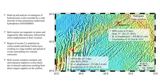
:In 2018, two earthquake swarms occurred along spreading ridge segments of the ultra-slow Southwest Indian Ridge (SWIR). The first swarm was located at the spreading-ridge intersection with the Novara Fracture Zone, comprising 231 events (ISC catalogue) and spanning over 6 days (10 July to 15 July). The second swarm was more of a cluster of events focusing near a discontinuity, 220 km west of the Rodrigues Triple Junction, composed of 92 events and spanning over 31 days (27 September to 27 October). We examined these two swarms using hydroacoustic records from the OHASISBIO network with seven to nine autonomous hydrophones moored on either side of the SWIR. We detected 1109 hydroacoustic events spanning over 13 days (6 July to 18 July) in the first swarm and 4880 events spanning over 33 days in the second swarm (25 September to 27 October). The number of events per day was larger, and the hydroacoustic magnitude (source level) was, on average, smaller during the second swarm than the first. The spatio-temporal distribution of events from both swarms indicates a magmatic origin initiated by dike intrusions and followed by a readjustment of stresses in the surrounding crust.
1. Introduction
Seismic swarms are sequences of earthquakes with no major mainshock. They do not have a well-defined temporal order in the magnitude of events and seismicity rate [1,2]. Seismic swarms at mid-ocean ridges have been investigated since the 1970s (e.g., [3,4,5,6,7,8]). Swarms of volcanic and tectonic events along mid-ocean ridges are inherent to seafloor spreading [9]. Because of the remoteness of most of the mid-ocean ridges and due to the rapid attenuation of seismic waves in the solid Earth, land-based seismic networks lack the low-level seismicity associated with seafloor spreading processes [10,11]. Since the late 1980s, local studies using ocean-bottom seismometers (OBS) (e.g., [12,13,14]) and regional studies using autonomous underwater hydrophones (AuH) (e.g., [15,16,17]) have greatly contributed to a detailed understanding of mid-ocean ridge seismicity [18,19,20]. This is possible because seismic events produce low-frequency hydroacoustic waves, known as T-waves, that are excited in the water column by earthquakes through the conversion of seismic waves into acoustic waves at the solid–liquid interface (i.e., sea-bottom) [10,15,20] and which propagate through the sound fixing and ranging (SOFAR) channel over long distances with little attenuation [21,22,23].
The Southwest Indian Ridge (SWIR) is a major seafloor spreading ridge separating Africa and Antarctica. It extends from the Bouvet Triple Junction in the southern Atlantic Ocean to the Rodrigues Triple Junction (RTJ) in the Indian Ocean [24,25,26]. The western end of SWIR is older than its eastern end due to the lengthening and eastward propagation of the ridge axis toward the RTJ [27,28]. The SWIR is among the world’s slowest spreading ridges, with a full spreading rate of ~14 mm/a [24,29,30]. It is also characterized by several large-offset transform faults that divide the ridge into spreading segments of various lengths [31,32] with several magmatic and amagmatic ridge segments [33] and a deep axial valley bounded by ~3 km high ridges [26,28,32]. The cyclic nature of volcanic construction and tectonic dismemberment across the SWIR is responsible for the ridge crests and rugged morphology of this spreading ridge [32]. As shown in Figure 1, the SWIR is mostly characterized by the obliquity of the ridge axis with respect to the main fracture zone’s (FZ) orientation [34,35]. The section of the ridge between the Gallieni (52° E) and Melville FZ (60° E) shows an obliquity of 40° and contains several long-lived transform and non-transform discontinuities. The section between Melville FZ and RTJ (70° E) has an obliquity of 25° and is continuous with minor discontinuities.
Only a few seismic swarms have been reported along the SWIR based on teleseismic observations (e.g., [36,37]), hydroacoustic observations (e.g., [38,39]) or local OBS surveys (e.g., [40,41]). In a comprehensive study of teleseismic earthquakes between 1976 and 2010 at ultra-slow spreading ridges, Schlindwein [42] showed that earthquake swarms occur at volcanic centers or segments with magmatic accretion that are separated by stretches of non-volcanic seafloor. These swarms are mostly associated with diking events. In the western part of the SWIR, based on regional and teleseismic earthquakes, Läderach et al. [43] showed that earthquake swarms are associated with along-axis melt flow mechanisms. Seismic swarms observed in local OBS studies in the eastern part of the SWIR are also interpreted as the result of magma movement related to diking episodes [7,40,44].
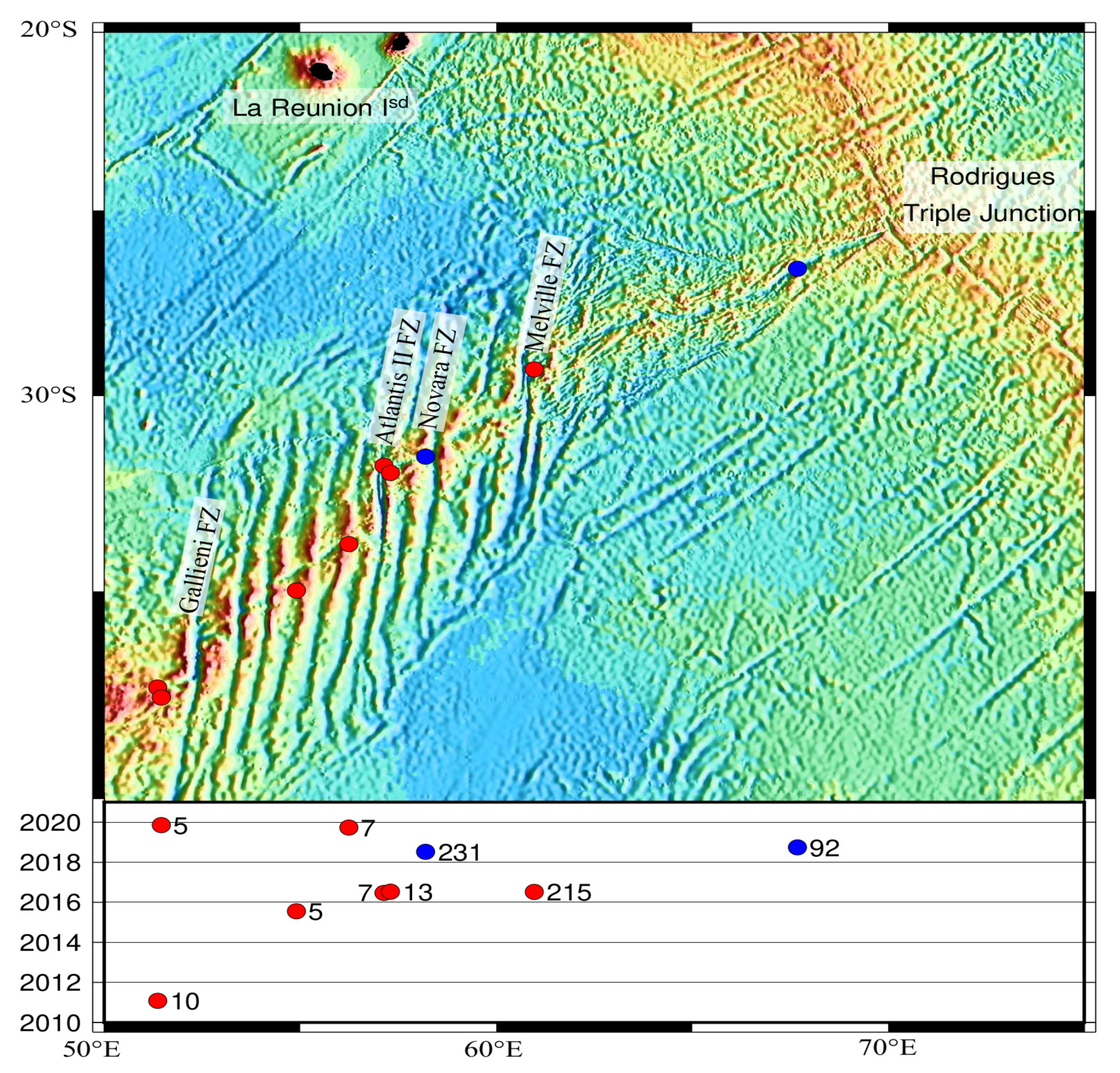
From 2010 to 2020, in the International Seismological Centre catalogue [45], we found only nine seismic swarms between 50° E and 70° E. We considered as swarms, the occurrence of at least five consecutive events within 15 days clustered in a grid of 3 × 3 degrees. Figure 1 shows their distribution: eight of them occurred west of Melville FZ and only one east of it. Most of them count about 10 or less (teleseismic) events, except three swarms: one in 2016 with 215 events and two in 2018 with 231 and 92 events. The latter two are remarkable: the one west of Melville FZ included the most Mw > 5 events (7) compared to the 2016 swarm (5); the one east of Melville FZ was the only one occurring in the nearly 1000 km long continuous section of the SWIR and also included 6 MW > 5 events. Their occurrence only a few months apart in two distinct tectonic settings made a further investigation worthwhile.
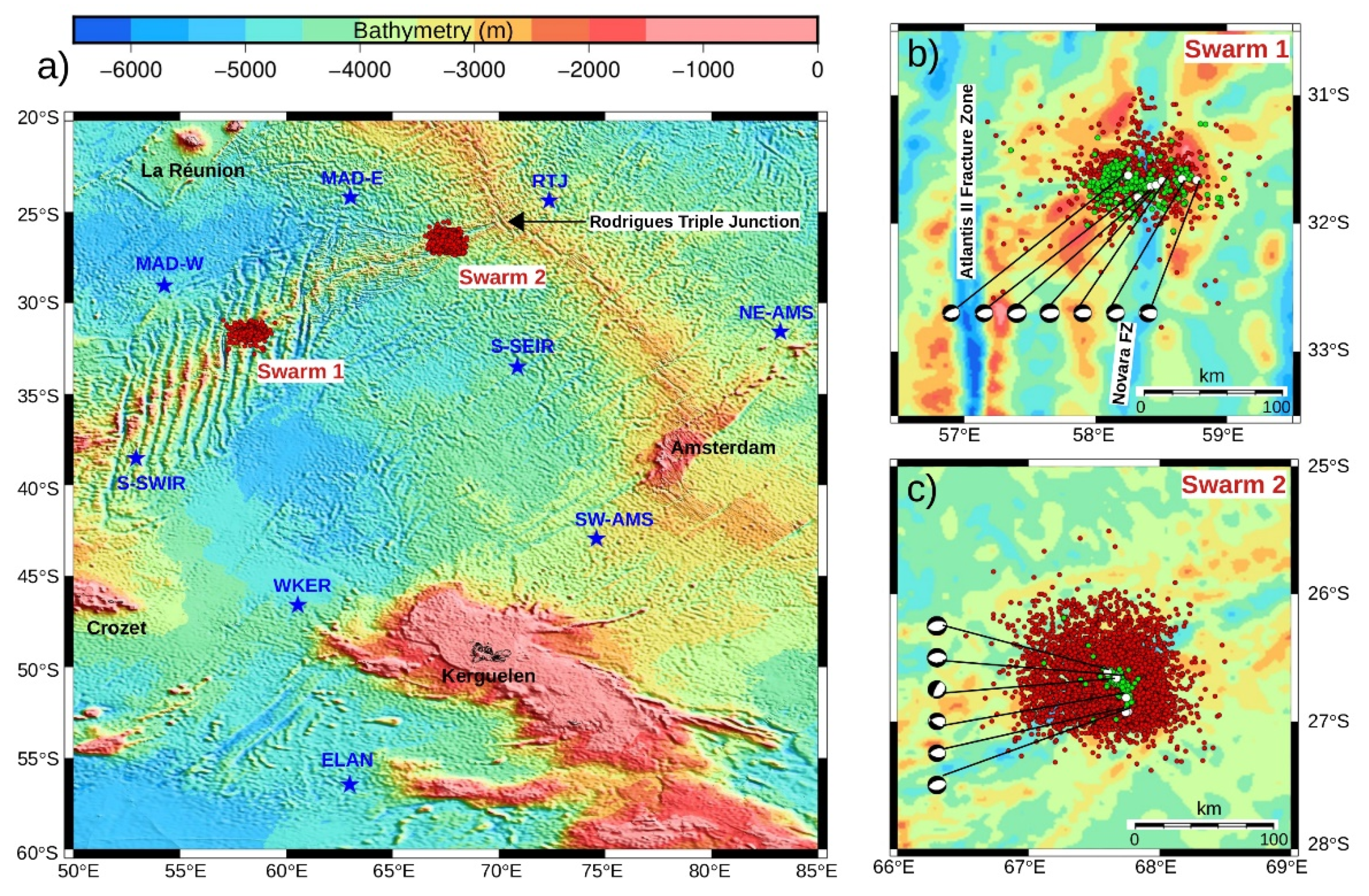
Based on the ISC catalogue, the first swarm (swarm-1) lasted for 6 days, from 10 July to 15 July 2018 and the second swarm (swarm-2) lasted for 31 days from 27 September to 27 October 2018 (Figure 2). Although locational uncertainties of the ISC catalogue are large (~20 km) in this remote part of the ocean, the occurrence of dense teleseismic events in a limited time period can be representative of seismic swarms [7]. Swarm-1 was located along SWIR Segment 18 at 58°10′ E (as numbered after Cannat et al. [35]) near the spreading-ridge intersection with the Novara FZ and comprised 231 events (Figure 2b). It started with a MW = 4.9 event on 10 July at 03h55. Seven events with a MW > 5.0 occurred after this onset and their focal mechanisms express normal faulting with azimuths parallel to the ridge axis. Swarm-2 occurred near a small axial discontinuity along SWIR Segment 4 at 67°40′ E, 220 km away from the RTJ and comprising 92 events (Figure 2c), started with a MW = 4.2 event on 27 September at 13h58. Six events with MW > 5.0 occurred afterward, also with normal faulting focal mechanisms approximately parallel to the ridge axis. The ISC catalogue events are more scattered in swarm-1 than in swarm-2.
To detect low-magnitude earthquakes associated with swarm-1 and swarm-2, lacking from land-based catalogues (due to the fact of their detection threshold) and to better understand whether these two swarms are tectonic or magmatic in origin, we examined hydroacoustic data (marine acoustic waves; T-waves) recorded by autonomous hydrophones (AuHs) moored on either side of the SWIR from the OHASISBIO network [47]. The OHASISBIO (Hydroacoustic Observatory of the Sismicity and Biodiversity in the Indian Ocean) is a long-term hydroacoustic program for monitoring the seismic activity and the vocal activity of large marine mammals in the southern Indian Ocean (e.g., [38,48]). The network is maintained during the yearly voyages of RV Marion Dufresne to the French Southern Islands. Since both swarms are located inside the OHASISBIO network, the observed hydroacoustic events have a more accurate location than the events from ISC catalogue. As the AuHs are also more sensitive to low-magnitude events, we detected 1109 hydroacoustic events for swarm-1 and 4880 events for swarm-2. There were thus five times more hydroacoustic events than the ISC catalogue for swarm-1 and 53 times more events for swarm-2. The analysis of this improved and dense catalogue of hydroacoustic events helps to understand the nature of these two swarms and the spreading processes that govern the SWIR.
2. Data and Methods
Because of the coherent nature of the propagation of sound waves in the ocean and the permanence of a well-defined oceanic sound–speed channel, hydrophone arrays provide a significant improvement in the detection threshold [49,50] and location accuracy [10,51,52] of earthquake events, relative to distant land-based seismic networks (as in the ISC catalogue). In this study, we analyzed data from an array of 9 hydrophones of the OHASISBIO network (Figure 2) that are moored in the SOFAR channel axis at depths ranging from 1000 m to 1300 m (Table 1). The hydrophones are located at the south of La Réunion Island (MAD-W and MAD-E), north-east and south-west of Amsterdam Islands (NE-AMS and SW-AMS), off the Southeast and Southwest Indian Ridges (S-SEIR and S-SWIR), near RTJ, west (WKER), and south-west (ELAN) of Kerguelen Island. They are set to record acoustic waves continuously at a rate of 240 Hz on 3 byte long samples. Their high-precision clocks are synchronized with a GPS clock before deployment and after recovery. The data from these hydrophones are analyzed with software developed at the Pacific Marine Environment Laboratory (PMEL) [10] and processed as described in Royer et al. [17].
To locate each earthquake, we picked the highest energy arrivals in the T-wave spectrograms [53,54]. After the identification of T-waves on three or more hydrophones, the source localization and origin time estimation were carried out by a non-linear least squares minimization of the arrival times on each of the hydrophones [10]. The errors in the latitude, longitude, and origin time were estimated from the covariance matrix of this least squares minimization, as modified by the mean square of the residuals. The distances and arrival times on each hydrophone were calculated using sound velocities in the ocean based on the Global Digital Environment Model (GDEM) and averaged along great circles joining the sources to each of the receivers [55]. It must be noted that the location of acoustic events actually corresponds to the location of the seismo-acoustic conversion on the seafloor. For shallow earthquakes, such as in a young oceanic crust, this point generally matches with the epicenter. However, in an area with high reliefs or near a seamount, the acoustic “radiator” may not exactly coincide with the epicenter [56]. In addition, T-waves do not provide any information about the depth of seismic events.
Acoustic events can be characterized by the acoustic magnitude or source level (SL) of the T-waves. The SLs are derived from the received levels at each hydrophone, corrected from the transmission loss between the event and the hydrophone locations. The received level (RL), expressed in decibels with respect to 1 micro-Pascal (dB re μPa at 1 m, hereinafter simply noted dB), corresponds to the maximum peak-to-peak amplitude in a 10 s time window centered on the peak of energy in the acoustic signal, in the 3–110 Hz frequency range, which closely resembles the definition of seismic amplitudes. The transmission loss (TL) comes from: (1) the cylindrical sound-spreading between the event location and the hydrophone; (2) the spherical sound-spreading in the water column between the sea-bottom acoustic radiator and the sound channel axis.
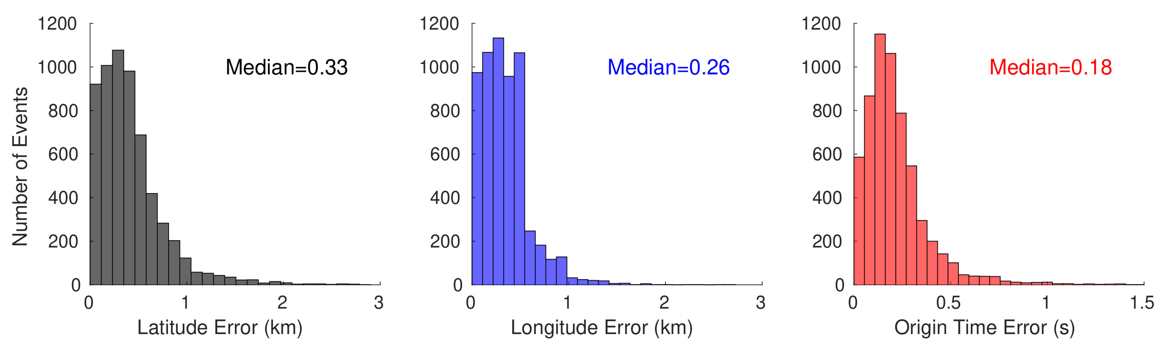
The analysis of the data was iterated twice for each swarm. We constructed a first hydroacoustic catalogue (OHA catalogue) containing event information such as the event ID; its latitude, longitude, and SL; the number and names of hydrophones used to locate the event; the calculated errors in the latitude, longitude, origin time, and SL. In a second iteration, we used this event information to re-pick and re-locate the hydroacoustic events. This step improved the catalogue by reducing the errors in latitude, longitude, and origin time by ~10-fold. The median errors in latitude, longitude, and origin time for all events from swarm-1 and swarm-2 (total 5989 events) were 0.33 km, 0.26 km, and 0.18 s, respectively (Figure 3). In the first iteration, the median errors were 4.33 km in latitude, 3.60 km in longitude, and 1.99 s in origin time; then, in the second iteration, the errors improved (by ~10-fold) to 0.44 km, 0.35 km, and 0.19 s, respectively, for swarm-1 events (Figure S1). Similarly, for swarm-2, the median errors improved (by ~11-fold) from 4.00 km to 0.33 km in latitude, 2.89 km to 0.26 in longitude, and 1.92 s to 0.18 in origin time (Figure S2).
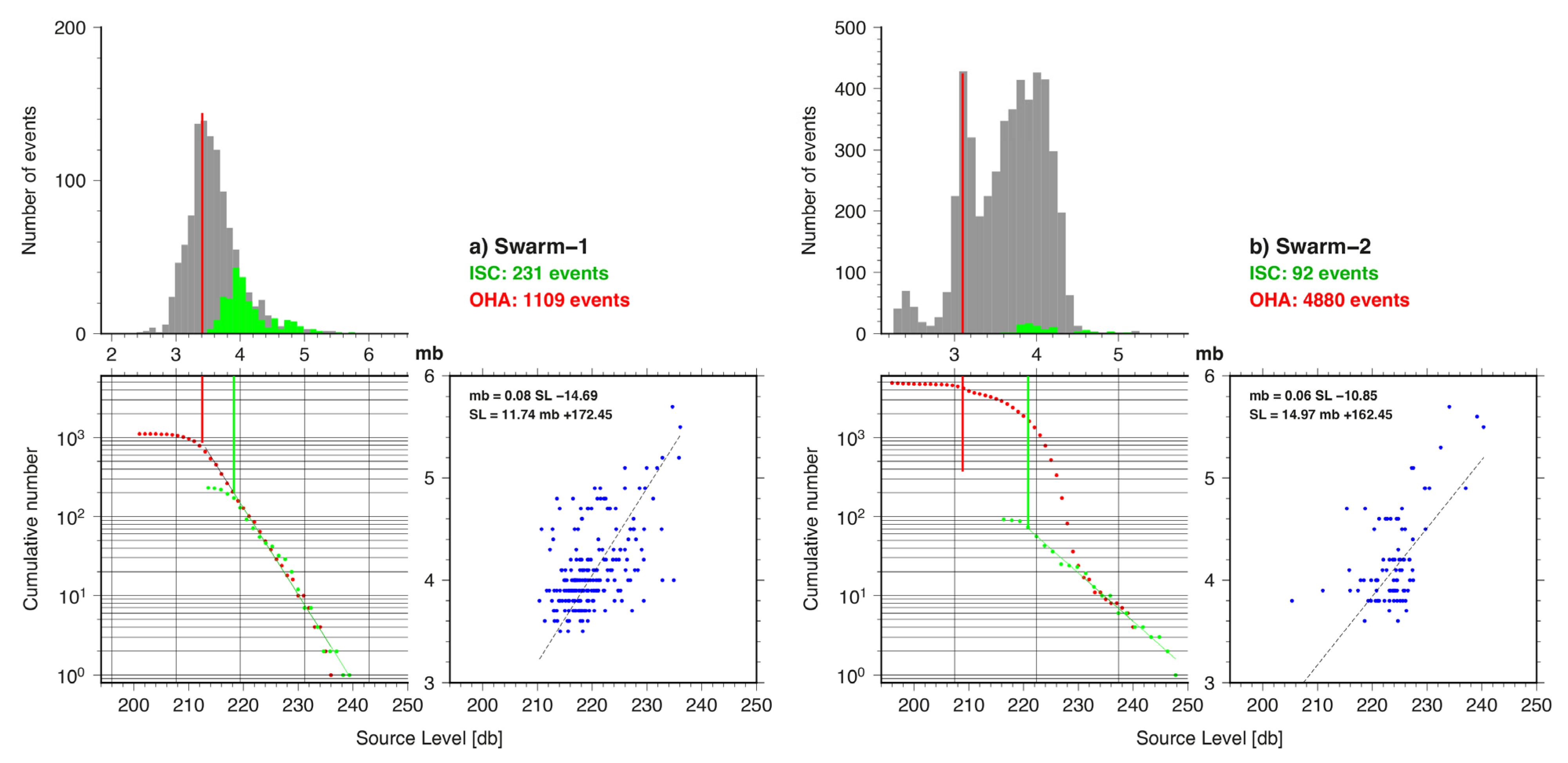
The detection threshold of an AuH array is defined by the SL of completeness (SLC) which is derived from the frequency–size distribution of the acoustic events [57]. It can be compared to the magnitude completeness of seismic events from land-based catalogues. Both are calculated by fitting a power–law relationship to the catalogue of events [58]:
where N is the cumulative number of events with a source-level greater or equal to SL, a and b are constants determined with the maximum likelihood method [59].
log(N) = a − b SL
For swarm-1, the ISC catalogue yielded a b-value of 2.96 (Figure 4a), much greater than the expected value of 1 typical for seismically active regions. The magnitude (mb) and SL of completeness of the ISC catalogue events were MC(ISC) = 3.9 mb and SLC(ISC) = 218 dB, respectively. For the OHA catalogue, the SLC was 6 dB lower and reached 212 dB, equivalent to MC(OHA) = 3.4 mb. This improvement in the magnitude of completeness led to ~5 times more events in the OHA catalogue than in the ISC catalogue (1109 vs. 231).
For swarm-2, the ISC catalogue yielded a b-value of 2.11 (Figure 4b), with a MC(ISC) = 3.9 mb and an SLC(ISC) = 220 dB, which are quite similar to swarm-1. However, the distribution of the SLs was very different, as they ranged from 207 to 225 dB and was bimodal with a sharp peak at 209 dB and a broad one centered on 220 dB (Figure 4b). Furthermore, swarm-2 had ~53 times more acoustic events than the ISC events (4880 vs. 92), with, among them, an unusually high number of low magnitude events yielding to an SLC(OHA) on the order of 209 dB. As a result, the cumulative log(N) curve was not straight and clearly departed from a characteristic power–law distribution for an SL < 231 dB. Comparing the completeness of the AuH records for both swarms was therefore not meaningful. Regardless, the improvement in the magnitude of the completeness of the OHA catalogue over the ISC catalogue demonstrated that hydrophone arrays provide more complete information about the seismicity along distant mid-oceanic ridges over land-based catalogues.
3. Results
3.1. Seismicity of Swarm-1
The iterative analysis of hydroacoustic records from the nine available AuHs starting from 6 July to 18 July 2018, yielded a total of 1137 events. This number was reduced to 1112 after selecting events with origin time-errors less than 10 s. We also excluded three events occurring at less than 40 s from the preceding event. Out of the remaining 1109 events (compared to 231 events in the ISC catalogue), 26 events (2%) were located with four hydrophones, 241 events (22%) with five AuHs, 445 events (40%) with six AuHs, 242 events (22%) with seven AuHs, 125 events (11%) with eight AuHs, and 30 events (3%) with nine AuHs. Only 325 events are discernible in the S-SWIR hydrophone records because of the high seasonal noise, and only 571 events in the ELAN hydrophone due to the fact of its long distance from the swarm (~2000 km).
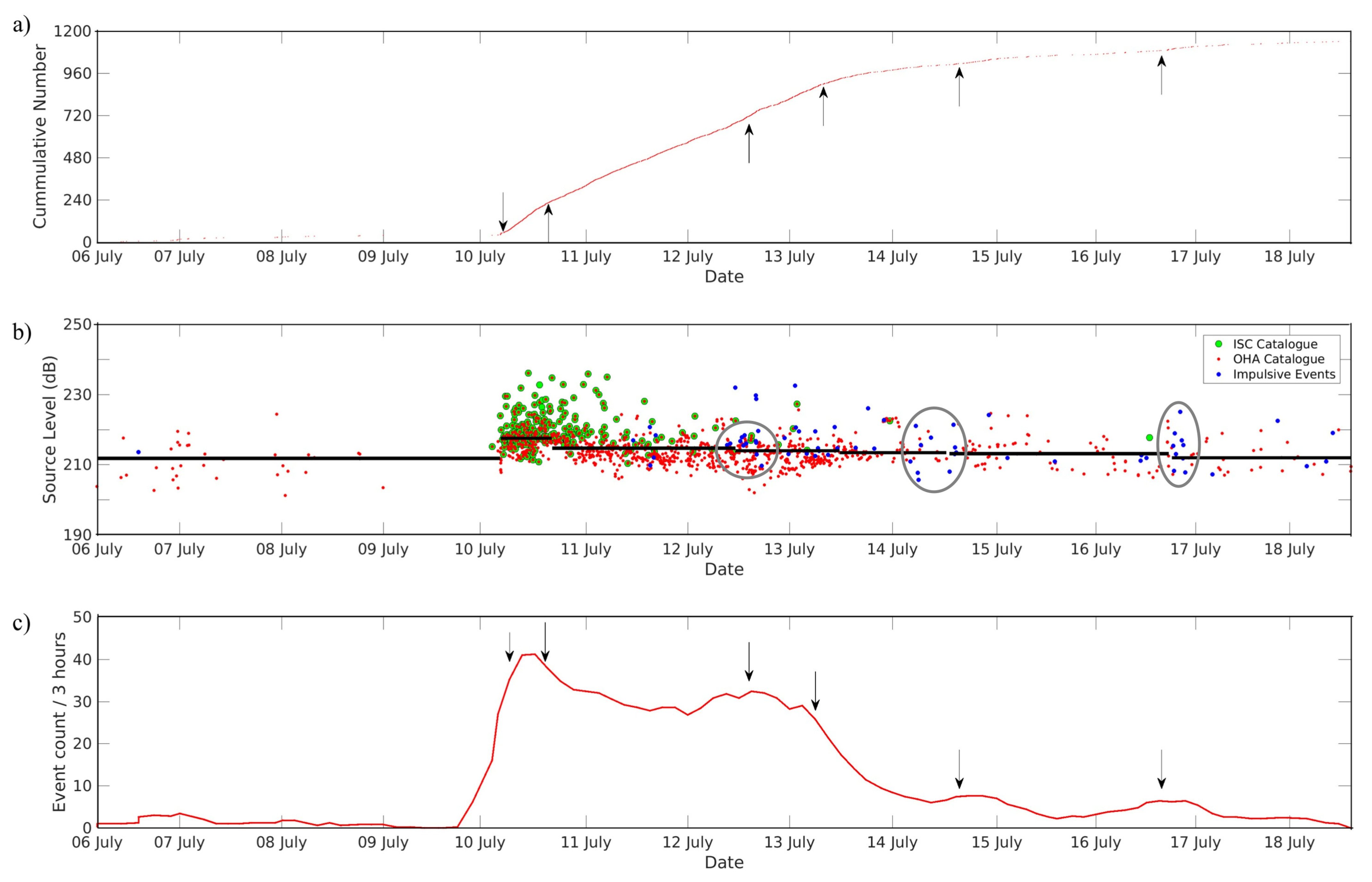
Between 6 July at 04h54 and the first strong event (10 July at 03h55, MW = 4.9), we found a total of 41 hydroacoustic events (Figure 5), representing very mild seismic activity. Starting 10 July at 03h55, 265 events occurred on 10 July and contributed to a sharp increase in the cumulative number (CN) of the events. Local changes in the seismic activity of the swarm are marked by black arrows in Figure 5a; they correspond to the times when there were local (short-term) changes in the event count (either an increase or a decrease) as seen in Figure 5c. At the swarm onset, the seismicity rose up to ~13 events per hour till 10 July at 16h00, after which it continued at a steady rate of ~10 events per hour for two days (Figure 5c). Between 10 July and the end of 12 July, the CN slope averaged ~250 events per day. Then, after 13 July, the seismic activity began to decline. The CN slope again changed on 14 July and 16 July due to the slight increase in the number of events. After 16 July, the CN curve was nearly flat until the last detected event of the swarm (18 July).
Changes in the CN slope on 12 July, 14 July, and 16 July coincided with the occurrence of a temporal cluster of impulsive events (blue dots/gray ellipses in Figure 5b). Those events were energetic and of short duration (<10 s) compared to the ~100 s duration of strong events (such as the events from the ISC catalogue; Figure 6). The short duration of the impulsive events may indicate that they were H-waves, meaning that the energy was released directly in the water and did not travel in the solid crust. Such impulsive events have previously been observed by Chadwick et al. [60] and Wilcock et al. [61,62] as associated with active and fresh lava flows at different underwater volcanoes. Clustered impulsive events have even been linked to isolated magma lenses [63]. Here, we detected 69 impulsive events. Three distinct temporal clusters of these impulsive events were observed: seven events on 12 July, 10 events on 14 July, and nine events on 16 July. These three temporal clusters coincided with noticeable changes in the CN slope; they resulted in a change in the seismic activity and an increase in the number of events for a short time (Figure 5c).
The SLs of the swarm-1 events ranged between 201.23 dB and 236.08 dB with a median of 212.20 dB. Ten events with an SL > 230 dB, thus highly energetic, were observed after the swarm onset (Figure 5b). These energetic events did not change the rate of seismic activity, and there was no dominating event with a higher SL. Out of these ten events, eight occurred on 10 and 11 July (green circles in Figure 5b) and the remaining two on 12 and 13 July (Table S1 in the Supplementary Materials). The median SL (SLM) of all 231 events from the ISC catalogue was 218.43 dB and 215.39 dB of all 69 impulsive events. The overall SL of the events before the swarm onset (6 July at 04h54 to 10 July at 03h51) was low with an SLM of 211.72 dB (thick black line in Figure 5b). The SL increased after the swarm onset, 10 July at 03h55, with the occurrence of abundant strong events, and remained near this level till 10 July at 16h00 with an SLM of 217.50 dB. After this, the SLs decreased together with the seismicity rate. After 10 July at 16h00, the SLM decreased to 214.66 dB till occurrence of the first cluster of impulsive events (12 July at 11h14) with SLM of 214.96 dB. Between 12 July at 11h14 and 13 July at 13h55 (time between the cluster of impulsive events and decreasing seismic activity), SLM of events reduces to 213.95 dB. From then on to the next cluster of impulsive events on 14 July at 12h55, the SLM decreased to 213.39 dB and then to 213.09 dB until 16 July at 17h17 (next two clusters of impulsive events), and finally down to 211.93 dB, till 18 July at 12h54 (end of the swarm). Though SLs do not directly represent seismic magnitudes, they follow the same pattern as the magnitude of events from the ISC catalogue, particularly at swarm onset.
3.2. Seismicity of Swarm-2
The swarm-2 analysis was based on hydroacoustic records from only seven AuHs (MAD-E and WKER AuHs recorded no data in the period of interest) and from 25 September to 27 October; this analysis led to the location of 5099 events. This number decreased to 5031 after selecting events with origin time-errors less than 10 s. We then removed all events within 40 s of the preceding one, yielding a catalogue of 4954 events (compared with 92 events in the ISC catalogue). After re-picking this first catalogue, 4880 events were relocated of which 782 events (16%) were located using four hydrophones, 2997 events (61.5%) using five, 1039 events (21%) using six, and 62 events (1.5%) using seven hydrophones. Only 2999 events were discernible in the S-SWIR records because of the high seasonal noise in the data and only 2039 events in ELAN data due to the fact of its remoteness from the swarm (~2500 km).
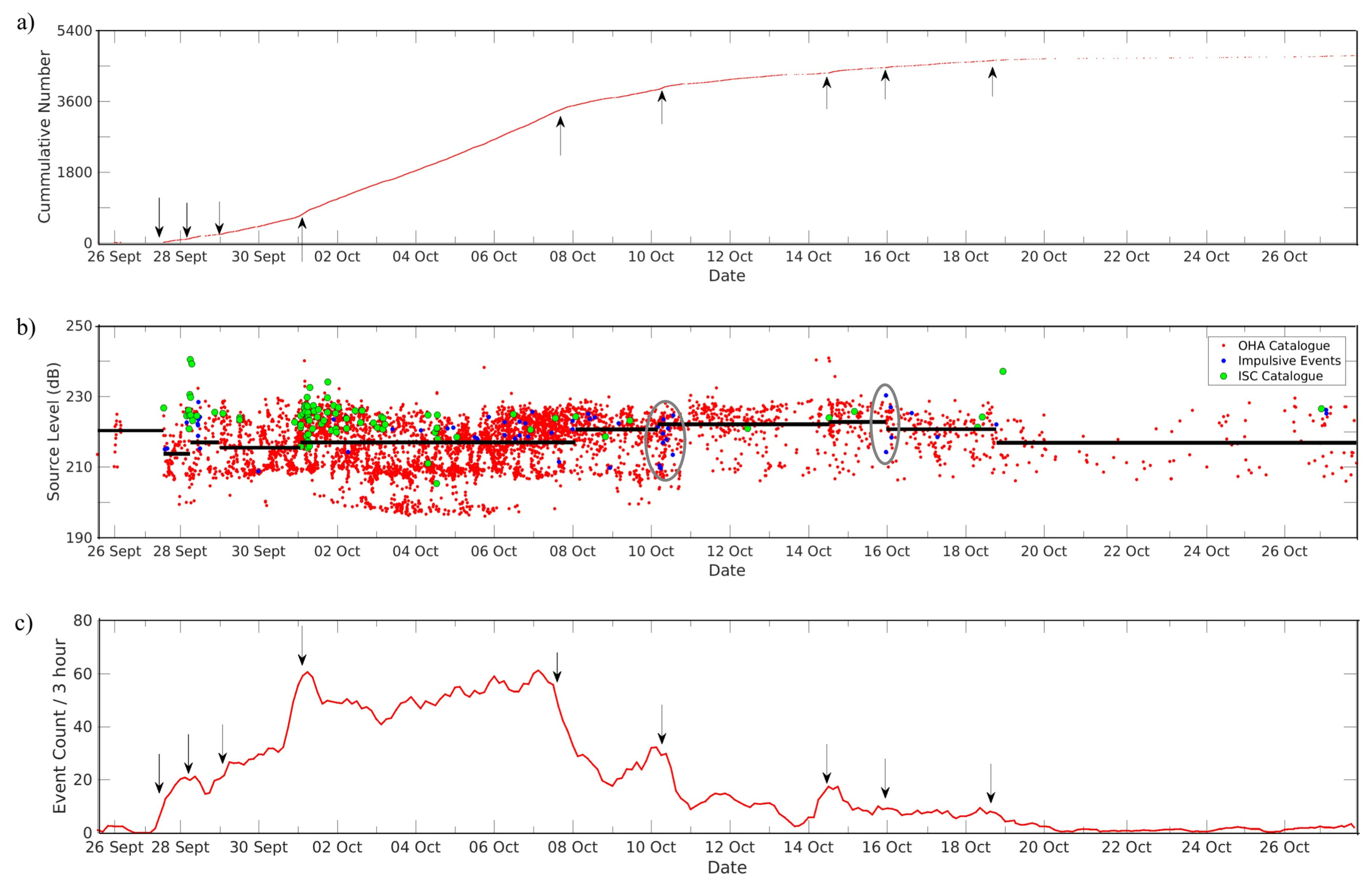
Only 17 events were detected between 25 September at 21h42 and 27 September at 13h58 (Figure 7), after which the seismicity slightly increased with one impulsive event and several small events, representing mild seismic activity. Similar to Figure 5, black arrows mark the time of changes in the CN slope (either an increase or a decrease in event count per unit of time). Starting from 28 September at 06h21, the swarm abruptly became active with the occurrence of a cluster of ten impulsive events (Figure 7a), leading to a sharp increase in the CN slope. The slope rose up again on 29 September. Seismicity became even more intense with 448 events on 1 October, among which the ISC catalogue lists a short duration temporal cluster. This intense seismic activity continued till 7 October with an average of ~414 events per day. During this period, the number of events increased per day, meaning the seismic activity intensified over time (Figure 7c). The CN slope slightly flattened at the start of 8 October, reflecting an abrupt decrease in seismic activity. The slope rose again on 10 October, with a cluster of ten impulsive events followed by short-time episodes of impulsive events. On 14 October, three strong events (SL > 230 dB) marked an increase in the event count (Figure 7c) with a cluster of five impulsive events at the end of 15 October. This activity declined after 18 October (SL > 230 dB) and remained even until the last detected event for this swarm (27 October).
In swarm-2, SLs ranged between 196.08 dB and 240.33 dB with a median of 217.70 dB (5.5 dB higher than for swarm-1), with 24 SLs > 230 dB (Figure 7b). Out of these 24 events, only seven are reported in the ISC catalogue (Table S2 in Supplementary Materials). The SLM of the 92 events in the ISC catalogue is 221.12 dB (2.69 dB higher than for swarm-1) and 221.16 for all 58 impulsive events (5.64 dB higher than that of swarm-1). Before the swarm onset, the SLM was 220.19 dB (25 September at 21h42 to 27 September at 13h58). It then decreased to 213.75 dB between the swarm onset and abrupt activation of the swarm (27 September at 13h58 to 28 September at 06h21), and at the end of 28 September, the SLM increased to 216.91 dB. Between 29 September and before the seismicity became intense (1 October at 01h36), the SLM decreased to 215.44 dB. During the period of intense seismic activity (1 to 7 October), the SLM increased to 216.94 dB and then to 220.63 dB during 8 to 10 October (before the occurrence of a cluster of impulsive events). It then attained the value of 222.09 dB till 14 October at 12h46 (matching a change in the CN slope) and then 222.69 dB till 15 October at 23h51 (occurrence of another cluster of impulsive events).
Before the occurrence of a strong event on 18 October at 22h53 (SL = 237.07 dB), the SLM decreased to 220.66 dB. In the end, the SLM decreased to 216.82 dB, as most of the detected events become sparser (constant slope in CN). Here, also, the SL of hydroacoustic events followed the same pattern as the magnitude of events in the ISC catalogue. The results relative to swarm-1 and -2 are summarized in Table 2.
In the case of swarm-1, we observed that the seismic activity (i.e., changes in CN slope) was governed by the occurrence of clusters of impulsive events. Whereas in swarm-2, the seismic activity changed after strong events, with the SL > 230 dB (e.g., on 28 September and 14 and 18 October). We interpreted the normal fault event on 28 September at 7 h 6 min (MW = 5.6 or SL = 239.4 dB at 26°55′ S, 67°44′ E) as a mainshock, because it was followed by 30 events over the next ~3.5 h within a distance of ~100 km (Figure S3), of which 22 were closely spaced in the vicinity of the mainshock (<40 km). Although these potential aftershocks had lower SLs, they did not follow a modified Omori law [64]. Similarly, the event on 14 October at 12h32 (SL = 240.79 dB; not reported in the ISC catalogue) was followed by 51 events within the next ~4.5 h and in a ~90 km radius (Figure S4). Here, also, subsequent events had lower SLs than the initial event, but did not follow a modified Omori law. Hence, these two sequences were not classical mainshock–aftershock sequences. The strong event on 18 October at 22h53 was also not followed by a pronounced increase in the seismic activity after its occurrence (i.e., the CN slope remains constant after). So, irrespective of the presence of relatively higher magnitude (or SL) events in swarm-2, there was no long exponential decay over several days in the aftershocks as in typical tectonic mainshock–aftershock sequences.
4. Discussion
4.1. Seismic Activity Rate
As expected from the large difference in the number of events and in their duration, the two swarms had very different seismic activity rates. Before the onset of swarm-1 (before 10 July at 03h55), there was only ~1 event per 2.5 h. After the swarm initiation, there were ~11 events per hour (E/H) for the first three days (10 to 12 July), then ~7 E/H between 12 and 14 July. It decreased to ~2 E/H from 14 to 16 July and then to just ~1 E/H till the end of the swarm. For swarm-2, there were ~1 E/H before the swarm onset. Then, ~6 and ~10 E/H from 27 to 28 September and from 29 September to 1 October, respectively. During the period of intense swarm activity (1 to 7 October), the rate increased to ~17 E/H, after which it progressively decreased to ~7 E/H between 8 and 10 October, to ~4 E/H between 10 and 16 October, to ~3 E/H till 18 October and down to ~1 event per 2 h from 18 October until the end of the swarm.
If we assume a uniform temporal distribution of events, the seismic activity rates were ~4 and ~8 E/H for swarm-1 and swarm-2 which span over 13 and 33 days, respectively; this shows that SWIR Segment 4 near the RTJ was seismically far more active than Segment 18 near the Novara FZ. This is indicative of different spreading processes likely due to the different thermal structures between a short ridge segment bounded by a high FZ wall and steep ridge flanks and a long continuous ridge segment. The latter, Segment 4, established ~10 Ma ago, as the result of the continuous eastward propagation of the SWIR, whereas the former, Segment 18, bounded by two large-offset fracture zones (Atlantis II and Novara FZs), is a long-lived spreading segment since ~55 Ma [27,28]. In comparison to the western part of the SWIR, the ridge section between the Melville FZ and the RTJ has no significant fracture zone offsets, transform or major discontinuities, and the axial valley is nearly continuous. Its depth is up to 2 km deeper than expected from Parsons and Sclater’s [65] plate cooling model. Seamount abundance is also lower than west of the Melville FZ [31]. Mantle S-wave velocities are higher [66]. These observations indicate that the subaxial crust and mantle temperatures are lower near Segment 4 than they are west of the Melville FZ, i.e., near Segment 18. This results in lower partial melting, less magma supply to the ridge axis, and thinner crust near Segment 4 [35]. This cooler mantle beneath Segment 4 will result in a higher lithospheric strength and thicker brittle layer more prone to accommodating numerous earthquake events. Indeed, large and low magnitude events are both clustered in a small area at Segment 18; in Segment 4, large magnitude events are clustered as well in the axial area, but the low magnitude events are spread over a wider area. The off-axis lithosphere of Segment 18 might therefore be less prone to tectonic seismicity than that of Segment 4 [18].
4.2. Temporal and Geographical Distribution of Events
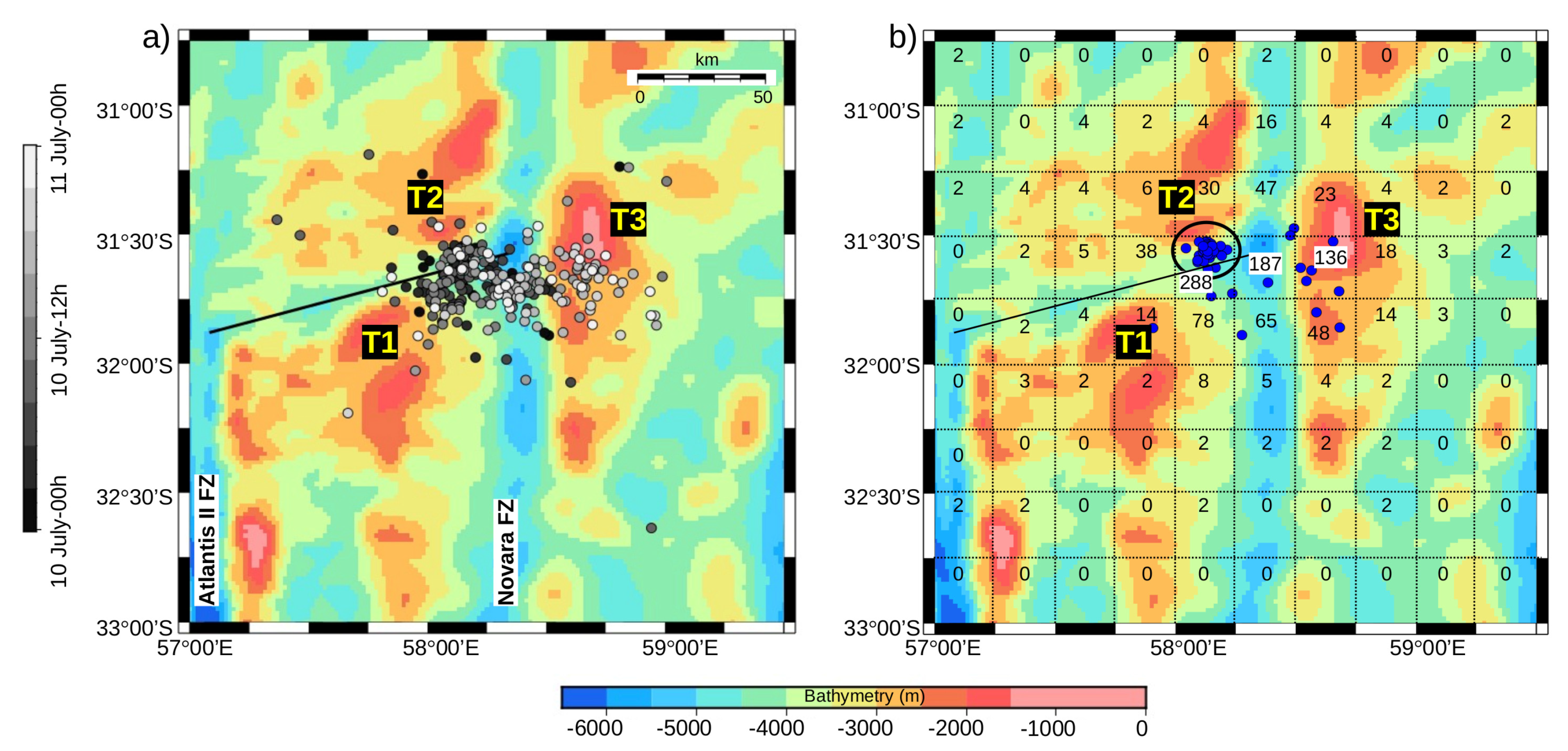
The swarm-1 events are mostly clustered between three seamounts: T1 at 32°00′ S, 58°00′ E (south seamount), T2 at 31°20′ S, 58°10′ E (north seamount), and T3 at 31°30′ S, 58°45′ E (high FZ crest to the East; Figure 8a and Figure S5a). Just after the onset of swarm-1 on 10 July, events seem to propagate in the east direction (Figure 8a and Figure S6). Before 10 July at 12 h, statistically, most of the events were located in the region between T1 and T2 (flanks of the N–S axial valley at 58°15′ E), and then between 10 July and 11 July at 00h, they occurred next to T3 (ridge-transform intersection). After 11 July at 00h, their distribution became random until the end of the swarm (lacking any spatial pattern; Figure S6). Gridding the number of hydroacoustic events every 1/4th degree in both latitude and longitude (dashed line grid in Figure 8b) shows that 55% of them were located between T1, T2, and T3 (highlighted in white), and were more numerous in the axial valley than in the transform valley. Also, most of the impulsive events clustered on the southern wall of the T2 seamount (the wall facing the axial valley at 31°35′ S, 58°12′ E). The decreasing number of events across the valley (west to east), the clustering of events between the three bathymetric highs, the initial eastward propagation pattern of events, and the absence of a relatively stronger event initiating the swarm suggest a magmatic origin. The swarm would have initiated with the propagation of several dikes from a same source which connect the seamounts, followed by the readjustment of stresses in the surrounding crust [50,67,68]. The stress readjustment rapidly fades away from the dike locus. The occurrence of three temporal clusters of impulsive events on 12 July, 14 July and 16 July on the southern wall of T2 (31°35′ S, 58°12′ E), followed by a minor increase in the event count (Figure 5c and Figure 8b) may represent the initiation and propagation of dikes from a source near T2. The T2 bathymetric high was more active compared to T1 and could represent an active volcanic center. The ridge T3, located across the transform, was located on an, at least, 10 Ma old oceanic crust and thus a priori inactive; however, the high and steep wall bounding of this elevated ridge constitutes an ideal radiator for T-waves. The apparent acoustic seismicity surrounding the summit of T3 is thus likely due to the fact of this artefact.
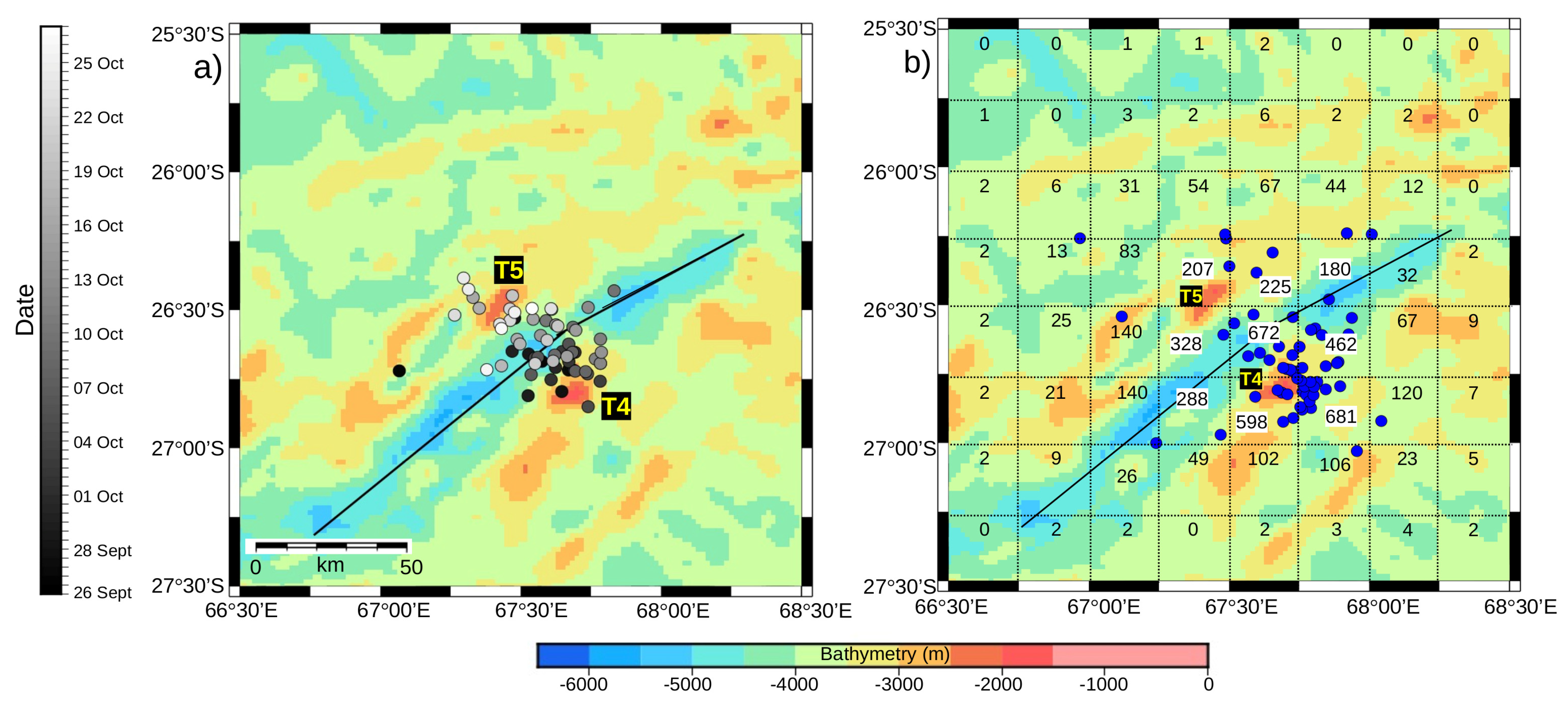
In the case of swarm-2, the events appeared to cluster between two bathymetric highs, T4 and T5, respectively at 26°52′ S, 67°38′ E, and 26°29′ S, 67°21′ E (T5 is NW of T4; Figure 9a and Figure S5b). The mean location of hydroacoustic events per 12 h from 26 September at 00h00 to 27 October at 12h00 (Figure 9a) was primarily concentrated near T4 before 20 October and then concentrated near T5 till the end of the swarm. It also spreads along the NE–SW bathymetric low separating T4 and T5. The spatio-temporal distribution of these averaged locations suggests an episodic cross-feeding of magma between T4 and T5 by a potential dike propagation [7,37]. It was also observed that the impulsive events were spatially located in the region surrounding T4 and T5 (Figure 9b). They were more clustered near T4 than T5 and, hence, T4 could represent the potential source of magma extrusion or dike initiation (volcanic center). The number of hydroacoustic events per 1/4th degree squares (dashed grid in Figure 9b) shows that 75% of the events were located near T4 and T5 (highlighted in white), a majority of events (2413 out of 4880) near T4, which again shows that it was more active. The decreasing number of events away from the two bathymetric highs supports the idea of a stress readjustment in the surrounding crust [50]. Moreover, the location of events reported in the ISC catalogue tends to align along a line joining these two seamounts (Figure 2c). This observation together with the focused impulsive events and the event temporal distribution also point for a magmatic origin for swarm-2, initiating with dike propagation from a source near T4.
If we compare the number and time distribution of events in swarm-1 and swarm-2, T4 was far more active than T2. Abundant numbers of impulsive events around T2 and T4 also suggest that fresh lava flows were exposed directly on the seafloor at the ridge crest. T2 and T4 seamounts were considered as isolated and shallow volcanic centers. The T2 volcanic center was in an area bounded with long-lived discontinuities (ridge–transform intersection), while T4 was in a region with relatively smoother topography, which would explain the wider spread of events in swarm-2 compared with that in swarm-1. The long distance and 4-month delay between these two swarms is representative of the behavior of a ultra-slow spreading ridge with episodic, distant, and focused magmatic supplies [33,69]. The spatio-temporal distribution of events in both swarms, together with the presence of volcanic centers, suggests a diking episode accompanied with magma movement, similar to that observed in Segment 7 [7,44].
4.3. Source Level of Earthquake Events
Although the geometrical spread of the ISC catalogue events was larger for swarm-1 than for swarm-2, that of the OHA catalogue events was smaller for swarm-1 (Figure 2). This observation might be explained by the fact that Segment 18 (locus of swarm-1) was already intensively fractured and might therefore be less prone to small-scale readjustment to local stress perturbation than Segment 4 (locus of swarm-2). The absence of weak (SL < 200 dB) events in the region of swarm-1 and their abundant number in swarm-2 (142 in total) indicates that Segment 4 is more brittle and, thus, more prone to stress readjustment after a local perturbation caused by strong events. The strong (SL > 230 dB) events are also more abundant (24 in total) in swarm-2 than swarm-1 (10 in total), suggesting that Segment 4 is more prone to tectonic fracturing than segment 18 [43]. After the onset of swarm-1, the progressive decrease of SLM (Figure 5b) reflects weaker stress readjustments over time until they stopped after 11 July. In swarm-2, the SLM of events first increased till 16 October after its strong activation on 28 September and then progressively decreased until no event became detectable. This gradual decrease in activity was interspersed with few strong events (Figure 7), which may represent renewed tectonic fracturing or dike intrusions, followed by further stress readjustments. After 16 October, the number of event detections drastically decreased, marking to termination of swarm-2.
4.4. Magmatic Nature of the Swarms
In swarm-1, during its apex from 10 July to 13 July, source levels were fairly homogeneous as the count of event per hour (Figure 5b,c), with no obvious mainshock–aftershock tectonic sequences. In swarm-2, there are three above average events on 28 September at 07h06, 14 October at 12h32, and 18 October at 22h53. However, none of them showed subsequent series of lesser events exceeding few hours; in addition, the source level dropped relative to the initial event was smaller than expected in mainshock–aftershock sequences (e.g., [1,70]). The strong events in swarm-2 do not resemble that found in tectonic swarms on other segments of the SWIR [43] or on other mid-oceanic ridges (e.g., [4,57,71]). The initial propagation of seismicity may indicate a magmatic intrusion, as observed from OBS data in SWIR Segment 7 [44]. Both swarms may therefore be mainly of magmatic nature, which, however, does not preclude the occurrence of normal faulting events [70]. The distribution of events with MW > 5 (white circles in Figure 2b,c), across Segments 4 and 18, could then represent the pathway for magma transport from a volcanic source to the neighboring seamounts [42,72,73]. We observed that the seismicity rate fluctuates over the time for both the swarms and that the normal fault events in the GCMT catalogue occurred later than the swarm onsets. Their later triggering probably reflects the stress-load histories of Segments 4 and 18 [42,74,75]. The observed initiation of magmatic activity and the occurrence of few large magnitude normal faulting events are consistent with the volcanic spreading events along the ultra-slow spreading Gakkel ridge [5,40,42]. The overall analysis of both the swarms suggest that they are both magmatic in origin, possibly triggered by dike intrusions and followed by stress readjustments in their vicinity as observed in Segment 7 [44]. The difference in duration, number, and SL range of events between the two swarms would reflect different lithospheric strength and stress load related to their different tectonic setting and heritage.
5. Conclusions
Due to the remoteness of the Southwest Indian Ridge, most of its seismicity is known from teleseismic records over several decades but limited to magnitudes larger than mb = 4.5. In situ seismicity recordings with ocean bottom seismometers are rare and limited in time (e.g., [7,41]). Long-term seismic monitoring with autonomous hydrophone networks bridges this gap by capturing lower magnitude (down to mb = 3.2) and transient events. Here, we analyzed the hydroacoustic activity associated with two swarms that occurred in 2018 along the SWIR, using data from the OHASISBIO hydrophone array. These two swarms occurred in contrasting tectonic contexts: swarm-1 on SWIR Segment 18, bounded by two large offset transform faults (Atlantis II and Novara FZ), swarm-2 on SWIR Segment 4, at a ridge discontinuity 200 km from the Rodrigues Triple Junction. The main findings of this study are:
- Swarm-1 lasted for 13 days and counted 1109 events and occurred at a long-lived ridge segment of the SWIR, whereas swarm-2 lasted for 33 days, counted 4880 events, and occurred at a younger ridge segment that resulted from the eastward propagation of the SWIR.
- The detection of events over two iterations reduced the uncertainties in location (latitude and longitude) and origin time by ∼10-fold in swarm-1 and ∼11-fold in swarm-2. For both swarms, they were better than 1 km in latitude and longitude and 0.5 s in origin time.
- In both swarms, we detected series of short duration (<10 s) impulsive events. Most of them focused on the slope of a local bathymetric high. We interpreted them as thermal explosions resulting from direct magma supply on the seafloor. The origin of dike intrusions may be located at their apex.
- Several observations, common to both swarms, pointed to a magmatic origin. The large events, detected on land (ISC; Mw > 5), and all hydroacoustic events occurred in an area bounded by or in the vicinity of bathymetric highs. Both showed an initial propagation, followed by spatio-temporal clusters and widespread stress readjustments. Finally, the absence of clear tectonic mainshock–aftershock sequences and a high seismicity rate are common signatures of a magmatic episode, and they lasted nearly two weeks in Segment 18 (swarm-1) and a month in Segment 4 (swarm-2).
- The abundance of weak (SL < 200 dB) and strong (SL > 230 dB) events in Segment 4 (locus of swarm-2) suggests that this end of the SWIR is more prone to small-scale readjustments to stress perturbations, here, dike intrusions, and to tectonic fracturing than long-lived, fracture zone bounded sections of the SWIR, such as Segment 18. The difference in the geometrical spread of small events, greater in swarm-2 than in swarm-1, is probably indicative of different lithospheric strengths.
Supplementary Materials
The following are available online at https://www.mdpi.com/article/10.3390/geosciences11060225/s1: Tables S1 and S2: Lists of the strongest acoustic events for both swarms (SL > 230 dB); Figures S1 and S2: Error distribution improvements in the picking iterations of the two swarms; Figures S3 and S4: Analysis of swarm-2 events after 28 September at 07h06 and 14 October at 12h32, 2018 events (respectively); Figure S5: Detailed bathymetric maps of the swarm areas: (a) For swarm-1; T1, T2 and T3 are three main local seamounts. (b) For swarm-2; T4 and T5 shows two local seamounts on either side of the rift valley; Figure S6: Distribution of swarm-1 events with respect to a reference point at west of it (showing an initial eastward propagation).
Author Contributions
Experiment conception and data acquisition, J.-Y.R.; Initial analysis, S.B. and J.-Y.R.; Formal analysis and original manuscript, V.V.I.; Manuscript review and edition, V.V.I., S.B. and J.-Y.R.; Resources, J.-Y.R. and S.B. All authors have read and agreed to the published version of the manuscript.
Funding
The French Polar Institute (IPEV) and the French Oceanographic Fleet funded the ship-time for the deployment and recovery cruises. INSU-CNRS provided additional support and the Regional Council of Brittany (CPER) funded the hydrophone moorings. V.V.I. was supported by a fellowship from the University of Brest and from the Regional Council of Brittany, through the ISblue project, Interdisciplinary Graduate School for the Blue Planet, co-funded by ANR (ANR-17-EURE-0015) and by the French government under the program “Investissements d’Avenir”.
Institutional Review Board Statement
Not applicable.
Informed Consent Statement
Not applicable.
Data Availability Statement
The data presented in this study are available on request from the corresponding author. The data will be publicly available through online repository after the publication.
Acknowledgments
The authors wish to thank the captains and crew of RV Marion Dufresne for the successful deployments and recoveries of the hydrophones of the OHASISBIO experiment. Figures were made with the Generic Mapping Tool (GMT; [76]). The authors acknowledge anonymous reviewers for their insightful comments and suggestions to improve the manuscript.
Conflicts of Interest
The authors declare no conflict of interest.
References
- Utsu, T. Aftershocks and earthquake statistics (2): Further investigation of aftershocks and other earthquake sequences based on a new classification of earthquake sequences. J. Fac. Sci. Hokkaido Univ. Ser. 7 Geophys. 1971, 3, 197–266. [Google Scholar]
- Passarelli, L.; Heryandoko, N.; Cesca, S.; Rivalta, E.; Rohadi, S.; Dahm, T.; Milkereit, C. Magmatic or not magmatic? The 2015–2016 seismic swarm at the long-dormant Jailolo volcano, West Halmahera, Indonesia. Front. Earth Sci. 2018, 6, 79. [Google Scholar] [CrossRef] [Green Version]
- Sykes, L.R. Earthquake swarms and sea-floor spreading. J. Geophys. Res. 1970, 75, 6598–6611. [Google Scholar] [CrossRef]
- Bergman, E.A.; Solomon, S.C. Earthquake swarms on the Mid-Atlantic Ridge: Products of magmatism or extensional tectonics? J. Geophys. Res. 1990, 95, 4943–4965. [Google Scholar] [CrossRef]
- Tolstoy, M.; Bohnenstiehl, D.R.; Edwards, M.H.; Kurras, G.J. Seismic character of volcanic activity at the ultraslow-spreading Gakkel Ridge. Geology 2001, 29, 1139–1142. [Google Scholar] [CrossRef]
- Schlindwein, V.; Demuth, A.; Korger, E.; Läderach, C.; Schmid, F. Seismicity of the Arctic mid-ocean ridge system. Polar Sci. 2015, 9, 146–157. [Google Scholar] [CrossRef]
- Schmid, F.; Schlindwein, V.; Koulakov, I.; Plötz, A.; Scholz, J.R. Magma plumbing system and seismicity of an active mid-ocean ridge volcano. Sci. Rep. 2017, 7, 42949. [Google Scholar] [CrossRef] [Green Version]
- Giusti, M.; Perrot, J.; Dziak, R.P.; Sukhovich, A.; Maia, M. The August 2010 earthquake swarm at North FAMOUS–FAMOUS segments, Mid-Atlantic Ridge: Geophysical evidence of dike intrusion. Geophys. J. Int. 2018, 215, 181–195. [Google Scholar] [CrossRef]
- Sykes, L.R. Mechanism of earthquakes and nature of faulting on the mid-oceanic ridges. J. Geophys. Res. 1967, 72, 2131–2153. [Google Scholar] [CrossRef] [Green Version]
- Fox, C.G.; Matsumoto, H.; Lau, T.K.A. Monitoring Pacific Ocean seismicity from an autonomous hydrophone array. J. Geophys. Res. 2001, 106, 4183–4206. [Google Scholar] [CrossRef]
- Korger, E.I.M.; Schlindwein, V. Performance of localization algorithms for teleseismic mid-ocean ridge earthquakes: The 1999 Gakkel Ridge earthquake swarm and its geological interpretation. Geophys. J. Int. 2012, 188, 613–625. [Google Scholar] [CrossRef] [Green Version]
- Toomey, D.R.; Solomon, S.C.; Purdy, G.M.; Murray, M.H. Microearthquakes beneath the median valley of the Mid-Atlantic Ridge near 23° N: Hypocenters and focal mechanisms. J. Geophys. Res. 1985, 90, 5443–5458. [Google Scholar] [CrossRef]
- Wolfe, C.J.; Purdy, G.M.; Toomey, D.R.; Solomon, S.C. Microearthquake characteristics and crustal velocity structure at 29° N on the Mid-Atlantic Ridge: The architecture of a slow spreading segment. J. Geophys. Res. 1995, 100, 24449–24472. [Google Scholar] [CrossRef]
- Tolstoy, M.; Waldhauser, F.; Bohnenstiehl, D.R.; Weekly, R.T.; Kim, W.-Y. Seismic identification of along-axis hydrothermal flow on the East Pacific Rise. Nature 2008, 451, 181–184. [Google Scholar] [CrossRef]
- Fox, C.G.; Radford, W.E.; Dziak, R.P.; Lau, T.K.; Matsumoto, H.; Schreiner, A.E. Acoustic detection of a seafloor spreading episode on the Juan de Fuca Ridge using military hydrophone arrays. Geophys. Res. Lett. 1995, 22, 131–134. [Google Scholar] [CrossRef]
- Smith, D.K.; Escartin, J.; Cannat, M.; Tolstoy, M.; Fox, C.G.; Bohnenstiehl, D.R.; Bazin, S. Spatial and temporal distribution of seismicity along the northern Mid-Atlantic Ridge (15°–35° N). J. Geophys. Res. 2003, 108, 2167. [Google Scholar] [CrossRef]
- Royer, J.Y.; Chateau, R.; Dziak, R.P.; Bohnenstiehl, D.R. Seafloor seismicity, Antarctic ice-sounds, cetacean vocalizations and long-term ambient sound in the Indian Ocean basin. Geophys. J. Int. 2015, 202, 748–762. [Google Scholar] [CrossRef] [Green Version]
- Rundquist, D.V.; Sobolev, P.O. Seismicity of mid-oceanic ridges and its geodynamic implications: A review. Earth Sci. Rev. 2002, 58, 143–161. [Google Scholar] [CrossRef]
- Bohnenstiehl, D.R.; Waldhauser, F.; Tolstoy, M. Frequency-magnitude distribution of microearthquakes beneath the 9°50′ N region of the East Pacific Rise, October 2003 through April 2004. Geochem. Geophys. Geosyst. 2008, 9, Q10T03. [Google Scholar] [CrossRef] [Green Version]
- Dziak, R.P.; Bohnenstiehl, D.R.; Smith, D.K. Hydroacoustic monitoring of oceanic spreading centers: Past, present, and future. Oceanography 2012, 25, 116–127. [Google Scholar] [CrossRef] [Green Version]
- Tolstoy, I.; Ewing, M. The T phase of shallow-focus earthquakes. Bull. Seism. Soc. Am. 1950, 40, 25–51. [Google Scholar] [CrossRef]
- Weston, D.E.; Rowlands, P.B. Guided acoustic waves in the ocean. Rep. Prog. Phys. 1979, 42, 347. [Google Scholar] [CrossRef]
- Fox, C.; Squire, V.A. On the oblique reflexion and transmission of ocean waves at shore fast sea ice. Phil. Trans. R. Soc. Lond. A 1994, 347, 185–218. [Google Scholar] [CrossRef]
- Royer, J.Y.; Patriat, P.; Bergh, H.W.; Scotese, C.R. Evolution of the Southwest Indian Ridge from the Late Cretaceous (anomaly 34) to the Middle Eocene (anomaly 20). Tectonophysics 1988, 155, 235–260. [Google Scholar] [CrossRef]
- Royer, J.Y.; Sclater, J.G.; Sandwell, D.T. A preliminary tectonic fabric chart of the Indian Ocean. Proc. Indian Acad. Sci. Earth Planet. Sci. 1989, 98, 7–24. [Google Scholar] [CrossRef] [Green Version]
- Sauter, D.; Cannat, M. The ultraslow spreading Southwest Indian ridge. In Diversity of Hydrothermal Systems on Slow Spreading Ocean Ridges; Geophysical Monograph Series; The American Geophysical Union: Washington, DC, USA, 2010; Volume 188, pp. 153–173. [Google Scholar] [CrossRef] [Green Version]
- Patriat, P.; Ségoufin, J. Reconstruction of the central Indian Ocean. Tectonophysics 1988, 155, 211–234. [Google Scholar] [CrossRef]
- Patriat, P.; Sauter, D.; Munschy, M.; Parson, L.M. A survey of the Southwest Indian Ridge axis between Atlantis II Fracture Zone and the Indian Triple Junction: Regional setting and large scale segmentation. Mar. Geophys. Res. 1997, 19, 457–480. [Google Scholar] [CrossRef]
- Chu, D.; Gordon, G.R. Evidence for motion between Nubia and Somalia along the Southwest Indian Ridge. Nature 1999, 398, 64–67. [Google Scholar] [CrossRef]
- Cannat, M.; Sauter, D.; Bezos, A.; Meyzen, C.; Humler, E.; Le Rigoleur, M. Spreading rate, spreading obliquity, and melt supply at the ultraslow spreading Southwest Indian Ridge. Geochem. Geophys. Geosyst. 2008, 9, Q04002. [Google Scholar] [CrossRef]
- Mendel, V.; Sauter, D.; Parson, L.; Vanney, J.R. Segmentation and morphotectonic variations along a super slow-spreading center: The Southwest Indian Ridge (57°–70° E). Mar. Geophys. Res. 1997, 19, 505–533. [Google Scholar] [CrossRef]
- Mendel, V.; Sauter, D.; Rommevaux-Jestin, C.; Patriat, P.; Lefebvre, F.; Parson, L.M. Magmato-tectonic cyclicity at the ultra-slow spreading Southwest Indian Ridge: Evidence from variations of axial volcanic ridge morphology and abyssal hills pattern. Geochem. Geophys. Geosyst. 2003, 4, 9102. [Google Scholar] [CrossRef]
- Dick, H.J.; Lin, J.; Schouten, H. An ultraslow-spreading class of ocean ridge. Nature 2003, 426, 405–412. [Google Scholar] [CrossRef] [PubMed]
- Sandwell, D.T.; Smith, W.H. Marine gravity anomaly from Geosat and ERS 1 satellite altimetry. J. Geophys. Res. 1997, 102, 10039–10054. [Google Scholar] [CrossRef] [Green Version]
- Cannat, M.; Rommevaux-Jestin, C.; Sauter, D.; Deplus, C.; Mendel, V. Formation of the axial relief at the very slow spreading Southwest Indian Ridge (49° to 69° E). J. Geophys. Res. 1999, 104, 22825–22843. [Google Scholar] [CrossRef]
- Wiens, D.A.; Petroy, D.E. The largest recorded earthquake swarm: Intraplate faulting near the Southwest Indian Ridge. J. Geophys. Res. 1990, 95, 4735–4750. [Google Scholar] [CrossRef]
- Krishna, M.R.; Arora, S.K. Space-time seismicity and earthquake swarms: Certain observations along the slow-spreading mid-Indian Ocean ridges. Proc. Indian Acad. Sci. Earth Planet. Sci. 1998, 107, 161–173. [Google Scholar] [CrossRef]
- Tsang-Hin-Sun, E.; Royer, J.Y.; Perrot, J. Seismicity and active accretion processes at the ultraslow-spreading Southwest and intermediate-spreading Southeast Indian ridges from hydroacoustic data. Geophys. J. Int. 2016, 206, 1232–1245. [Google Scholar] [CrossRef]
- Royer, J.Y.; Beauverger, M.; Torterotot, M.; Lecoulant, J. Seismic Crises along the Southwest Indian Ridge: Insights from Hydroacoustic Observations. 2019. Available online: https://agu.confex.com/agu/fm19/meetingapp.cgi/Paper/544476 (accessed on 20 May 2021).
- Schlindwein, V.; Schmid, F. Mid-ocean-ridge seismicity reveals extreme types of ocean lithosphere. Nature 2016, 535, 276–279. [Google Scholar] [CrossRef]
- Yu, Z.; Li, J.; Niu, X.; Rawlinson, N.; Ruan, A.; Wang, W.; Hu, H.; Wei, X.; Zhang, J.; Liang, Y. Lithospheric structure and tectonic processes constrained by microearthquake activity at the central ultraslow-spreading Southwest Indian Ridge (49.2° to 50.8° E). J. Geophys. Res. 2018, 123, 6247–6262. [Google Scholar] [CrossRef] [Green Version]
- Schlindwein, V. Teleseismic earthquake swarms at ultraslow spreading ridges: Indicator for dyke intrusions? Geophys. J. Int. 2012, 190, 442–456. [Google Scholar] [CrossRef] [Green Version]
- Läderach, C.; Korger, E.I.M.; Schlindwein, V.; Müller, C.; Eskstaller, A. Characteristics of tectonomagmatic earthquake swarms at the Southwest Indian Ridge between 16° E and 25° E. Geophys. J. Int. 2012, 190, 429–441. [Google Scholar] [CrossRef]
- Meier, M.; Schlindwein, V. First in situ seismic record of spreading events at the ultraslow spreading Southwest Indian Ridge. Geophys. Res. Lett. 2018, 45, 10–360. [Google Scholar] [CrossRef]
- ISC International Seismological Center. On-Line Bulletin 2021. Available online: http://www.isc.ac.uk/iscbulletin/search/catalogue/ (accessed on 10 November 2020).
- Ekström, G.; Nettles, M.; Dziewonski, A.M. The global CMT project 2004–2010: Centroid-moment tensors for 13,017 earthquakes. Phys. Earth Planet. Inter. 2012, 200–201, 1–9. [Google Scholar] [CrossRef]
- Royer, J.Y. OHA-SIS-BIO: Hydroacoustic Observatory of the Seismicity and Biodiversity in the Indian Ocean. 2009. Available online: https://campagnes.flotteoceanographique.fr (accessed on 21 May 2021).
- Samaran, F.; Stafford, K.M.; Branch, T.A.; Gedamke, J.; Royer, J.-Y.; Dziak, R.P.; Guinet, C. Seasonal and geographic variation of southern blue whale subspecies in the Indian Ocean. PLoS ONE 2013, 8, e71561. [Google Scholar] [CrossRef]
- Fox, C.G.; Dziak, R.P.; Matsumoto, H.; Schreiner, A.E. Potential for monitoring low-level seismicity on the Juan-de-Fuca ridge using military hydrophone arrays. Mar. Technol. Soc. J. 1993, 27, 22–30. [Google Scholar]
- Dziak, R.P.; Smith, D.K.; Bohnenstiehl, D.R.; Fox, C.G.; Desbruyeres, D.; Matsumoto, H.; Tolstoy, M.; Fornari, D.J. Evidence of a recent magma dike intrusion at the slow spreading Lucky Strike segment, Mid-Atlantic Ridge. J. Geophys. Res. 2004, 109, B12102. [Google Scholar] [CrossRef] [Green Version]
- Bohnenstiehl, D.R.; Tolstoy, M. Comparison of teleseismically and hydroacoustically derived earthquake locations along the north-central Mid-Atlantic Ridge and Equatorial East Pacific Rise. Seism. Res. Lett. 2003, 74, 791–802. [Google Scholar] [CrossRef]
- Bohnenstiehl, D.R.; Tolstoy, M.; Smith, D.K.; Fox, C.G.; Dziak, R.P. Time-clustering behavior of spreading-center seismicitybetween 15 and 35 N on the Mid-Atlantic Ridge: Observations from hydroacoustic monitoring. Phys. Earth Planet. Int. 2003, 138, 147–161. [Google Scholar] [CrossRef]
- Schreiner, A.E.; Fox, C.G.; Dziak, R.P. Spectra and magnitudes of T-waves from the 1993 earthquake swarm on the Juan de Fuca Ridge. Geophys. Res. Lett. 1995, 22, 139–142. [Google Scholar] [CrossRef]
- Slack, P.D.; Fox, C.G.; Dziak, R.P. P wave detection thresholds, Pn velocity estimates, and T wave location uncertainty from oceanic hydrophones. J. Geophys. Res. 1999, 104, 13061–13072. [Google Scholar] [CrossRef]
- Teague, W.J.; Carron, M.J.; Hogan, P.J. A comparison between the Generalized Digital Environmental Model and Levitus climatologies. J. Geophys. Res. 1990, 95, 7167–7183. [Google Scholar] [CrossRef]
- Lecoulant, J.; Guennou, C.; Guillon, L.; Royer, J.-Y. 3D-modeling of earthquake generated acoustic waves in the ocean in simplified configurations. J. Acoust. Soc. Am. 2019, 146, 2110–2120. [Google Scholar] [CrossRef]
- Bohnenstiehl, D.R.; Tolstoy, M.; Dziak, R.P.; Fox, C.G.; Smith, G. Aftershock sequences in the mid-ocean ridge environment: An analysis using hydroacoustic data. Tectonophysics 2002, 354, 49–70. [Google Scholar] [CrossRef]
- Gutenberg, B.; Richter, C.F. Seismicity of the Earth and Associated Phenomena; Princeton University Press: Princeton, NJ, USA, 1954. [Google Scholar]
- Aki, K. Maximum likelihood estimate of b in the formula log N = a−b M and its confidence limits. Bull. Earthq. Res. Inst. Tokyo Univ. 1965, 43, 237–239. [Google Scholar]
- Chadwick, W.W.; Paduan, J.B.; Clague, D.A.; Dreyer, B.M.; Merle, S.G.; Bobbitt, A.M.; Caress, D.W.; Philip, B.T.; Kelley, D.S.; Nooner, S.L. Voluminous eruption from a zoned magma body after an increase in supply rate at Axial Seamount. Geophys. Res. Lett. 2016, 43, 12063–12070. [Google Scholar] [CrossRef]
- Wilcock, W.S.; Tolstoy, M.; Garcia, C.; Tan, Y.J.; Waldhauser, F. Live from the Seafloor: Seismic Signals Associated with the 2015 Eruption of Axial Seamount. 2015. Available online: https://agu.confex.com/agu/fm15/meetingapp.cgi/Paper/73407 (accessed on 20 May 2021).
- Wilcock, W.S.; Tolstoy, M.; Waldhauser, F.; Garcia, C.; Tan, Y.J.; Bohnenstiehl, D.R.; Caplan-Auerbach, J.; Dziak, R.P.; Arnuif, A.F.; Mann, M.E. Seismic constraints on caldera dynamics from the 2015 Axial Seamount eruption. Science 2016, 354, 1395–1399. [Google Scholar] [CrossRef] [Green Version]
- Tan, Y.J.; Tolstoy, M.; Waldhauser, F.; Wilcock, W.S. Dynamics of a seafloor-spreading episode at the East Pacific Rise. Nature 2016, 540, 261–265. [Google Scholar] [CrossRef]
- Utsu, T.; Ogata, Y.; Matsuura, R.S. The centenary of the Omori formula for a decay law of aftershock activity. J. Phys. Earth 1995, 43, 1–33. [Google Scholar] [CrossRef]
- Parsons, B.; Sclater, J.G. An analysis of the variation of ocean floor bathymetry and heat flow with age. J. Geophys. Res. 1977, 82, 803–827. [Google Scholar] [CrossRef]
- Debayle, E.; Lévêque, J.-J. Upper mantle heterogeneities in the Indian Ocean from waveform inversion. Geophys. Res. Lett. 1997, 24, 245–248. [Google Scholar] [CrossRef]
- Sohn, R.A.; Hildebrand, J.A.; Webb, S.C. Postrifting seismicity and a model for the 1993 diking event on the CoAxial segment, Juan de Fuca Ridge. J. Geophys. Res. 1998, 103, 9867–9877. [Google Scholar] [CrossRef]
- Rivalta, E.; Taisne, B.; Bunger, A.P.; Katz, R.F. A review of mechanical models of dike propagation: Schools of thought, results and future directions. Tectonophysics 2015, 638, 1–42. [Google Scholar] [CrossRef] [Green Version]
- Michael, P.J.; Langmuir, C.H.; Dick, H.J.B.; Snow, J.E.; Goldstein, S.L.; Graham, D.W.; Lehnert, K.; Kurras, G.; Jokat, W.; Mühe, R.; et al. Magmatic and amagmatic seafloor generation at the ultraslow-spreading Gakkel ridge, Arctic Ocean. Nature 2003, 423, 956–961. [Google Scholar] [CrossRef]
- McNutt, S.R. Seismic monitoring and eruption forecasting of volcanoes: A review of the state-of-the-art and case histories. In Monitoring and Mitigation of Volcano Hazards; Springer: Berlin/Heidelberg, Germany, 1996; pp. 99–146. [Google Scholar] [CrossRef]
- Simao, N.; Escartin, J.; Goslin, J.; Haxel, J.; Cannat, M.; Dziak, R. Regional seismicity of the Mid-Atlantic Ridge: Observations from autonomous hydrophone arrays. Geophys. J. Int. 2010, 183, 1559–1578. [Google Scholar] [CrossRef] [Green Version]
- Cannat, M.; Rommevaux-Jestin, C.; Fujimoto, H. Melt supply variations to a magma-poor ultra-slow spreading ridge (Southwest Indian Ridge 61° to 69° E). Geochem. Geophys. Geosyst. 2003, 4, 9104. [Google Scholar] [CrossRef]
- Standish, J.J.; Sims, K.W. Young off-axis volcanism along the ultraslow-spreading Southwest Indian Ridge. Nat. Geosci. 2010, 3, 286–292. [Google Scholar] [CrossRef] [Green Version]
- Mogi, K. Earthquakes and fractures. Tectonophysics 1967, 5, 35–55. [Google Scholar] [CrossRef]
- Hainzl, S. Seismicity patterns of earthquake swarms due to fluid intrusion and stress triggering. Geophys. J. Int. 2004, 159, 1090–1096. [Google Scholar] [CrossRef]
- Wessel, P.; Smith, W.H. New, improved version of Generic Mapping Tools released. Eos Trans. Am. Geophys. Union 1998, 79, 579. [Google Scholar] [CrossRef]
Figure 1.
Bathymetric map of the Southwest Indian Ridge, between 50° E and 70° E, showing the geographic and temporal distribution of swarms reported in the ISC catalogue from 2010 to 2020. The numbers next to the symbols refer to the number of teleseismic events in the ISC catalogue for each individual swarm. The blue dots show the location of the two 2018 swarms investigated in this paper.

Figure 2.
The locations of the two 2018 swarms along the Southwest Indian Ridge: (a) hydroacoustic events (red dots) detected by the OHASISBIO network of hydrophones (blue stars); (b,c) enlarged sections for swarm-1 along ridge Segment 18 and swarm-2 along ridge Segment 4 with the hydroacoustic events (red dots), events from the land-based ISC catalogue (green dots), and events with MW > 5.0 (white dots) along with their focal mechanisms (GCMT catalogue [46]).

Figure 3.
Distribution of errors in the location (i.e., latitude and longitude) and origin time of all hydroacoustic events in swarm-1 and swarm-2 after two iterations of detection and localization.
Figure 3.
Distribution of errors in the location (i.e., latitude and longitude) and origin time of all hydroacoustic events in swarm-1 and swarm-2 after two iterations of detection and localization.

Figure 4.
Completeness of the acoustic catalog based on the source levels (SLs) and ISC magnitude (mb) of all events from (a) swarm-1 and (b) swarm-2. The correspondence between the SL and mb scales was based on matching the best-fitting Gutenberg–Richter lines up to the completeness values outlined in green for the ISC catalogue and in red for the OHA catalogue. The upper graph shows the histogram of the hydroacoustic events (gray) and the ISC catalogue events (green). The lower left graph shows the cumulative number of events in the OHA catalogue (red) and ISC catalogue (green). The vertical red and green line denotes the completeness values of the SLs and mb of the OHA and ISC catalogue, respectively. The lower right graph shows the SL-to-mb relationship (and reciprocal) and trend line, obtained from the cumulative number of events.

Figure 5.
Temporal distribution of Swarm-1 events: (a) Cumulative number (CN) of events vs. time since the origin of the time axis. Black arrows point to changes in the CN slope. (b) Source level distribution of all hydroacoustic events (red dot), impulsive events (blue dot), and events reported in the ISC catalogue (green circles). Thick black lines define the median SL (SLM) for events occurring between two consecutive black arrows in (a). The gray colored ellipses denote the cluster of impulsive events. (c) Number of events per 3 h in a moving window shifted by intervals of 30 min. The black arrows point to local changes in the event count.

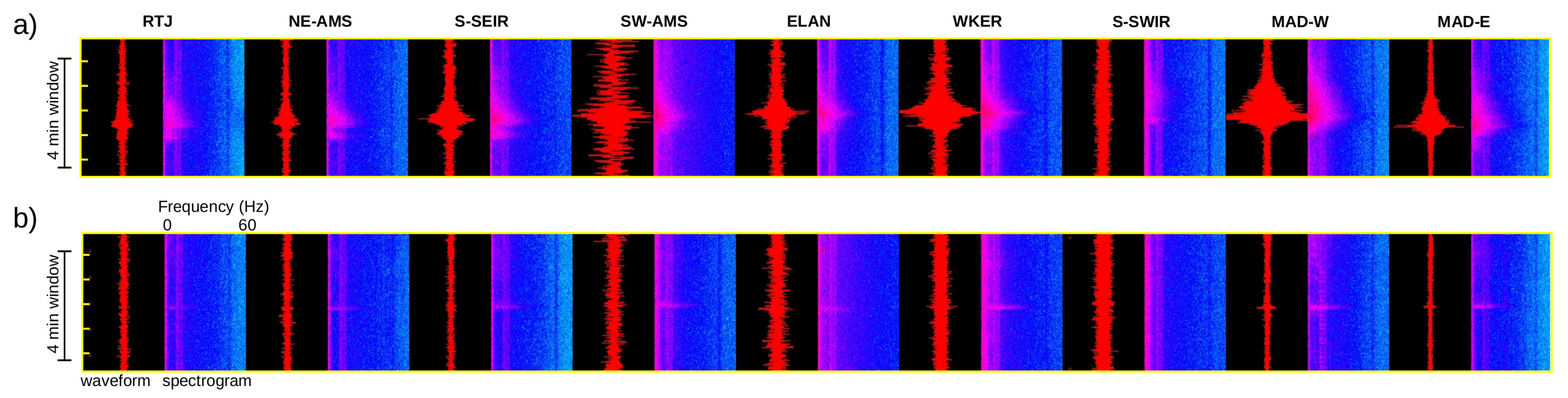
Figure 6.
Four-minute-long waveform and corresponding spectrogram of (a) a strong event on 10 July at 03h55 and (b) an impulsive event on 11 July at 16h11 on all nine hydrophones of the OHASISBIO network. The signal for strong event lasts for ~100 s vs. ~10 s for impulsive event. Due to the presence of seasonal noise in the S-SWIR records, the signal was weak for the strong event and absent for the impulsive event.

Figure 7.
Temporal distribution of Swarm-2 events: (a) cumulative number (CN) of events vs. time since the origin of the time axis. Black arrows point to changes in the CN slope; (b) source level distribution of all hydroacoustic events (red dot), impulsive events (blue dot), and events reported in the ISC catalogue (green circles). Thick black lines define the median SL (SLM) for events occurring between two consecutive black arrows in (a). The gray colored ellipses denote the cluster of impulsive events; (c) Number of events per 3 h in a moving window shifted by intervals of 30 min. Black arrows point to local changes in the event count.

Figure 8.
(a) Temporal distribution of location of events between 10 July at 00h and 11 July at 00h. T1, T2, and T3 are local bathymetric highs in the swarm-1 region. The black line shows the axial valley in Segment 18. The gray color scale denotes the origin time of events from 10 July at 00h to 11 July at 00h. (b) Location of all impulsive events (blue dots). Numbers in grid squares are the total event count in each ¼th grid of latitude and longitude for the entire swarm duration; the highest counts among the seamounts are highlighted in white.

Figure 9.
(a) Temporal distribution of mean location (as mean latitude and mean longitude) of swarm-2 events over the bin size of 12 h (gray color scale). T4 and T5 are local bathymetric highs in swarm-2 region. (b) Location of all impulsive events (blue dots). They were mostly clustered towards T4. Numbers in grid squares are the total event count in each ¼th grid of latitude and longitude for the entire swarm duration; the highest counts around T4 and T5 seamounts are highlighted in white. The black line shows the location of axial valley in Segment 4.


Table 1.
Locations and parameters of the autonomous hydrophones of the OHASISBIO network.
| Sites | RTJ | NE-AMS | S-SEIR | SW-AMS | ELAN | WKER | S-SWIR | MAD-W | MAD-E |
|---|---|---|---|---|---|---|---|---|---|
| Latitude (°S) | 24.379 | 31.576 | 33.518 | 42.951 | 56.460 | 46.602 | 38.547 | 29.047 | 24.205 |
| Longitude (°E) | 72.372 | 83.242 | 70.866 | 74.598 | 62.976 | 60.548 | 52.929 | 54.258 | 63.010 |
| Depth (m) | 1109 | 1060 | 1280 | 1100 | 1020 | 960 | 1230 | 1288 | 1238 |
| Sampling rate (Hz) | 240 | 240 | 240 | 240 | 240 | 240 | 240 | 240 | 240 |
| Sensitivity (dB) | −163.9 | −163.5 | −163.7 | −163.4 | −163.8 | −163.3 | −164.2 | −163.4 | −163.5 |
| Start time | 11 February 2018 | 5 February 2018 | 8 February 2018 | 31 January 2018 | 16 January 2018 | 19 January 2018 | 9 January 2018 | 6 January 2018 | 13 February 2018 |
| End time | 10 February 2019 | 30 January 2019 | 23 December 2018 | 30 January 2019 | 23 January 2019 | 29 July 2018 | 14 January 2019 | 3 November 2018 | 21 July 2018 |
| Clock drift (ppm) | 0.0300 | −0.2426 | −0.2861 | 0.0048 | −0.0222 | −0.0348 | 0.0346 | −0.0010 | −0.7870 |
Table 2.
Summary of the analyses of the hydroacoustic data from the OHASISBIO AuH network.
| Key Points | Swarm 1 | Swarm 2 |
|---|---|---|
| Date span in 2018 | 6 July to 18 July | 25 September to 27 October |
| Duration in days | 13 | 33 |
| Number of ISC catalogue events | 231 | 92 |
| Number of hydroacoustic events | 1109 | 4880 |
| Average number of events per hour (over whole duration) | 4 | 8 |
| Number of impulsive events | 69 | 58 |
| Number of AuH stations used | 9 | 7 |
| Most events located with | 6 stations (40%) | 5 stations (62%) |
| Median error in latitude (km) | 0.44 | 0.33 |
| Median error in longitude (km) | 0.35 | 0.26 |
| Median error in origin time (s) | 0.19 | 0.18 |
| Range of source level (dB) | 201.23–236.08 | 196.08–240.33 |
| Number of events with SL > 230 dB | 10 | 24 |
| Number of events with SL < 200 dB | 0 | 142 |
| SL of completeness of OHA catalogue | 212 dB | 209 dB |
| SL of completeness of ISC catalogue (Figure 4) | 218 dB | 223 dB |
| Magnitude completeness of ISC catalogue (mb) | 3.9 | 3.9 |
| Magnitude completeness of OHA catalogue (mb, Figure 4) | 3.4 | 3.1 |
Publisher’s Note: MDPI stays neutral with regard to jurisdictional claims in published maps and institutional affiliations. |
© 2021 by the authors. Licensee MDPI, Basel, Switzerland. This article is an open access article distributed under the terms and conditions of the Creative Commons Attribution (CC BY) license (https://creativecommons.org/licenses/by/4.0/).
Share and Cite
MDPI and ACS Style
Ingale, V.V.; Bazin, S.; Royer, J.-Y. Hydroacoustic Observations of Two Contrasted Seismic Swarms along the Southwest Indian Ridge in 2018. Geosciences 2021, 11, 225. https://doi.org/10.3390/geosciences11060225
AMA Style
Ingale VV, Bazin S, Royer J-Y. Hydroacoustic Observations of Two Contrasted Seismic Swarms along the Southwest Indian Ridge in 2018. Geosciences. 2021; 11(6):225. https://doi.org/10.3390/geosciences11060225
Chicago/Turabian StyleIngale, Vaibhav Vijay, Sara Bazin, and Jean-Yves Royer. 2021. "Hydroacoustic Observations of Two Contrasted Seismic Swarms along the Southwest Indian Ridge in 2018" Geosciences 11, no. 6: 225. https://doi.org/10.3390/geosciences11060225
Note that from the first issue of 2016, this journal uses article numbers instead of page numbers. See further details here.