Assessing the Reliability of Earthquake Environmental Effects in Historical Events: Insights from the Southern Apennines, Italy


1
Dipartimento di Scienza e Alta Tecnologia, Università degli Studi dell’Insubria, Via Valleggio 11, 22100 Como, Italy
2
Independent Consultant, Via della Resistenza 171, 00185 Cantalice (Rieti), Italy
3
Istituto Nazionale di Geofisica e Vulcanologia, Sezione Roma 1, Via di Vigna Murata 605, 00143 Roma, Italy
*
Author to whom correspondence should be addressed.
Geosciences 2020, 10(9), 332; https://doi.org/10.3390/geosciences10090332
Submission received: 28 July 2020
/
Revised: 20 August 2020
/
Accepted: 20 August 2020
/
Published: 22 August 2020
(This article belongs to the Special Issue Earthquake Environmental Effects in the Historical and Recent Data)
Abstract
:Earthquake Environmental Effects (EEEs) are a common occurrence following moderate to strong seismic events. EEEs are described in literary sources even for earthquakes that occurred hundreds of years ago, but their potential for hazard assessment is not fully exploited. Here we analyze five earthquakes occurred in the Southern Apennines (Italy) between 1688 and 1980, to assess if EEEs are reliable indicators of the effects caused by past earthquakes. We investigate the spatial distribution of EEEs and their ability to repeatedly occur at the same place, and we quantitatively compare the macroseismic fields expressed in terms of damage-based intensity (MCS: Mercalli–Cancani–Sieberg) to the Environmental Scale Intensity (ESI) macroseismic field, derived from an intensity attenuation relation. We computed the field “ESI-MCS”, showing that results are consistent when comparing different seismic events and that ESI values are higher in the first ca. 10 km from the epicenter, while at distances greater than 20 km MCS values are higher than ESI. Our research demonstrates that (i) EEEs offer a detailed picture of earthquake effects in the near field and (ii) the reappraisal of literary sources under a modern perspective may provide improved input parameters that are useful for seismic hazard assessment.

1. Introduction
A proper and comprehensive assessment of the seismic risk of a region should include both the characterization of potential seismogenic sources and the pattern of damage expected due to ground shaking. Macroseismology and historical seismology analyze available documentation of the effects of past earthquakes to gain information on the cause (i.e., the earthquake itself; [1]). The quantity and quality of available data obviously affects the resolution and reliability of the results: information on earthquakes that occurred decades to centuries ago is usually fragmentary or incomplete.
Traditionally, according to the Mercalli–Cancani–Sieberg (MCS), Modified Mercalli (MM) and Medvedev–Sponheur–Karnik (MSK) scales, the assignment of macroseismic intensity is based on the effects on humans, the natural environment and the built environment [1,2]. With the introduction of the European Macroseismic Scale (EMS), effects on the natural environment were explicitly neglected, because they considered unreliable and “of limited use” [3]. The EMS scale is therefore particularly suitable for assessing the damage to different building types; however, it significantly deviates from the original scales, hampering the comparison between different earthquakes, and especially historical ones. In 2007, the Environmental Seismic Intensity (ESI) scale was introduced; it is based exclusively on Earthquake Environmental Effects (EEEs; [4,5]). The ESI scale is complementary to damage-based scales and provides useful information, especially when traditional scales saturate (above an intensity of ca. IX) or cannot be applied (e.g., remote areas with sparse settlements).
In this paper, our aim is to demonstrate, through the analysis of five case histories in a homogeneous territorial setting, that EEEs repeat consistently in time and provide complementary information when compared to traditional, damage-based intensity scales. To reach this goal, here we analyze five earthquakes that occurred in the Southern Apennines (Italy) between 1688 and 1980, to assess if EEEs are reliable indicators of the effects caused by past seismic events, that occurred either in the pre-instrumental or instrumental era. We analyze the spatial distribution of EEEs and we quantitatively compare the MCS/MSK fields with an ESI theoretical field derived from a recently published attenuation relation [6].
In this paper we briefly present the local seismotectonic setting and seismicity and we describe the dataset and adopted methods, explaining how we derived the ESI macroseismic fields and how we compared them to MCS/MSK fields. Moreover, we analyze the obtained results: first, we analyze the spatial distribution of EEEs, with particular reference to the 1694, 1930 and 1980 earthquakes that hit the same region; then, we compute the ESI macroseismic field and the difference “ESI-MCS” and finally we discuss the results in the broader context of a historical reading of EEEs and their reliability as diagnostics for either historical or recent earthquakes.
2. Seismotectonic Setting and Seismicity
The Southern Apennines are a Neogene fold-and-thrust belt dominated by carbonate and clastic sequences and controlled by the subduction of the Adriatic plate to the East and the back-arc Tyrrhenian Sea to the West [7,8,9,10]. The main active faults are of extensional type and arranged in a narrow belt, which runs close to the axis of the Apennines chain. The characteristics of capable faults and seismogenic sources are summarized in the ITHACA (ITaly HAzard from CApable faults) and DISS (Database of Italian Seismogenetic Sources) databases [11,12]. The region hosts frequent seismicity, often characterized by seismic sequences (i.e., series of earthquakes with comparable magnitude; [13]), a focal depth ranging in the 5–20 km interval and a maximum magnitude of ca. Mw 7.0 [14,15]. Historical documentation and macroseismic studies are abundant [16].
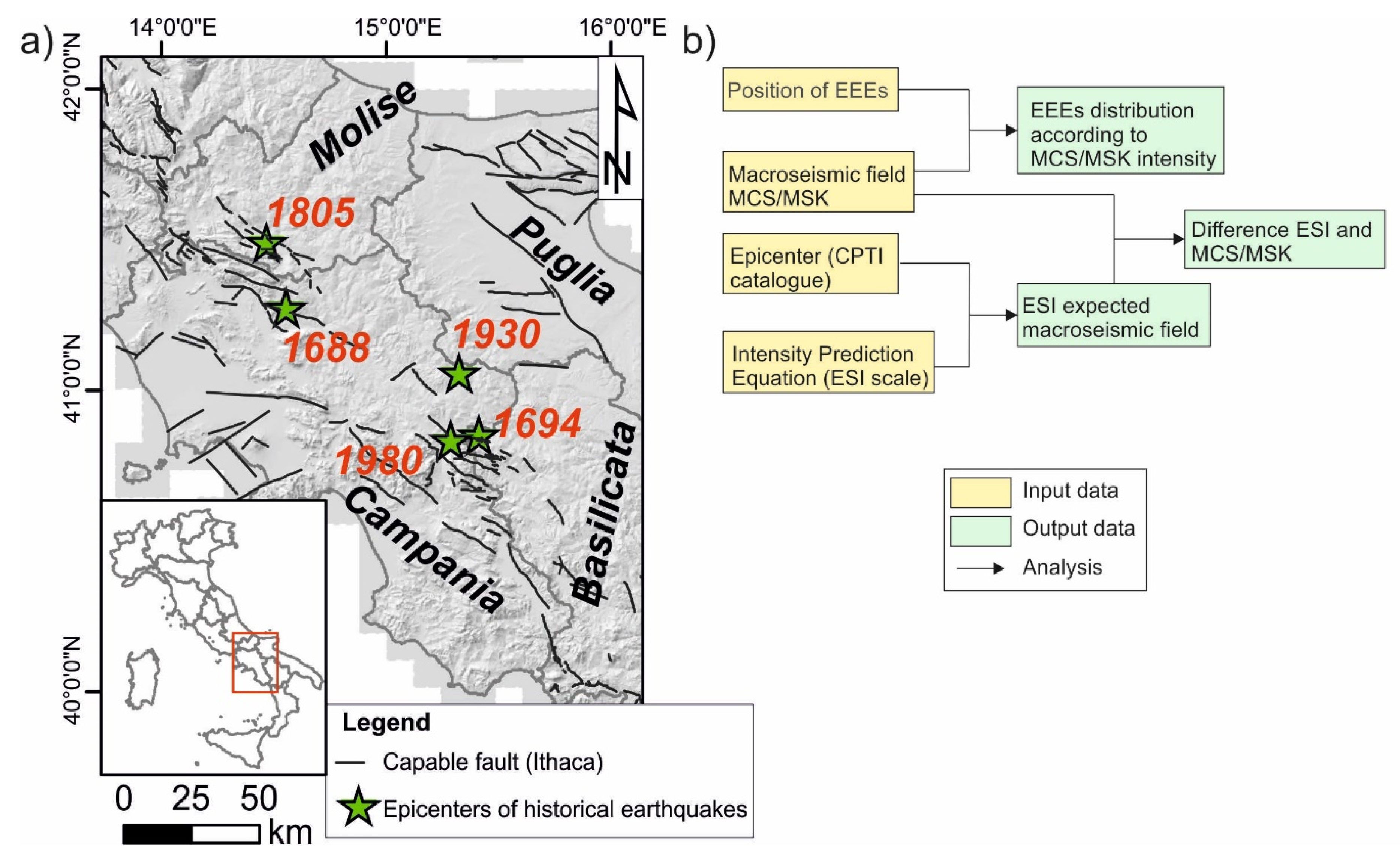
Here we analyze five seismic events that occurred between 1688 and 1980 (Figure 1a); they all had a normal-faulting mechanism and Mw between 6.7 and 7.1 [14]. The 1688 and 1805 earthquakes hit the Molise region and part of Campania, while the 1694, 1930 and 1980 ones mainly struck the area of the Campania, Basilicata and Puglia regions. The causative source of the 1805 Molise earthquake is considered a NE-dipping structure along the slopes of the Matese Massif and surface faulting with vertical displacement of up to 1.5 m were documented [11,17]. The source of the 1688 earthquake has not been unequivocally identified so far, although there are hypotheses put forward by some authors [18,19,20,21].
The 1980 earthquake showed a complex seismological pattern, with three sub-events that occurred within 40 seconds. The activated faults stroke NW–SE and surface faulting was documented at several sites [22,23,24]; general consensus exists about a NE dip direction of the first two shocks and a SW dip direction of the third shock [11]. The 1694 earthquake was considered a twin of the 1980 earthquake, but paleoseismological studies to date failed to identify surface faulting associated with the 1694 event [23]. The 1930 earthquake hit an area adjacent to the epicentral zone of the 1980 earthquake, but slightly to the NE; offsets of up to 40 cm were documented [16,25].
3. Materials and Methods
We gathered available data for each of the studied earthquakes, including epicentral coordinates [14], description and location of EEEs, and macroseismic fields expressed in terms of MCS or MSK intensity. EEEs were categorized in five classes according to the type of effect: surface faulting, slope movement, ground breaks, hydrological/hydrogeological anomalies and liquefaction. Table 1 lists the five earthquakes analyzed in this study; the epicentral intensity I0 on the MCS/MSK scale was X for all the events except for the 1688 (I0 XI). On the other hand, ESI epicentral intensity, assessed based on the surface rupture length or area affected by secondary effects, was X for all earthquakes [26].
The number of localities where EEEs were documented increased with time: about 15 data points were assigned to the two 17th century earthquakes, while over 100 localities were assessed for the 1980 earthquake. EEEs descriptions were compiled at the “site” level, that is, each place where an environmental effect was recorded; sites were then grouped into “localities” and an ESI intensity value was assigned to each locality [5]; here we analyzed the data generalized at the locality level.
An ESI macroseismic field was not available for all the earthquakes, so we derived it from an intensity prediction equation (IPE), which expresses the ESI intensity as a function of epicentral intensity I0 and distance. The equation was developed by the authors of [6] from over 400 ESI intensity data points belonging to 14 earthquakes that occurred in the Central and Southern Apennines; data were binned according to the intensity value, and the median value for each class was used to derive the prediction equation adopting a least-squares approach. A log-linear functional form was selected based on the fitting performance. The IPE assumed the following values [6]:
where I0 is the ESI epicentral intensity and R is the epicentral distance in km.
The IPE assumed an isotropic attenuation of intensity with distance; thus the derived isoseismals were circular. Macroseismic fields were generally elongated with a strike similar to the seismogenic source, but available data for the ESI scale were not considered sufficient to fully describe this spatial asymmetry; it must be recalled that the ESI scale was introduced ca. 15 years ago [4] and that the IPE proposed by the authors of [6] is the first attenuation equation for the ESI scale worldwide.
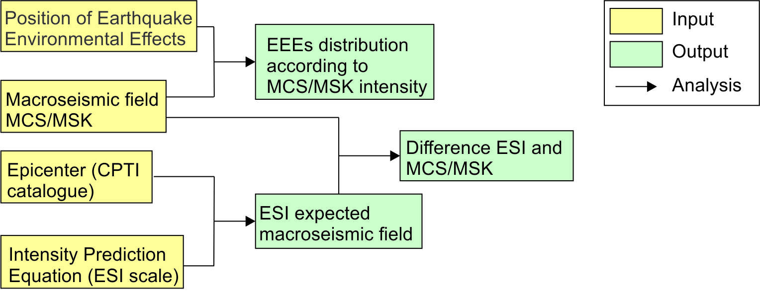
The methodological workflow of our research is presented in Figure 1b. In a first step, we analyzed the MCS/MSK intensity at each location where an EEE was documented; we focused on the 1694, 1930 and 1980 seismic events, because they hit the same region (Section 4.1). In a second step, we compared the MCS/MSK macroseismic fields with the ESI macroseismic field derived from Equation (1) (Section 4.2). Since all five earthquakes shared a common epicentral intensity (I0 ESI = X, see Table 1), we inverted the equation and derived the radii of ESI isoseismals for intensities between VI and X. Results are presented in Table 2. We drew the ESI isoseismals centered on the macroseismic epicenter and we computed the difference “ESI-MCS” on a grid of 1 km2 cells.
4. Results
On the basis of the data and analysis given in Section 3, we will now illustrate the results on EEEs distribution and the quantitative comparison of MCS/MSK and ESI macroseismic fields. We investigated the presence of systematic differences in the intensity pattern as derived from the damage to the built environment (MCS and MSK scales) or to the natural environment (ESI scale). Such variations were evaluated with respect to the distance from the epicenter and the direction of the seismogenic sources.
4.1. EEEs Distribution
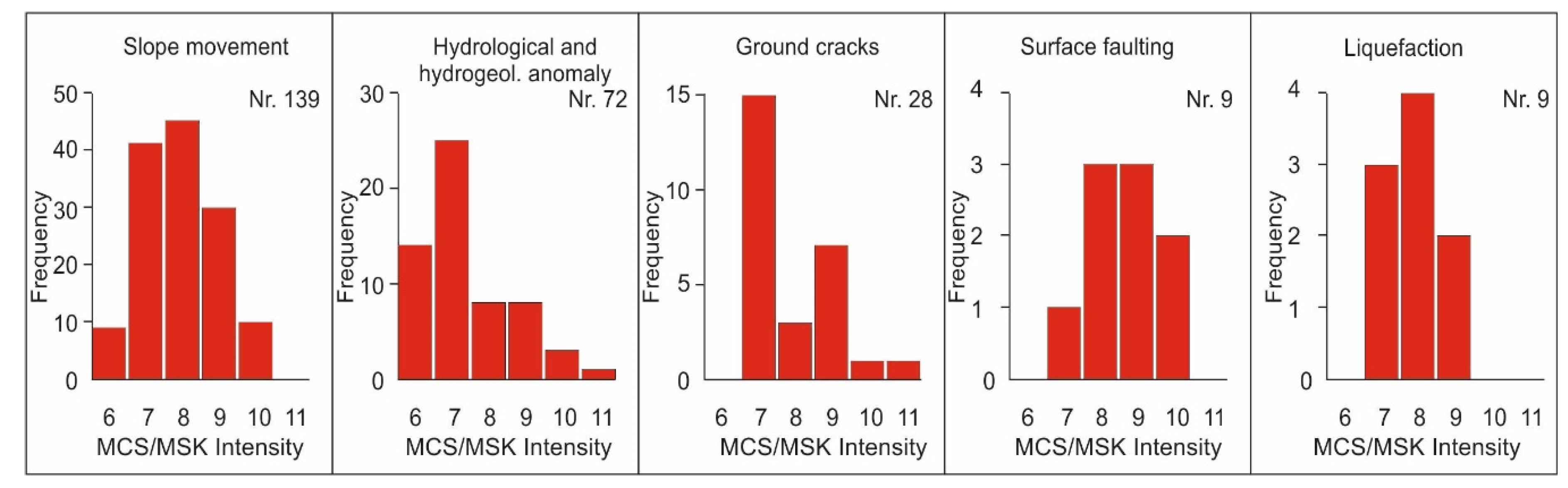
In this study we compared the distribution of EEEs for each class of MCS/MSK intensity for the five earthquakes. Figure 2 shows the distribution in frequency of the five categories of EEEs. EEEs were widespread for an intensity value I > VII, but each type had a distinct distribution: the most frequently documented effects were slope movements (139 occurrences), 62% of which occurred for intensity values of I = VII–VIII. Hydrological and hydrogeological anomalies were recorded mainly at values I = VI–VII (54%). These percentage values are not surprising data, since this type of effect is also common in the far field (for example, [17,29]). The cracks in the ground were widespread for an intensity value of I = VII (54%) while liquefaction was an effect that occurred for intensity values of I = VII–IX.
Primary effects (i.e., surface faulting) were documented at only nine localities, 89% of which had an intensity value of I ≥ VIII. This higher threshold was expected because on-fault effects occur by definition along the main fault or on distributed faults, which are usually located close of the main fault.
The histograms in Figure 2 are consistent with the distribution of EEEs in other territorial settings and with the overall expected distribution [5,31]. This confirms that EEEs appear at certain thresholds and are reliable indicators, even when analyzing earthquakes that occurred up to 400 years ago.
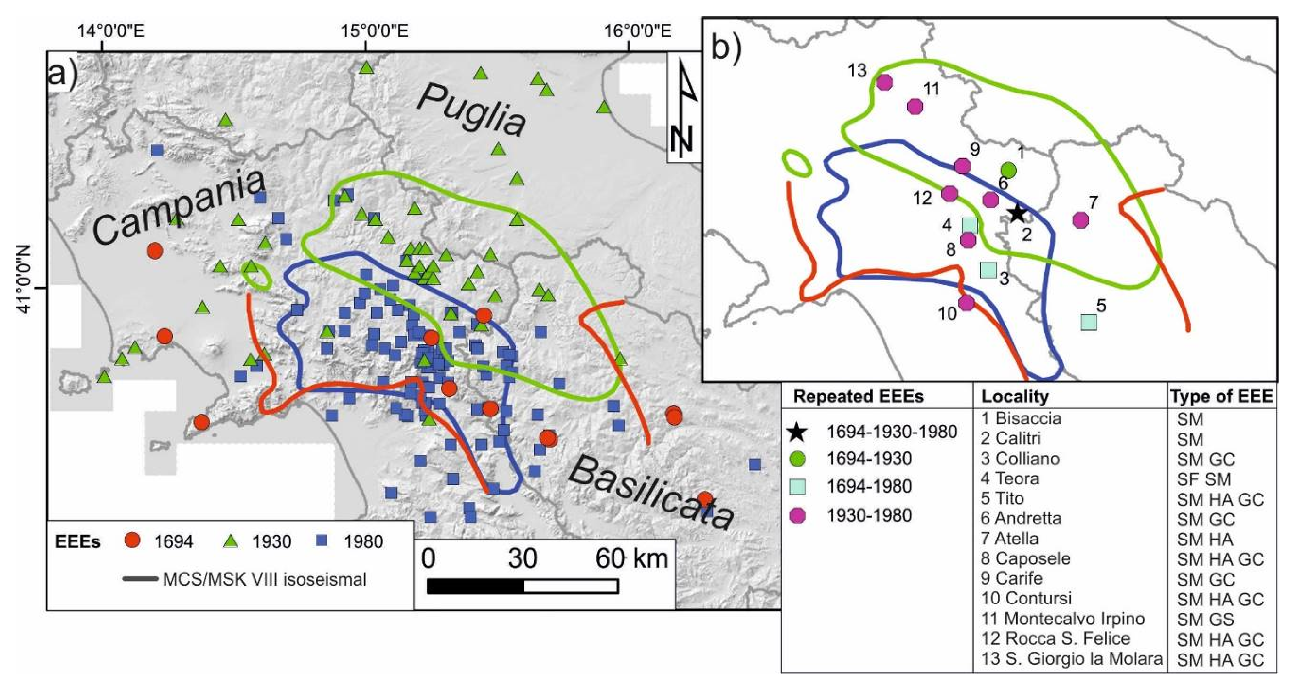
In Figure 3, we focus on three out of the five earthquakes (i.e., the 1694, 1930 and 1980 events [11,17,23,24,25,26,28,30]), because they all hit the area between Campania and Basilicata Regions. They shared a very similar magnitude (6.7–6.8), according to [14]. Figure 3a shows the EEEs together with the VIII isoseismal for the three earthquakes. The 1930 and 1980 events affected adjacent, partly overlapping areas. The VIII isoseismal was ca. 3900 and 2800 km2 wide for the 1930 and 1980 earthquakes, respectively. The VIII isoseismal for the 1694 earthquake broadly encompassed the area occupied by both the 1930 and 1980 isoseismals. EEEs for the 1694 earthquake were lower in number but spread over a much wider area. The percentages of EEEs inside the VIII isoseismal were 43%, 46% and 63% for the 1694, 1930 and 1980 earthquakes, respectively. Most of the environmental effects outside the VIII isoseismal were hydrogeological anomalies for the 1930 earthquake and slope movements for the 1980 one.
In Figure 3b, the localities hit by at least two out of the three earthquakes are reported, for a total of 13 localities. This figure is particularly relevant for the 1694 earthquake: in fact, five out of the 14 localities where EEEs were reported (i.e., 36%) were affected again by the 1930 and/or 1980 earthquakes. A total of 16% of the localities with documented EEEs in 1930 were affected by the 1980 earthquake. The only place where EEEs were documented for all the three earthquakes is Calitri. Following the 1980 earthquake, a rotational landslide of over 23 million m3 affected the historical center of the village; liquefaction phenomena were observed as well [17]. The seismic history of Calitri shows that the village was repeatedly hit by earthquakes and that landslides occurred also during the 1805 earthquake [32].
If we analyze the type of EEEs documented at the 13 localities, the most striking observation is that all were affected by slope movements; to a lesser extent ground cracks and hydrogeological anomalies were recorded. Local site conditions (physiography, geomorphological or lithological setting) influence the occurrence of EEEs, which tend to repeat at the same spot (e.g., [31,33]).
4.2. Quantitative Comparison of MCS/MSK and ESI Macroseismic Fields
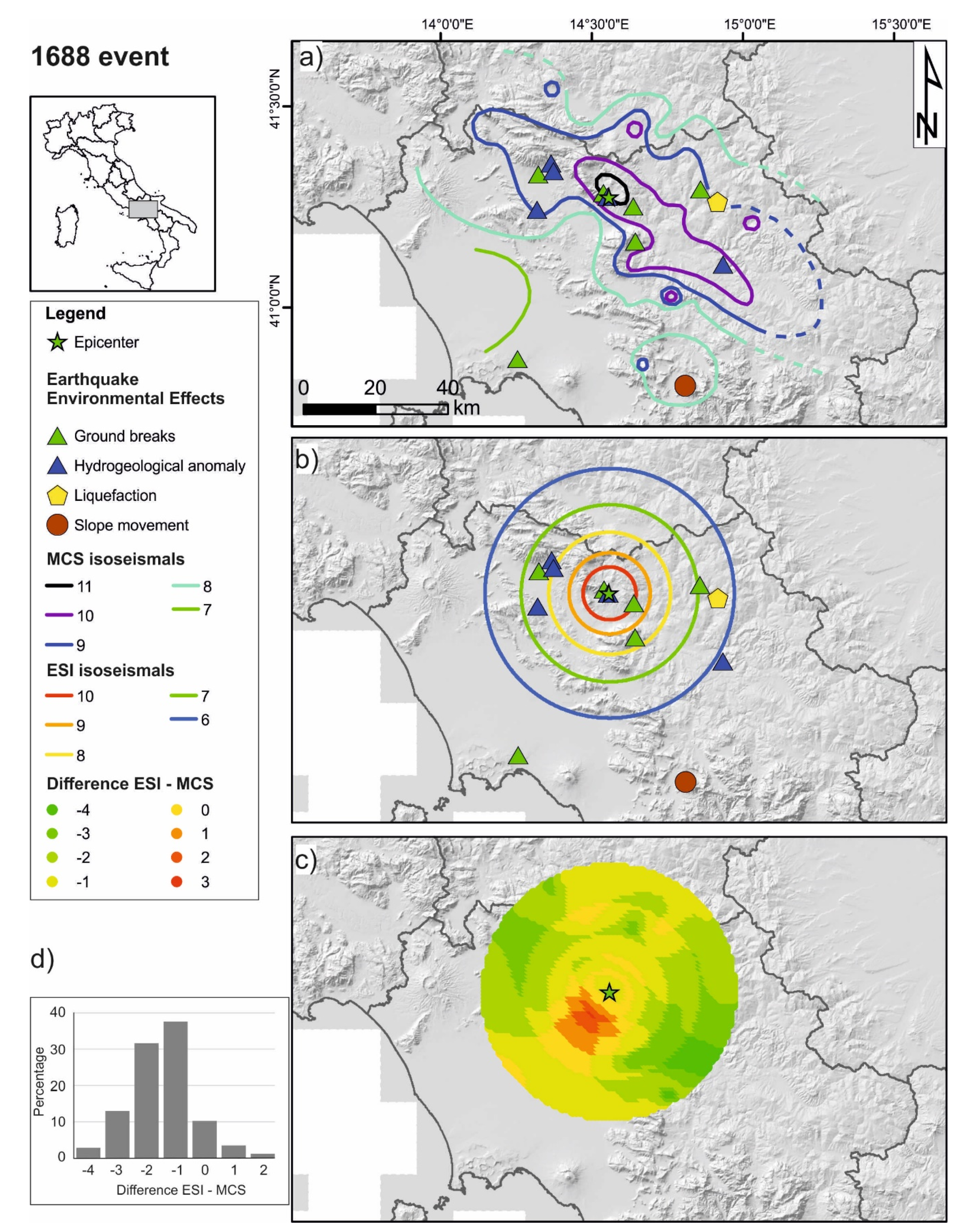
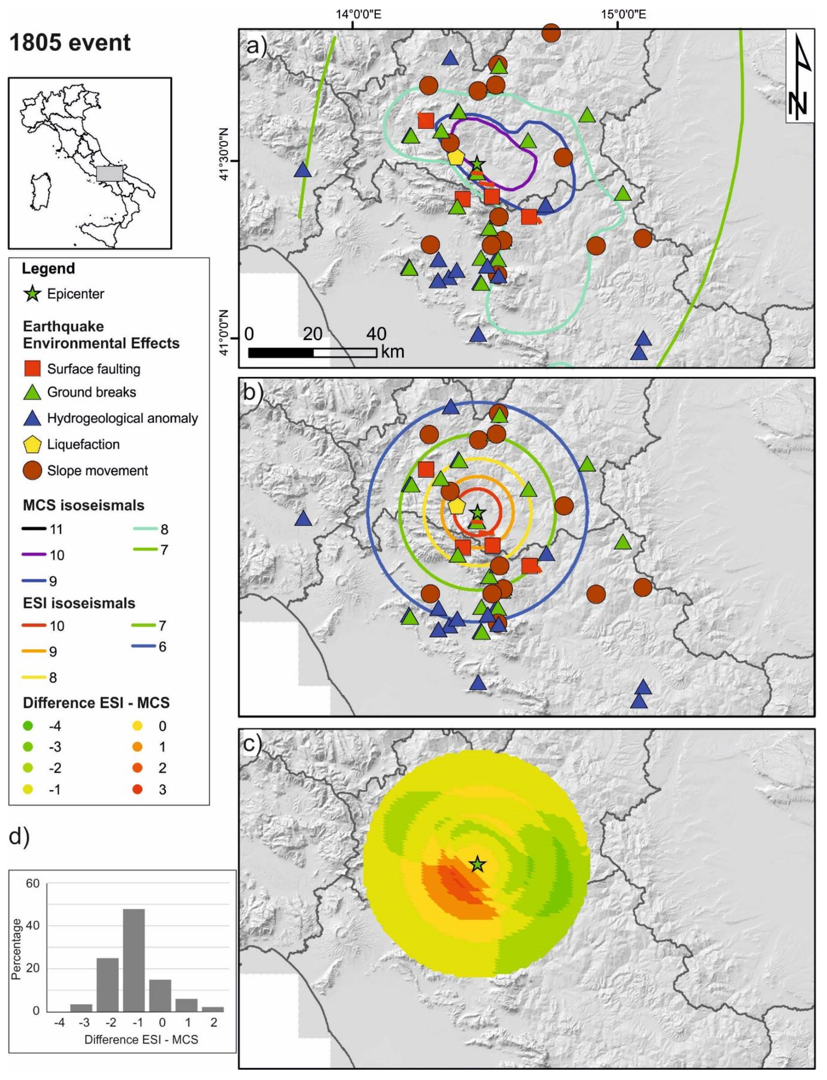
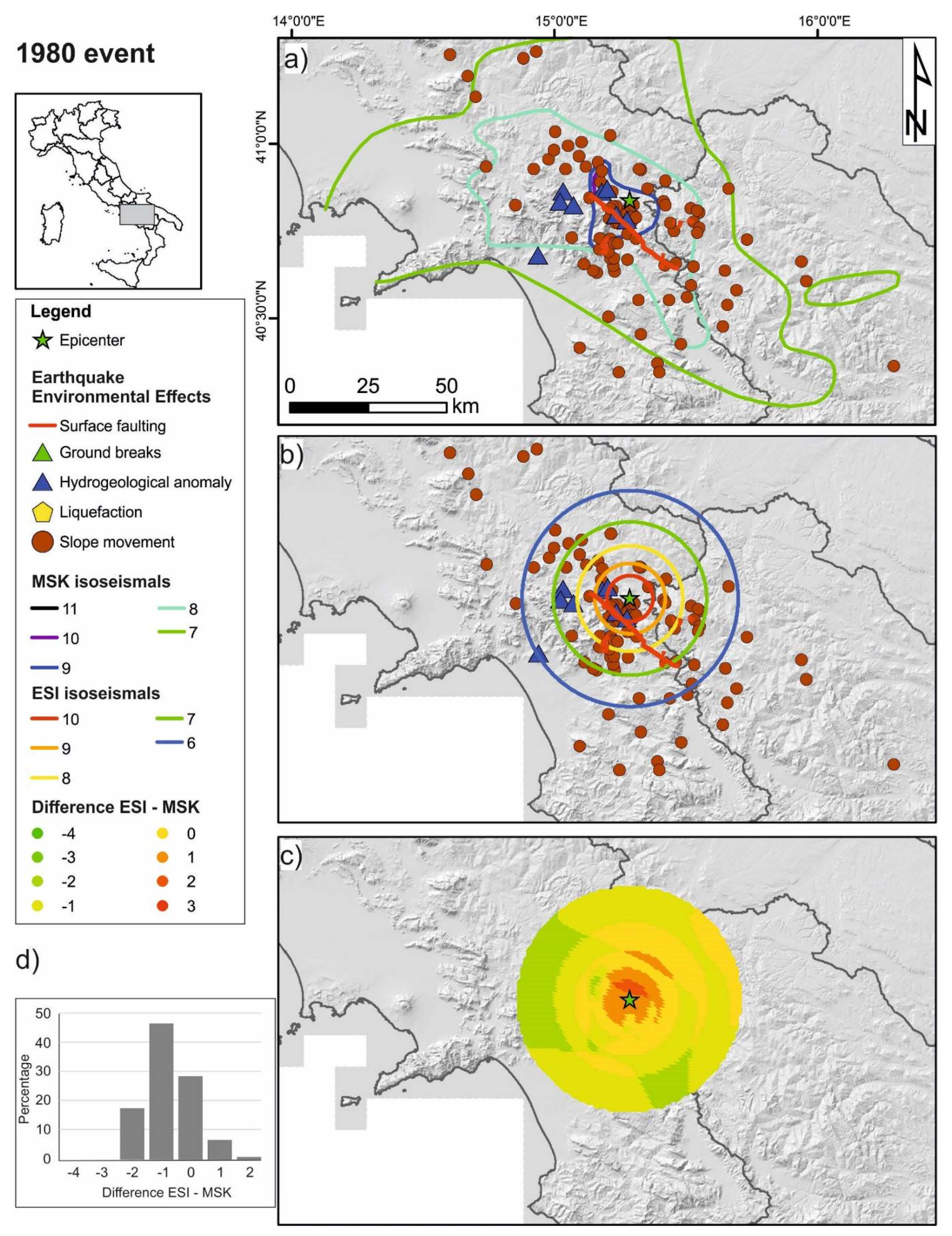
We now move toward a comparison of the earthquake effects on the natural environment (ESI scale) with the built environment (MCS and MSK scales). We considered each of the five historical earthquakes at a time and compare the distribution of EEEs and the value and pattern of macroseismic fields. Figure 4, Figure 5, Figure 6, Figure 7 and Figure 8 show the obtained results for each earthquake. In the upper panel, the location of EEEs is shown together with the MCS or MSK macroseismic field. For all the earthquakes, isoseismals are elongated in the NW–SE direction, in accordance with the strike of the main Apennines faults. The seismogenic faults of the older earthquakes have not been unequivocally identified so far; despite this fact, the anisotropy of isoseismals suggests the activation of NW–SE oriented sources.
The ESI macroseismic field derived from the intensity prediction equation is shown in the second panel of Figure 4, Figure 5, Figure 6, Figure 7 and Figure 8; the isoseismals are circular, since the IPE does not consider along- and across-strike anisotropies. ESI isoseismals occupy a much smaller area than MCS/MSK ones, due to the steep decay of ESI intensity moving away from the epicenter.
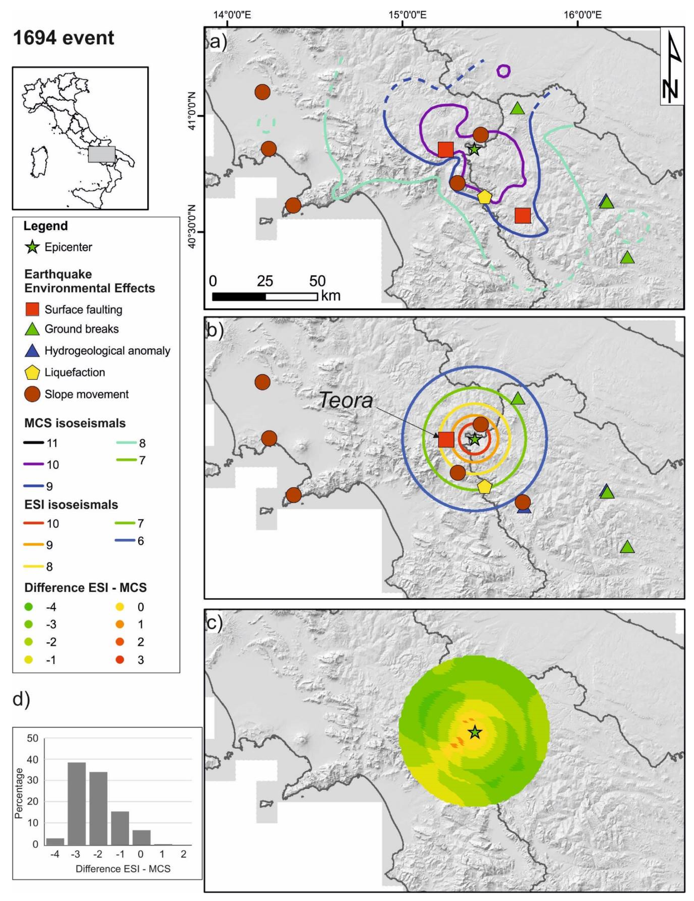
We calculated the difference between ESI and MCS intensities on a grid of 1 km2 cells and expressed this value as “ESI-MCS”. In Figure 4, Figure 5, Figure 6, Figure 7 and Figure 8 (panel c), red tones correspond to positive values of the “ESI-MCS” descriptor (i.e., ESI > MCS), while green tones correspond to negative values (i.e., MCS > ESI). Positive values are located closer to the epicenter; the frequency distribution of the “ESI-MCS” field is given in the histograms in the lower left corner of Figure 4, Figure 5, Figure 6, Figure 7 and Figure 8. For all the earthquakes, the mode corresponds to the value −1; the only exception is the 1694 seismic event, whose histogram (Figure 5d) looks shifted toward more negative values.
5. Discussion
5.1. The Significance of Macroseismic Historical Reading
Seismic sequences that occurred in the last few years showed a high degree of complexity in terms of spatio-temporal evolution of the sequence, number of ruptured segments and surficial expression of faulting. Earthquakes like the 2016 Central Italy [34], 2016 Kumamoto—Japan [35], 2016 Kaikoura—New Zealand [36], 2019 Ridgecrest—USA [37], to name just a few, were captured with unprecedented detail and enhanced our understanding of earthquakes and active tectonics. There is no reason why earthquakes that occurred in the past should not have been equally complex. The challenges we face today (variability in surface displacement, distributed faulting, cumulative effects on the natural and built environments) were even harder for past seismic events, due to the lower resolution of available data.
Thus, historical data bear a fundamental role and there is the need to reassess past earthquakes under a new light. For instance, the description of the environmental effects at Teora (see Figure 5b for location) in the 1694 earthquake is one of the first documentations of surface faulting associated with a linear morphogenic earthquake [38]: “The mountain split with great astonishment for a length of over 10 miles and the fracture was several arms wide, slowly decreasing toward the tip [La montagna con estrema meraviglia si è aperta per la lunghezza per lo spazio di 10 miglia sul dorso, essendo ampia l’apertura di più braccia, quale si va chiudendo a poco a poco.]” [28]. Another aspect usually encountered in historical seismicity data merits further attention: literary sources sometimes report church bell towers or mountain peaks that were visible from a nearby village before the earthquake and no more after (the contrary is also described many times). This indication may point toward the uplifting (or lowering) of large areas, as nowadays demonstrated by InSAR (Interferometric Synthetic Aperture Radar) data.
The 1694 and 1980 earthquakes were considered comparable in size and occurring from the same seismogenic source, due to the similarity in the distribution of damage [23]. Nevertheless, the VIII isoseismal of the 1694 earthquake (Figure 3a) was much bigger than the 1930 and 1980 earthquakes, as well as the area where EEEs were documented. Despite that the three earthquakes had a very similar magnitude in the most updated version of the Italian seismic catalogue (6.7–6.8, [14]), our observations possibly suggest that the size of the 1694 earthquake was bigger than the 1930 and 1980 earthquakes. This hypothesis seems to be confirmed by the much lower values of the “ESI-MCS” field for the 1694 earthquake (Figure 5d). An alternative explanation is that literary sources for older earthquakes tend to record extreme rather than “average” effects (e.g., [39]), which may lead to overestimation of the true size of the earthquake.
Macroseismic intensity assignment is based on a certain degree of expert judgement [1]; some authors considered the maximum observed effects, as in the original definition of the intensity parameter (e.g., [5]), while others preferred the average value [39]. We stress that this choice should be based on the specific needs: in some cases, the average scenario should be preferred; in other cases, it is necessary to consider the worst-case scenario and thus the maximum effects.
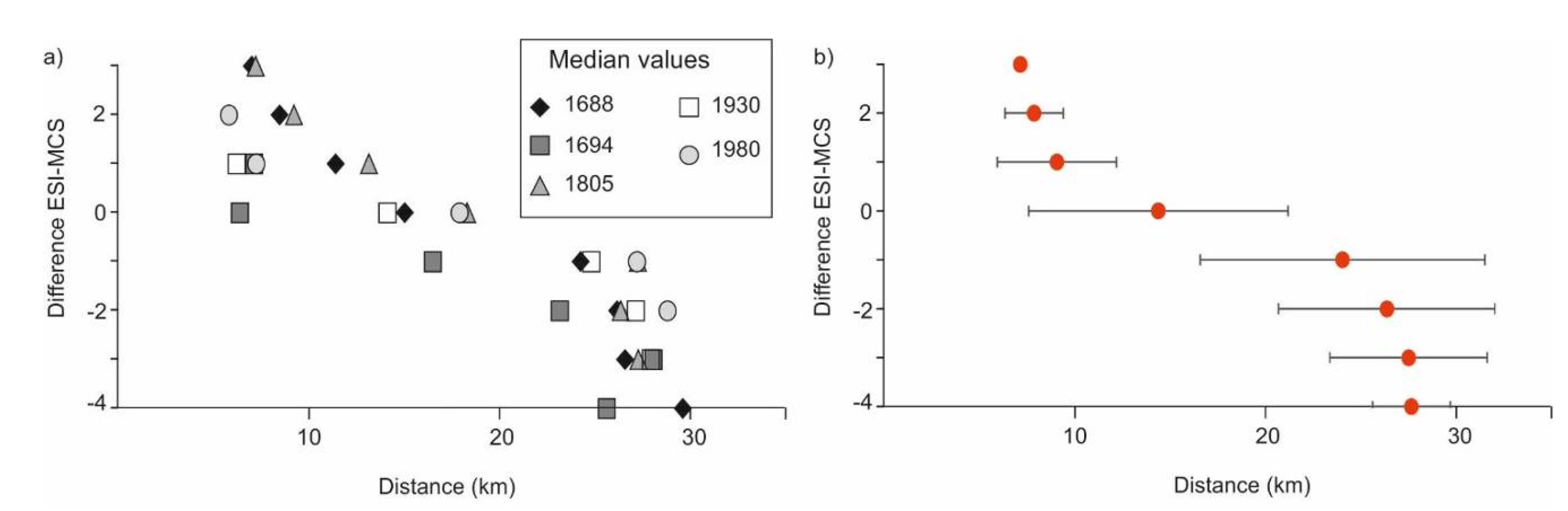
In Figure 9, we analyze the “ESI-MCS” field and plot it as a function of epicentral distance. At distances lower than 10 km, the ESI intensity is higher than MCS, while the opposite is true at distances higher than ca. 20 km. ESI and MCS have the same value at 14 ± 7 km from the epicenter. It must be recalled that we are not aiming at forcing the two scales to be equal, which would have no meaning; we simply want to highlight consistent features that can enable the comparison of different earthquakes. The higher steepness of the ESI attenuation [6] means that ESI is particularly useful in the near field [4,5], where traditional scales tend to saturate. A possible pitfall of the present analysis is that the earthquakes investigated in this research were already used for deriving the IPE: these results must be confirmed by analyzing independent case histories.
5.2. Environmental Effects and ESI Scale: Are They Reliable?
The number of EEEs documented for each of the five earthquakes ranges between 14 and 108 (see Table 1). This figure is well below the thousands of points available for the most recent earthquakes (e.g., over 4000 points for the 2016 Central Italy sequence [40]). This points toward a potential significant incompleteness of the data for older earthquakes (i.e., not all the localities where EEEs occurred are included in the reports); as a possible explanation, we argue that the careful search of ground effects has not been common practice until few years ago.
The number of documented EEEs for the five earthquakes analyzed in this study increased with time, indicating a better focusing on the ground effects produced by earthquakes. Even for the 1980 earthquake (EEEs reported for over 100 localities), the ESI scale was nonexistent; this means, in our opinion, that the adoption of the ESI involves, by default, a significant increase of the EEEs data, as demonstrated by the recent earthquakes in Italy (e.g., 2016 Central Italy seismic sequence [40,41]). We argue that the best practice for future earthquakes should include the adoption of both traditional scales and the ESI scale, because environmental effects may add a significant contribution in terms of seismic hazard assessment [5].
EEEs can be triggered at the same location by different seismic events (see Figure 3b), implying the presence of predisposing factors. In our opinion, this is a demonstration of the reliability of EEEs through time in a homogenous territorial setting. The repeatability of EEEs at the same location resembles one of the basic assumptions in earthquake geology, that is, tectonic reactivation of faults can occur only on existing active faults (i.e., no new faults are generated in the short term [42]).
Another point worth mentioning is that the attenuation of MCS intensity with distance is variable with time: 21st century earthquakes show a different behavior relative to older ones; on the contrary, the ESI attenuation was found to be more stable [6]. The introduction of the ESI scale is much more recent than traditional scales like the MCS; for this reason, available case histories documented through the ESI scale are not sufficient for developing empirical regressions with regional validity. A first attempt to relate ESI intensity and magnitude was performed in the Mediterranean region [43], whereas the only regression of ESI intensity with distance was developed in the Italian Apennines [6]. A possible improvement in the performance of ESI intensity prediction equation is the development of an anisotropic attenuation law, which takes into account the elongation of isoseismals in the direction of the seismogenic source (e.g., [44,45]).
6. Conclusions
In this study, we investigated the environmental effects triggered by five historical earthquakes that occurred in the Southern Apennines. We analyzed the spatial distribution of EEEs and their repeatability through time; we then compared the effects on the natural environment with the pattern of damage on the built environment, as documented by traditional intensity scales (MCS and MSK).
Our results demonstrated that EEEs are reliable indicators for determining the size and effects of past earthquakes; the reappraisal of literary sources under a modern perspective may help depicting a more detailed scenario of earthquake effects, thus providing improved input parameters for seismic hazard assessment. We argue that the reference practice in macroseismic assessment for future earthquakes should be to apply both the ESI and damage-based scales, which complement each other.
Author Contributions
Conceptualization, M.F.F. and L.S.; methodology, M.F.F.; software, M.F.F.; formal analysis, M.F.F. and L.B.; writing—original draft preparation, M.F.F.; writing—review and editing, L.S. and L.B. All authors have read and agreed to the published version of the manuscript.
Funding
This research received no external funding.
Acknowledgments
We want to thank Alessandro Michetti and Franz Livio (Insubria University) for fruitful discussion and Luca Guerrieri for providing us some of the EEE catalogue data.
Conflicts of Interest
The authors declare no conflict of interest.
Data and Resources
The ITHACA (ITaly HAzards from CApable faults) and DISS catalogues are available at http://sgi2.isprambiente.it/ithacaweb/default.aspx and http://diss.rm.ingv.it/diss/index.php/DISS321, respectively (last accessed July 2020) and were used to collect information on the active and capable faults. Data on the five earthquakes analyzed in the present study were collected from CPTI catalogue (epicentral coordinates, magnitude; https://emidius.mi.ingv.it/CPTI15-DBMI15/), CFTI (macroseismic effects; http://storing.ingv.it/cfti/cfti5/) and the EEE catalogue (environmental effects, http://193.206.192.211/wfd/eee_catalog/viewer.php); all were last accessed in July 2020.
References
- Cecić, I.; Musson, R. Macroseismic surveys in theory and practice. Nat. Hazards 2004, 31, 39–61. [Google Scholar] [CrossRef]
- Gaudiosi, G.; Nappi, R.; Alessio, G.; Porfido, S. Breve storia delle misurazioni dell’Intensità Macrosismica in Italia da Giuseppe Mercalli fino ai giorni nostri. Misc. INGV 2014, 24, 104–132, ISSN 2039–6651. [Google Scholar]
- Grunthal, G. European Macroseismic Scale 1998 (EMS-98). In Cahiers du Centre Europeen de Geodynamique et de Seismologie; Centre Europeen de Geodynamique et de Seismologie: Walferdange, Luxembourg, 1998; Volume 15, p. 99. [Google Scholar]
- Michetti, A.M.; Esposito, E.; Guerrieri, L.; Porfido, S.; Serva, L.; Tatevossian, R.; Vittori, E.; Audemard, F.; Azuma, T.; Clague, J. Intensity scale ESI 2007. In Memorie Descrittive della Carta Geologica d’Italia; Guerrieri, L., Vittori, E., Eds.; Servizio Geologico d’Italia Dipartimento Difesa del Suolo (ISPRA): Rome, Italy, 2007. [Google Scholar]
- Serva, L.; Vittori, E.; Comerci, V.; Esposito, E.; Guerrieri, L.; Michetti, A.M.; Mohammadioun, B.; Mohammadioun, G.C.; Porfido, S.; Tatevossian, R.E. Earthquake hazard and the environmental seismic intensity (ESI) scale. Pure Appl. Geophys. 2016, 173, 1479–1515. [Google Scholar] [CrossRef]
- Ferrario, M.F.; Livio, F.; Capizzano, S.S.; Michetti, A.M. Developing the First Intensity Prediction Equation Based on the Environmental Scale Intensity: A Case Study from Strong Normal-Faulting Earthquakes in the Italian Apennines. Seismol. Res. Lett. 2020. [Google Scholar] [CrossRef]
- Carrara, C.; Serva, L. Significato paleotettonico delle porzioni conglomeratiche di formazioni terrigene dell’Appennino meridionale. In Memorie della Società Geologica Italiana; Società geologica italiana: Roma, Italy, 1982; Volume 24, pp. 209–216. [Google Scholar]
- Cinque, A.; Patacca, E.; Scandone, P.; Tozzi, M. Quaternary kinematic evolution of the Southern Apennines. Relationships between surface geological features and deep lithospheric structures. Ann. Geophys. 1993, 36, 249–260. [Google Scholar]
- Doglioni, C.; Harabaglia, P.; Martinelli, G.; Mongeli, F.; Zito, G. A geodynamic model of the Southern Appennines accretionary prism. Terra Nova 1996, 8, 540–547. [Google Scholar] [CrossRef]
- Patacca, E.; Scandone, P. Geology of the Southern Apennines. Boll. Soc. Geol. It. 2007, 7, 75–119. [Google Scholar]
- DISS Working Group. Database of Individual Seismogenic Sources (DISS), Version 3.2.1: A Compilation of Potential Sources for Earthquakes Larger Than M 5.5 in Italy and Surrounding Areas. 2018. Available online: http://diss.rm.ingv.it/diss/ (accessed on 28 July 2020).
- ITHACA Working Group. ITHACA (ITaly HAzard from CApable faulting), A database of active capable faults of the Italian territory. Version December 2019. ISPRA Geological Survey of Italy. Available online: http://sgi2.isprambiente.it/ithacaweb/Mappatura.aspx (accessed on 28 July 2020).
- Guidoboni, E.; Valensise, G. On the complexity of earthquake sequences: A historical seismology perspective based on the L’Aquila seismicity (Abruzzo, Central Italy), 1315–1915. Earthq. Struct. 2015, 8, 153–184. [Google Scholar] [CrossRef] [Green Version]
- Rovida, A.; Locati, M.; Camassi, R.; Lolli, B.; Gasperini, P. Catalogo Parametrico dei Terremoti Italiani (CPTI15), Versione 2.0. Istituto Nazionale di Geofisica e Vulcanologia (INGV). Available online: https://doi.org/10.13127/CPTI/CPTI15.2 (accessed on 28 July 2020).
- Serva, L. Criteri geologici per la valutazione della sismicità: Considerazioni e proposte. Atti Convegni Lincei-Accad. Naz. Lincei 1995, 122, 103–116. [Google Scholar]
- Guidoboni, E.; Ferrari, G.; Tarabusi, G.; Sgattoni, G.; Comastri, A.; Mariotti, D.; Ciuccarelli, C.; Bianchi, M.G.; Valensise, G. CFTI5Med, the new release of the catalogue of strong earthquakes in Italy and in the Mediterranean area. Sci. Data 2019, 6, 80. [Google Scholar] [CrossRef]
- Porfido, S.; Esposito, E.; Vittori, E.; Tranfaglia, G.; Guerrieri, L.; Pece, R. Seismically induced ground effects of the 1805, 1930 and 1980 earthquakes in the Southern Apennines (Italy). Ital. J. Geosci. 2007, 333–346. [Google Scholar]
- Vilardo, G.; Nappi, R.; Petti, P.; Ventura, G. Fault geometries from the space distribution of the 1990–1997 Sannio-Benevento earthquakes: Inferences on the active deformation in Southern Apennines. Tectonophysics 2003, 363, 259–271. [Google Scholar] [CrossRef]
- Di Bucci, D.; Massa, B.; Zuppetta, A. Relay ramps in active normal fault zones: A clu to the identification of seismogenic sources (1688 Sannio earthquake, Italy). Geol. Soc. Am. Bull. 2006, 118, 430–448. [Google Scholar] [CrossRef]
- Nappi, R.; Alessio, G.; Bronzino, G.; Terranova, C.; Vilardo, G. Contribution of the SISCam Web-based GIS to the seismotectonic study of Campania (Southern Apennines): An example of application to the Sannio-area. Nat. Hazards 2007, 45, 73–85. [Google Scholar] [CrossRef]
- Nappi, R.; Alessio, G. Integrated morphometric analysis in GIS environment applied to active tectonic areas. In Earthquake Research and Analysis—Seismology, Seismotectonic and Earthquake Geology; InTechOpen: London, UK, 2012; ISBN 978-953-307-991-2. [Google Scholar]
- Blumetti, A.M.; Esposito, E.; Ferreli, L.; Michetti, A.M.; Porfido, S.; Serva, L.; Vittori, E. New data and reinterpretation of the November 23, 1980, M 6.9 Irpinia-Lucania earthquake (southern Apennines) coseismic surface effects. Stud. Geol. Camerti 2002. [Google Scholar] [CrossRef]
- Pantosti, D.; Schwartz, D.P.; Valensise, G. Paleoseismology along the 1980 surface rupture of the Irpinia Fault: Implications for earthquake recurrence in the Southern Apennines, Italy. J. Geophys. Res. 1993, 98, 6561–6577. [Google Scholar] [CrossRef]
- Westaway, R.; Jackson, J. Surface faulting in the southern Italian Campania-Basilicata earthquake of 23 November 1980. Nature 1984, 312, 436–438. [Google Scholar] [CrossRef]
- Esposito, E.; Porfido, S. Gli effetti cosismici sull’ambiente fisico per la valutazione della vulnerabilità del territorio. In Dalle Fonti all’Evento. Percorsi Strumenti e Metodi per L’analisi del Terremoto del 23 Luglio 1930 nell’Area del Vulture; Gizzi, F.T., Masini, N., Eds.; Edizioni Scientifiche Italiane: Naples, Italy, 2010; pp. 129–142. ISBN 978-88-495-2050-7. [Google Scholar]
- Serva, L.; Esposito, E.; Guerrieri, L.; Porfido, S.; Vittori, E.; Comerci, V. Environmental effects from five historical earthquakes in southern Apennines (Italy) and macroseismic intensity assessment: Contribution to INQUA EEE Scale Project. Quat. Int. 2007, 173–174, 30–44. [Google Scholar] [CrossRef]
- Serva, L. The earthquake of June 5, 1688 in Campania. In Atlas of Isoseismal Maps of Italian Earthquakes; Postpischl, D., Ed.; Consiglio Nazionale Ricerche—Progetto Finalizzato Geodinamica: Roma, Italy, 1985; Volume 114, pp. 44–45. [Google Scholar]
- Serva, L. The earthquake of September 8, 1694 in Campania- Lucania. In Atlas of Isoseismal Maps of Italian Earthquakes; Postpischl, D., Ed.; Consiglio Nazionale Ricerche—Progetto Finalizzato Geodinamica: Roma, Italy, 1985; Volume 114, pp. 50–51. [Google Scholar]
- Esposito, E.; Luongo, G.; Marturano, A.; Porfido, S. Il terremoto di S. Anna del 26 Luglio 1805. Mem. Soc. Geol. Ital. 1987, 37, 171–191. [Google Scholar]
- Spadea, M.C.; Vecchi, M.; Gardellini, P.; Del Mese, S. The Irpinia earthquake of July 23, 1930. In Atlas of Isoseismal Maps of Italian Earthquakes; Postpischl, D., Ed.; Consiglio Nazionale Ricerche—Progetto Finalizzato Geodinamica: Roma, Italy, 1985; Volume 114, pp. 136–137. [Google Scholar]
- Quigley, M.C.; Hughes, M.W.; Bradley, B.A.; van Ballegooy, S.; Reid, C.; Morgenroth, J.; Pettinga, J.R. The 2010–2011 Canterbury earthquake sequence: Environmental effects, seismic triggering thresholds and geologic legacy. Tectonophysics 2016, 672, 228–274. [Google Scholar] [CrossRef] [Green Version]
- Porfido, S.; Alessio, G.; Gaudiosi, G.; Nappi, R.; Spiga, E. The resilience of some villages 36 years after the Irpinia-Basilicata (Southern Italy) 1980 earthquake. In Proceedings of the 4th World Landslide Forum, Ljubiana, Slovenia, 30 May–2 June 2017; pp. 121–133. [Google Scholar]
- King, T.R.; Quigley, M.; Clark, D. Surface-rupturing historical earthquakes in Australia and their environmental effects: New insights from re-analyses of observational data. Geosciences 2019, 9, 408. [Google Scholar] [CrossRef] [Green Version]
- Chiaraluce, L.; Di Stefano, R.; Tinti, E.; Scognamiglio, L.; Michele, M.; Casarotti, E.; Cattaneo, M.; De Gori, P.; Chiarabba, G.; Monachesi, G.; et al. The 2016 Central Italy seismic sequence: A first look at the mainshocks, aftershocks, and source models. Seism. Res. Lett. 2017, 88, 1–15. [Google Scholar] [CrossRef]
- Shirahama, Y.; Yoshimi, M.; Awata, Y.; Maruyama, T.; Azuma, T.; Miyashita, Y.; Otsubo, M. Characteristics of the surface ruptures associated with the 2016 Kumamoto earthquake sequence, central Kyushu, Japan. Earth Planets Space 2016, 68, 1–12. [Google Scholar] [CrossRef] [Green Version]
- Hamling, I.J.; Hreinsdóttir, S.; Clark, K.; Elliott, J.; Liang, C.; Fielding, E.; D’Anastasio, E. Complex multifault rupture during the 2016 Mw 7.8 Kaikōura earthquake, New Zealand. Science 2017. [Google Scholar] [CrossRef] [PubMed] [Green Version]
- DuRoss, C.B.; Gold, R.D.; Dawson, T.E.; Scharer, K.M.; Kendrick, K.J.; Akciz, S.O.; Blair, L. Surface Displacement Distributions for the July 2019 Ridgecrest, California, Earthquake Ruptures. Bull. Seism. Soc. Am. 2020, 1–19. [Google Scholar] [CrossRef]
- Caputo, R. Ground effects of large morphogenic earthquakes. J. Geodyn. 2005, 40, 113–118. [Google Scholar] [CrossRef]
- Hough, S.E. Earthquake intensity distributions: A new view. Bull. Earthq. Eng. 2014, 12, 135–155. [Google Scholar] [CrossRef]
- Farabollini, P.; Angelini, S.; Fazzini, M.; Lugeri, F.R.; Scalella, G.; GeomorphoLab. La sequenza sismica dell’Italia centrale del 24 agosto e successive: Contributi alla conoscenza e la banca dati degli effetti di superficie. Rend. Online Soc. Geol. It. 2018, 46, 9–15. [Google Scholar] [CrossRef]
- Villani, F.; Civico, R.; Pucci, S.; Pizzimenti, L.; Nappi, N.; De Martini, P.M.; Agosta, F.; Alessio, G.; Alfonsi, L.; Amanti, M.A.; et al. A database of the coseismic effects following the 30 October 2016 Norcia earthquake in Central Italy. Sci. Data 2018, 5, 180049. [Google Scholar] [CrossRef] [Green Version]
- IAEA. The Contribution of Palaeoseismology to Seismic Hazard Assessment in Site Evaluation for Nuclear Installations; IAEA: Vienna, Austria, 2015; Available online: https://www-pub.iaea.org/MTCD/Publications/PDF/TE-1767_web.pdf (accessed on 28 July 2020).
- Papanikolaou, I.; Melaki, M. The environmental seismic intensity scale (ESI 2007) in Greece, addition of new events and its relationship with magnitude in Greece and the Mediterranean; preliminary attenuation relationships. Quat. Int. 2017, 451, 37–55. [Google Scholar] [CrossRef]
- Shebalin, N.V. Macroseismic data as information on source parameters of large earthquakes. Phys. Earth Planet. Int. 1973, 6, 316–323. [Google Scholar] [CrossRef]
- Teramo, A.; Stillitani, E.; Bottari, A. On an Anisotropic Attenuation Law of the Macroseismic Intensity. Nat. Hazards 1995, 11, 203–221. [Google Scholar] [CrossRef]
Figure 1.
(a) The map shows the epicenters of the five historical earthquakes studied (green stars, data from [14]) and the capable faults from Ithaca database [12]; (b) the workflow shows the steps of our analysis with the input data (yellow) and output data (green).

Figure 2.
Histograms of the frequency distribution of the five EEEs for each class of MCS/MSK intensity.
Figure 2.
Histograms of the frequency distribution of the five EEEs for each class of MCS/MSK intensity.

Figure 3.
Map (a) shows a comparison between the VIII isoseismals of the 1694, 1930 and 1980 earthquakes and the location of EEEs; map (b) shows the localities where EEEs were documented for more than one seismic event (SM: slope movement, GC: ground crack, SF: surface faulting, HA: hydrological anomaly, GS: ground settlement).

Figure 4.
(a) map of EEEs and MCS isoseismals, dashed when inferred, of the 1688 earthquake; (b) map of EEEs and ESI isoseismals derived from the intensity prediction equation (IPE); (c) map showing the difference between ESI and MCS intensities; (d) histogram of the ESI-MCS difference. Inset shows, in the grey rectangle, the study area in a larger map around Italy.

Figure 5.
(a) map of EEEs and MCS isoseismals, dashed when inferred, of the 1694 earthquake; (b) map of EEEs and ESI isoseismals derived from the intensity prediction equation (IPE); (c) map showing the difference between ESI and MCS intensities; (d) histogram of the ESI-MCS difference. Inset shows, in the grey rectangle, the study area in a larger map around Italy.

Figure 6.
(a) map of EEEs and MCS isoseismals of the 1805 earthquake; (b) map of EEEs and ESI isoseismals derived from the intensity prediction equation (IPE); (c) map showing the difference between ESI and MCS intensities; (d) histogram of the ESI-MCS difference. Inset shows, in the grey rectangle, the study area in a larger map around Italy.

Figure 7.
(a) map of EEEs and MCS isoseismals of the 1930 earthquake; (b) map of EEEs and ESI isoseismals derived from the intensity prediction equation (IPE); (c) map showing the difference between ESI and MCS intensities; (d) histogram of the ESI-MCS difference. Inset shows, in the grey rectangle, the study area in a larger map around Italy.

Figure 8.
(a) map of EEEs and MSK isoseismals of the 1980 earthquake; (b) map of EEEs and ESI isoseismals derived from the intensity prediction equation (IPE); (c) map showing the difference between ESI and MSK intensities; (d) histogram of the ESI- MSK difference. Inset shows, in the grey rectangle, the study area in a larger map around Italy.

Figure 9.
(a) Median values of the ESI-MCS field as a function of epicentral distance for each of the five historical earthquakes; (b) boxplots showing the mean value and standard deviation of the data shown in panel (a).
Figure 9.
(a) Median values of the ESI-MCS field as a function of epicentral distance for each of the five historical earthquakes; (b) boxplots showing the mean value and standard deviation of the data shown in panel (a).


Table 1.
Details of the analyzed earthquakes. Epicentral coordinates and magnitude (M) are from [14]; I0: epicentral intensity.
Table 1.
Details of the analyzed earthquakes. Epicentral coordinates and magnitude (M) are from [14]; I0: epicentral intensity.
| Date | Earthquake | Latitude | Longitude | M | I0 MCS /MSK | I0 ESI | Number of EEEs Localities | References |
|---|---|---|---|---|---|---|---|---|
| 05/06/1688 | Sannio | 41.283 | 14.561 | 7.1 | XI (MCS) | X | 15 | [26,27] |
| 08/09/1694 | Irpinia | 40.862 | 15.406 | 6.7 | X (MCS) | X | 14 | [26,28] |
| 26/07/1805 | Molise | 41.500 | 14.474 | 6.7 | X (MCS) | X | 49 | [17,26,29] |
| 23/07/1930 | Irpinia | 41.068 | 15.318 | 6.7 | X (MCS) | X | 57 | [25,26,30] |
| 23/11/1980 | Irpinia | 40.842 | 15.283 | 6.8 | X (MSK) | X | 108 | [11,17,23,24,26] |
Table 2.
Isoseismal radii obtained from the IPE (Intenstiy Prediction Equation, Equation (1)), considering an ESI epicentral intensity of X.
Table 2.
Isoseismal radii obtained from the IPE (Intenstiy Prediction Equation, Equation (1)), considering an ESI epicentral intensity of X.
| ESI Intensity | Isoseismal Radius (km) |
|---|---|
| X | 7.3 |
| IX | 11.2 |
| VIII | 16.8 |
| VII | 24.4 |
| VI | 34.4 |
© 2020 by the authors. Licensee MDPI, Basel, Switzerland. This article is an open access article distributed under the terms and conditions of the Creative Commons Attribution (CC BY) license (http://creativecommons.org/licenses/by/4.0/).
Share and Cite
MDPI and ACS Style
Ferrario, M.F.; Serva, L.; Bonadeo, L. Assessing the Reliability of Earthquake Environmental Effects in Historical Events: Insights from the Southern Apennines, Italy. Geosciences 2020, 10, 332. https://doi.org/10.3390/geosciences10090332
AMA Style
Ferrario MF, Serva L, Bonadeo L. Assessing the Reliability of Earthquake Environmental Effects in Historical Events: Insights from the Southern Apennines, Italy. Geosciences. 2020; 10(9):332. https://doi.org/10.3390/geosciences10090332
Chicago/Turabian StyleFerrario, Maria Francesca, Leonello Serva, and Livio Bonadeo. 2020. "Assessing the Reliability of Earthquake Environmental Effects in Historical Events: Insights from the Southern Apennines, Italy" Geosciences 10, no. 9: 332. https://doi.org/10.3390/geosciences10090332
Note that from the first issue of 2016, this journal uses article numbers instead of page numbers. See further details here.