Groundwater Storage Changes Derived from GRACE and GLDAS on Smaller River Basins—A Case Study in Poland

Faculty of Geoengineering, University of Warmia and Mazury in Olsztyn, 10-719 Olsztyn, Poland
*
Author to whom correspondence should be addressed.
Geosciences 2020, 10(4), 124; https://doi.org/10.3390/geosciences10040124
Submission received: 11 March 2020
/
Revised: 26 March 2020
/
Accepted: 27 March 2020
/
Published: 31 March 2020
(This article belongs to the Section Geophysics)
Abstract
:In the era of global climate change, the monitoring of water resources, including groundwater, is of fundamental importance for nature, agriculture, economy and society. The purpose of this paper is to check compliance of changes in groundwater level obtained from direct measurements in wells with groundwater storage (GWS) anomalies calculated using gravity recovery and climate experiment (GRACE) observations in Poland. Data from the global land data assimilation (GLDAS), in the form of soil moisture (SM) and snow water equivalence (SWE), were used to convert GRACE observations into a series of GWS changes. It was found that very high consistency occurs between GRACE observations and changes in water level in wells, while the GWS series obtained from GRACE and GLDAS do not provide adequate compatibility. Further research presented in the paper was devoted to attempts to explain this phenomenon. In addition, time series of GRACE, GLDAS and groundwater head series were analyzed.
1. Introduction
The gravity recovery and climate experiment (GRACE) mission operated from 2002 to 2017. In this 15+ year period, it provided a great deal of global observations of the mass distribution and flow, on and underneath the surface of the Earth. These observations explained many large scale processes connected with, among others, changes in polar ice, soil moisture, surface and ground water storage and ocean mass dynamics. GRACE observations have proved so valuable in many areas of earth science, that shortly after GRACE mission completion [1,2], another mission was initiated, called GRACE FO (gravity recovery and climate experiment follow-on) [3]. The principle of both missions is similar: measurements of satellite orbits, using GNSS (global navigation satellite systems) and laser tracking, are supplemented with very accurate measurements of the distance between two twin GRACE satellites.
We can distinguish three levels of GRACE observations:
- Raw measurement on Level-1 (L1),
- Geopotential in a form of a spherical harmonics coefficients on Level-2 (L2),
- Monthly values of a terrestrial water storage (TWS) on Level-3 (L3).
Calculation centers provide GRACE observations in a form of Release Notes, the newest version is RL06 [4]. In comparison to the latest version, the new one has improved corrections (tides, atmosphere and oceans). GRACE observations can be acquired from the three main computational centers, i.e., GFZ (GeoForschungsZentrum, Potsdam), CSR (Center for Space Research at University of Texas, Austin) and JPL (Jet Propulsion Laboratory). Data can be acquired in two forms: spherical harmonics coefficients and mascons. Spherical harmonics coefficient usage is the oldest method for geoid computation. It is based on extending harmonics up to a dedicated degree and order. Due to the fact that the model determined in such a way is very noisy, it needs spatial or temporal filtering. Noise can be observed in a final model, in the form of north–south stripes, so the model requires de-striping [5]—filters to remove errors, like averaging with Gaussian filtering, anisotropic non-symmetric filters or one of the anisotropic decorrelation filter a decision-directed Kalman - DDK filters (reducing the error stripes). The other method of model determination and presenting is a mascon technique—mass concentration computation. This alternative technique is designed as the native basis function, so every mascon has a known particular localization. An advantage of such a solution is that it does not need to be de-striped or smoothed. Moreover, due to the mascon approach, it is possible to easily separate land and ocean signals.
The gravity changes are caused by mass changes. These mass variations can be understood as a change in a very thin concentrated layer of water thickness (it means near the Earth’s surface). Usually, gravity changes are caused by water storage changes (in basins or the land hydrosphere, melting ice or mass exchange between an atmosphere and land/ocean). The vertical change caused by water mass change can then be recomputed into total water storage changes (TWS).
In many applications, the GRACE observations are combined with data from various land data assimilation systems, e.g., global land data assimilation (GLDAS), MERRA (modern era retrospective-analysis for research and applications) and climatic models. In the presented paper, the GLDAS model (the global land data assimilation system) was used [6,7].
The GLDAS aim is to gather both satellite and in situ data, together with advanced land surface modeling and data assimilation techniques [6]. GLDAS contains 28 types of data, such as a 1-km global vegetation dataset, soil and elevation parameters, observation-based precipitation and downward radiation products.
The global model simulations provided by GLDAS are widely used in many applications, e.g., weather and climate prediction, water resource applications and water cycle investigations. Simulations are provided in 1-degree and 0.25-degree resolution, from 1948 up to now in four sub-models, NOAH (National Centers for Environmental Prediction/Oregon State University/Air Force/Hydrologic Research Lab Model), CLM (community land surface models), VIC (variable infiltration capacity) and Mosaic.
After separation contributions to temporal mass changes, groundwater changes can be computed [8]. It is recommended to resolve water mass variability with GRACE, using a minimum region size of approximately 200,000 km2 [9]. The purpose of this paper is to verify the possibility of successfully using GRACE observations in smaller areas. The two largest Polish basins (Vistula and Odra) do not meet the requirements of [10]. The Vistula basin covers an area of about 194,500 km2, and the Odra basin covers about 118,900 km2.
There are many determinations of groundwater using satellite models and observations and comparison of these determinations with a terrestrial data. It was concluded in [11] that GRACE data can increase the correlation between satellite-based observations and well-groundwater data. It was also noted that when taking into account groundwater data from wells, GRACE observations strongly and positively impacts time series of groundwater storage.
Another application of both GRACE and well data for groundwater storage comparison was presented for the area of Alberta, Canada [12]. It was concluded that successful isolating the groundwater storage (GWS) component from the GRACE TWS is mostly dependent on the accuracy of the soil moisture and snow water values. Determining groundwater storage allowed the authors to notice that accurate final determination needs a dense distribution of terrestrial wells and realistic evaluation of a porosity coefficient at wells’ localization. Final results of comparison GRACE-derived GWS and 256 well data revealed that only 36 wells were significantly correlated with the GWS from GRACE (correlation coefficient of 0.68). A site factor (standard deviation ratio) at all the 36 wells is strongly dependent on geological patterns at the area [13].
The groundwater storage was also examined for Western India, in Rajasthan, where many contrasting patterns were observed when analyzing data—an increasing trend was observed for wells, while for GRACE derived groundwater storage the trend was negative, which resulted in a negative correlation of −0.14. On the other hand, when analyzing Gujarat, for well and GRACE observations the same pattern was noticed—a positive relationship of 0.64 [14].
In [15] a GWS determination in the areas of sparse hydrogeological databases (southern Mali, Africa) was presented—only 16 wells within the region. The analysis showed a strong correlation between the GRACE-derived GWS and those from direct well measurements. When GRACE data was corrected with the soil moisture, the magnitude and relative timing of groundwater-storage changes was predicted more accurately. Based on the research it was concluded that GRACE could become a valuable resource management tool in regions lacking hydrogeological data.
In the paper, the following procedure was applied: a deduction of GRACE TWS data to deeper water storage using GLDAS information and a comparison of results with water level variations in chosen Polish wells. The detailed procedure used was developed on the basis of the Level-3 Data Product User Handbook [4].
For validation, a groundwater level from measurement wells was taken. In situ measurements are carried out by the National Hydrogeological Service (Polish abbreviation: PSH). The PSH provides groundwater measurements of water quantity and quality, fulfilling the necessity of assessing the quantitative and chemical status of groundwater. Groundwater monitoring is very important in terms of water resource management and protection. Over 2000 measurement wells are located in the area of Poland. Monitoring of wells is carried out at different time scales, depending on their function. The water table measurement is performed every day at the first order hydrogeological stations; and once a week at the second order hydrogeological stations. In some of the first and second order hydrogeological stations, automatic measurements of the groundwater level were introduced. Diagnostic monitoring takes place every three years and covers the entire country. In the years between diagnostic monitoring, operational monitoring is carried out, during which uniform parts are sampled once or twice a year, threatened by failure to achieve good condition in the perspective of 2021 [16].
The subject of monitoring of equivalent parts of groundwater (EPG) according to division into 172 uniform parts and separated from the basis by appropriately selected criteria fragments: subparts EPG. Due to the geological and hydrogeological analysis for the most area of Poland and the fact that groundwater resources in EPG are in multilevel structures, monitoring of numerous aquifers, levels and stories are not possible. Therefore, levels and/or stories were grouped into three aquifers complexes, taking into account hydrogeological conditions, dynamics and pressure exerted on them. An aquifer complex is a levels’ set connected with each other with a specific characteristics, like: lithological (sand, sand–gravel), stratigraphic (quaternary–tertiary), structural (kw of the valleys and lowlands), chemical (kw of sweet water), etc. The first complex is a groundwater reaching low-permeable level where pumping takes from a few days up to several months. It is a complex with an unconfined table that corresponds to the first aquifer (FA defined for the purposes of developing the Hydrogeological Map of Poland (HMP) in the scale of 1:50,000). The complex fed directly by precipitation infiltration. They do not have to meet the conditions specified for useful aquifers, it is possible to isolate these waters from the surface in a small area with a discontinuous packet of poorly permeable formations of low thickness (e.g., <2 m). The second complex are aquifers with a confined table (deep waters), insulated from the upper surface by a packet of poorly permeable formations, of considerable thickness (e.g., 2 m), fed with water filtration from a higher level with an unconfined table. Infiltration takes up to hundreds of years. The third complex is the water of the lowest occurring or the lowest of the identified usable aquifers, contacting or being able to contact the lower occurring levels of salt water. This complex is at risk of salt water ascension (the so-called deep water in hydraulic contact with deep water, which are most often brines) [17,18].
In the presented paper only the first complex is taken into account.
The approach to obtaining a representative monitoring result for the examined wells requires taking into account: its purpose, size of the research area, complications of geological structure and hydrogeological conditions, type and strength of economy pressure [18]. From this point of view, the following were considered:
- Partial representativeness, first of all taking into account the structure and parameters of aquifers/aquifers, location of pressure foci and is mainly relevant for determining the optimal location and depth of the research point;
- Temporal representativeness taking into account the speed of hydrogeological processes, which is combined with determining the appropriate frequency of measurements and tests (sampling). Determination of the structure and density of the observation and research network, as well as indication of locations of monitoring points in the area of a particular JCWPd (in Polish: Jednolite częsci wód podziemnych–Groundwater plain parts) of the selected aquifer, took place so as to obtain spatial representativeness of the network.
For research points of groundwater table location and source efficiency as well as diagnostic chemical monitoring, because it applies to all JCWPd, the following densities were adopted in individual aquifers:
- At groundwater level or usable aquifer with unconfined water table (when there is no insulation from the area)—1 point per 500 km2, but not less than 3 points within JCWPd.
The aim of the study is to check compliance of changes in groundwater level obtained from direct measurements in wells with groundwater storage (GWS) anomalies calculated using GRACE observations in Poland.
2. Data Used for the Study
2.1. GRACE Data
The GRACE TWS data was obtained from the JPL NASA [19], in the form of monthly gravity mascon solutions with a CRI filter (a Coastline Resolution Improvement) applied [20,21].
The JPL mascon data are given with the resolution of 0.5° in cm of equivalent water height. In the calculations, data given monthly, for the period from November 2006 to October 2016 were used. Missing epochs were completed by linear interpolation using the “approx” function of R [22]. This procedure gave 120 epochs (months) of monthly data, referenced to the 15th day of each month. All of the GRACE data were optimized to reduce the leakage effect, using scaling factors given together with the mascon JPL data. It should be noted that GRACE data are given in the form of anomalies in relation to the average value obtained in the period from January 2004 to December 2009. Any other period can be used to calculate the anomaly. In this paper we changed the period against which anomalies were calculated for January 2007 to December 2012. This was due to the fact that we used data for the wells for the period November 2006 to October 2016. Conversion to an anomaly relative to the average of another period is very simple and involves subtracting the new average from all previous anomaly values.
2.2. GLDAS Data
As recommended by the Level-3 Data Product User Handbook [4], the GLDAS NOAH model with a resolution of 0.25° was used to estimate the total amount of water contained in the surface of the investigated area. Water content in soil was modeled to the depth of 2 m in this model. It is given in the form of the soil moisture (SM), which is a static value expressed in kg/m2, which can easily be recomputed to the equivalent water height in cm. Other forms of water contained in the surface of the terrain include water contained in snow and water contained in all plants growing in a given area. The first value is given in the NOAH model as snow water equivalent (SWE), and the second as canopy (CA). Units are the same as in the soil moisture. Total water content estimated within the NOAH model is the sum of SM, SWE and CA. As noted previously, this expresses all forms of water contained on and under the surface, to the depth of 2 m. The same period of 120 months as in the case of the GRACE data was used. From all the data, the averages January 2007 to December 2012 were removed, thus the data presented are anomalies comparable with the GRACE data. It is worth mentioning that the GLDAS model, in addition to the NOAH submodel, also contains three other land assimilation models: The community land model (CLM) [23], the mosaic (MOS) model [24] and the variable infiltration capacity (VIC) model [25]. The other models were used for the purpose of looking for the best correlation.
2.3. Polish Wells
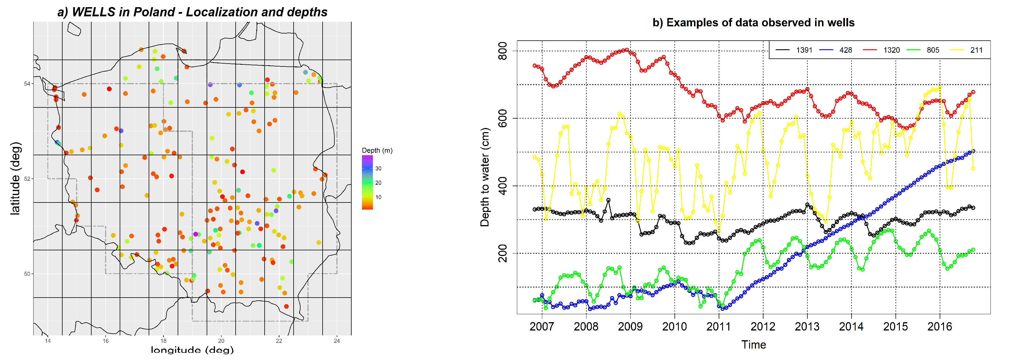
The groundwater level direct measurement data were obtained from the Polish Hydrogeological Annual Reports, from the years of 2007–2016 [26]. Above one thousand wells were reported, from which 215 wells were selected, only those that were continuously measured throughout the whole period of November 2006 to October 2016 (without gaps). When spatially averaging all time-series over the basins, 122 wells were assigned to the Vistula, 70 to the Odra basin and the remaining 23 were outside the basin areas (Figure 1a). It needs to be added that the average over the series may or may not give a good approximation of the real average of groundwater head series, so a possible bias due to the location needs to be taken into consideration.
Polish wells are very diversified, both due to the depth of the water surface and seasonal changes in level. Figure 1b shows some examples of the anomalies of the unconfined water level of chosen wells taken for calculations. Two wells were removed from the calculations, due to unusual behavior, like the well 428. It can be seen that depth variations of individual well levels differed significantly between each other. However, the calculated average variations for the Vistula and Oder basins were similar, see Figure 3. These resulting averages were adopted for comparisons with GWS and TWS in further parts of the paper. Let us remind that TWS stands for GRACE derived total water storage, while GWS stands for ground water storage computed based on TWS and GLDAS data, see Equation (1) below.
3. Methods
To work together with the GRACE and GLDAS data, we had to bring them to a uniform form. After unification of units to cm of equivalent water height, we must present the NOAH data in the form of anomalies in relation to the average for the period 2007.000–2012.999 and then aggregate the data to the coarser resolution of 0.5° of the GRACE data. To reduce resolution, the “aggregate” function from the R raster package was used [22,27].
Next, for all the raster cells and all the time epochs, the groundwater storage (GWS) anomalies were computed. It should be emphasized that all the water contained beneath the depth of 2 m, i.e., the water not taken into allowance in NOAH model, is referred to as the groundwater here. GWS was computed as the difference between the JPL GRACE TWS and the sum of GLDAS contents:
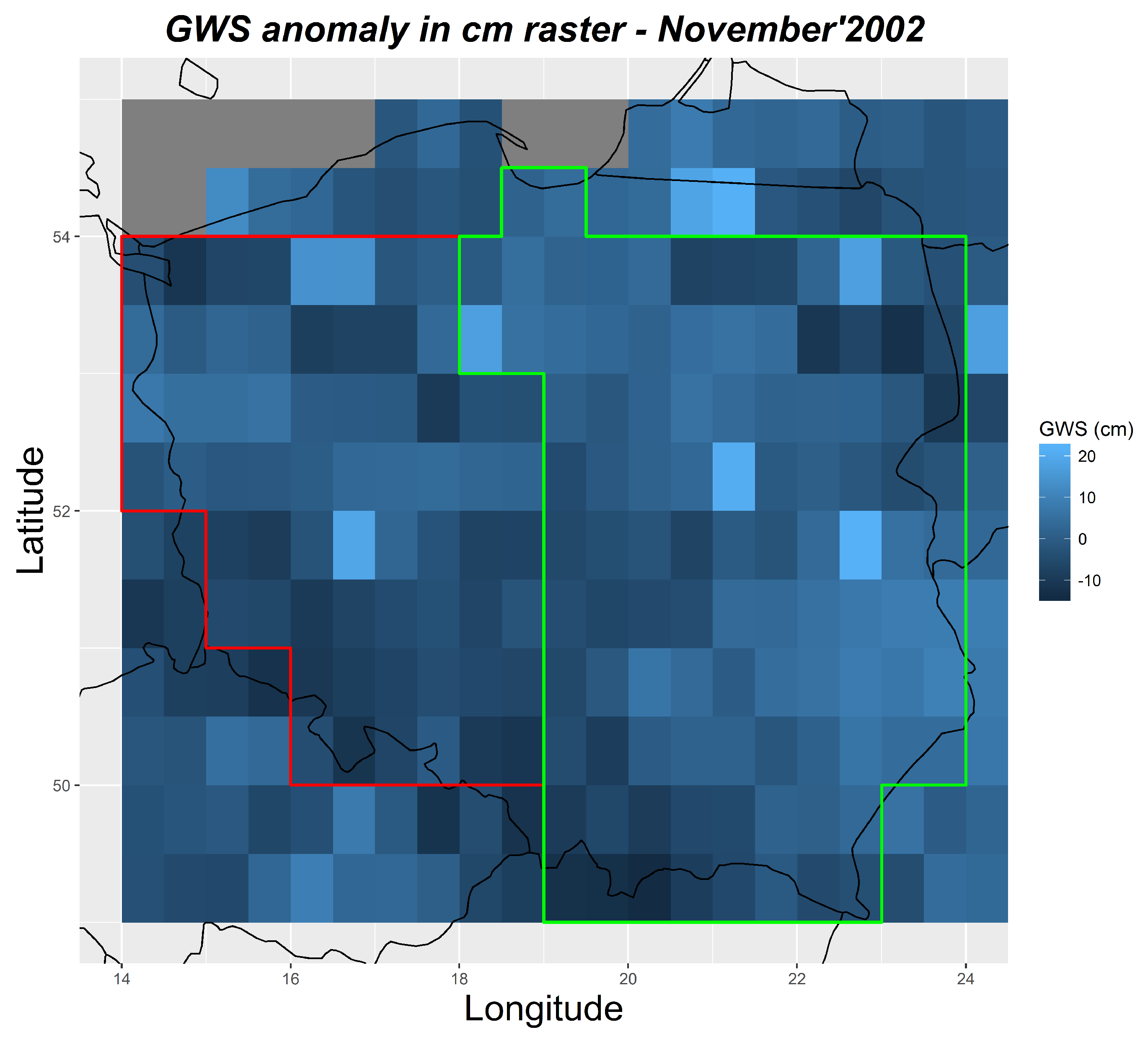
Units of all quantities in the above equation are cm of equivalent water height. The obtained raster of GWS data, for the first month taken for analyses, is given in Figure 2.
Next, the raster cell values were averaged over the generalized areas of Polish river basins (Vistula and Odra). The obtained means were further analyzed.
4. Analysis of Results
4.1. Comparison of GWS with Polish Well Data in 2006–2016
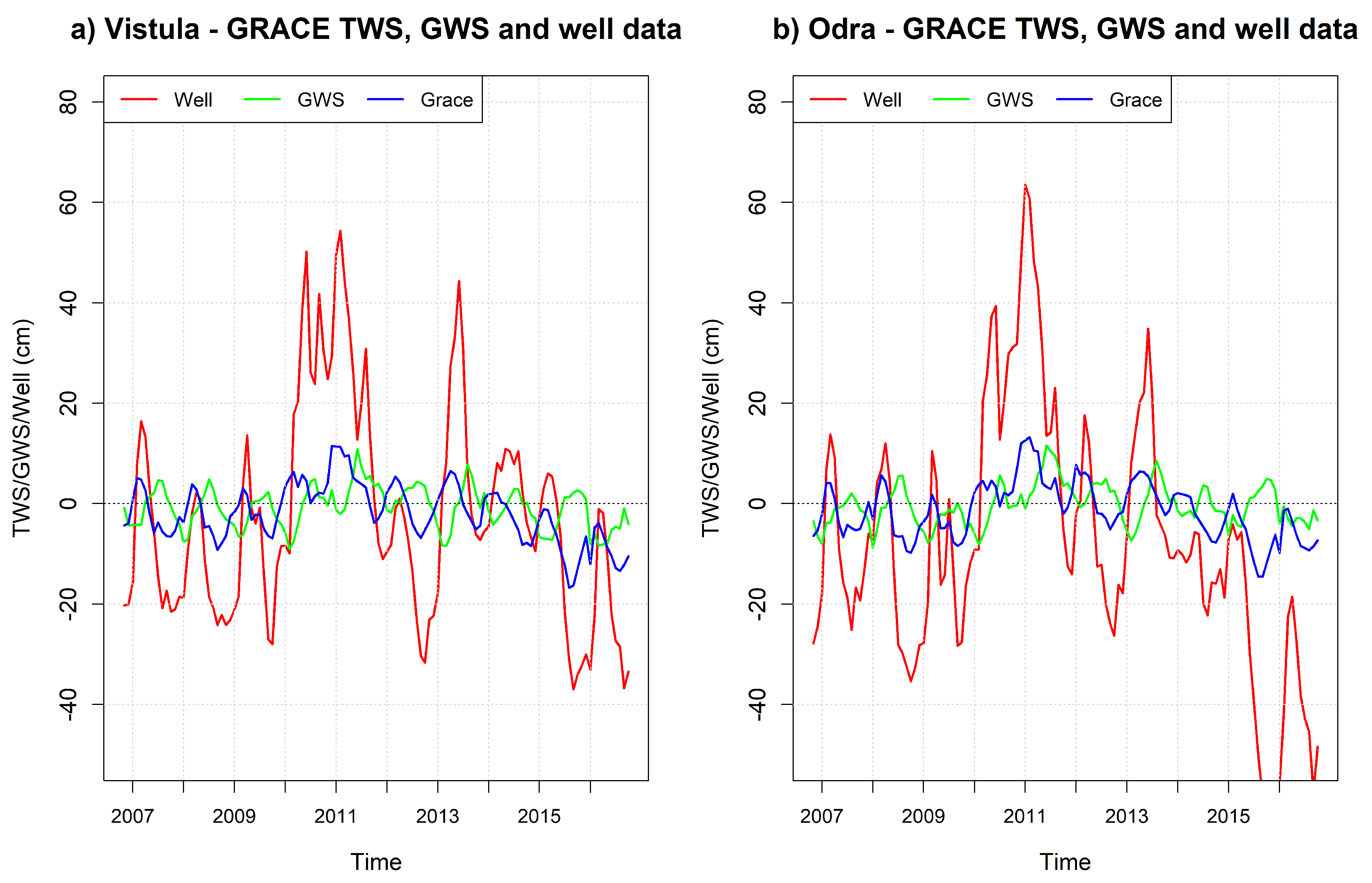
This analysis used data from 215 wells, located as presented in Figure 1a and covering the period of November 2006 to October 2016. The thicknesses of the unsaturated zone at the location of the well and GWS data averaged over the Vistula basin, Odra basin and over the total area of the two basins were compared. The time series of averaged data are plotted in Figure 3a,b.
It can be seen that the amplitudes of the thickness of the unsaturated zone at the location of the well changes were generally about four times greater than the amplitudes of the GRACE/NOAH GWS variations. A conclusion on the mean soil porosity can be derived: it was approximately equal to 0.25. This means that to raise the water level by an average of 1 cm on 1 square meter of the area, you need to pour 2500 cubic centimeters of water—instead of 10,000 cm3 in an empty space. This is only an approximate value due to the fact that information is lost when calculating the mean over the area. Thus, the obtained value of 0.25 can be considered as a conversion factor between the mean total storage (GWS) variation and the mean level (GWL) variation. The cross-correlations between the thickness of the unsaturated zone at the location of the well and GRACE/NOAH GWS variations were also computed. Maximum correlation between GWS and the thickness of the unsaturated zone at the location of the well is obtained for the time lag of three months for the both Vistula and Odra basins. Correlations between time series of the thickness of the unsaturated zone at the location of the well and GRACE TWS were much greater and less shifted, what is more, the shift is in a different direction. If a maximum of the mean thickness of the unsaturated zone at the location of the well occurs on June, then the appropriate maximum of GWS occurs in September, and that of GRACE in May. Shifts between GRACE and the thickness of the unsaturated zone at the location of the well seem more logical than between GWS and the thickness of the unsaturated zone at the location of the well: first, let us say in May, there is a lot of water (rain and humidity), then it soaks into the ground and causes (after one month, let us say in June) an increase of the water level in wells. However, it is much more difficult to explain the situation with GWS and the thickness of the unsaturated zone at the location of the well, when there is already a lot of water in the wells, and the calculated GWS reacts only after three months. It looks like the use of the NOAH model to convert GRACE TWS to GWS in Poland was not giving good results. Precise values of the cross-correlation functions (CCFs) are given in Table 1. Further analysis was aimed at finding an explanation of this phenomenon.
4.2. Analyses Concerning Well Depths
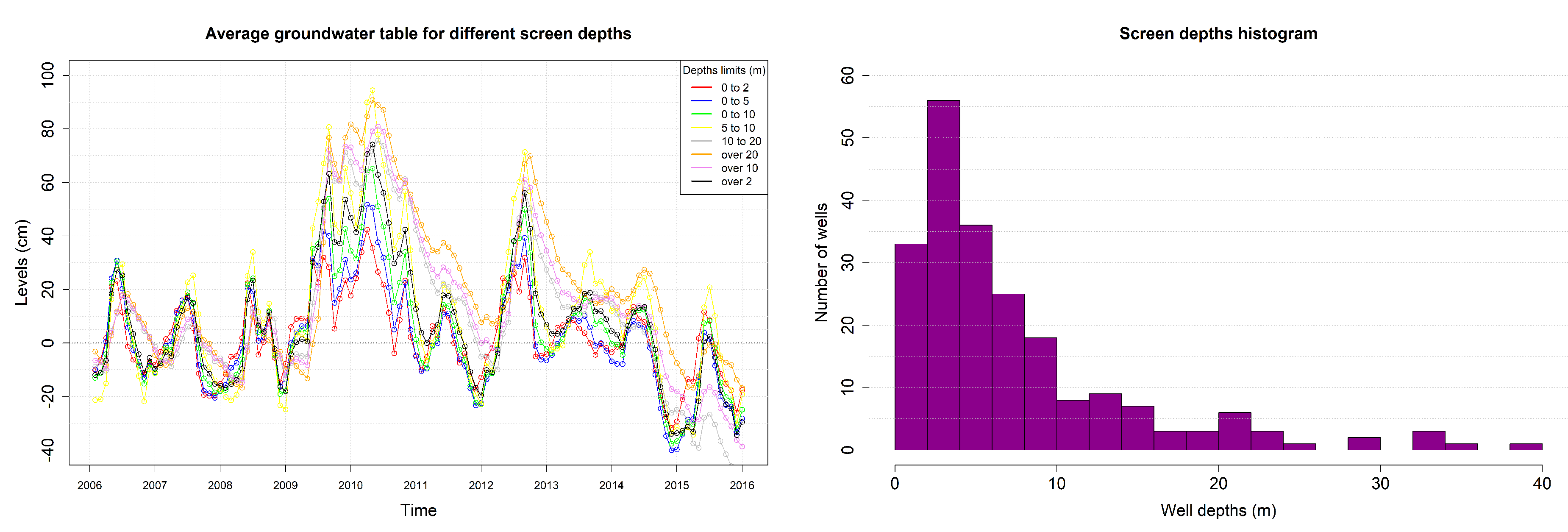
Firstly, it is worth examining the relationship of mutual time correlations between the thickness of the unsaturated zone at the location of the well, GWS, GRACE and the depth of the wells. As it was mentioned, NOAH models water content in soil (as the soil moisture, SM) to the depth of 2 m. In that case, acceptance of the thickness of the unsaturated zone at the location of the well only with depths greater than 2 m for averaging and comparison, should improve compatibility between GWS and the thickness of the unsaturated zone at the location of the well.
It can be seen from Figure 4a that time series of average thickness of the unsaturated zone at the location of the well changes for different depths were not shifted significantly. For example, the correlation coefficient calculated for wells up to 2 m deep and deeper than 2 m was 0.88. The maximum of CCF for these two groups of wells occurred at lag = −1 and was equal to 0.89. It suggests a very slight shift between the two time series, probably smaller than one month, and the direction of the shift was logical: deeper wells were delayed relative to shallower ones. The delay was probably less than one month.
In general, it can be summarized that despite the fact that the analyses were hindered by a different number of wells belonging to different depth ranges and by performing calculations on data with a monthly period when it is known that various changes can occur faster, it can be seen that differences in well depths causing differences in soaking time to these wells could not explain the 3-month shift between the GWS series and the thickness of the unsaturated zone at the location of the well. Based on Table 2, it can be concluded that the shifts between the thickness of the unsaturated zone at the location of the well and GWS were greater the shallower the wells were. Of course, it should be remembered that we were dealing with data whose annual signal was dominant, so a 4-month shift can be considered as an 8-month shift to the other direction. However, the analysis of Figure 3 rather contradicted this hypothesis. Shifts in such a way that GWS was on average about three months later, and for shallow wells even five months later than wells, were difficult to explain.
There were no such interpretation difficulties for the data from not reduced GRACE TWS. Firstly, the correlations in this study were much larger, and secondly, the shifts were in the right direction. For shallower wells (up to 2 m), the largest correlations were obtained for non-shifted series (rapid soaking/sinking), for deeper wells, the shift was one month (depth range from 2 to 10 m), and for even deeper (depths greater than 10 m) the shift amounted to two months. The shift direction was such that there was a maximum of TWS first, and then the water level in the wells increased. It can be seen that the deeper the wells, the longer the time of soaking water into them.
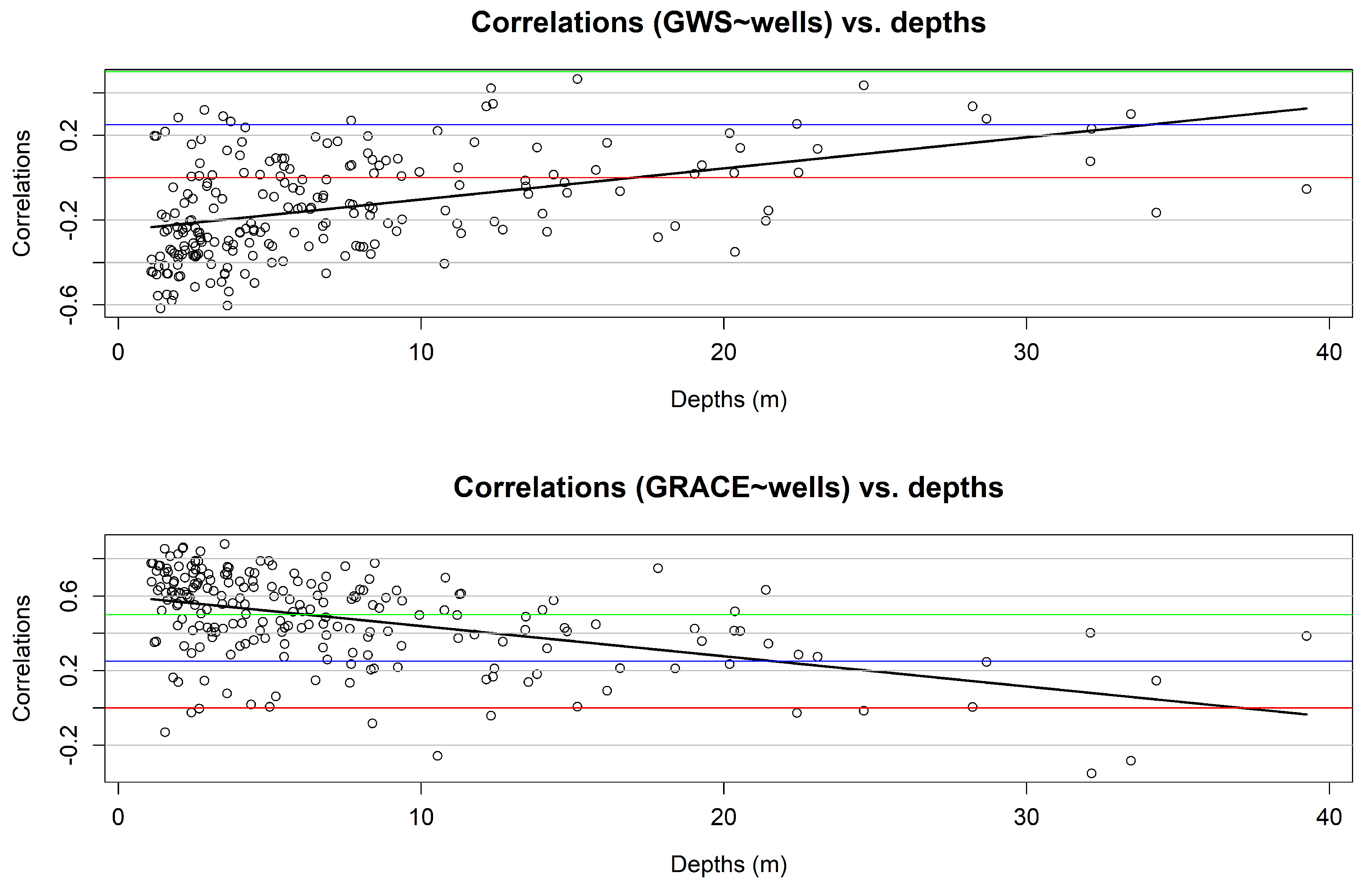
From Figure 5 it can be seen that there was a small correlation between the depth and the degree of correlation of the thickness of the unsaturated zone at the location of the well with GWS and GRACE, however, it can be seen that there was a large dispersion between the fitted regression line and the data. It is also seen that the correlations of GRACE versus the thickness of the unsaturated zone at the location of the well were much larger than the correlations of GWS versus the thickness of the unsaturated zone at the location of the well, and that most wells had depths less than 10 m, so that they had the greatest impact on the results. At any rate, it can be seen that GRACE better reflected the behavior of the water level in the wells than the GWS obtained from the merger of GRACE and NOAH [27,28].
4.3. Dependence on Localization
Changes in water conditions depend on climate conditions, the amount of water extraction for consumption, irrigation, industry and on the type of soil. Soil porosity (the sum of all free spaces in the soil) is of especially great importance for relations between the total water storage and the groundwater level.
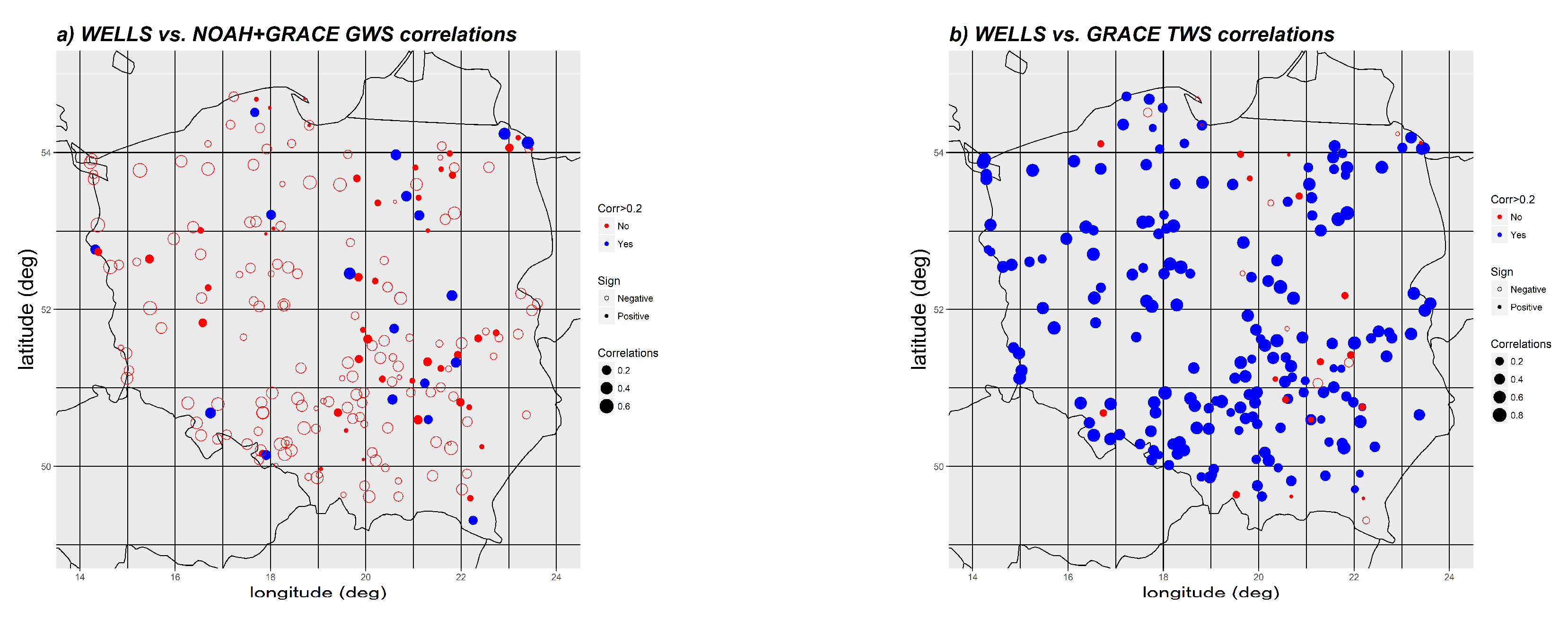
For the area of Poland, the porosity coefficient was estimated, e.g., in [29]. It obtained similar values in the Vistula and Odra basins (around 0.4). The two basin areas divide Poland into the eastern and western parts, while the different climate zones are rather arranged in latitudinal zones: in the south, there are mountains with more rainfall, in the north, the influence of the Baltic Sea is observed, which causes lower annual temperature amplitudes. To see if these changing climatic and soil conditions can affect the compatibility between the thickness of the unsaturated zone at the location of the well and GWS and the thickness of the unsaturated zone at the location of the well and GRACE, Figure 6 shows the correlations obtained on the area of Poland. Again, it can easily be seen that individual thickness of the unsaturated zone at the location of the well were very weakly correlated with a series of GWS changes, only a few thickness of the unsaturated zone at the location of the thickness of the unsaturated zone at the location of the well obtained correlations greater than 0.2, most thickness of the unsaturated zone at the location of the well have negative correlations (which was also visible in Figure 5). In contrast, compatibility between GRACE and individual wells was at a high level, only single wells have correlations less than 0.2. In both cases, no dependence on the location of the well can be seen. Thus, the local conditions surrounding the individual wells did not explain the lack of compliance (3-month shift) between the average changes in water level in the wells and the GWS series.
4.4. Dependence on the LDAS Model Admitted
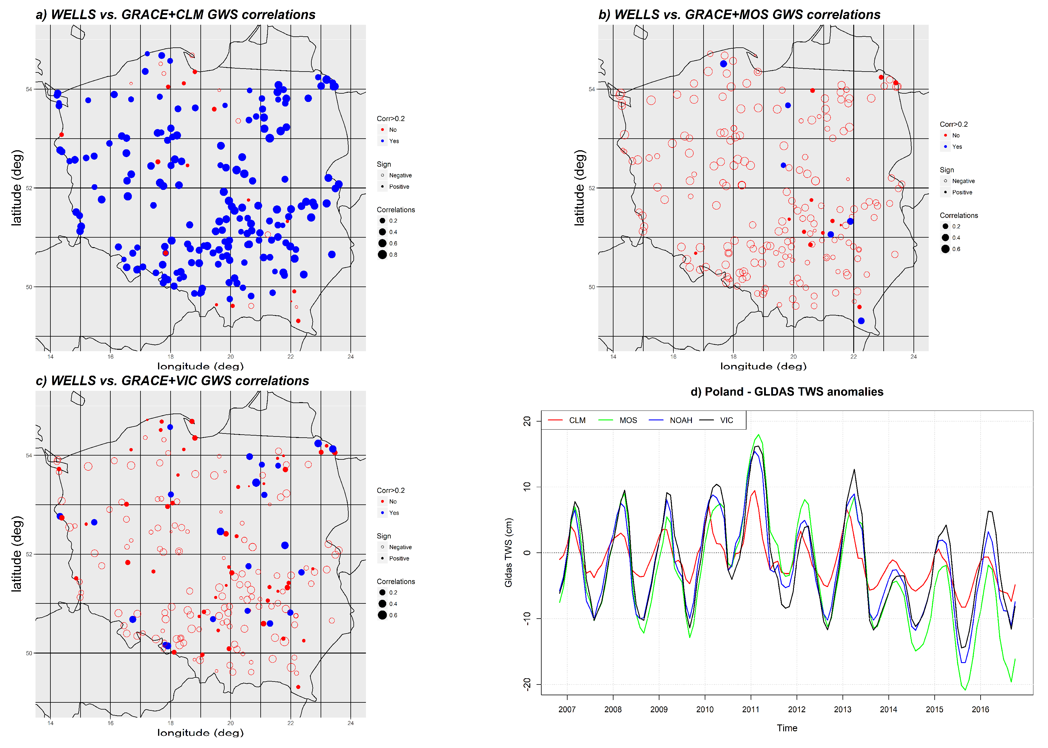
As already mentioned, the most recommended GLDAS model was NOAH but, in addition, there are three models available from NASA: CLM, MOS and VIC [30]. For completeness, the correlations obtained for the other three models were also examined, see Figure 7.
It can be seen in Figure 7 that the GWS results obtained were very different depending on which GLDAS model was used to convert GRACE TWS observations to groundwater head series. For MOS and VIC models, the correlations were very low, mostly negative. For CLM, the correlations were much greater, mostly positive and greater than 0.2. The correlation between GWS calculated from GRACE and CLM averaged over Poland and water level changes in wells, averaged over all wells, was equal to 0.74. It is, therefore, lower than the corresponding correlation coefficient for GRACE itself (see Table 1), but much higher than the correlations obtained based on other models.
Does it follow that the TWS calculated from CLM and NOAH is shifted between each other by some months? No, it can be seen from Figure 7d that the phase of GLDAS TWS changes from both models fit together very well, the correlation coefficient between them was 0.92. The problem lies in the amplitude of the changes—the amplitudes calculated from the NOAH model were much larger than the amplitudes obtained for the CLM model.
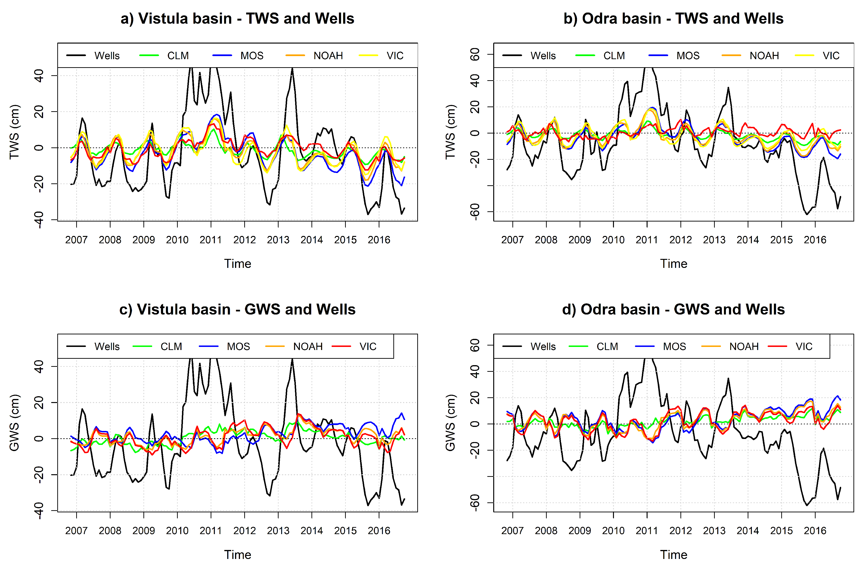
Let us recall the Equation (1), on the basis of which GRACE TWS is converted to GWS. In this equation, there is a difference between TWS from GRACE and TWS from the model admitted. In the case of differentiation of the time series, which have periodic components (in our case mainly annual), it is of great significance for the phase of the resulting signal, which are the magnitudes of the amplitudes of differentiated signals. If the amplitude of the NOAH annual changes were smaller, then the phase of the obtained GWS series would match the phase of mean well levels and GRACE TWS changes. The amplitudes of changes of the four examined models were different, which resulted in different phases of the GWS series obtained. It is well seen also in Figure 8.
5. Conclusions
- GRACE and the thickness of the unsaturated zone at the location of the well in Poland were highly correlated, wells data were delayed by one month on average. The cross-correlation function values were equal to 0.78 and 0.82 for Vistula and Odra basins at lag = 0, and to 0.82 and 0.90 respectively at lag = −1.
- After applying GLDAS NOAH to GRACE data, the resulting GWS were shifted in respect to direct measurements in wells by three months (GWS was delayed). The achieved values of the cross-correlation function were in this case much smaller (appropriate values were 0.20 and 0.21 for lag = 0, and 0.61 and 0.59 for lag = 3).
- No clear dependence of well depths and locations on the correlations could be observed.
- It seems that the GLDAS NOAH data had too large amplitudes of changes in comparison with the GRACE data on the area of the Polish basins studied.
- It seems that the CLM model fit much better in Poland for computation of groundwater storage variation values. Its annual amplitudes of changes were significantly smaller than the NOAH amplitudes. Due to this, the phase of TWS signal from GRACE did not change when performing differentiating according to Equation (1).
- However, it seems that GRACE data alone, not reduced by any model, when properly shifted, best reflected the behavior of the water level in the wells. The time shifts obtained between the GRACE series and the thickness of the unsaturated zone at the location of the well were logical and easy to interpret.
- It can be seen from the data that the changes in water levels in the wells were much greater than the changes in TWS from GRACE or GWS from GRACE and GLDAS. This is probably due to the mean soil porosity. Since the amplitudes of the thickness of the unsaturated zone at the location of the well changes were generally about four times greater than the amplitudes of the GRACE/NOAH GWS variations consequently a conclusion on the mean soil porosity could be derived: it was approximately equal to 0.25.
Author Contributions
Conceptualization, Z.R. and M.B.; methodology, Z.R. and M.B.; software, Z.R.; validation, Z.R. and M.B.; formal analysis, M.B.; investigation, Z.R. and M.B.; resources, M.B.; data curation, Z.R.; writing—original draft preparation, Z.R. and M.B.; writing—review and editing, Z.R. and M.B.; visualization, Z.R. and M.B.; supervision, Z.R. All authors have read and agreed to the published version of the manuscript.
Funding
This research received no external funding.
Conflicts of Interest
The authors declare no conflict of interest.
References
- Massoud, E.C.; Purdy, A.J.; Miro, M.E.; Famiglietti, J.S. Projecting groundwater storage changes in California’s Central Valley. Sci. Rep. 2018, 8, 1–9. [Google Scholar] [CrossRef] [PubMed]
- Purdy, A.J.; David, C.H.; Sikder, S.; Reager, J.T.; Chandanpurkar, H.A.; Jones, N.L.; Matin, M.A. An Open-Source Tool to Facilitate the Processing of GRACE Observations and GLDAS Outputs: An Evaluation in Bangladesh. Front. Environ. Sci. 2019, 7, 155. [Google Scholar] [CrossRef]
- Tapley, B.D.; Watkins, M.M.; Flechtner, F.; Reigber, C.; Bettadpur, S.; Rodell, M.; Sasgen, I.; Famiglietti, J.S.; Landerer, F.W.; Chambers, D.P.; et al. Contributions of GRACE to understanding climate change. Nat. Clim. Chang. 2009, 9, 358–369. [Google Scholar] [CrossRef] [PubMed]
- Cooley, S.S.; Landerer, F.W. GRACE D-103133 Gravity Recovery and Climate Experiment Follow-on (GRACE-FO) Level-3 Data Product User Handbook; NASA Jet Propulsion Laboratory, California Institute of Technology: Pasadena, CA, USA, 2019.
- Swenson, S.; Wahr, J. Post-processing removal of correlated errors in GRACE data. Hydrol. Land Surf. Stud. 2006, 36. [Google Scholar] [CrossRef]
- Rodell, M.; Houser, P.R.; Jambor, U.; Gottschalck, J.; Mitchell, K.; Meng, C.J.; Arsenault, K.; Cosgrove, B.; Radakovich, J.; Bosilovich, M.; et al. The Global Land Data Assimilation System. Bull. Amer. Meteor. Soc. 2004, 85, 381–394. [Google Scholar] [CrossRef] [Green Version]
- Liu, Z.; Liu, P.W.; Massoud, E.; Farr, T.G.; Lundgren, P.; Famiglietti, J.S. Monitoring Groundwater Change in California’s Central Valley Using Sentinel-1 and GRACE Observations. Geosciences 2019, 9, 436. [Google Scholar] [CrossRef] [Green Version]
- Rodell, M.; Famiglietti, J.S. The potential for satellite-based monitoring of groundwater storage changes using GRACE: The High Plains aquifer, Central US. J. Hydrol. 2002, 263, 245–256. [Google Scholar] [CrossRef] [Green Version]
- Rodell, M.; Famiglietti, J.S. An analysis of terrestrial water storage variations in Illinois with implications for the Gravity Recovery and Climate Experiment (GRACE). Water Resour. Res. 2001, 37, 1327–1339. [Google Scholar] [CrossRef] [Green Version]
- Rodell, M.; Famiglietti, J.S. Detectability of variations in continental water storage from satellite observations of the time dependent gravity field. Water Resour. Res. 1999, 35. [Google Scholar] [CrossRef] [Green Version]
- Li, B.; Rodell, M.; Kumar, S.; Beaudoing, H.K.; Getirana, A.; Zaitchik, B.F.; de Goncalves, L.G.; Cossetin, C.; Bhanja, S.; Mukherjee, A.; et al. Global GRACE Data Assimilation for Groundwater and Drought Monitoring: Advances and Challenges. Water Resour. Res. 2019, 5. [Google Scholar] [CrossRef] [Green Version]
- Huang, J.; Pavlic, G.; Rivera, A.; Palombi, D.; Smerdon, B. Mapping groundwater storage variations with GRACE: A case study in Alberta, Canada. Hydrogeol. J. 2016. [Google Scholar] [CrossRef] [Green Version]
- Meghwal, R.; Shah, D.; Mishra, V. On the Changes in Groundwater Storage Variability in Western India Using GRACE and Well Observations. Remote Sens. Earth Syst. Sci. 2019, 2, 741–755. [Google Scholar] [CrossRef]
- Henry, C.M.; Allen, D.M.; Huang, J. Groundwater storage variability and annual recharge using well-hydrograph and GRACE satellite data. Hydrogeol. J. 2011, 19. [Google Scholar] [CrossRef]
- Watkins, M.M.; Wiese, D.N.; Yuan, D.-N.; Boening, C.; Landerer, F.W. Improved methods for observing Earth’s time variable mass distribution with GRACE using spherical cap mascons. J. Geophys. Res. Solid Earth 2015, 120, 2648–2671. [Google Scholar] [CrossRef]
- Winter, T.C.; Harvey, J.W.; Lehn, O.; William, F.; William, M.A. Ground Water and Surface Water a Single Resource; U.S. Geological Survey Circular: Cantua Creek, CA, USA, 1998; Volume 1139.
- Witczak, S.; Kania, J.; Kmiecik, E. Katalog Wybranych Fizycznych I Chemicznych Wskaźników Zanieczyszczeń Wód Podziemnych I Metod Ich Oznaczania (Published in Polish: Catalog of Selected Types and Chemical Substances Contained in Groundwater and Methods of their Determination); Główny Inspektorat Ochrony Środowiska: Warszawa, Poland, 2013; ISBN 978-83-61227-13-7.
- Wiese, D.N.; Landerer, F.W.; Watkins, M.M. Quantifying and reducing leakage errors in the JPL RL05M GRACE Mascon solution. Water Resour. Res. 2016, 52. [Google Scholar] [CrossRef]
- R Core Team. R: A Language and Environment for Statistical Computing; R Foundation for Statistical Computing: Vienna, Austria, 2014; Available online: http://www.R-project.org/ (accessed on 12 December 2019).
- Available online: www.pgi.gov.pl (accessed on 21 December 2019).
- Oleson, K.W.; Lawrence, D.M.; Bonan, G.B.; Flanner, M.G.; Kluzek, E.; Lawrence, P.J.; Levis, S.; Swenson, S.C.; Thornton, P.E. Technical Description of Version 4.0 of the Community Land Model (CLM); NCAR Tech. Note NCAR/TN-478+STR; National Center for Atmospheric Research: Boulder, CO, USA, 2010; Available online: http://www.cesm.ucar.edu/models/cesm1.0/clm/CLM4_Tech_Note.pdf (accessed on 6 December 2019).
- Suarez, M.J.; Bloom, S.; Dee, D. Energy and Water Balance Calculations in the Mosaic LSM; NASA Technical Memorandum 104606; NASA: Greenbelt, MA, USA, 1996. Available online: https://gmao.gsfc.nasa.gov/pubs/docs/Koster130.pdf (accessed on 1 September 2019).
- Rodell, M.; Beaudoing, K.H. GLDAS VIC Land Surface Model L4 Monthly 1.0 x 1.0 degree V001; Goddard Earth Sciences Data and Information Services Center (GES DISC): Greenbelt, MA, USA, 2019. [CrossRef]
- Available online: https://disc.gsfc.nasa.gov/datasets/GLDAS_VIC10_M_001/summary?keywords=gldas%20vic (accessed on 20 December 2019).
- Sadurski, A. Hydrogeological Annual Reports. Polish Hydrological Survey; Hydrological Year 2015; Polish Geological Institute: Gdansk, Poland, 2016.
- Hijmans Robert, J. Introduction to the ’Raster’ Package (Version 3.0-2); 2019. Available online: https://cran.r-project.org/web/packages/raster/vignettes/Raster.pdf (accessed on 8 December 2019).
- Liang, J.; Yang, Z.; Lin, P. Systematic Hydrological Evaluation of the Noah-MP Land Surface Model over China. Adv. Atmos. Sci. 2019, 36, 1171–1187. [Google Scholar] [CrossRef]
- Pennemann, P.C.S.; Rivera, J.A.R.; Saulo, A.C.E.; Penalba, O.C.P. A Comparison of GLDAS Soil Moisture Anomalies against Standardized Precipitation Index and Multisatellite Estimations over South America. J. Hydrometeorol. 2016, 16. [Google Scholar] [CrossRef]
- Sliwinska, J.; Birylo, M.; Rzepecka, Z.; Nastula, J. Analysis of groundwater and total water storage changes in Poland using GRACE observations, in-situ data, and various assimilation models. Remote Sens. 2019, 11, 2949. [Google Scholar] [CrossRef]
- Available online: https://ldas.gsfc.nasa.gov/gldas (accessed on 12 November 2019).
Figure 1.
Polish well localization and approximate depths (a) and example depths variations (b).

Figure 2.
Groundwater storage (GWS) raster computed for November 2002, with marked areas used for averaging (green: Vistula basin, red: Odra basin).
Figure 2.
Groundwater storage (GWS) raster computed for November 2002, with marked areas used for averaging (green: Vistula basin, red: Odra basin).

Figure 3.
Average thickness of the unsaturated zone at the location of the well, gravity recovery and climate experiment (GRACE)/NOAH GWS and GRACE terrestrial water storage (TWS) anomalies on the area of Vistula basin (a) and Odra basin (b).
Figure 3.
Average thickness of the unsaturated zone at the location of the well, gravity recovery and climate experiment (GRACE)/NOAH GWS and GRACE terrestrial water storage (TWS) anomalies on the area of Vistula basin (a) and Odra basin (b).

Figure 4.
Average groundwater head for 6 different classes of screen depth (a) and number of wells with different depths (b).
Figure 4.
Average groundwater head for 6 different classes of screen depth (a) and number of wells with different depths (b).

Figure 5.
Correlations versus well depths: between GWS and the thickness of the unsaturated zone at the location of the well (a) and between GRACE and the thickness of the unsaturated zone at the location of the well (b).
Figure 5.
Correlations versus well depths: between GWS and the thickness of the unsaturated zone at the location of the well (a) and between GRACE and the thickness of the unsaturated zone at the location of the well (b).

Figure 6.
Correlations between the thickness of the unsaturated zone at the location of the well and GWS (a) and the thickness of the unsaturated zone at the location of the well and GRACE (b).
Figure 6.
Correlations between the thickness of the unsaturated zone at the location of the well and GWS (a) and the thickness of the unsaturated zone at the location of the well and GRACE (b).

Figure 7.
Correlations between the thickness of the unsaturated zone at the location of the well variations and GWS series obtained based on the community land model (CLM; a), the mosaic (MOS; b) and variable infiltration capacity (VIC; c) models of global land data assimilation (GLDAS); (d) shows GLDAS TWS = soil moisture (SM) + snow water equivalent (SWE) + canopy (CA) from the four GLDAS models.

Figure 8.
Well data compared to GRACE and GLDAS TWS (a,b) and to GWS (c,d).


Table 1.
Cross-correlation function (CCF) values between the thickness of the unsaturated zone at the location of the well and GWS or GRACE TWS values.
Table 1.
Cross-correlation function (CCF) values between the thickness of the unsaturated zone at the location of the well and GWS or GRACE TWS values.
| CCF Values | Vistula Basin | Odra Basin |
|---|---|---|
| CCF(GWS~wells) at lag = 0 | 0.20 | 0.21 |
| Max CCF(GWS~wells) = CCF(GWS~wells) at lag = 3 | 0.61 | 0.59 |
| CCF(GRACE~wells) at lag = 0 | 0.78 | 0.89 |
| Max CCF(GRACE~wells) = CCF(GRACE~wells) at lag = −1 | 0.82 | 0.90 |
Table 2.
Correlation of the thickness of the unsaturated zone at the location of the well variations with changes of GWS (GRACE/NOAH) and TWS (GRACE alone).
Table 2.
Correlation of the thickness of the unsaturated zone at the location of the well variations with changes of GWS (GRACE/NOAH) and TWS (GRACE alone).
| Depths (m) | No. of Wells | Cor(GWL ~well)[0] | Lag[max], Max | Cor(TWS ~well)[0] | Lag[max], Max |
|---|---|---|---|---|---|
| 0 ÷ 2 | 30 | −0.17 | 5 (0.61) | 0.88 | 0 (0.88) |
| Over 2 | 161 | 0.27 | 3 (0.62) | 0.82 | −1 (0.86) |
| 2 ÷ 5 | 68 | 0.06 | 4 (0.61) | 0.86 | −1 (0.86) |
| 5 ÷ 10 | 54 | 0.25 | 3 (0.61) | 0.75 | −1 (0.82) |
| 10 ÷ 20 | 23 | 0.48 | 1 (0.55) | 0.71 | −2 (0.78) |
| Over 20 | 15 | 0.52 | 1 (0.56) | 0.62 | −2 (0.73) |
| 0 ÷ 5 | 99 | 0.02 | 4 (0.62) | 0.87 | 0 (0.87) |
| 0 ÷ 10 | 154 | 0.10 | 3 (0.61) | 0.75 | −1 (0.85) |
| Over 10 | 38 | 0.51 | 1 (0.57) | 0.68 | −2 (0.77) |
© 2020 by the authors. Licensee MDPI, Basel, Switzerland. This article is an open access article distributed under the terms and conditions of the Creative Commons Attribution (CC BY) license (http://creativecommons.org/licenses/by/4.0/).
Share and Cite
MDPI and ACS Style
Rzepecka, Z.; Birylo, M. Groundwater Storage Changes Derived from GRACE and GLDAS on Smaller River Basins—A Case Study in Poland. Geosciences 2020, 10, 124. https://doi.org/10.3390/geosciences10040124
AMA Style
Rzepecka Z, Birylo M. Groundwater Storage Changes Derived from GRACE and GLDAS on Smaller River Basins—A Case Study in Poland. Geosciences. 2020; 10(4):124. https://doi.org/10.3390/geosciences10040124
Chicago/Turabian StyleRzepecka, Zofia, and Monika Birylo. 2020. "Groundwater Storage Changes Derived from GRACE and GLDAS on Smaller River Basins—A Case Study in Poland" Geosciences 10, no. 4: 124. https://doi.org/10.3390/geosciences10040124
Note that from the first issue of 2016, this journal uses article numbers instead of page numbers. See further details here.