Soil Water Content Diachronic Mapping: An FFT Frequency Analysis of a Temperature–Vegetation Index

 , ,
, ,  ,
, 
Abstract
:1. Introduction
2. Materials and Methods
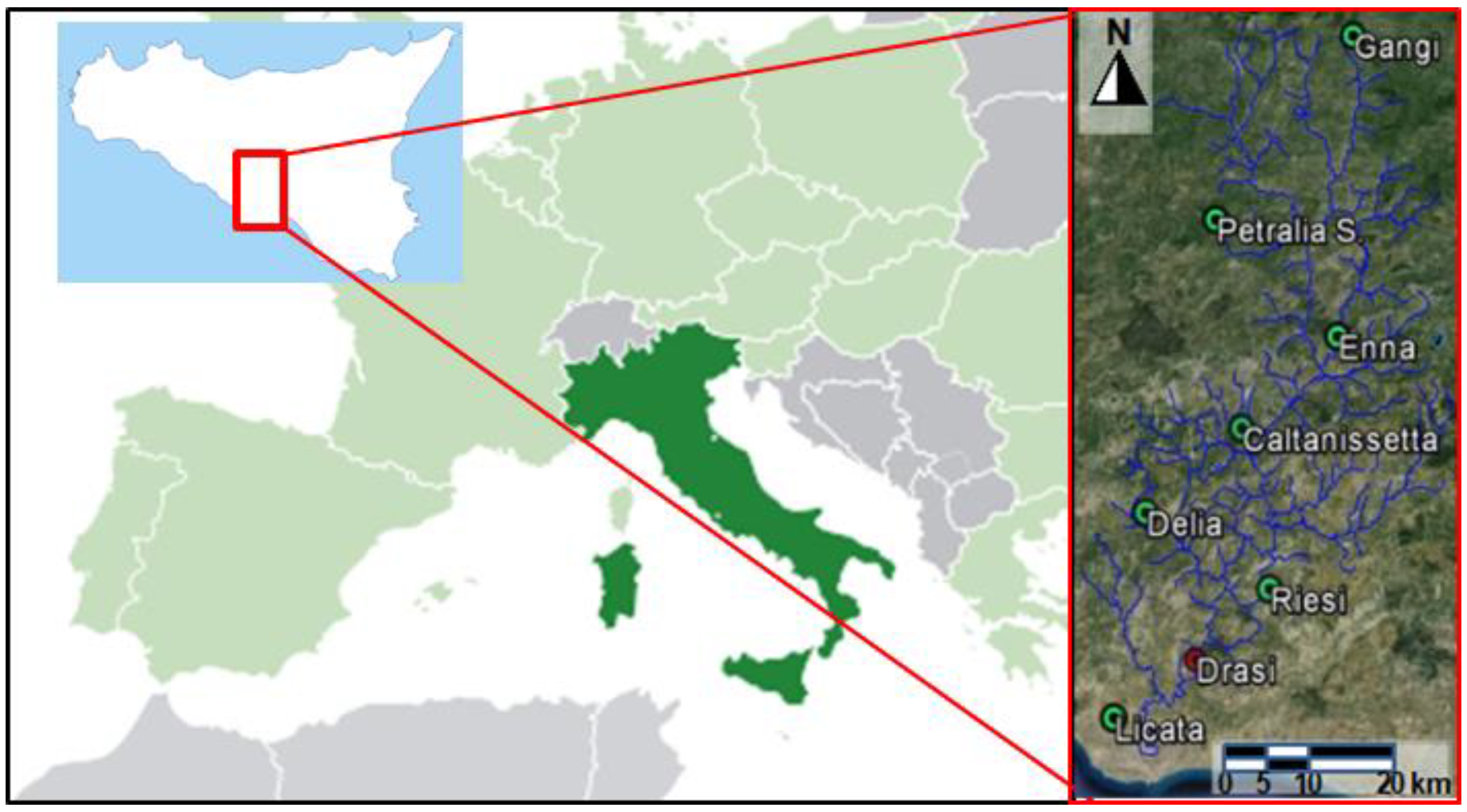
2.1. Study Area
2.2. Data
2.3. Methods
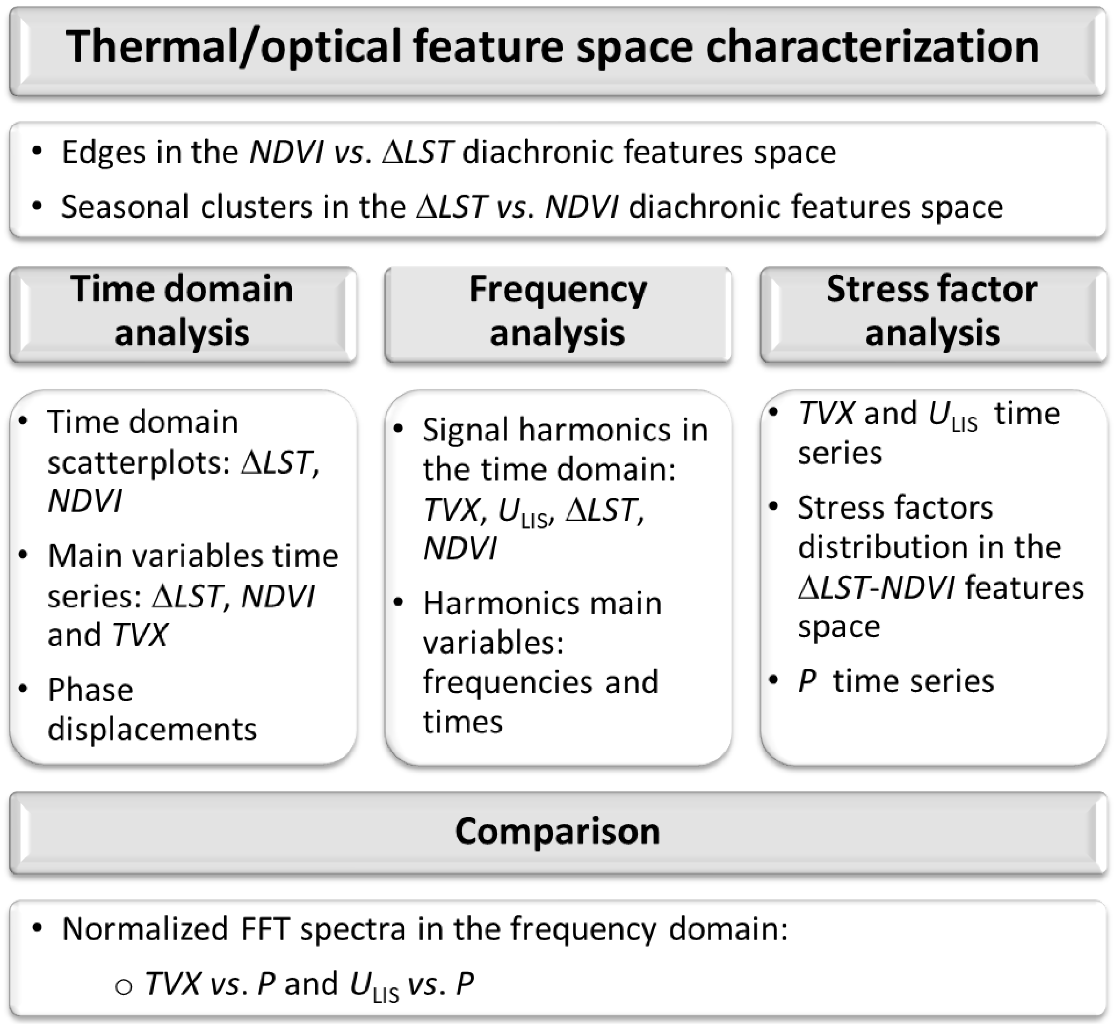
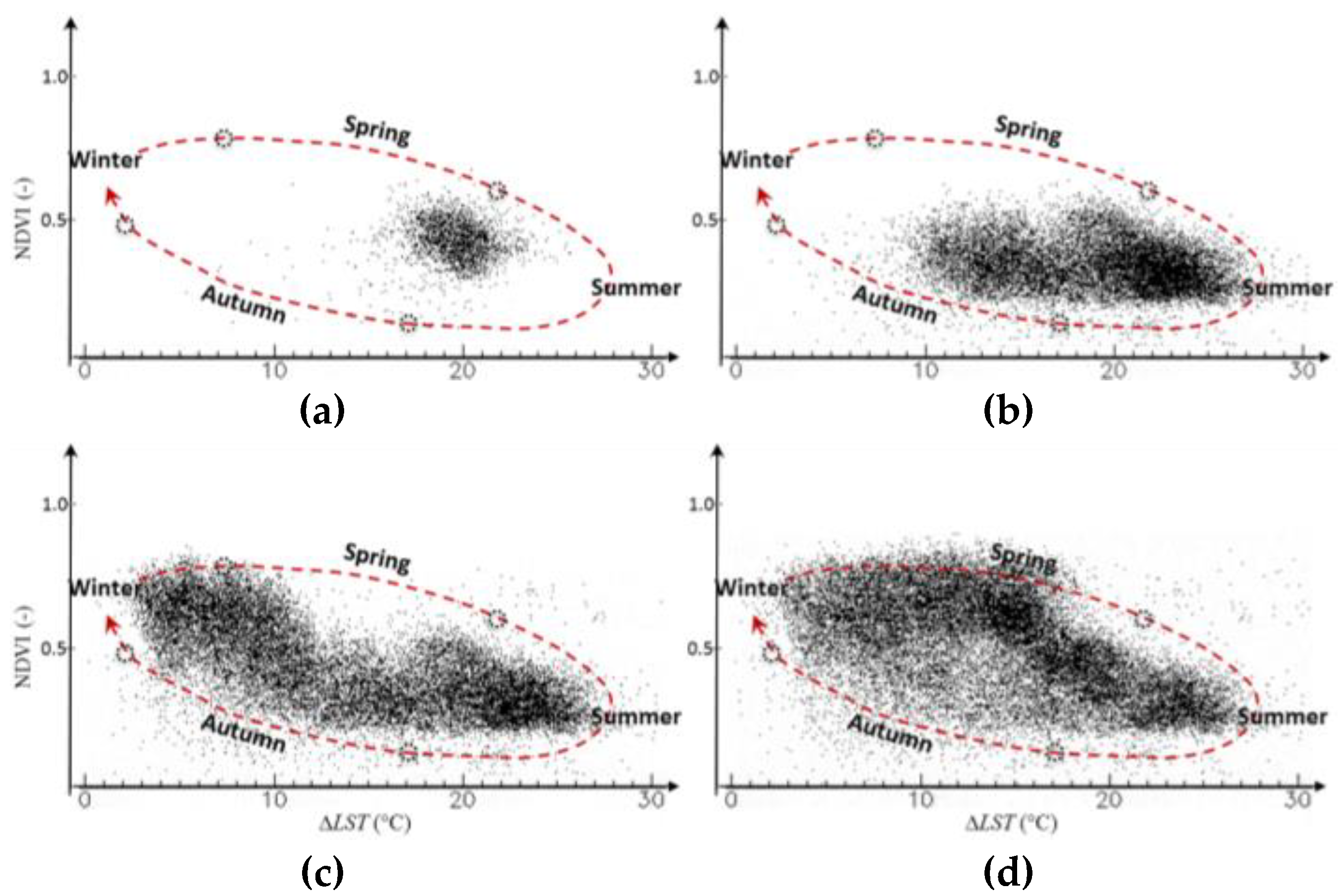
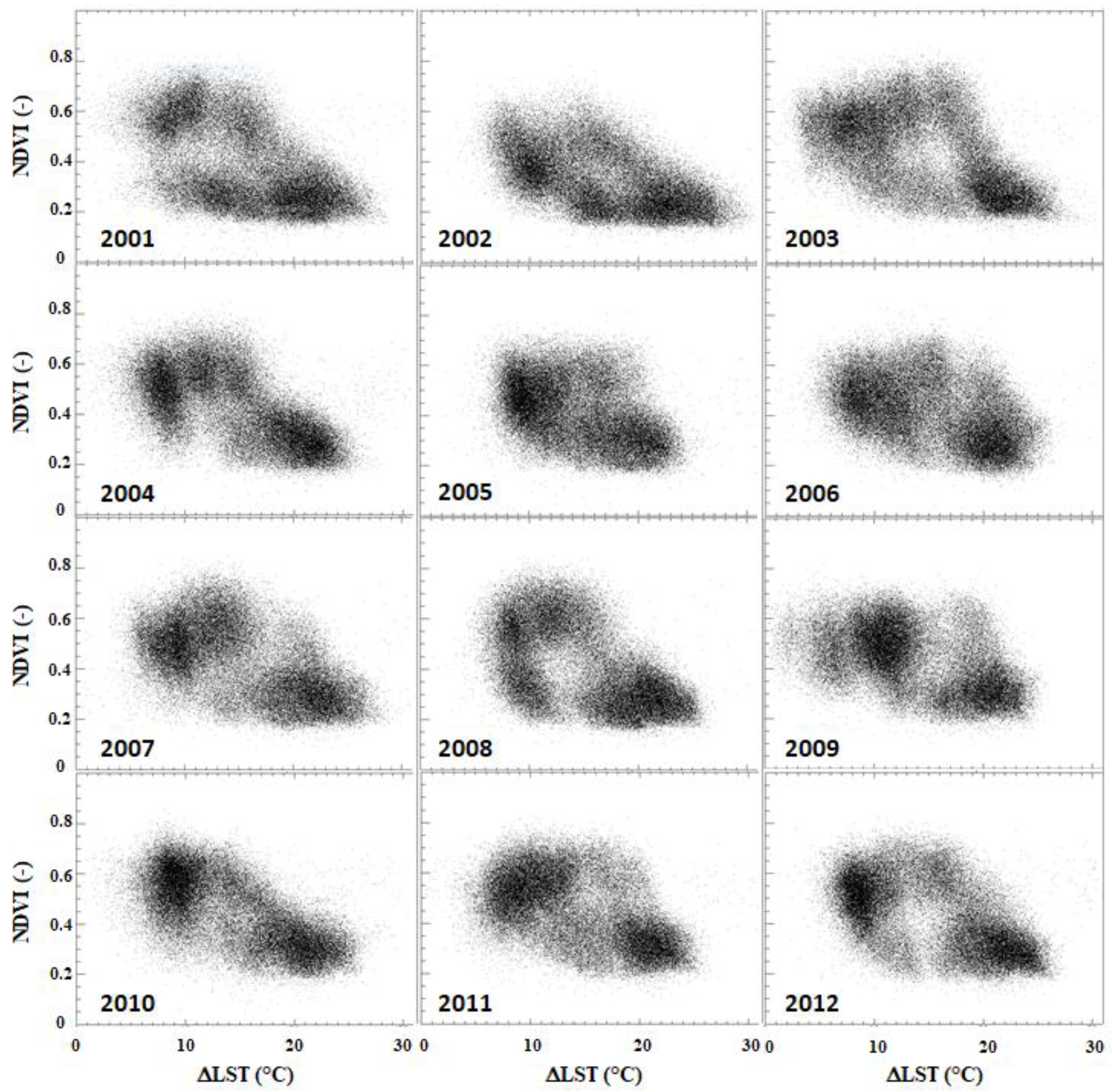
2.3.1. Thermal/Optical Features Space Characterization
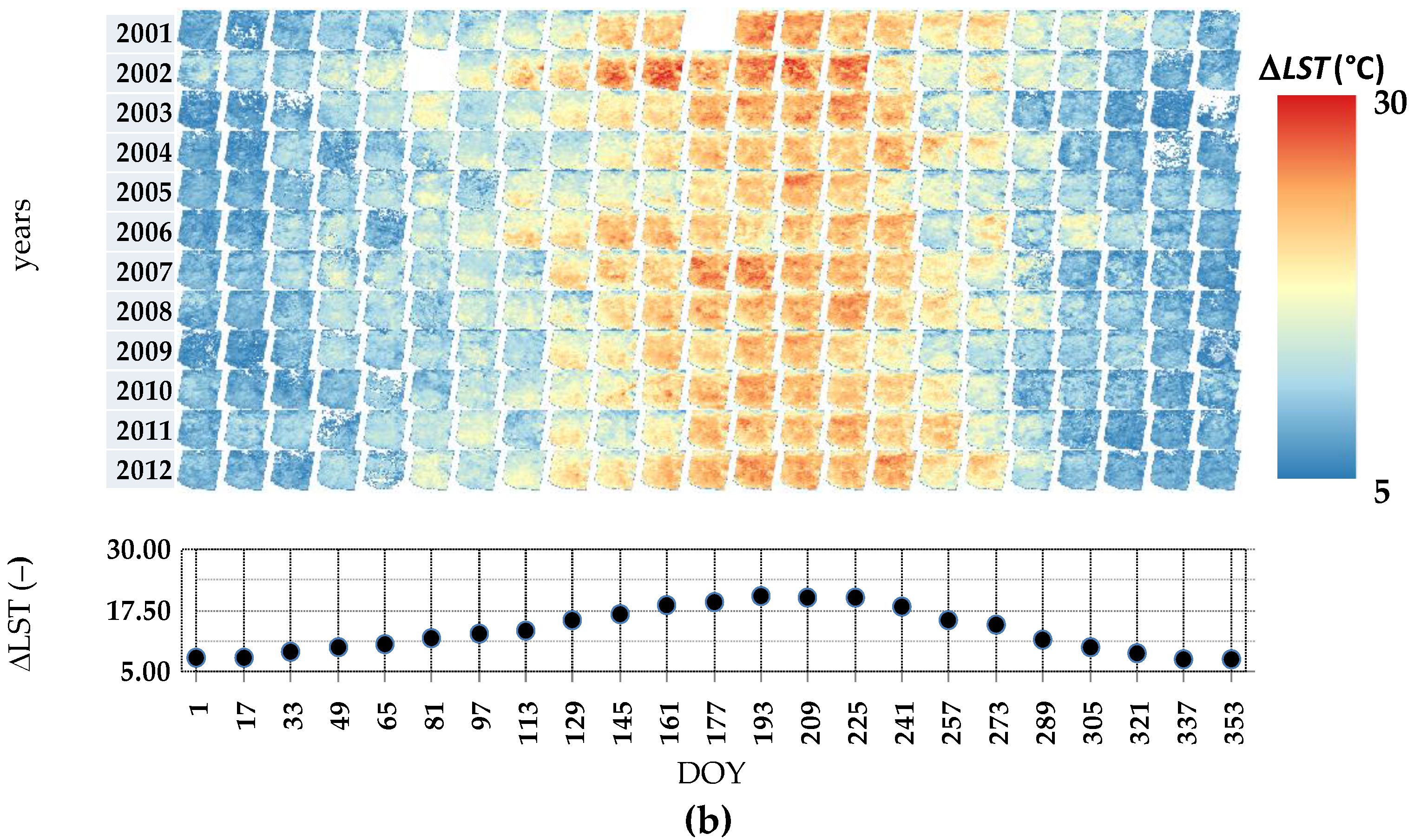
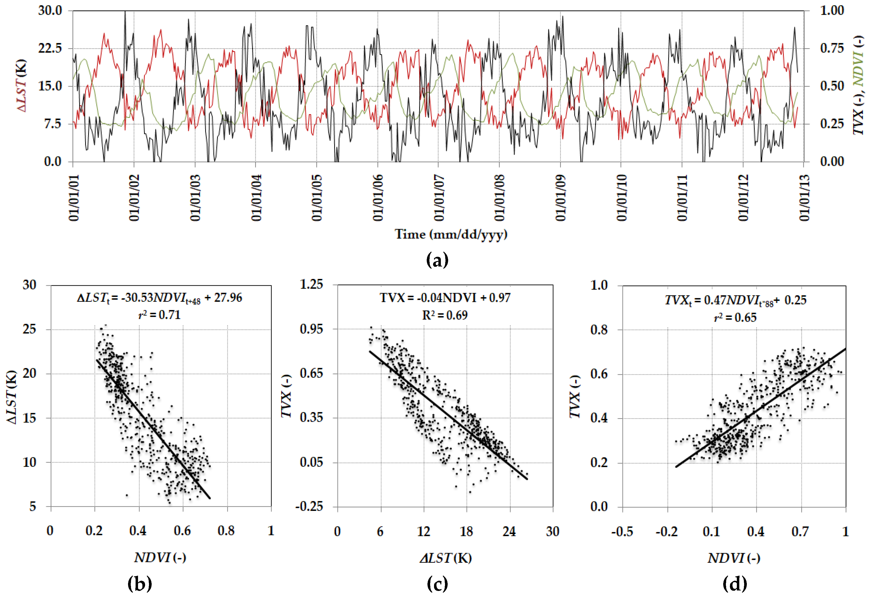
2.3.2. Time-Domain Analysis
2.3.3. Stress Factors Analysis
2.3.4. Frequency Domain Analysis
2.3.5. Comparisons
3. Results and Discussion
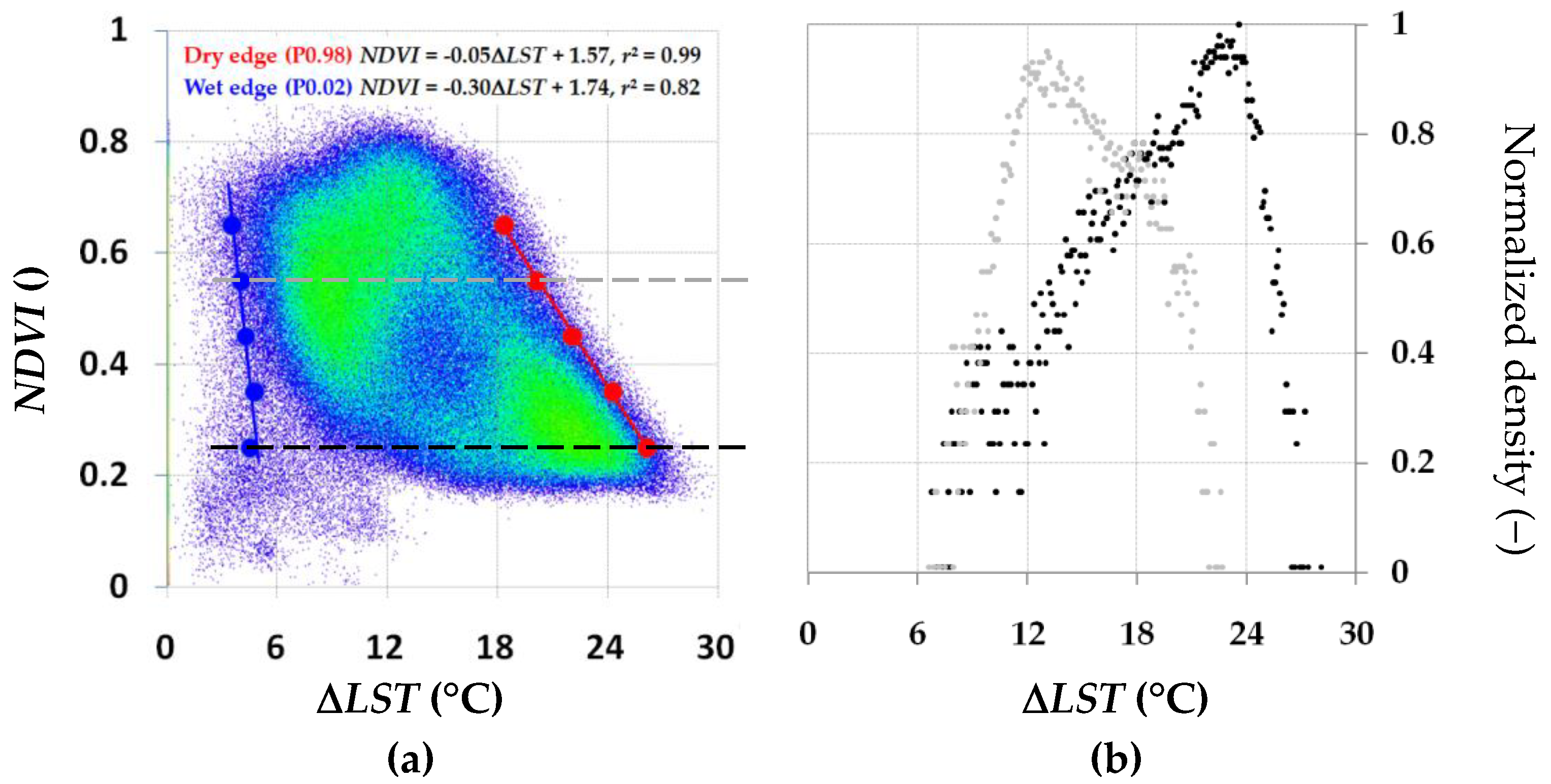
3.1. Thermal/Optical Features Space Characterization
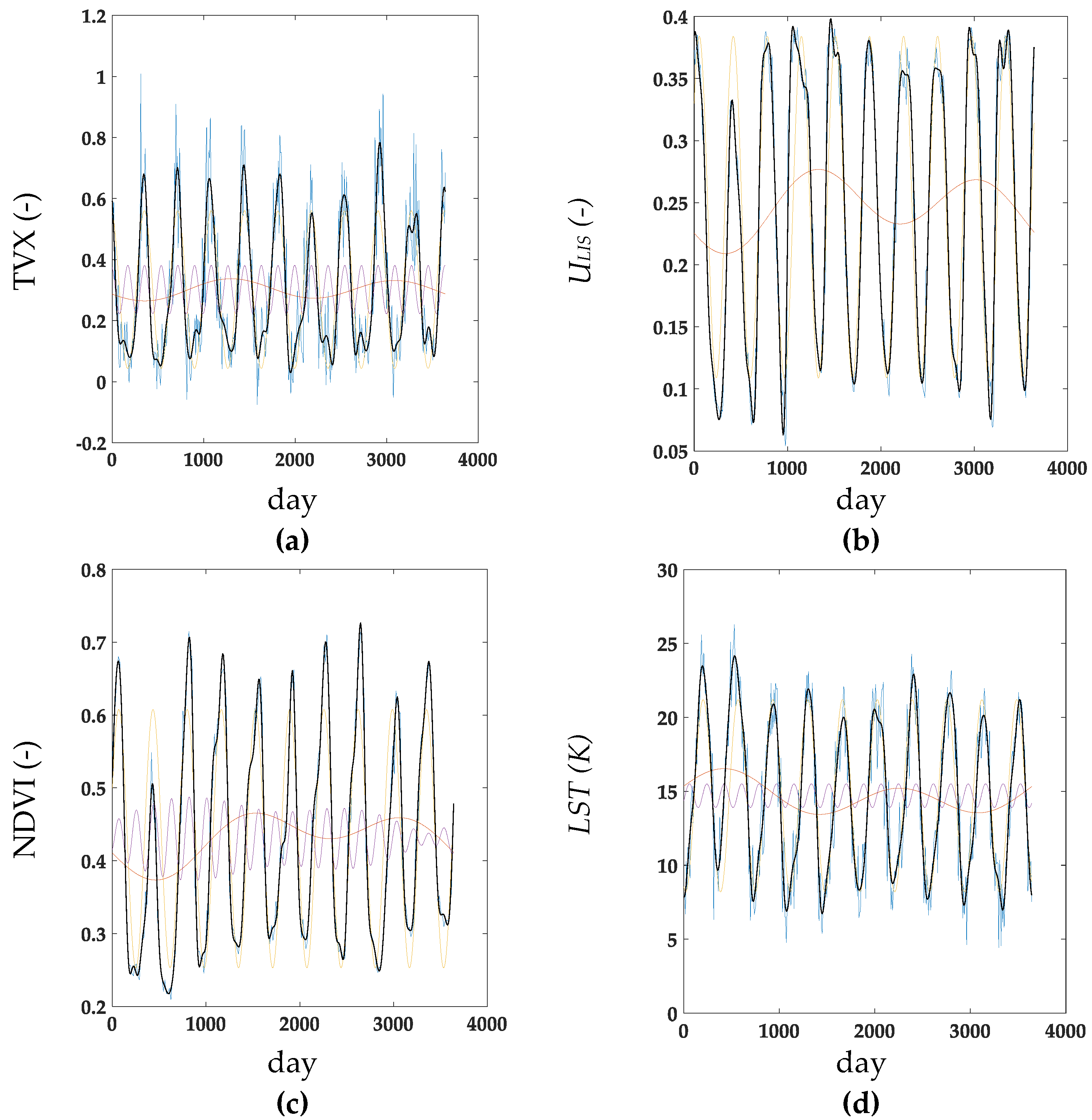
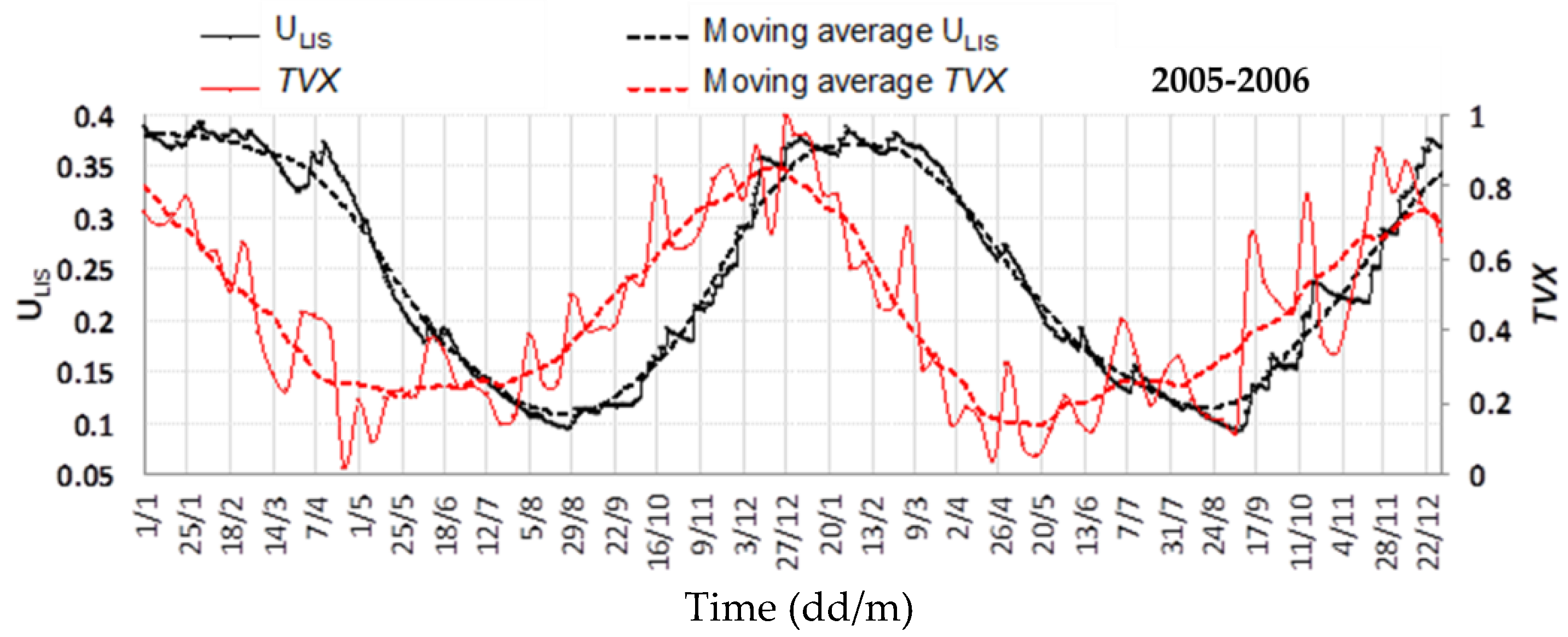
3.2. Time-Domain Analysis
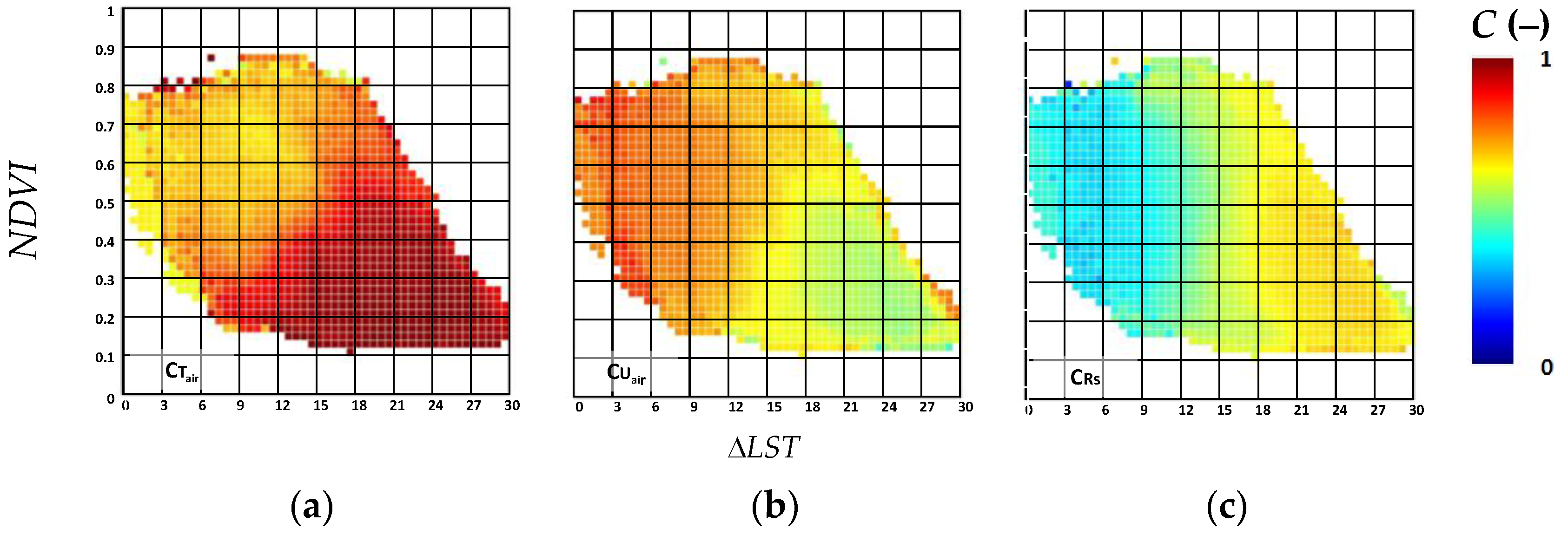
3.3. Stress Factor Analysis
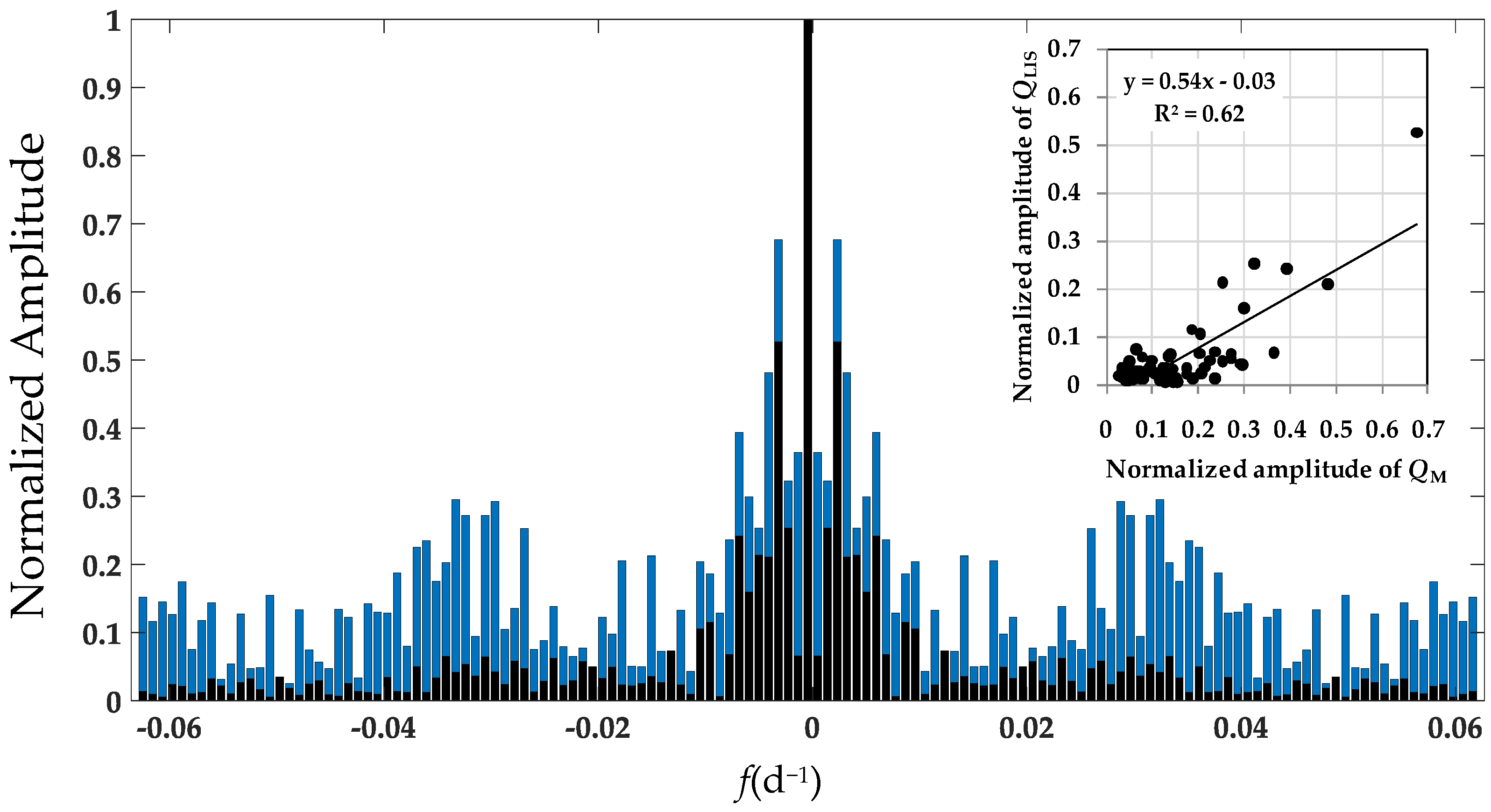
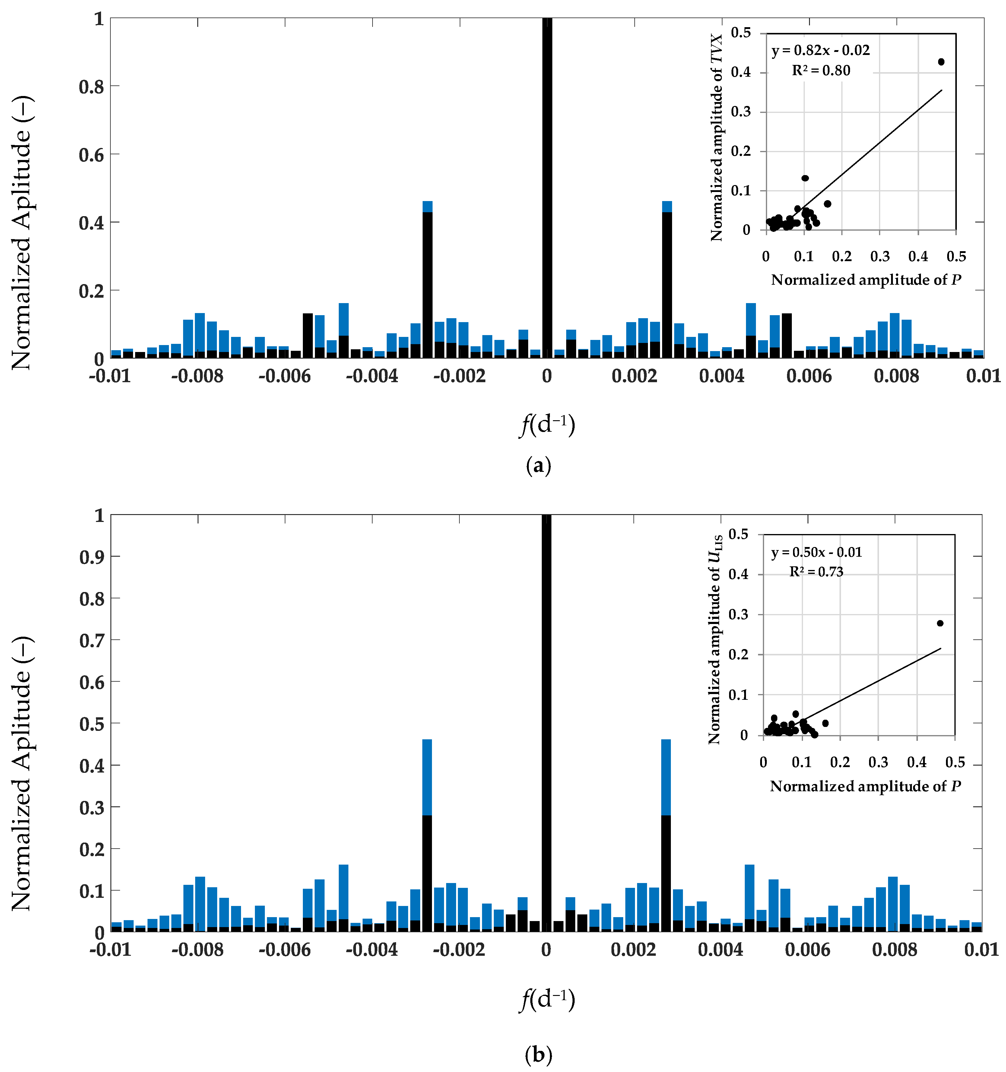
3.4. Frequency-Domain Analysis
4. Conclusions
Author Contributions
Funding
Acknowledgments
Conflicts of Interest
References
- Carlson, T.N.; Gillies, R.R.; Schmugge, T.J. An Interpretation of Methodologies for Indirect Measurement of Soil-Water Content. Agric. For. Meteorol. 1995, 77, 191–205. [Google Scholar] [CrossRef]
- Maltese, A.; Minacapilli, M.; Cammalleri, C.; Ciraolo, G.; D’Asaro, F. A thermal inertia model for soil water content retrieval using thermal and multispectral images. In Proceedings of the Remote Sensing for Agriculture, Ecosystems, and Hydrology XII, Toulouse, France, 20–23 September 2010; p. 78241G. [Google Scholar]
- Maltese, A.; Capodici, F.; Corbari, C.; Ciraolo, G.; La Loggia, G.; Sobrino, J.A. Critical analysis of the thermal inertia approach to map soil water content under sparse vegetation and changeable sky conditions. In Proceedings of the Remote Sensing for Agriculture, Ecosystems, and Hydrology XIV, Edinburgh, UK, 24–27 September 2012; p. 85310T. [Google Scholar]
- Maltese, A.; Capodici, F.; Ciraolo, G.; La Loggia, G. Soil Water Content Assessment: Critical Issues Concerning the Operational Application of the Triangle Method. Sensors 2015, 15, 6699–6718. [Google Scholar] [CrossRef] [PubMed]
- Wang, K.; Li, Z.; Cribb, M. Estimation of evaporative fraction from a combination of day and night land surface temperatures and NDVI: New method to determine the Pristeley-Taylor parameter. Remote Sens. Environ. 2006, 102, 293–305. [Google Scholar] [CrossRef]
- Minacapilli, M.; Consoli, S.; Vanella, D.; Ciraolo, G.; Motisi, A. A time domain triangle method approach to estimate actual evapotranspiration: Application in a Mediterranean region using MODIS and MSG-SEVIRI products. Remote Sens. Environ. 2016, 174, 10–23. [Google Scholar] [CrossRef]
- Stisen, S.; Sandholt, I.; Norgaard, A.; Fensholt, R.; Jensen, J.K. Combining the triangle method with thermal inertia to estimate regional evapotranspiration—Applied to MSG SEVIRI data in the Senegal River basin. Remote Sens. Environ. 2008, 112, 1242–1255. [Google Scholar] [CrossRef]
- Stisen, S.; Sandholt, I.; Nørgaard, A.; Fensholt, R.; Eklundh, L. Estimation of diurnal air temperature using MSG SEVIRI data in West Africa. Remote Sens. Environ. 2007, 110, 262–274. [Google Scholar] [CrossRef]
- Wang, S.; Garcia, M.; Ibrom, A.; Jakobsen, J.; Köppl, C.J.; Mallick, K.; Looms, M.C.; Bauer-Gottwein, P. Mapping root-zone soil moisture using a temperature-vegetation triangle approach with an unmanned aerial system: Incorporating surface roughness from structure from motion. Remote Sens. 2018, 10, 1978. [Google Scholar] [CrossRef] [Green Version]
- Goetz, S.J. Multi-sensor analysis of NDVI, surface temperature and biophysical variables at a mixed grassland site. Int. J. Remote Sens. 1997, 18, 71–94. [Google Scholar] [CrossRef]
- Sandholt, I.; Rasmussen, K.; Andersen, J. A simple interpretation of the surface temperature/vegetation index space for the assessment of surface moisture status. Remote Sens. Environ. 2002, 79, 213–224. [Google Scholar] [CrossRef]
- Shellito, P.J.; Small, E.E.; Colliander, A.; Bindlish, R.; Cosh, M.H.; Berg, A.A.; Bosch, D.D.; Caldwell, T.G.; Goodrich, D.C.; McNairn, H.; et al. SMAP soil moisture drying more rapid than observed in situ following rainfall events: Smap soil moisture drying. Geophys. Res. Lett. 2016, 43, 8068–8075. [Google Scholar] [CrossRef] [Green Version]
- Higuchi, A.; Hiyama, T.; Fukuta, Y.; Suzuki, R.; Fukushima, Y. The behaviour of a surface temperature/vegetation index (TVX) matrix derived from 10-day composite AVHRR images over monsoon Asia. Hydrol. Process. 2007, 21, 1157–1166. [Google Scholar] [CrossRef]
- LISFLOOD—Distributed Water Balance and Flood Simulation Model—Revised User Manual. 2013. Available online: https://ec.europa.eu/jrc/en/publication/eur-scientific-and-technical-research-reports/lisflood-distributed-water-balance-and-flood-simulation-model-revised-user-manual-2013 (accessed on 27 October 2019).
- Cammalleri, C.; Ciraolo, G.; La Loggia, G.; Maltese, A. Daily evapotranspiration assessment by means of residual surface energy balance modeling: A critical analysis under a wide range of water availability. J. Hydrol. 2012, 452–453, 119–129. [Google Scholar] [CrossRef]
- Cammalleri, C.; La Loggia, G.; Maltese, A. Critical analysis of empirical ground heat flux equations on a cereal field using micrometeorological data. In Proceedings of the Remote Sensing for Agriculture, Ecosystems, and Hydrology XI, Berlin, Germany, 1–3 September 2009; p. 747225. [Google Scholar]
- Scordo, A.; Maltese, A.; Ciraolo, G.; La Loggia, G. Estimation of the time lag occurring between vegetation indices and aridity indices in a Sicilian semi-arid catchment. Ital. J. Remote Sens. 2009, 41, 33–46. [Google Scholar] [CrossRef]
- Péguy, C.P. Une tentative de délimitation et de schématisation des climats intertropicaux. Rev. Geogr. 1961, 36, 1–6. [Google Scholar] [CrossRef]
- Osservatorio Delle Acque, Servizio Osservatorio delle Acque del Dipartimento dell’Acqua e dei Rifiuti, Assessorato Regionale dell’Energia e dei servizi di Pubblica Utilità, Regione Siciliana, Stazione idrografica di Imera Meridionale a Drasi. Available online: http://www.a3studio.it/meteo/datistazione.php?id=105 (accessed on 27 October 2019).
- Servizio Informativo Agrometeorologico Siciliano (SIAS). Available online: http://www.sias.regione.sicilia.it/ (accessed on 27 October 2019).
- Testa, S.; Mondino, E.C.; Pedroli, C. Correcting MODIS 16-day composite NDVI time-series with actual acquisition dates Correcting MODIS 16-day composite. Eur. J. Remote Sens. 2014, 47, 285–305. [Google Scholar] [CrossRef]
- Thielen, J.; Bartholmes, J.; Ramos, M.H.; de Roo, A. The European Flood Alert System—Part 1: Concept and development. Hydrol. Earth Syst. Sci. 2009, 13, 125–140. [Google Scholar] [CrossRef] [Green Version]
- Alfieri, L.; Salamon, P.; Bianchi, A.; Neal, J.; Bates, P.; Feyen, L. Advances in pan—European flood hazard mapping. Hydrol. Process. 2014, 28, 4067–4077. [Google Scholar] [CrossRef]
- Cammalleri, C.; Micale, F.; Vogt, J. On the value of combining different modelled soil moisture products for European drought monitoring. J. Hydrol. 2015, 525, 547–558. [Google Scholar] [CrossRef]
- Laguardia, G.; Niemeyer, S. On the comparison between the LISFLOOD modelled and the ERS/SCAT derived soil moisture estimates. Hydrol. Earth Syst. Sci. 2008, 12, 1339–1351. [Google Scholar] [CrossRef] [Green Version]
- Carlson, T. An overview of the “triangle method” for estimating surface evapotranspiration and soil moisture from satellite imagery. Sensors 2007, 7, 1612–1629. [Google Scholar] [CrossRef] [Green Version]
- Jarvis, P.G. The interpretation of leaf water potential and stomatal conductance found in canopies in the field. Philos. Trans. R. Soc. London B Biol. Sci. 1976, 273, 593–610. [Google Scholar] [CrossRef]
- Noilhan, J.; Planton, S. A simple parameterization of land surface processes for meteorological models. Mon. Weather Rev. 1989, 117, 536–549. [Google Scholar] [CrossRef]
- Goward, S.N.; Xue, Y.; Czajkowski, K.P. Evaluating land surface moisture conditions from the remotely sensed temperature/vegetation index measurements: An exploration with the simplified simple biosphere model. Remote Sens. Environ. 2002, 79, 225–242. [Google Scholar] [CrossRef]
- Prino, S.; Spanna, F.; Cassardo, C. Verification of the stomatal conductance of Nebbiolo grapevine. J. Chongqing Univ. 2009, 1, 1724. [Google Scholar]
- Sepulveda, G.; Kliewer, W.M. Stomatal response of three grapevine cultivars (Vitis vinifera L.) to high temperature. Am. Soc. Enol. Vitic. 1986, 37, 44–52. [Google Scholar]
- Stewart, J.B.; Gay, L.W. Preliminary modelling of transpiration from the FIFE site in Kansas. Agric. For. Meteorol. 1989, 48, 305–315. [Google Scholar] [CrossRef]
- Cramer, M.D.; Hoffmann, V.; Verboom, G.A. Nutrient availability moderates transpiration in Ehrharta calycina. New Phytol. 2008, 179, 1048–1057. [Google Scholar] [CrossRef]
- Evans, J.D. Straightforward Statistics for the Behavioral Sciences; Brooks/Cole Publishing: Pacific Grove, CA, USA, 1996. [Google Scholar]
- Schatzman, J.C. Accuracy of the discrete Fourier transform and the fast Fourier transform. SIAM J. Sci. Comput. 1996, 17, 1150–1166. [Google Scholar] [CrossRef] [Green Version]
- Cooley, J.W.; Tukey, J.W. An algorithm for the machine calculation of complex Fourier series. Math. Comput. 1965, 19, 297–301. [Google Scholar] [CrossRef]
- Brockwell, P.J.; Davis, R.A. Introduction to Time-Series and Forecasting; Springer International Publishing: Cham, Switzerland, 2016. [Google Scholar]
- Mathworks. Available online: https://www.mathworks.com/help/matlab/math/fourier-transforms.html?searchHighlight=fftshift&s_tid=doc_srchtitle (accessed on 27 October 2019).
- Zhang, R.; Tian, J.; Su, H.; Sun, X.; Chen, S.; Xia, J. Two improvements of an operational two-layer model for terrestrial surface heat flux retrieval. Sensors 2008, 8, 6165–6187. [Google Scholar] [CrossRef]


| Variable(s) | Harmonic | Peak Frequency (d−1 × 10⁻³) | Band-Pass Range (d−1 × 10⁻³) | Periodicity (d) | Peak Time (DOY) |
|---|---|---|---|---|---|
| ULIS | 0 | 0–0.6 | 1700 | 1337/3041 | |
| 1 | 2.737 | 2.50–3.00 | 365 | 57 | |
| TVX | 0 | 0–0.6 | 1800 | 1305/3105 | |
| 1 | 2.737 | 2.50–3.00 | 365 | 348 | |
| 2 | 5.457 | 5.25–5.70 | 182 | 168/350 | |
| ΔLST | 0 | 0–0.6 | 1630 | 1433/3065 | |
| 1 | 2.737 | 2.50–3.00 | 365 | 200 | |
| 2 | 5.457 | 5.25–5.70 | 182 | 60/240 | |
| NDVI | 0 | 0–0.6 | 1528 | 1537/3065 | |
| 1 | 2.737 | 2.50–3.00 | 365 | 70 | |
| 2 | 5.457 | 4.80–5.70 | 182 | 70/250 |
© 2020 by the authors. Licensee MDPI, Basel, Switzerland. This article is an open access article distributed under the terms and conditions of the Creative Commons Attribution (CC BY) license (http://creativecommons.org/licenses/by/4.0/).
Share and Cite
Capodici, F.; Cammalleri, C.; Francipane, A.; Ciraolo, G.; La Loggia, G.; Maltese, A. Soil Water Content Diachronic Mapping: An FFT Frequency Analysis of a Temperature–Vegetation Index. Geosciences 2020, 10, 23. https://doi.org/10.3390/geosciences10010023
Capodici F, Cammalleri C, Francipane A, Ciraolo G, La Loggia G, Maltese A. Soil Water Content Diachronic Mapping: An FFT Frequency Analysis of a Temperature–Vegetation Index. Geosciences. 2020; 10(1):23. https://doi.org/10.3390/geosciences10010023
Chicago/Turabian StyleCapodici, Fulvio, Carmelo Cammalleri, Antonio Francipane, Giuseppe Ciraolo, Goffredo La Loggia, and Antonino Maltese. 2020. "Soil Water Content Diachronic Mapping: An FFT Frequency Analysis of a Temperature–Vegetation Index" Geosciences 10, no. 1: 23. https://doi.org/10.3390/geosciences10010023