Biosignatures Search in Habitable Planets


1
INAF-Astronomical Observatory of Padova, Vicolo Osservatorio, 5, 35122 Padova, Italy
2
Physics and Astronomy Department, Padova University, 35131 Padova, Italy
*
Author to whom correspondence should be addressed.
Galaxies 2019, 7(4), 82; https://doi.org/10.3390/galaxies7040082
Submission received: 2 August 2019
/
Revised: 20 September 2019
/
Accepted: 25 September 2019
/
Published: 29 September 2019
(This article belongs to the Special Issue Habitability of Planets in Stellar Binary Systems)
Abstract
:The search for life has had a new enthusiastic restart in the last two decades thanks to the large number of new worlds discovered. The about 4100 exoplanets found so far, show a large diversity of planets, from hot giants to rocky planets orbiting small and cold stars. Most of them are very different from those of the Solar System and one of the striking case is that of the super-Earths, rocky planets with masses ranging between 1 and 10 M with dimensions up to twice those of Earth. In the right environment, these planets could be the cradle of alien life that could modify the chemical composition of their atmospheres. So, the search for life signatures requires as the first step the knowledge of planet atmospheres, the main objective of future exoplanetary space explorations. Indeed, the quest for the determination of the chemical composition of those planetary atmospheres rises also more general interest than that given by the mere directory of the atmospheric compounds. It opens out to the more general speculation on what such detection might tell us about the presence of life on those planets. As, for now, we have only one example of life in the universe, we are bound to study terrestrial organisms to assess possibilities of life on other planets and guide our search for possible extinct or extant life on other planetary bodies. In this review, we try to answer the three questions that also in this special search, mark the beginning of every research: what? where? how?
1. Introduction
Since the ancient times, philosophers try to answer to the question “are we alone?” Up to now no certain answer has been given due mainly to the huge technological challenge in unveiling extant life (if any) on alien worlds. Giuseppe Conconi and Phillip Morrison in their seminal paper [1] exhorted scientists to be engaged in any case in this quest with their famous sentence: the probability of success is difficult to estimate, but if never search the chance of success is zero. Just after, the SETI (Search for Extraterrestrial Intelligence) project started ([2] and see [3] for a review) together with its expectations and eerie silences [4].
The search for life in the Galaxy received a big boost by the bonanza of new worlds discovered so far, also if we are compelled to tackle with the distances at which these worlds are. In fact, it is quite different for searching life in the Solar System bodies where, also if with great technological efforts and challenges, it is possible to explore them on-site and investigate if they are bearing life. Venus and Mars are targets of this wandering of the human beings in the Solar System. In the case of extrasolar planets, the only way to search for life is the remote sensing.
So, one of the big questions on the mat is what we are searching for? A really hard question. Life, as we know it, has been described as a (thermodynamically) open system [5], which exploits gradients in its surroundings to create imperfect copies of itself, makes use of chemistry based on carbon, and exploits liquid water as solvent for the necessary chemical reactions [6,7]. This seems an a priori and quite geocentric statement, but considering life as a stochastic process, it has a non–zero probability of occurring as soon as the environmental conditions for its appearance are met. If this is the case, we have to consider all the circumstances that can maximize this probability. In this framework, the carbon is the only chemical element with which it is possible to form very complex molecules with up to 13 atoms (e.g., HCN). Carbon is also very easy to reduce (CH) and oxidize (CO).
On the other hand, liquid water has some important characteristics that make it the best solvent for life: a large dipole moment, the capability to form hydrogen bonds, to stabilize macromolecules, to orient hydro–phobic–hydrophilic molecules, etc. Furthermore, water is an abundant compound in our galaxy, that is possible to find in different environments, like cold dense molecular clouds and hot stellar atmospheres, e.g., [8,9]. Water is liquid at a large range of temperatures and pressures and it is a strong polar—non polar solvent. This dichotomy is essential for maintaining stable biomolecular and cellular structures [7]. Furthermore, liquid water has a great heat capacity that makes it able to tolerate a heat shock. The most common solid form of water has a specific weight lighter than that of its liquid form allowing ice to float on a liquid ocean safeguarding the underlying liquid water. All those characteristics let grow the probability that life, once it emerges, could survive and evolve.
For all these reasons, we will base our search for signs of life (biosignatures) on the assumption that alien life shares fundamental characteristics with life on Earth. Life based on a different chemistry is not considered here because such life—forms, should they exist, would have by–products that are so far unknown.
The word “Biosignature” identifies all detectable atmospheric gas species, or a set of species, whose presence at significant abundance strongly suggests a biological origin [7]. Instead the term bioindicators defines all the other gases that are or could be indicative of biological processes but can also be produced abiotically (e.g., on Earth, O is the photochemical by-product of O). Their quantity and detection, along with other atmospheric species, all within a certain context (for instance, the properties of the star and the planet) points toward a biological origin. These gases should be ubiquitous by-products of carbon-based biochemistry, even if the details of alien biochemistry are significantly different from the biochemistry on Earth. Besides atmospheric biosignatures, there are also life signatures due to the light reflection characteristics of specific components of living being as, for example pigments, that can modify or contribute to the planetray albedo. These are called surface biosignatures and are also detectable by remote sensing, e.g., [10].
The debate about biosignatures and remote sensing search for life is growing livelily in the last years and several reviews tackle the topic [7,10,11,12,13,14,15,16,17,18,19,20,21,22,23,24] and references therein, where the reader can find precise information on this topic. In this paper the main results of these authors will be summarized.
Atmospheric biosignatures, bioindicators and surface and industrial biosignatures are described from Section 2 to Section 4 while in Section 5 a description of the possible false positives is given. Section 6 introduces the concept of the habitable zone. The detection methods are discussed in Section 7 and the perspective for the future are outlined in Section 8. Finally, in Section 9 we give a summary and outline the conclusions.
2. Atmospheric Biosignatures
The approach to remote detection of signs of life on another planet was set out in the last century by Lederberg [25] and Lovelock [26], which introduced the concept for the search for an atmosphere containing gases severely out of thermochemical redox equilibrium1 like for example the simultaneous presence of O and CH [27]. The idea that gas by–products from metabolic redox reactions can accumulate in the atmosphere was initially favoured for future sign of life identification, because abiotic processes were thought to be less likely to create a redox disequilibrium.
Lippincot and collaborators [27] found that on Earth other than CH there are also other gases (H, NO, and SO) out of thermodynamic equilibrium, but they all (with the possible exception of NO) are also by-product of geochemical processes and cannot be considered unambiguous signs of life.
In a meeting held in the 1975, Lovelock et al. [28] supported the idea of Lippincott et al. [27] that the O–CH disequilibrium was strong evidence for life, and from then on, CH was established as a biosignature gas [28,29]. This is an appealing concept because the chemical disequilibrium could be considered a generalized biosignature and it is not necessary to have any assumption on particular biogenic and metabolic by–product gas. This concept has been explored also in the recent years [30,31,32], but no additional, potentially observable disequilibrium redox pair has been identified (but see ahead).
In any case, many reasons suggest to use with prudence the thermodynamic disequilibrium as a life indicator [33]. First of all almost any gas, in Earth’s atmosphere, other than N and CO, is out of thermodynamic equilibrium because of the Earth’s high O level. So, the argument that Earth’s atmosphere is out of thermodynamic equilibrium reduces to a statement about the high levels of Earth’s atmospheric O. Even if no or too few O is present, it is possible to have a significant thermodynamic disequilibrium due to geochemical or photochemical processes. On the other hand, Krissansen-Totton and collaborators [19] in their study on the atmosphere-ocean disequilibrium in the precambrian, found that in different era there should be different disequilibrium stages due to the coexistence of O, N and also N, CH, CO and liquid water that could be remotely detected. They concluded that the simultaneous detection of CH and CO in the atmosphere of an habitable planet could be a potential biosignature.
The chemicals produced by life on Earth are hundreds of thousands [16] (estimated from plant natural products, microbial natural products, and marine natural products), but only a subset of hundreds are volatile enough to enter the atmosphere at more than trace concentrations. Among these, only a few handfuls accumulate to high enough levels to be remotely detectable for astronomical purposes and defined as biosignatures. Apart from oxygen, these biosignature (and bioindicator) gases range from highly abundant gases in Earth’s atmosphere that are either already existing or predominantly produced by geochemical or photochemical processes (N, Ar, CO, and HO) to those that are relatively abundant and attributed to life (NO, CH and HS). We have to consider also gases that are weakly present but may play important roles in the atmospheric processes (DMDS and CHCl) and gases that are present only in trace amounts including the hundreds of minutely present volatile organic compounds released by trees in a forest or fungi in the soil [16].
The first remote observation of biosignatures could be considered the UV, visible and NIR spectra of the Earth obtained by the probe Galileo in its fly towards Jupiter in the 1990. Sagan et al. [34] analyzed those spectra searching for signatures of life. In the spectra of the Near–Infrared Mapping Spectrometer (NIMS, [35]) they found a large amount of O and the simultaneous presence of CH traces concluding that this co–presence is strongly suggestive of life (see Figure 1).
Other observations of Earth as an exoplanet have performed in the last years observing the earthshine, the faint light seen on the dark side of crescent moon [36,37,38,39,40]. Earthshine is the Sun’s light reflected by the day-side of the Earth towards the dark side of the Moon and reflected again onto the night side of the Earth where it is caught by ground-based telescopes. In the earthshine spectra it is possible to observe prominent oxygen absorption feature at 0.76 m, instead methane has only extremely weak spectral features (at present day the levels is 1.6 ppm). Furthermore, on Earth, some atmospheric species that show observable spectral features come directly or indirectly from biological activity. The main molecules are O, O, CH, and NO. Both CO and HO are important greenhouse gases and also potential sources for high O concentration from photosynthesis. Furthermore, the earthshine has been analyzed by a polarimetric point of view. When light passes through the atmosphere, it is linearly polarized by air molecules, aerosol and cloud particles scattering. Reflection by ocean and land can also contribute to the linear polarization of light [41]. Sterzik et al. [42], using FORS (Focal Reducer Low-dispersion Spectrograph [43]) at VLT, measured the linear polarization spectra of the earthshine, determining the fractional contribution of clouds and ocean surface.
In order to describe the possible biosignature gases that are possible to detect by remote sensing, we have to take into account the by–products of the following processes: (i) the metabolic chemical reactions; (ii) the chemical reaction for the construction of organic matter, (iii) the secondary metabolic chemical reactions.
2.1. Metabolic Biosignatures
This biosignatures category contents all those by–product gases due to metabolic reactions that capture energy from environmental redox chemical potential energy gradients [12,13]. Such gases (see Table 1 for aerobic chemotrophy and Table 2 for anaerobic chemotrophy) are abundant due to the presence of large quantity of reactants in the environment, but they could not be considered as produced exclusively by life. In fact, geology for example, works on the same molecules as life does. Moreover, in one environment, a given redox reaction will be kinetically inhibited and it is only started by life’s enzymes, while in another environment with the right conditions (temperature, pressure, concentration and acidity), the same reaction might proceed spontaneously.
An interesting biosignature of this category is Nitrous oxide (NO [24,34,44,45,46,47,48]). It is produced in abundance by life (denitrifying bacteria) but only in negligible amounts by abiotic processes. Most of the reaction that produce NO are listed in Table 2, a simple scheme of the denitrification reaction is the following:
It is difficult to be detected, especially in a humid atmosphere where the molecular band of water vapour, CO and CH are generally overimposed to the NO features. It would become more apparent in atmospheres with more NO or less HO vapor, or a combination of the two [49]. Segura et al. [50] calculated the level of NO for different O levels and found that, though NO is a reduced species compared to N, its level decreases with O. This is due to the fact that a decrease in O produces an increase in HO photolysis, which results in the production of more hydroxyl radicals (OH) responsible for the destruction of NO. In the near–UV and blue optical region, NO and NO have molecular transition bands, but their strength is smaller, in a significant way, than those of other molecules, like O and O, that are in the same spectral region. Other features of NO are present in the IR wavelength range (m and m), but also in this case they are pretty weak features and difficult to be detected [24,45].
Abiotic sources of NO are small and are due mainly to the chemodenitrification process, like that occurs in the hypersaline ponds in Antartica [22,51] and, depending by the redox state of the environment, to the high temperature reduction and oxidation reactions of N. These reactions occur for combustion or lightings transforming the resulting molecules from N redox reactions (NH, HCN and NO) in water soluble molecules (e.g., HNO, [24]).
N is another metabolic product of denitrification, released when, under anaerobic environments, bacteria use oxygen by NO to convert carbon in CO. Anammox (anaerobic ammonium oxidation) is another anaerobic biological process that is the oxidation of NH with NO that produce N and HO (see Table 2 for other examples). This process can produce about 50% of the N produced in the ocean and that then is released in the atmosphere ([24], and references therein).
The production of methane by methanogen bacteria (methanogenesis) is a typical reaction of this category:
It is generated by bacteria at the sea floor which reduce the CO available in the sea water due to the mixing with the atmosphere using the H released by hot water coming from rocks (serpentinization). Most of the methane found in the present atmosphere of Earth has this biological origin, but methane is also produced abiotically in hydrothermal systems where hydrogen is released by the oxidation of Fe by HO and reacts with CO to form CH. The amount of CH produced in this process depends by the oxidation degree of the planetary crust. Therefore, the detection of CH alone cannot be considered as a sign of life, though its detection in an oxygen–rich atmosphere could be an indication of the presence of a biosphere.
On early Earth, CH might have been produced by widespread methanogen bacteria [52] at much higher levels (1000 ppm or even 1%). Such high CH concentrations would be easier to detect. On the other hand, at that time the contents of oxygen in the early Earth’s atmosphere was very small or even insignificant, the O–CH redox pairs would be difficult to be detected at present concurrently [7,53], unless perhaps in the case of a planet in a lower-UV (200–300 nm) radiation environment (possible with some M host stars [44]). The recent confirmation of methane in the atmosphere of Mars [54,55], that contains 0.1% of O and some O, is a good example for both the consideration of CH as a biosignature gas, since it is photochemically unstable and must be actively produced, but it is also an example for a false positive because CH could be produced geologically.
NH (a very similar case to the one of CH) is produced on Earth quite only by biological processes (anammox), apart from the one industrially manufactured. Both (NH and CH) are released into the Earth’s atmosphere by the biosphere with similar rates, but the atmospheric level of NH is orders of magnitude lower due to its very short lifetime under UV irradiation. The detection of NH in the atmosphere of a habitable planet would thus be extremely interesting, especially if found with oxidized species [49].
2.2. Organic Matter Building By–Products
This class of biomass building by-products records few biosignature gases (see Table 3) among its elements. These reactions require mainly energy from the environment and capture environmental carbon (and to a lesser extent other elements). The main example on Earth is O produced by oxygenic photosynthesis, which gains energy from sunlight. In more detail, photosynthesis captures the carbon in CO into biomass, releasing oxygen that, nowadays, is the 20% by volume of the Earth’s atmosphere. Less than 1 ppm of atmospheric O comes from abiotic processes [56]. This high quantity of such a reactive gas like O with a short atmospheric lifetime allows to consider oxygen a robust biosignature [57]. Owen [6] suggested searching for O as a tracer of life. In fact, without continual replenishment by photosynthesis in plants and bacteria, O would be ten orders of magnitude less than present today in the Earth’s atmosphere [58]. Any observer seeing oxygen in Earth’s spectrum would know that some non-geological chemistry must be producing it. At this point a warning should be raised. In fact, an important pathway for the formation of abiotic oxygen in an observable quantity is through the HO photodissociation by the EUV flux of the host star (see Section 5), followed by the Hydrogen escape from the gravitational pull of the planet [59,60,61].
Photosynthesis converts light energy to electrochemical energy by redox reactions. Light, exciting pigments, causes a transfer of electrons along bio–chemical pathways having as result the CO reduction. The electron is replaced by one extracted from the reductant. The basic stoichiometry of photosynthesis is [62]:
This is a general way to show the reaction for both oxygenic and anoxygenic photosynthesis. HX represents the reductant that could be HO (oxygenic photosynthesis) or HS (an-oxygenic photosynthesis), h is the photon energy (h is the Planck’s constant). In the case of oxygenic photosynthesis the reductant is water and we have the following reactions:
Because the two processes, light capture and biomass building, are mechanistically distinct, the complete reaction is split in two parts. The former reaction generates the electrons, while the latter synthesises carbohydrate (CHO). For each O molecule four photons are required (one photon for each bond in two water molecules) while other four photons are necessary to reduce CO. Thus, a minimum of eight photons is required both to evolve one O and to fix carbon from one CO.
Cyanobacteria, plants and algae are responsible for the production of oxygen by using solar photons to extract hydrogen from water (that is abundant on Earth) and using it to produce organic molecules from CO. The reverse reaction, using O to oxidize the organics produced by photosynthesis, can occur abiotically when they are exposed to free oxygen or biotically by eukaryotes breathing O and consuming organics. Because of this balance, the net release of O in the atmosphere is due to the burial of organics in sediments. Each reduced carbon buried results in a free O molecule in the atmosphere [63]. This net release rate is also balanced by weathering of fossilised carbon when exposed to the surface. The oxidation of reduced volcanic gases, such as H and HS, is also responsible for a significant fraction of the oxygen losses. The atmospheric oxygen is recycled through respiration and photosynthesis in less than 10,000 years [11]). In the case of a total extinction of Earth’s biosphere, the atmospheric O would disappear in a few million years.
The oxygenic phothosynthesis on Earth is a successful method to transform radiative energy in chemical energy an store it in organic matter. This happens on a planetary scale impacting on the host environment leading to a global transformation.
Anoxygenic photosynthesis uses instead other reductants, like for example HS, H and Fe. When the reductant is HS, elemental sulfur is produced instead of oxygen ([62]):
where HS is split by photons to yield an electron donor, CHO represents the carbohydrates incorporated into the microbe, and S and HO are the metabolic by–products. Eventually, sulfur may be oxidized to sulfate which is not a gas and cannot enter the atmosphere as a biosignature. Also in this case the quantum requirement is 8 to 12 photons per carbon fixed. In summary, the inputs to photosynthesis are light energy, a carbon source and a reductant (see Table 3). The outputs are carbohydrates, elemental sulfur, water and other oxidised forms of the reductant in the reaction.
The best habitats for anoxygenic photosynthetic organisms are illuminated environments but with no free oxygen. Actually, for these organisms oxygen is a poison. Anoxygenic bacteria can be found in freshwater lakes and ponds, hot and sulfur springs, and some marine waters where the sources of electron donors (e.g., HS) can be either geological (in sulfur springs) or biological (produced by sulfate-reducing bacteria). From an evolutionary point of view, anoxygenic photosynthesis is believed to have preceded oxygenic photosynthesis and to have appeared on Earth more than 3 billion years ago [12,64].
2.3. Secondary Metabolic Biosignatures
A lot of chemical substances are synthetized by living organisms in order to answer to very different stimuli of the environment. These substances are highly specialized chemicals and are produced for different reasons than energy capture or the construction of the basic components of life. These substances are produced by organisms for defense against the environment or other organisms, for signaling or for internal physiological control. For these reasons, secondary metabolic biosignatures have much more chemical variety if compared with the other type of biosignatures [12,13].
Some of molecules produced as by–products to primary metabolism, including CH, NO, HS, and CO, are also produced by secondary metabolism but through different chemical routes. On the other hand, most of the secondary metabolic are inorganic compounds like sulfur and nitrogen compounds or organic molecules like isoprene and terpenoids (VOC or volatile organic carbon) and halogenated organics and all are potentially considered biosignatures (for a complete description see [12]). These gases are produced generally in small quantities, but the wider variety with respect to the other two types of biosignatures should make them to be less prone to false positives. Furthermore, due to the specific catalysis to be produced, it is difficult to find geological impostors, so they are unlikely to be present in the absence of life.
Some sulfur compounds released in atmosphere are very promising in unveiling life as biosignature. The gases to be considered are hydrogen sulfide (HS, that is also produced by primary methabolism), carbon disulfide (CS), carbonyl sulfide (OCS, sometimes written as COS). All these but the last two are products of the breakdown of organic material, usually bacteria or fungi, although plants can also release these volatiles.
Dimethyl sulfide (DMS), dimethyl sulfoxide (DMSO: CHSOCH) and CHSH, called also organosulfur gases are produced by bacteria and higher order life-forms. The dominant chemical path producing DMS follow the breakdown product of the DMSP (dimethylsulfoniopropionate) generated by marine plankton perhaps for stress resistance. This is the largest source of organosulfur gas in the to-day atmosphere of Earth [22,65]. Much of the DMS generated is consumed by other organisms but part is released in the atmosphere and, under the right conditions of excess production or favorable ultraviolet (UV) flux conditions, could accumulate to potentially detectable levels. There is a second chemical path that produce DMS that starts from the decomposition product CHSH. The main source of CHSH, DMS are cyanobacteria and anoxigenic phototrophs that can produce measurable quantities of these gases [22].
At the end of the description of this kind of biosignature it is necessary to rise a caveat. Unlike the products of primary metabolism, we cannot predict the circumstances in which secondary metabolism by–products might be produced on other worlds. The strength of this kind of biosignature is in the lack, almost complete, of false positive which plagues the primary metabolic biosignatures.
3. Bioindicators
The word bioindicator indicates atmospheric signatures that can be produced by life as well as by abiotic processes (e.g., CO) or signatures produced by the modification of a biosignature gas by abiotic process (e.g., O).
Water (HO) doesn’t appear as a biosignature also if it is a by–product of many reactions generating biosignatures. This is because water, as well as CO, could not be considered as sign of life by itself, but it is raw material for life and an important molecule for planetary habitability as a greenhouse gas [58]. For example, on an Earth-like planet where the carbonate-silicate cycle is at work, the level of CO in the atmosphere depends on the orbital distance. Close to the inner limit of HZ, CO is a trace gas but it is a major compound at the orbital distance of the outer edge of the HZ [66,67].
Other gases that could be considered bioindicators are, for example, SO and HS. This is a gas mixture produced by volcanism and out of thermodynamic equilibrium at terrestrial surface conditions. The reactions between the two will form water and elemental sulfur. Detecting both HS and SO in an exoplanet atmosphere could therefore be either a sign of life or just a sign of volcanism [9]. Other bioindicators reported by several authors include ethane (a hydrocarbon compound) from biogenic sulfur gases [68] and hazes generated from CH [52].
In case of transformation of a biosignature by abiotic process, the resulting product might also not be naturally occurring in a planet’s atmosphere and therefore also a sign of life. The photochemical production of ozone by O is one of the most popular example of this kind of abiotic process. The UV radiation coming from the host star modifies the oxygen reaching the quote between 14 and 30 km in Earth’s atmosphere. The photochemical production and destruction of ozone are then only governed by the Chapman cycle [69]:
here, is the energy of photons in the range between 0.1–0.2 m, while in the range between 0.2–0.3 m. M indicates any molecule, mostly O and N on Earth. This reaction is not very efficient as it requires at the same time a high enough pressure (because it is a 3 body reaction), and oxygen atoms that are produced at lower pressures where photolysis of O by UV can occur [70].
In the Earth’s atmosphere, ozone can be destroyed by a number of reactions dominated by catalytic cycles involving hydrogenous compounds (H, OH, HO), nitrogen oxides (NO) and chlorine compounds (ClO). These species have various origins and their amount depends on the thermal profile of the atmosphere, the nature and the intensity of the bio–productivity, human pollution, and many other parameters. The presence of these compounds, in an atmosphere made of N and O only reduce the content of O of about one order of magnitude. The column density of O in the atmosphere depends weakly on the abundance of O, the mean opacity of the 9.6 m band remaining >1 for O abundance as low as 10 present atmospheric level [50,57].
The bottom line is that ozone is a tracer of the O. Legér et al. [57] modelled the production of ozone in atmosphere with the presence of O and studied the variation of O column density at the variation of O amount in atmosphere. O is a non–linear tracer of O because its spectral features become rapidly saturated. The depth of the saturated O band is determined by the temperature difference between the surface clouds continuum and the ozone layer. In any case the visible and IR features of O are easier to be observed that O features [57].
4. Surface and Industrial Biosignatures
In order to complete the description of possible biomarkers, we can consider other possible sign of life not included in the previous sections. They can be called surface and industrial biosignatures.
The former class derives by the presence on the planetary surface of vegetables and their pigments that absorb and reflect the incident light coming from the host star with a peculiar reflectance spectrum that shows a rise at about 700 nm. This shoulder is called Vegetation Red-Edge (VRE) and it is distinctive of vegetation. Physical explanations of land plant spectral signatures are fairly well understood in some aspects, whereas there is less of such information on other photosynthesizers. Technically, the red–edge is a spectral reflectance feature characterized by darkness in the red portion of the visible spectrum, due to absorption by chlorophyll, strongly contrasting with high reflectance in the NIR, due to light scattering from refraction along interfaces between leaf cells and air spaces inside the leaf [71].
The exact wavelength and the intensity of the VRE depends by the environment and by the species of vegetation. In the Earthshine spectra obtained by several groups (e.g., [36,38]), the VRE feature is tipically of few percent (see Figure 2). On Earth, not only vegetation is able to produce such a surface feature. Many other organisms can generate a wide range of reflective features and colors. Hegde et al. [72] produced a database of spectral characteristics of about 130 different organisms in both the visible and NIR (up to 2.5 m) regions. Other absorption and reflectance processes can be taken into account among surface biosignatures. For example the scattering of light by the physical structure of organisms, degradation products of biological molecules, fluorescence and bioluminescence. A description of these phenomena can be find in [22], while [73] made a description of the bioluminescence and fluorescence detectability.
Lin et al. [74], re-elaborating the idea of Owen [6], pointed out that in addition to these generic indicators, anthropogenic pollution could be used as a novel biosignature for intelligent life. In particular they focused on chlorofluorocarbons (CFCs): tetrafluoromethane (CF) and trichlorofluoromethane (CClF), which are the easiest to detect of the molecules produced by anthropogenic activity. The main spectral signatures of these molecules are in the range between m in the case of CF and m for CClF. Their abundances are too low to be spectroscopically observed at low resolution [44]). In any case Lin et al. and Fossati et al. [75] studied the case of an Earth in the HZ of a white dwarf (high transit probability) like Agol and try to foresee the possibility of CFCs detection with James Webb Space Telescope (JWST). They estimated that ∼1.2 days (∼1.7 days) of total integration time will be sufficient to detect or constrain the concentration of CClF (CF) to ∼10 times current terrestrial level.
Other kinds of signature that can provides measurable evidences of the use of technology (technosignatures), like for example anthropic settlement or radio and luminous signals, are also suggested in order to recognize the presence of intelligent alien civilization. A review of them is given in Wright [76].
5. False Posivitves
In searching for biosignatures that can unveil the presence of extant or existed life, we are compelled to have clear ideas about all the possible impostors that might mime the true signature of life. A false positive is a by-product of an abiotical process or a signal that could be equal or over-imposed to that produced by life and indistinguishable from the latter.
Most of the features described in the previous sections as biosignatures actually are not unique by–product gases due to the presence of life. There are a lot of atmospheric and geophysical processes that are able to produce the same kind of molecules in detectable quantities.
The most prone to false positives are the metabolic biosignatures (Section 2.1). In this case, in fact, geology uses the same redox gradient in order to produce the same molecules produced by life. In a geologically active planet, hot spots, volcanism, fumaroles and hot springs are the main actors that are able to produce CO, CO, CH, HO, N, HS. The last one is produced by volcanos in large amount. Moreover there are gases, like N and HO that are by–products of life and that are present in considerable amount in the Earth’s atmosphere since the beginning. N is the metabolic product of denitrification (see Section 2.1) and it makes up 80% of the volume of Earth’s atmosphere. Its usefulness as a biosignature gas has been debated. Seager et al. [12] consider it not a useful biosignature, due to its stability against the destruction. On the other hand, Lammer et al. [24] assess that an N-dominated atmosphere in combination with O and the lack of CO on an Earth-like planet can be considered as a geo-biosignature.
Interesting is the case of NO for which there are few abiotic processes that can form it. Lightening is one of them, but it is a very small production [77,78]. Actually, the biotic production of NO has a low probability to be a fake. On the other hand, the NO features could be hidden by those of CO and CH (see Section 2.1).
The most important false positive is the abiotic production of oxygen coming from photochemical reactions due to the photodissociation of CO and HO. The CO photolysis is due to UV radiation coming from the host star with a wavelength of about 140 nm:
is the photon energy for photons with nm. This reaction is followed by a recombination of oxygen with the intervention of a third body M:
with the net result of the loss of two CO molecules and the production of two CO molecules and one O. To reach detectable levels of O (in the reflected spectrum), the photolysis of CO has to occur in the absence of outgassing of reduced species and in the absence of liquid water because of the wet deposition of oxydized species. Normally, the detection of the water vapour bands simultaneously with the O band can rule out this abiotic mechanism [79], though one should be careful, as the vapor pressure of HO over a high-albedo icy surface might be high enough to produce detectable HO bands [49]. In the atmospheres of Venus and Mars, the photolysis of CO is a source of atomic oxygen.
The photodissociation of water, occurs instead when the planet is under a runaway greenhouse effect due to a strong warming of the atmosphere. Liquid water on the surface of the planet is vapourized adding greenhouse gas to the already present gas in the atmosphere. The atmosphere becomes warm and moist and the temperature inversion layer reaches a higher altitude in the atmosphere, causing water vapour to fall prey of the UV radiation. Around 140 nm, HO absorbs UV photons in the same wavelength range as CO (see Figure 3), and it is photo–dissociated by the following reactions:
the oxygen reacts with itself in order to reproduce one molecular oxygen
while the light hydrogen escapes form the gravitational pull of the planet. The net result of this photochemical process is the destruction of four water molecules with the production of one molecule of oxygen and the loss of four hydrogen atoms to space. This situation could lead to detectable O levels [80].
In any case, the two processes are strongly coupled: in fact the efficiency of O production from HO photodissociation decreases with increasing CO abundances, as CO absorbs UV photons in the same wavelength range as HO. Moreover the photochemical production of oxygen is quite self-regulating, because O could be also dissociated by the same photon that splits HO and CO [81]. A deeper analisys on O as biosignature and the possible chemical and photochemical routes for the abiotic production are described in Meadows [82].
Thus, abiotic O production will be more efficient either in a CO dominated atmosphere with very little or no water or in a humid atmosphere poor in CO and the loss of hydrogen from the atmosphere into space can result in huge leftover of oxygen. As matter of fact, Venus shows us that this huge quantity of oxygen due to the photolysis of water experienced by the planet in the past has a limited lifetime in the atmosphere due, for example, to the oxidation of crust and to the oxygen loss into space. The loss of hydrogen and the photochemical induced production of oxygen is driven by the distance from the host star and from the gravitational pull of the planet itself [66,67,83]. Less massive planets close to their star experiencing runaway greenhouse effect can lose water easier than heavier and farther planets. To a less extent, this process could work also in Earth–like planets warning us that life is not the only process able to enrich an atmosphere with these compounds.
6. Where to Find a Habitable World?
Presently, the remote search for life has based on life as we know it (based on carbon chemistry and using water as solvent) that induces measurable modification on the composition of the host planet atmosphere. Because it is still to be demonstrated that subsurface life can modify, in a detectable way, the atmosphere of the host planet, we are limited to search for life on planets, or moons, that can maintain a reservoir of water on their surface. The importance of super-Earth, either they are similar to Earth or not, is that they are rocky planets with a rigid interface between the interior and the atmosphere and if they stay at the right distance from their host star, they could retain liquid water on their surface. This condition generally defines a planet as habitable (because all life on Earth requires liquid water). Surface liquid water requires a suitable surface temperature. The surface temperature of planets with thin atmospheres is determined by the fraction of flux reaching the surface of the planet from the host star.
According to the last definitions (e.g., [66,67,85]), the habitable zone (HZ) is an annulus around the star where a geologically active rocky planet with a water reservoir and a suitable atmosphere (e.g., CO/HO/N) can maintain liquid water on its surface. The two boundary limits of the HZ (the inner and the outer ones) are defined by a HO (the former) or CO dominated (the latter) atmosphere. The location of two limits is defined by the chemical composition of the planetary atmosphere and the presence or not of clouds. Clouds can modify the planetary albedo and perform additional cooling or warming of the atmosphere itself. The 3-D atmospheric models are effective in assessing how clouds can affect the planet’s climate and, correspondingly, the width of the HZ or the position of both the inner and outer limits. The debate is sparkly in the literature about the interpretation of 3-D model outputs on how HO, CO as well as planetary rotation or the presence of other greenhouse gasses can modify the HZ limits [83,86,87,88,89,90,91,92,93,94,95,96,97,98,99,100,101,102]. Some of those models indicate that slow rotating planets and tidally locked planets could maintain habitability more than fast-rotating planets under high insolation due to the cloud coverage on the dayside (e.g., [100,103]). Another important case is the habitability around binary and higher-order planetary systems around which planets are also discovered (for a review see [10,104]).
The study of the habitability of a planet hosted by a double or multiple star system arose very soon, just after the seminal works of Huang [105,106] about the star habitability. The discovery of several planets in binary systems in the last two decades has highlighted that the formation of planetary companions around a star of a binary system, or also around both the components of the system, is robust. These systems, like the single stars, can host very different types of planets, from the hot Jupiters to the super–Earths [104,107,108].
Binary hosted planets are defined as ”S–type” or ”P–type” depending on their orbital configuration. S-Type planets, or Satellite type, are planets with an orbital axis a less than the binary separation a. They could be circum-primary or circum-secondary planets. Instead, planets with aa, i.e., orbiting both the components of the binary, are called P-Type or Planet type [109].
A catalog of planets in binary and multi-star systems is maintained by (Schwarz et al. [110], http://www.univie.ac.at/adg/schwarz/multiple.html) (Table 4). So far (2019 July), there are 147 planets in 97 binary systems with also additional 35 planets in 25 multiple systems (triple and higher-order systems). It is worth to consider that the closer planet found, Proxima Cen b, belongs to a triple system [111]. Proxima Cen b is also a super-Earth with minimum mass of about 1.3 M orbiting an M5.5 V star with a T∼3000 K on a circular orbit with semi–major axis equal to about 0.5 au. This placed the Proxima b in the temperate zone where water could be liquid on its surface [67]. It is possible to consider Proxima b as an S–type planet not affected by the other components because Proxima Cen is about 8.7 kau far away from Cen AB system [112].
Unlike around single stars where the HZ is a spherical shell with a distance determined by the host star alone, in binary star systems, the radiation from the stellar companion can influence the extent and location of the HZ of the system. Especially for planet-hosting binaries with small stellar separations and/or in binaries where the planet orbits the less luminous star, the amount of the flux received by the planet from the secondary star may become non-negligible [113]. The Kaltenegger & Haghighipour [113] results show that for S–Type systems, the effect of the secondary star on the position of both the inner and outer limits of the binary HZ is generally small or negligible. Instead, in close eccentric binaries, if the secondary star is luminous (but a little fainter than the primary, like e.g., in the case of Cen AB), it can influence the extent of the binary HZ.
The Binary HZ, similar to the HZ around single stars, converting from insolation to equilibrium temperature of the planet depends strongly on the planet’s atmospheric composition, cloud fraction, and star’s spectral type. A planet’s atmosphere responds differently to stars with different spectral distribution of incident energy. Other effects that can be experienced by the planet in the HZ of a binary host system are e.g., gravitational perturbation due to the secondary star that can slightly modify the orbit of the planet and modify also the extent and the location of the HZ.
7. The Long Way to Exoplanet Atmospheres Characterization
We can search for life in other sites than Earth in two different ways: via site exploration and remote sensing. The former is the method used for the Solar System planets, satellites and small bodies (see e.g., [114]). Several NASA, ESA, and Russian Space Agency missions had and will have as goal the exploration of Venus, Mars, Titan, icy moons and other Solar System bodies. This method, quite difficult and expensive also for the closest objects of the Solar System, could not be used for the discovered extrasolar planets, also in the case of Proxima Cen b ([111]) that is “only” at 1.295 pc from the Sun thus the remote sensing seems, so far, the only possible method. It is worth to mention the Breakthrough Starshot2 project aimed to send a fleet of light solar sail spacecrafts (StarChip) (see for example [115]), for a fly–by mission to Proxima Cen b in order to gather images and other measurements of the planet.
Since the first discovered planet, there was a lot of efforts in building instruments more and more sensitive, able to record the very small radial velocity variations due to the reflex motion induced on the host star by the presence of planetary bodies (e.g., [116,117]). In the meantime, the same efforts were done to improve the possibility of directly observing the planet. In both cases, these improvements allowed to probe, in a limited number of cases, the atmosphere of planets.
Direct imaging [118,119], is specialized on young giant planets orbiting far away from the host star. This method is limited by the available angular resolution (due to the telescope diameter and adaptive optics) and by the necessity to eliminate the glare of the star using coronagraphs. Coronagraphs limit physically the possibility to observe regions very close to the star and, also if the new generation of these optical devices is able to work with very small IWAs (Inner Working Angle 3), the HZ of stars distant more than 10 pc are out of reach. In fact, the smallest IWA possible is about 2 [120] that means 0.8 au at 10 pc. Note that the inner border of HZ of the solar system is at about 0.9 au [66,67]). Other important difficulties affect the possibility of getting directly the spectrum of a planet: first of all, there is the capacity to observe the smaller planets at the high contrast of flux of , required for an Earth–like planet (e.g., [121,122,123]).
SPHERE@VLT [124,125] and GPI@GEMINI [126,127] that have scores on detection of young giant planets (e.g., [128,129,130,131]) in the outer regions of host stars are the forerunners for similar instruments to be mounted on the new generation of extremely large telescope in construction: E–ELT (European–Extremely Large Telescope), Thirty Meter Telescope (TMT) and Giant Magellanic Telescope (GMT). The contrast reachable by these instruments as a function of the angular separation of the planetary systems is given in Figure 4, together with that of other instruments mentioned in the next section.
SPHERE has four main parts: a common path system that include coronagraphs and an extreme adaptive optics module, an infrared dual-imager and spectrograph (IRDIS [132]), a NIR integral field spectrograph (IFS [133]) and the Zürich imaging polarimeter (ZIMPOL [134]). SPHERE can also measure the state of the polarization of the light reflected by the planet with ZIMPOL, which is devoted to this aim, and also with IRDIS that has polarimetric capabilities. There are several advantages to exoplanet search and characterization using the polarimetric technique. The starlight, that is typically unpolarized (e.g., [135]), when it is reflected by a planet, it is linearly polarized (e.g., [136,137,138]). Polarimetry can enhance the contrast between the planet and its host star. Because light from stars is not polarized, if a polarized object is detected close to the star, its planetary nature would at once recognized. Polarization can also unveil if the planetary atmosphere has clouds and hazes.
The first detection of a polarimetric signal from an exoplanet was announced for the hot Jupiter HD189733 b by Wictorowicz et al. and Bott et al. [139,140].
At present, the more productive technique for atmosphere observation takes advantage of the combined light of transiting planets and their stars. The technique could be split in the following: transit transmission spectra [141,142,143] and secondary eclipse spectra in thermal emission [143,144] and reflected light [145,146,147]. Transmission spectroscopy, possible only when the planet transits its host star along the line of sight, allows to infer the main opacity sources present in the high atmosphere of the planet [142,148,149]). Complementary, emission spectroscopy [150], observing the day hemisphere of the planet and exploiting its occultation during the secondary transit, gives evidence on the thermal structure of the planetary atmosphere and the emission/reflection properties of the planetary surface.
Ground-based atmospheric characterization of exoplanets advanced through the use of high-resolution spectrographs like High Dispersion Spectrograph (R = 45,000) at the Subaru 8-m telescope, CRIRES (Cryogenic High-Resolution Infrared Echelle Spectrograph) and its new refurbishment CRIRES + at VLT [151]. Also high resolution spectrograph at smaller diameter telescope but with larger spectral range like GIARPS (GIAno and haRPS) at Telescopio Nazionale Galileo (TNG [152,153,154,155]). CARMENES at Calar Alto [156] and SPIRou at Canada–France–Hawaii Telescope (CFHT [157,158]) could be proficient in this business. With these high-resolution spectrographs () it is also possible to use an alternative technique to characterize the planet’s atmosphere. In fact, for those planets with short orbital periods and resulting high orbital velocities, a high spectral dispersion cross-correlation technique could be (and actually has been) used to measure atmospheric spectral features, taking advantage of the planet’s orbital motion (with the subsequent Doppler shift in the planetary spectrum compared to the stellar spectrum) and a known template of high spectral resolution molecular lines [159]. A detailed review of the high spectral dispersion Doppler correlation technique for characterize the planet atmospheres is given in Birkby [160]. So far, this technique was applied with success to hot Jupiter and other giant planets, transiting or not (e.g., [161,162,163,164,165,166,167,168]) and has provided some upper limits on mini—Neptune and super-Earth atmospheres [169,170].
Another promising path towards the atmospheric characterization is the coupling of high contrast imagers with high-resolution spectrographs (HCHR [171,172,173]). Snellen et al. [174] used for the first time this technique to study the atmosphere of Pic b, detecting CO. In this case, the technique used adaptive optics (MACAO) to spatially resolve the companion from the host star. Once the exoplanet has resolved, the light from it has sent to a high-resolution spectrograph (CRIRES). At the same time, a reference star, located away from the system, is also observed with CRIRES. After that, to recognize the spectral features of the planet, the Doppler deconvolution technique has applied. Lovis et al. [175] propose to couple SPHERE@VLT with the high-resolution spectrograph ESPRESSO [176], offered to the community by ESO in 2018, to observe Prox Cen b. In the last year, among projects for the SPHERE improvement, M. Kasper (Priv. Comm.) proposed a project that envisions to couple SPHERE with CRIRES+.
Some results in the past were obtained with space-based observations of hot Jupiters using HST and Spitzer (e.g., [177]) and, on the way, there are several ESA and NASA space missions that are going to be launched in space to find and characterize extrasolar planets. CHEOPS (CHaraterising ExOPlanet Satellite [178,179]) will measure precise radii and bulk densities of known exoplanets by transit photometry and select the best-suited targets for atmospheric characterization with future spectrographs from space or on large ground-based telescopes. The launch of this mission is expected in the last quarter of 2019, probably December, 17th. Another mission, with demographic vocation, is following the pathway initiated by CoRot [180] and in particular, by Kepler [181]: TESS (Transiting Exoplanet Survey Satellite) developed by NASA, [182] launched on April 18, 2018. The mission is monitoring photometrically, bright stars and thus find many new transiting planets around bright stars adding a lot of target of which will be possible to characterize the atmosphere.
8. Perspectives
In the next decade, the advent of Extremely large Telescopes, E–ELT (expected to operate in 2025), TMT (first light foreseen in 2027) and GMT (foreseen to be operative in 2027), all of the 30–40 m class, will open new paths to the characterization of the new worlds discovered by the demographic space missions (e.g., Kepler, TESS and PLATO). The expected performances of the future ELTs are shown in Figure 4.
All the three ELT projects will mount extreme Adaptive Optics modules and coronagraphs and contemplate medium/high resolution ultra-stable spectrographs as ancillary instrumentation. In particular the Mid-IR ELT Imager and Spectrograph (METIS [183,184]) will be able to image about 20 RV planets and super earths in the habitable zone of M stars [185]. METIS (see Figure 5) is a mid infrared imager and spectrograph that will cover L, M and N bands. Furthermore, it will offer medium resolution spectroscopy in the range between 3–19 m together with integral field spectroscopy in L and M bands (3–5 m). METIS foresees an observing mode that will couple the high contrast imager with an IFU-fed high-resolution spectrograph in L and M bands performing HCHR spectroscopy. The IFU will have a field of view of 0.5 arcsec and a resolution of about 100,000. METIS will be able to investigate protoplanetary disks with the possibility to study the chemical composition of planet-forming material, climates and atmospheric properties for a large sample of exoplanets.
For the high resolution spectroscopy at the E-ELT has been proposed HIRES [186]. HIRES will be a high resolution fiber—feed spectrograph (R ∼ 100,000) which will have two ultra-stable spectral arms, VIS and NIR, providing a simultaneous spectral range of 0.4–1.8 m (see Figure 5). The main science goal of HIRES is the study of the atmospheres in transmission during the transit of an exoplanet in front of its host star in order to detect CO or O in Earth- or super-Earth sized planets. Marconi et al. [186] evaluate to observe the CO in Trappist-1 b with a S/N ∼ 6 in four transits or O in 25 transits.
Not only ground based project, but also several space missions are in the pipeline. In the next ten years are foreseen the launch of the demographic mission PLATO (Planetary Transits and Oscillations of Stars) by ESA, and the JWST by NASA, a general purpose space telescope with the characterization of exoplanet atmosphere in its goals. Other missions like ARIEL (ESA) and Finesse (NASA) are specific missions for exoplanetary atmospheres characterization.
Beyond 2030 no ESA missions will be dedicated to the exoplanet search and characterization. In particular Darwin type mission will be taken into consideration after 2040. On the contrary, NASA is considering three out four future missions that will explicitly study and characterize extrasolar planet atmospheres also searching for signs of life. Origins space Telescope (OST), LUVOIR (Large UV/Optical/IR Surveyor) and HabEx (Habitable Exoplanet Imaging Mission) are the names of the three NASA Mission. In the following is given a brief description of each mentioned mission.
- PLATO:
- PLAnetary Transit and Oscillations of stars (PLATO, launch expected in 2026) is a ESA transit survey mission devoted to the detection and prime planet parameters characterization for new planets orbiting bright stars [187,188]. The photometric perfomances that PLATO will achieve are light curves that are precise enough to detect and determine the radius of an Earth-sized planet around a G0V star of m = 10 mag with an accuracy of 3%. On the other hand, it will be able to asteroseismologically measure the age and the radius of the same star with an accuracy of 10% and 1–2%, respectively. The payload concept is a bus containing 26 cameras with a pupil size of 120 mm covering a field of view of 1037 square degrees each. 24 cameras out of 26 are CCD based camera with a reading cadence of 25 s. These cameras are devoted to observe stars fainter than m = 8 and are arranged in four groups of six cameras each. Each group has the same field of view but is offset by a 9.2 degree angle from the payload module Z axis, allowing for a total field of view of about 2232 square degrees per pointing. This arrangement results in different sensitivities over the field, with four parts monitored by 24, 18, 12, and 6 cameras. The two remaining cameras have a faster cadence (2.5 s) for star with visual magnitude m, acting also as fine guidance of the satellite.
- JWST:
- NASA’s and ESA’s James Webb Space Telescope (JWST; launch expected in 2021) will enjoy an unprecedented thermal infrared sensitivity and provide powerful capabilities for direct imaging, including coronagraphy (see Figure 4) [189]. It will mount four instruments: a short-wavelength imager NIRCam, NIRISS, a complementary imager that utilise sparse Aperture mask (SAM) in the wavelength range between 1–2.3 m, MIRI, the spectrograph in the 5–28 m wavelength range, and finally NIRSPEC (1–5 m) will be equipped with an integral field spectrograph. Its four instruments will, in addition to direct imaging of planets, attempt transit observations at low–to medium–resolution (100 < R < 1500) in the near- and mid-infrared domain for atmospheric characterisation. The synergy between the discovery possibilities of TESS and the capability of JWST will allow to characterize several super Earths among with some in the HZ and life detection is a possibility if life turns out to be ubiquitous on exoplanets [33].
- ARIEL:
- Atmospheric Remote-Sensing Infrared Exoplanet Large-survey (ARIEL, launch foreseen in 2028), an ESA mission that will conduct a large, unbiased survey of exoplanets in order to begin to explore the nature of exoplanet atmospheres and interiors and, through this, the key factors affecting the formation and evolution of planetary systems [190,191]. ARIEL, that will be fully dedicated to this aim, will carry a single, passively-cooled, highly capable and stable spectrometer covering 1.95–7.80 m with a resolving power of about 200 mounted on a single optical bench with the telescope and a Fine Guidance Sensor (FGS) that provides closed-loop feedback to the high stability pointing of the spacecraft. ARIEL will observe a large number (∼500) of warm and hot transiting gas giants, Neptunes and super–Earths around a range of host star types using transit spectroscopy in the ∼2–8 m spectral range and broad-band photometry in the optical. Observations of these warm/hot exoplanets, and in particular of their elemental composition (especially C/O, N, S, Si), will allow the understanding of the early stages of planetary and atmospheric formation in the protoplanetary disk and the history of their evolution.
- FINESSE:
- Fast Infrared Exoplanet Spectroscopy Survey Explore (FINESSE, launch expected in 2021) is a NASA mission purpose-built for characterizing exoplanet atmospheres [192]. The mission concept is very similar to the ARIEL one, the payload will be constituted by a small aperture Cassegrain telescope (0.75 m), that feeds a spectrometer with a wavelength range between 0.5–5 m with a resolution of [email protected] m and [email protected] m. The mission is designed to survey about 500 planets with the main scientific goal of determining the key aspect of the planet formation process studying the exoplanet atmospheres in order to measure their metallicity and the value of the C/O ratio. Furthermore, the mission will be able to have information on the main factor that estabilish planetary climates 4.
- LUVOIR:
- Large UltraViolet Optical and InfraRed surveyor (LUVOIR, launch foreseen 2035) is a project of mission at study by NASA. The baseline design of LUVOIR is a large segmented aperture space telescope (9 m) that will mount coronagraphs in order to suppress the star light. It will carry on board three instruments not optimized for exoplanet science but devoted to general astrophysics. An ultra-high contrast coronagraph with an imaging camera and integral field spectrograph spanning 0.20–2.00 m (ECLIPS), a near-UV to near-IR imager covering 0.20–2.50 m (HDI); a far-UV imager and far-UV + near-UV multi-resolution, multi-object spectrograph covering 0.10 m–0.40 m (LUMOS). Among these, only ECLIPS will be used to directly observe exoplanets and obtain spectra of their atmospheres [193].
- HabEx:
- Habitable Exoplanet Imaging Mission (HabEx, launch foreseen 2035) is a mission at study by NASA. It will be a space observatory, with a primary mirror of 4 m covering ultraviolet, visible and near infrared and consist by two spacecrafts that will fly in formation. One of the spacecraft will carry the 4 m telescope (off–axis) and four science instruments. The four instruments will be a coronagraph, a star–shade instrument (SSI) working in the range m, a wide–field camera (HWC) that will work between 0.5 m and 1.7 m and a wide field high resolution ultraviolet spectrograph (UVS) covering the wavelength range m. The second spacecraft is a 72 m star–shade. The star–shade will fly in formation at a separation of about 120,000 km from the telescope and both will form an externally occulting observatory [194,195,196].
- WFIRST-CGI:
- Wide Field Infrared Survey Telescope (WFIRST, launch expected in 2025) is defined as a technology demonstration mission and is a mission mainly projected for the study of dark matter but in the science case there is also the study and the characterization of extrasolar planets. The concept of the mission is constituited by a small aperture telescope with 2.4 m in diameter, the same size as the Hubble Space Telescope’s primary mirror. WFIRST will have two instruments, the Wide Field Instrument, and the Coronagraph Instrument. The former will be able to provide Wide Field imaging and slitless spectroscopy aimed to dark matter and exoplanets microlensing. Its imaging mode has filters covering 0.48–2.0 m. The two slitless spectroscopy modes cover 1.0–1.93 m with resolving power 450–850, and 0.8–1.8 m (not yet defined) with resolving power of 70–140. The latter, Coronagraph Instrument (CGI [197]), has three coronagraphic modes: the first is a broadband imaging with a Hybrid Lyot Coronagraph with inner working angle (150 mas) in a 0.546–0.604 m bandpass. The second mode is constituted by a Shaped Pupil Coronagraph [198] for spectroscopic imaging with a lenslet-based integral field spectrograph, at spectral resolving power R ∼ 50 in a 0.675–0.785 m bandpass. Finally, a Shaped Pupil Coronagraph for broadband imaging of debris disks at separations ranging 6–20 in a 0.784–0.866 m bandpass. CGI will reach a contrast of [199,200]. The exoplanet science that is possible to do with WFIRST-CGI is described in several papers (e.g., [201,202]).
- OST:
- The Origin Space Telescope (OST, launch foreseen in 2035) is a mission studied to be the follow up of JWST [203,204]. The current baseline is a space telescope with a large aperture (segmented off-axis design with a diameter of ∼9 m) carrying up to five instrument [205,206,207,208,209]: (i) Far-infrared imager and polarimeter (FIP) is a broad band imager able to use two wavebands in parallel at a time, over large angular areas; (ii) the Mid-infrared Imager, Spectrometer and Coronagraph (MISC), which operates between 5 and 28 m, has an ultra-stable spectrometer channel built to do exoplanet transits with high precision; (iii) the OST Survey Spectrometer (OSS) can survey the sky over its whole wavelength range of 25 and 590 m with low resolution spectroscopy with R ∼ 300; (iv) the Heterodyne Receiver for OST (HERO)uses an array of 9 coherent detectors over the wavelength range of 111 to 617 m to achieve the highest spectral resolutions of R ∼ for measurements of simultaneous spectral lines. The MISC instrument will be devoted to the study of transiting systems in order to gather information on the presence of biosignatures also in weird world in the habitable zone of M stars. Moreover the use of the high resolution of OSS and HERO will make possible to study the water distribution and the gas mass in protoplanetary disks, in order to have hints on the development of habitability conditions during the planets formation phase.
- DARWIN/TPF-I:
- it is a project of space mission based on an infrared spectrometer, working in the range between 6 and 20 m, that will be used to directly detect and characterize exo-worlds around nearby stars. The idea of the mission has been developed by ESA [210,211,212,213,214] and NASA [215,216,217] in the end of the last century and the beginning of 2000 s, and was based on the Bracewell’s nulling iterferometer [218]. The activities related to both the proposed missions stopped in 2007 due to the hard technological challengers in maintain the distance among the free floating telescope flotilla controlled at level of nanometer. The main scientific aims of these missions were to gather measurements on the composition of rocky planet atmospheres, their habitability, the detection of biosignatures and the frequency of habitable and inhabited planets. Due to the really current scientific goals of these missions, they are discussed yet and, also if with a more simplified concept, still proposed [219,220,221].
The potentiality in the biosignature detection of all of these future ground based instruments and space missions is summarized in Figure 5. In the figure, the central wavelength of each absorption band of the different molecula, discussed in Section 2, is listed. In the upper part of the plot, the wavelength range of each afore mentioned mission or instrument is plotted. The effective wavelength coverage of each instrument indicates what species of features can be potentially detected by what instrument. The real detection depends on the resolution of the spectroscopic mode of each instrument and by its performances.
9. Summary and Conclusions
In the previous sections we tried to give some hints about the search for life as we know it. Mainly, we tried to give tentative answer to the three questions that arise when those kind of quests are at the beginning: what? where? how?
First of all, rocky planets, named super Earths, seems to be the really putative loci where to search for alien life. While the where is today a straightforward answer, not only for single star but also for binary and multiple systems, the answer to the question what is complicated and not so clear. In fact, we have considered different classes of spectral features coming from life metabolic reactions working on Earth. We discussed also the possible false positives that can be generated by geo-physical and geo–chemical reactions. In Table 5 the different types of biosignatures are summarised together with the pro and con’s for their detection.
On Earth, the only sure biosignatures netted off false positives are O and NO. The other primary metabolism gas by–products discussed are either short-lived in the atmosphere or also produced in dominant amounts by geophysical processes. For the present day, methane is not readily identified with low resolution due to the low atmospheric abundance. In any case it is worth to mention that at higher abundance, as it was in the primeval Earth [58], the methane IR feature at 7.66 m will be easily detectable [9].
A promising biosignature could be the DMS, the secondary metabolic by–product discussed in Section 2.3. However, on Earth, we are dealing with small atmospheric concentration. On an extrasolar planet could be also more difficult that this kind of high specialised by–products could be synthesised by organisms that evolved in a different way and under different environment condition of those on Earth.
So far, O has been assumed as the best case for a biosignature gas in the search for life beyond our solar system, and the presence into the atmosphere of its photosinthetized product O is considered as the evidence of the presence of life forms producing oxygen. In any case we have to pay attention to the retrieved spectra in order to unambiguously identify O and other atmospheric gases, which would set the environmental context in which we are confident that the O is not being geochemically or photochemically generated [222]. Actually Ozone is a not a linear indicator of the presence of biotic oxygen. In fact a saturated ozone band appears already at very low levels of O ( ppm), while the oxygen line remains unsaturated at values below the present atmospheric level [50]. In addition, the stratospheric warming decreases with the abundance of ozone, which makes the O band deeper for an ozone layer less dense than that in the present atmosphere. The depth of the saturated O band is determined by the temperature difference between the surface-cloud continuum and the ozone layer. The O has a strong UV signature at about 120 nm and a visible signature at 0.76 m (the Frauenhofer A-band) observable with low/medium resolution and also a faint one at 0.69 , visible with high resolution [49,223,224]).
NO is detectable at 7.8, 8.5 and 17.0 m with high resolution [49,223]. It would be hard to detect in the Earth’s atmosphere with low resolution, as its abundance is low at the surface (0.3 ppmv) and falls off rapidly in the stratosphere.
Detection of water vapour in a planetary atmosphere is the first clue indicating that a planet may be habitable. Water absorption can be seen in several bands in the visible and infrared. On the visible-NIR (0.5–1 m) it is possible to detect water absorption at 0.7, 0.8 and 0.9 m. Other possibilities are the bands at 1.1, 1.7 and 1.9 m. As for the mid-IR, water can be detected between 5 and 8 m and from around 17 out to 50 m. With extremely high resolution, the absence of water can also be deduced from the presence of highly soluble compounds like SO and HSO. Venus’ spectrum, for example, has some weak absorption bands from water but its bulk atmospheric chemistry can only be explained if the planet is dry.
In searching life on other planets it is important to characterise the atmosphere of the planet in order to understand how it works from both chemical and physical point of view. In order to do that we have several useful tools like e.g., the definition of HZ or the understanding of how life as we know works on a planet and what kind of by–product it synthesises. In any case, this is only half of the story. In fact, if we are going to search for life without any constraints on what kind of life we are looking for, we need to tackle this argument with an open mind and, for example, regardless of the possibility that the planet is in the HZ or not, searching for atmospheric components that are in chemical disequilibrium with respect of the bulk of the atmosphere. Once stated this, we have to go deep and investigate the reasons of that.
Also to the question how? not a straightforward answer can be given or, better, we can give a partial answer. For the moment we can use the remote sensing techniques that can exploit more and more sophisticated and complex instruments. But, in so far, we were able to study mainly giant planet atmospheres. This is a big step forward in the right direction and it seems that we are on the rim of our goal.
How many years will be necessary to obtain some hints on it? It’s difficult to answer to this question. At the moment we have several brand new instruments both ground and space based, that are devoted to the aim to find and characterise extrasolar planets. In the next future, huge ground telescopes, dedicated space missions and space telescopes (JWST, OST) will be able to begin to address such an intriguing astrophysical problem.
Author Contributions
R.C. contributed to the conceptualization, funding acquisition and supervision. R.C. and E.A. contrinuted to the investigation, writing-original draft, writing- review and editing.
Funding
R.C. acknowledges support from INAF trough the “Progetti Premiali” funding scheme (WOW project) of the Italian Ministry of Education, University, and Research.
Acknowledgments
The authors acknowledge Luca Fossati, Serena Benatti and Ilaria Carleo for the useful discussion and suggestion.
Conflicts of Interest
The authors declare no conflict of interest.
Abbreviations
The following abbreviations are used in this manuscript:
| ARIEL | Atmospheric Remote-Sensing Infrared Exoplanet Large-survey |
| CARMENES | Calar Alto high-Resolution search for M dwarfs with Exoearths with |
| Near-infrared and optical Echelle Spectrographs | |
| CFC | Chloro-Fluoro-Carbons |
| CFHT | Canada-France-Hawaii Telescope |
| CHEOPS | Characterizing Exoplanet Satellite |
| CRIRES | Cryogenic high Rsolution Infrared Echelle Spectrograph |
| DMS | Dimethyl Sulfide |
| E-ELT | European Large Telescope |
| FINESSE | Fast Infrared Exoplanet Spectroscopy Survey Explore |
| FORS | Focal Reducer Low-dispersion Spectrograph |
| GIARPS | GIAno and haRPS |
| GMT | Giant Magellanic Telescope |
| GPI | Gemini Planets Imager |
| HabEx | Habitable Exoplanet Imaging Mission |
| HCHR | High Contrast High Resolution |
| HZ | Habitable Zone |
| IFU | Integral Field Spectrograph |
| IWA | Inner Working Angle |
| JWST | James Webb Telescope |
| LUVOIR | Large UltraViolet Optical and InfraRed surveyor |
| METIS | MID-IR ELT Imager and Spectrograph |
| NIR | Near Infra Red |
| OCS/COS | Carbonyl Sulfide |
| OST | Origin Space Telescope |
| PLATO | Planetary Transits and Oscillations of Stars |
| SPHERE | Spectro-Polarimetric High-contrast Exoplanet REsearch instrument |
| TESS | Transiting Exoplanet Survey Satellite |
| TMT | Thirty Meter Telescope |
| TNG | Telescopio Nazionale Galileo |
| VLT | Very Large Telescope |
| VOC | Volatile Organic Carbon |
| VRE | Vegetation Red Edge |
| WFIRST-CGI | Wide Field Infrared Survey Telescope-Coronagraph Instrument |
References
- Cocconi, G.; Morrison, P. Searching for Interstellar Communications. Nature 1959, 184, 844–846. [Google Scholar] [CrossRef]
- Drake, F.D. Project Ozma. Phys. Today 1961, 14, 40–46. [Google Scholar] [CrossRef]
- Tarter, J. The Search for Extraterrestrial Intelligence (SETI). Annu. Rev. Astron. Astrophys. 2001, 39, 511–548. [Google Scholar] [CrossRef] [Green Version]
- Davies, P. The Eerie Silence: Renewing Our Search for Alien Intelligence; Houghton Mifflin Harcourt: Boston, MA, USA, 2010; ISBN 0547133243. [Google Scholar]
- Prigogine, I.; Nicolis, G.; Babloyantz, A. Thermodynamics of evolution. Phys. Today 1972, 25, 23. [Google Scholar] [CrossRef]
- Owen, T. The Search for Early Forms of Life in Other Planetary Systems: Future Possibilities Afforded by Spectroscopic Techniques. In Strategies for the Search for Life in the Universe—Astrophysics and Space Science Library; Papagiannis, M.D., Ed.; Springer: Dordrecht, The Netherlands, 1980; Volume 83, p. 177. [Google Scholar] [CrossRef]
- Des Marais, D.J.; Harwit, M.O.; Jucks, K.W.; Kasting, J.F.; Lin, D.N.C.; Lunine, J.I.; Schneider, J.; Seager, S.; Traub, W.A.; Woolf, N.J. Remote Sensing of Planetary Properties and Biosignatures on Extrasolar Terrestrial Planets. Astrobiology 2002, 2, 153–181. [Google Scholar] [CrossRef] [PubMed]
- Cernicharo, J.; Crovisier, J. Water in Space: The Water World of ISO. Space Sci. Rev. 2005, 119, 29–69. [Google Scholar] [CrossRef]
- Lammer, H.; Bredehöft, J.H.; Coustenis, A.; Khodachenko, M.L.; Kaltenegger, L.; Grasset, O.; Prieur, D.; Raulin, F.; Ehrenfreund, P.; Yamauchi, M. What makes a planet habitable? Astron. Astrophys. Rev. 2009, 17, 181–249. [Google Scholar] [CrossRef]
- Kaltenegger, L. How to Characterize Habitable Worlds and Signs of Life. Annu. Rev. Astron. Astrophys. 2017, 55, 433–485. [Google Scholar] [CrossRef] [Green Version]
- Kaltenegger, L.; Eiroa, C.; Fridlund, C.V.M. Target star catalogue for Darwin Nearby Stellar sample for a search for terrestrial planets. Astrophys. Space Sci. 2010, 326, 233–247. [Google Scholar] [CrossRef]
- Seager, S.; Schrenk, M.; Bains, W. An Astrophysical View of Earth-Based Metabolic Biosignature Gases. Astrobiology 2012, 12, 61–82. [Google Scholar] [CrossRef]
- Seager, S.; Bains, W.; Hu, R. A Biomass-based Model to Estimate the Plausibility of Exoplanet Biosignature Gases. Astrophys. J. 2013, 775, 104. [Google Scholar] [CrossRef]
- Kasting, J.F.; Kopparapu, R.; Ramirez, R.M.; Harman, C.E. Remote life-detection criteria, habitable zone boundaries, and the frequency of Earth-like planets around M and late K stars. Proc. Natl. Acad. Sci. USA 2014, 111, 12641–12646. [Google Scholar] [CrossRef] [PubMed]
- Harman, C.E.; Schwieterman, E.W.; Schottelkotte, J.C.; Kasting, J.F. Abiotic O2 Levels on Planets around F, G, K, and M Stars: Possible False Positives for Life? Astrophys. J. 2015, 812, 137. [Google Scholar] [CrossRef]
- Seager, S.; Bains, W.; Petkowski, J.J. Toward a List of Molecules as Potential Biosignature Gases for the Search for Life on Exoplanets and Applications to Terrestrial Biochemistry. Astrobiology 2016, 16, 465–485. [Google Scholar] [CrossRef] [PubMed] [Green Version]
- Stüeken, E.E.; Kipp, M.A.; Koehler, M.C.; Schwieterman, E.W.; Johnson, B.; Buick, R. Modeling pN2 through Geological Time: Implications for Planetary Climates and Atmospheric Biosignatures. Astrobiology 2016, 16, 949–963. [Google Scholar] [CrossRef] [PubMed]
- Grenfell, J.L. A review of exoplanetary biosignatures. Phys. Rep. 2017, 713, 1–17. [Google Scholar] [CrossRef] [Green Version]
- Krissansen-Totton, J.; Olson, S.; Catling, D.C. Disequilibrium biosignatures over Earth history and implications for detecting exoplanet life. Sci. Adv. 2018, 4, eaao5747. [Google Scholar] [CrossRef] [Green Version]
- Catling, D.C.; Krissansen-Totton, J.; Kiang, N.Y.; Crisp, D.; Robinson, T.D.; DasSarma, S.; Rushby, A.J.; Del Genio, A.; Bains, W.; Domagal-Goldman, S. Exoplanet Biosignatures: A Framework for Their Assessment. Astrobiology 2018, 18, 709–738. [Google Scholar] [CrossRef]
- Kiang, N.Y.; Domagal-Goldman, S.; Parenteau, M.N.; Catling, D.C.; Fujii, Y.; Meadows, V.S.; Schwieterman, E.W.; Walker, S.I. Exoplanet Biosignatures: At the Dawn of a New Era of Planetary Observations. Astrobiology 2018, 18, 619–629. [Google Scholar] [CrossRef] [Green Version]
- Schwieterman, E.W.; Kiang, N.Y.; Parenteau, M.N.; Harman, C.E.; DasSarma, S.; Fisher, T.M.; Arney, G.N.; Hartnett, H.E.; Reinhard, C.T.; Olson, S.L.; et al. Exoplanet Biosignatures: A Review of Remotely Detectable Signs of Life. Astrobiology 2018, 18, 663–708. [Google Scholar] [CrossRef]
- Walker, S.I.; Bains, W.; Cronin, L.; DasSarma, S.; Danielache, S.; Domagal-Goldman, S.; Kacar, B.; Kiang, N.Y.; Lenardic, A.; Reinhard, C.T.; et al. Exoplanet Biosignatures: Future Directions. Astrobiology 2018, 18, 779–824. [Google Scholar] [CrossRef] [PubMed]
- Lammer, H.; Sproß, L.; Grenfell, J.L.; Scherf, M.; Fossati, L.; Lendl, M.; Cubillos, P.E. The Role of N2 as a Geo-Biosignature for the Detection and Characterization of Earth-like Habitats. Astrobiology 2019, 19, 927–950. [Google Scholar] [CrossRef] [PubMed]
- Lederberg, J. Signs of Life: Criterion-System of Exobiology. Nature 1965, 207, 9–13. [Google Scholar] [CrossRef] [PubMed]
- Lovelock, J.E. A Physical Basis for Life Detection Experiments. Nature 1965, 207, 568–570. [Google Scholar] [CrossRef] [PubMed]
- Lippincott, E.R.; Eck, R.V.; Dayhoff, M.O.; Sagan, C. Thermodynamic Equilibria in Planetary Atmospheres. Astrophys. J. 1967, 147, 753. [Google Scholar] [CrossRef]
- Lovelock, J.E. Thermodynamics and the Recognition of Alien Biospheres. Proc. R. Soc. Lond. Ser. B 1975, 189, 167–180. [Google Scholar] [CrossRef]
- Sagan, C. The Recognition of Extraterrestrial Intelligence. Proc. R. Soc. Lond. Ser. B 1975, 189, 143–153. [Google Scholar] [CrossRef]
- Bains, W.; Seager, S. A Combinatorial Approach to Biochemical Space: Description and Application to the Redox Distribution of Metabolism. Astrobiology 2012, 12, 271–281. [Google Scholar] [CrossRef] [PubMed]
- Krissansen-Totton, J.; Bergsman, D.S.; Catling, D.C. On Detecting Biospheres from Chemical Thermodynamic Disequilibrium in Planetary Atmospheres. Astrobiology 2016, 16, 39–67. [Google Scholar] [CrossRef] [Green Version]
- Krissansen-Totton, J.; Schwieterman, E.W.; Charnay, B.; Arney, G.; Robinson, T.D.; Meadows, V.; Catling, D.C. Is the Pale Blue Dot Unique? Optimized Photometric Bands for Identifying Earth-like Exoplanets. Astrophys. J. 2016, 817, 31. [Google Scholar] [CrossRef]
- Seager, S. The future of spectroscopic life detection on exoplanets. Proc. Natl. Acad. Sci. USA 2014, 111, 12634–12640. [Google Scholar] [CrossRef] [Green Version]
- Sagan, C.; Thompson, W.R.; Carlson, R.; Gurnett, D.; Hord, C. A search for life on Earth from the Galileo spacecraft. Nature 1993, 365, 715–721. [Google Scholar] [CrossRef] [PubMed]
- Carlson, R.W.; Weissman, P.R.; Smythe, W.D.; Mahoney, J.C. Near-Infrared Mapping Spectrometer experiment on Galileo. Space Sci. Rev. 1992, 60, 457–502. [Google Scholar] [CrossRef]
- Woolf, N.J.; Smith, P.S.; Traub, W.A.; Jucks, K.W. The Spectrum of Earthshine: A Pale Blue Dot Observed from the Ground. Astrophys. J. 2002, 574, 430–433. [Google Scholar] [CrossRef] [Green Version]
- Montañés-Rodriguez, P.; Pallé, E.; Goode, P.R.; Hickey, J.; Koonin, S.E. Globally Integrated Measurements of the Earth’s Visible Spectral Albedo. Astrophys. J. 2005, 629, 1175–1182. [Google Scholar] [CrossRef]
- Turnbull, M.C.; Traub, W.A.; Jucks, K.W.; Woolf, N.J.; Meyer, M.R.; Gorlova, N.; Skrutskie, M.F.; Wilson, J.C. Spectrum of a Habitable World: Earthshine in the Near-Infrared. Astrophys. J. 2006, 644, 551–559. [Google Scholar] [CrossRef]
- Hamdani, S.; Arnold, L.; Foellmi, C.; Berthier, J.; Billeres, M.; Briot, D.; François, P.; Riaud, P.; Schneider, J. Biomarkers in disk-averaged near-UV to near-IR Earth spectra using Earthshine observations. Astron. Astrophys. 2006, 460, 617–624. [Google Scholar] [CrossRef] [Green Version]
- Briot, D.; Agabi, K.; Aristidi, E.; Arnold, L.; François, P.; Riaud, P.; Rocher, P.; Schneider, J. A test for the detection of vegetation on extrasolar planets: Detection of vegetation in Earthshine spectrum and its diurnal variation. Highlights Astron. 2007, 14, 711–712. [Google Scholar] [CrossRef]
- Coffeen, D.L. Polarization and scattering characteristics in the atmospheres of Earth, Venus, and Jupiter. J. Opt. Soc. Am. 1979, 69, 1051–1064. [Google Scholar] [CrossRef]
- Sterzik, M.F.; Bagnulo, S.; Palle, E. Biosignatures as revealed by spectropolarimetry of Earthshine. Nature 2012, 483, 64–66. [Google Scholar] [CrossRef]
- Buenzli, E.; Schmid, H.M. A grid of polarization models for Rayleigh scattering planetary atmospheres. Astron. Astrophys. 2009, 504, 259–276. [Google Scholar] [CrossRef] [Green Version]
- Segura, A.; Kasting, J.F.; Meadows, V.; Cohen, M.; Scalo, J.; Crisp, D.; Butler, R.A.H.; Tinetti, G. Biosignatures from Earth-Like Planets Around M Dwarfs. Astrobiology 2005, 5, 706–725. [Google Scholar] [CrossRef] [PubMed]
- Rauer, H.; Gebauer, S.; Paris, P.V.; Cabrera, J.; Godolt, M.; Grenfell, J.L.; Belu, A.; Selsis, F.; Hedelt, P.; Schreier, F. Potential biosignatures in super-Earth atmospheres. I. Spectral appearance of super-Earths around M dwarfs. Astron. Astrophys. 2011, 529, A8. [Google Scholar] [CrossRef]
- Rugheimer, S.; Kaltenegger, L.; Zsom, A.; Segura, A.; Sasselov, D. Spectral Fingerprints of Earth-like Planets Around FGK Stars. Astrobiology 2013, 13, 251–269. [Google Scholar] [CrossRef] [PubMed] [Green Version]
- Rugheimer, S.; Kaltenegger, L.; Segura, A.; Linsky, J.; Mohanty, S. Effect of UV Radiation on the Spectral Fingerprints of Earth-like Planets Orbiting M Stars. Astrophys. J. 2015, 809, 57. [Google Scholar] [CrossRef]
- Airapetian, V.S.; Jackman, C.H.; Mlynczak, M.; Danchi, W.; Hunt, L. Atmospheric Beacons of Life from Exoplanets Around G and K Stars. Sci. Rep. 2017, 7, 14141. [Google Scholar] [CrossRef] [PubMed]
- Kaltenegger, L.; Selsis, F.; Fridlund, M.; Lammer, H.; Beichman, C.; Danchi, W.; Eiroa, C.; Henning, T.; Herbst, T.; Léger, A.; et al. Deciphering Spectral Fingerprints of Habitable Exoplanets. Astrobiology 2010, 10, 89–102. [Google Scholar] [CrossRef] [Green Version]
- Segura, A.; Krelove, K.; Kasting, J.F.; Sommerlatt, D.; Meadows, V.; Crisp, D.; Cohen, M.; Mlawer, E. Ozone Concentrations and Ultraviolet Fluxes on Earth-Like Planets Around Other Stars. Astrobiology 2003, 3, 689–708. [Google Scholar] [CrossRef]
- Samarkin, V.A.; Madigan, M.T.; Bowles, M.W.; Casciotti, K.L.; Priscu, J.C.; McKay, C.P.; Joye, S.B. Abiotic nitrous oxide emission from the hypersaline Don Juan Pond in Antarctica. Nat. Geosci. 2010, 3, 341. [Google Scholar] [CrossRef]
- Haqq-Misra, J.D.; Domagal-Goldman, S.D.; Kasting, P.J.; Kasting, J.F. A Revised, Hazy Methane Greenhouse for the Archean Earth. Astrobiology 2008, 8, 1127–1137. [Google Scholar] [CrossRef]
- Pavlov, A.A.; Hurtgen, M.T.; Kasting, J.F.; Arthur, M.A. Methane-rich Proterozoic atmosphere? Geology 2003, 31, 87–90. [Google Scholar] [CrossRef]
- Mumma, M.J.; Villanueva, G.L.; Novak, R.E.; Hewagama, T.; Bonev, B.P.; DiSanti, M.A.; Mandell, A.M.; Smith, M.D. Strong Release of Methane on Mars in Northern Summer 2003. Science 2009, 323, 1041. [Google Scholar] [CrossRef]
- Webster, C.R.; Mahaffy, P.R.; Atreya, S.K.; Flesch, G.J.; Mischna, M.A.; Meslin, P.Y.; Farley, K.A.; Conrad, P.G.; Christensen, L.E.; Pavlov, A.A.; et al. Mars methane detection and variability at Gale crater. Science 2015, 347, 415–417. [Google Scholar] [CrossRef] [PubMed] [Green Version]
- Walker, J. Evolution of the Atmosphere; Macmillan: New York, NY, USA, 1977. [Google Scholar]
- Leger, A.; Pirre, M.; Marceau, F.J. Search for primitive life on a distant planet: Relevance of 02 and 03 detections. Astron. Astrophys. 1993, 277, 309. [Google Scholar]
- Kasting, J.F.; Catling, D. Evolution of a Habitable Planet. Annu. Rev. Astron. Astrophys. 2003, 41, 429–463. [Google Scholar] [CrossRef] [Green Version]
- Zahnle, K.J.; Kasting, J.F. Mass fractionation during transonic escape and implications for loss of water from Mars and Venus. Icarus 1986, 68, 462–480. [Google Scholar] [CrossRef]
- Lammer, H.; Kislyakova, K.G.; Odert, P.; Leitzinger, M.; Schwarz, R.; Pilat-Lohinger, E.; Kulikov, Y.N.; Khodachenko, M.L.; Güdel, M.; Hanslmeier, A. Pathways to Earth-Like Atmospheres. Extreme Ultraviolet (EUV)-Powered Escape of Hydrogen-Rich Protoatmospheres. Orig. Life Evol. Biosph. 2011, 41, 503–522. [Google Scholar] [CrossRef]
- Luger, R.; Barnes, R. Extreme Water Loss and Abiotic O2Buildup on Planets Throughout the Habitable Zones of M Dwarfs. Astrobiology 2015, 15, 119–143. [Google Scholar] [CrossRef]
- Kiang, N.Y.; Siefert, J.; Blankenship, R.E. Spectral Signatures of Photosynthesis. I. Review of Earth Organisms. Astrobiology 2007, 7, 222–251. [Google Scholar] [CrossRef] [Green Version]
- Seager, S.; Bains, W. The search for signs of life on exoplanets at the interface of chemistry and planetary science. Sci. Adv. 2015, 1. [Google Scholar] [CrossRef]
- Des Marais, D.J. When Did Photosynthesis Emerge on Earth? Science 2000, 289, 1703–1705. [Google Scholar] [CrossRef]
- Stefels, J.; Steinke, M.; Turner, S.; Malin, G.; Belviso, S. Environmental constraints on the production and removal of the climatically active gas dimethylsulphide (DMS) and implications for ecosystem modelling. Biogeochemistry 2007, 83, 245–275. [Google Scholar] [CrossRef] [Green Version]
- Kasting, J.F.; Whitmire, D.P.; Reynolds, R.T. Habitable Zones around Main Sequence Stars. Icarus 1993, 101, 108–128. [Google Scholar] [CrossRef]
- Kopparapu, R.K.; Ramirez, R.; Kasting, J.F.; Eymet, V.; Robinson, T.D.; Mahadevan, S.; Terrien, R.C.; Domagal-Goldman, S.; Meadows, V.; Deshpande, R. Habitable Zones around Main-sequence Stars: New Estimates. Astrophys. J. 2013, 765, 131. [Google Scholar] [CrossRef]
- Domagal-Goldman, S.D.; Meadows, V.S.; Claire, M.W.; Kasting, J.F. Using Biogenic Sulfur Gases as Remotely Detectable Biosignatures on Anoxic Planets. Astrobiology 2011, 11, 419–441. [Google Scholar] [CrossRef] [Green Version]
- Chapman, S. A theory of atmospheric ozone. R. Meteorol. Soc. Mem. 1932, 3, 103–125. [Google Scholar]
- Kaltenegger, L.; Selsis, F. Biomarkers Set in Context. In Extrasolar Planets. Formation, Detection and Dynamics; Dvorak, R., Ed.; Wiley-VCH: Weinheim, Germany, 2007; p. 79. ISBN 978-3-527-40671-5. [Google Scholar]
- Tinetti, G.; Rashby, S.; Yung, Y.L. Detectability of Red-Edge-shifted Vegetation on Terrestrial Planets Orbiting M Stars. Astrophys. J. Lett. 2006, 644, L129–L132. [Google Scholar] [CrossRef]
- Hegde, S.; Paulino-Lima, I.G.; Kent, R.; Kaltenegger, L.; Rothschild, L. Surface biosignatures of exo-Earths: Remote detection of extraterrestrial life. Proc. Natl. Acad. Sci. USA 2015, 112, 3886–3891. [Google Scholar] [CrossRef] [Green Version]
- O’Malley-James, J.T.; Kaltenegger, L. Biofluorescent worlds: Global biological fluorescence as a biosignature. Mon. Not. R. Astron. Soc. 2018, 481, 2487–2496. [Google Scholar] [CrossRef]
- Lin, H.W.; Gonzalez Abad, G.; Loeb, A. Detecting Industrial Pollution in the Atmospheres of Earth-like Exoplanets. Astrophys. J. Lett. 2014, 792, L7. [Google Scholar] [CrossRef]
- Fossati, L.; Bagnulo, S.; Haswell, C.A.; Patel, M.R.; Busuttil, R.; Kowalski, P.M.; Shulyak, D.V.; Sterzik, M.F. The Habitability and Detection of Earth-like Planets Orbiting Cool White Dwarfs. Astrophys. J. Lett. 2012, 757, L15. [Google Scholar] [CrossRef]
- Wright, J.T. Exoplanets and SETI. In Handbook of Exoplanets; Springer International Publishing AG, Part of Springer Nature: New York, NY, USA, 2018; p. 186. ISBN 978-3-319-55332-0. [Google Scholar] [CrossRef]
- Harman, C.E.; Domagal-Goldman, S. Biosignature False Positives. In Handbook of Exoplanets; Springer International Publishing AG, part of Springer Nature: New York, NY, USA, 2018; p. 71. ISBN 978-3-319-55332-0. [Google Scholar] [CrossRef]
- Schumann, U.; Huntrieser, H. The global lightning-induced nitrogen oxides source. Atmos. Chem. Phys. 2007, 7, 3823–3907. [Google Scholar] [CrossRef] [Green Version]
- Segura, A.; Meadows, V.S.; Kasting, J.F.; Crisp, D.; Cohen, M. Abiotic formation of O2 and O3 in high-CO2 terrestrial atmospheres. Astron. Astrophys. 2007, 472, 665–679. [Google Scholar] [CrossRef]
- Kasting, J.F. Runaway and moist greenhouse atmospheres and the evolution of Earth and Venus. Icarus 1988, 74, 472–494. [Google Scholar] [CrossRef] [Green Version]
- Selsis, F.; Despois, D.; Parisot, J.P. Signature of life on exoplanets: Can Darwin produce false positive detections? Astron. Astrophys. 2002, 388, 985–1003. [Google Scholar] [CrossRef] [Green Version]
- Meadows, V.S. Reflections on O2 as a Biosignature in Exoplanetary Atmospheres. Astrobiology 2017, 17, 1022–1052. [Google Scholar] [CrossRef]
- Selsis, F.; Kasting, J.F.; Levrard, B.; Paillet, J.; Ribas, I.; Delfosse, X. Habitable planets around the star Gliese 581? Astron. Astrophys. 2007, 476, 1373–1387. [Google Scholar] [CrossRef] [Green Version]
- Seager, S.; Turner, E.L.; Schafer, J.; Ford, E.B. Vegetation’s Red Edge: A Possible Spectroscopic Biosignature of Extraterrestrial Plants. Astrobiology 2005, 5, 372–390. [Google Scholar] [CrossRef]
- Kopparapu, R.K.; Ramirez, R.; Kasting, J.F.; Eymet, V.; Robinson, T.D.; Mahadevan, S.; Terrien, R.C.; Domagal-Goldman, S.; Meadows, V.; Deshpande, R. Erratum: “Habitable Zones around Main-sequence Stars: New Estimates” (2013, ApJ, 765, 131). Astrophys. J. 2013, 770, 82. [Google Scholar] [CrossRef]
- Forget, F.; Pierrehumbert, R.T. Warming Early Mars with Carbon Dioxide Clouds That Scatter Infrared Radiation. Science 1997, 278, 1273. [Google Scholar] [CrossRef]
- Lorenz, R.D.; Lunine, J.I.; McKay, C.P. Titan under a red giant sun: A new kind of “habitable” moon. Geophys. Res. Lett. 1997, 24, 2905–2908. [Google Scholar] [CrossRef]
- Joshi, M. Climate Model Studies of Synchronously Rotating Planets. Astrobiology 2003, 3, 415–427. [Google Scholar] [CrossRef]
- Williams, D.M.; Pollard, D. Earth-like worlds on eccentric orbits: excursions beyond the habitable zone. Int. J. Astrobiol. 2002, 1, 61–69. [Google Scholar] [CrossRef] [Green Version]
- Lopez, B.; Schneider, J.; Danchi, W.C. Can Life Develop in the Expanded Habitable Zones around Red Giant Stars? Astrophys. J. 2005, 627, 974–985. [Google Scholar] [CrossRef] [Green Version]
- Edson, A.; Lee, S.; Bannon, P.; Kasting, J.F.; Pollard, D. Atmospheric circulations of terrestrial planets orbiting low-mass stars. Icarus 2011, 212, 1–13. [Google Scholar] [CrossRef]
- Zsom, A.; Kaltenegger, L.; Goldblatt, C. A 1D microphysical cloud model for Earth, and Earth-like exoplanets: Liquid water and water ice clouds in the convective troposphere. Icarus 2012, 221, 603–616. [Google Scholar] [CrossRef] [Green Version]
- Leconte, J.; Forget, F.; Charnay, B.; Wordsworth, R.; Selsis, F.; Millour, E.; Spiga, A. 3D climate modeling of close-in land planets: Circulation patterns, climate moist bistability, and habitability. Astron. Astrophys. 2013, 554, A69. [Google Scholar] [CrossRef] [Green Version]
- Leconte, J.; Forget, F.; Charnay, B.; Wordsworth, R.; Pottier, A. Increased insolation threshold for runaway greenhouse processes on Earth-like planets. Nature 2013, 504, 268–271. [Google Scholar] [CrossRef] [Green Version]
- Vladilo, G.; Murante, G.; Silva, L.; Provenzale, A.; Ferri, G.; Ragazzini, G. The Habitable Zone of Earth-like Planets with Different Levels of Atmospheric Pressure. Astrophys. J. 2013, 767, 65. [Google Scholar] [CrossRef]
- Wordsworth, R.; Pierrehumbert, R. Abiotic Oxygen-dominated Atmospheres on Terrestrial Habitable Zone Planets. Astrophys. J. Lett. 2014, 785, L20. [Google Scholar] [CrossRef]
- Yang, J.; Cowan, N.B.; Abbot, D.S. Stabilizing Cloud Feedback Dramatically Expands the Habitable Zone of Tidally Locked Planets. Astrophys. J. Lett. 2013, 771, L45. [Google Scholar] [CrossRef]
- Ferreira, D.; Marshall, J.; O’Gorman, P.A.; Seager, S. Climate at high-obliquity. Icarus 2014, 243, 236–248. [Google Scholar] [CrossRef] [Green Version]
- Linsenmeier, M.; Pascale, S.; Lucarini, V. Climate of Earth-like planets with high obliquity and eccentric orbits: Implications for habitability conditions. Planet. Space Sci. 2015, 105, 43–59. [Google Scholar] [CrossRef] [Green Version]
- Kopparapu, R.K.; Wolf, E.T.; Haqq-Misra, J.; Yang, J.; Kasting, J.F.; Meadows, V.; Terrien, R.; Mahadevan, S. The Inner Edge of the Habitable Zone for Synchronously Rotating Planets around Low-mass Stars Using General Circulation Models. Astrophys. J. 2016, 819, 84. [Google Scholar] [CrossRef]
- Kitzmann, D. Clouds in the atmospheres of extrasolar planets. V. The impact of CO2 ice clouds on the outer boundary of the habitable zone. Astron. Astrophys. 2017, 600, A111. [Google Scholar] [CrossRef]
- Ramirez, R.M.; Kaltenegger, L. A Volcanic Hydrogen Habitable Zone. Astrophys. J. Lett. 2017, 837, L4. [Google Scholar] [CrossRef]
- Yang, J.; Boué, G.; Fabrycky, D.C.; Abbot, D.S. Strong Dependence of the Inner Edge of the Habitable Zone on Planetary Rotation Rate. Astrophys. J. Lett. 2014, 787, L2. [Google Scholar] [CrossRef]
- Winn, J.N.; Fabrycky, D.C. The Occurrence and Architecture of Exoplanetary Systems. Annu. Rev. Astron. Astrophys. 2015, 53, 409–447. [Google Scholar] [CrossRef] [Green Version]
- Huang, S.S. The Problem of Life in the Universe and the Mode of Star Formation. Pub. Astron. Soc. Pacific 1959, 71, 421. [Google Scholar] [CrossRef]
- Huang, S.S. Life-Supporting Regions in the Vicinity of Binary Systems. Pub. Astron. Soc. Pacific 1960, 72, 106. [Google Scholar] [CrossRef]
- Haghighipour, N.; Dvorak, R.; Pilat-Lohinger, E. Planetary Dynamics and Habitable Planet Formation in Binary Star Systems. In Planets in Binary Star Systems. Astrophysics and Space Science Library; Haghighipour, N., Ed.; Springer: Dordrecht, The Netherlands, 2010; Volume 366, p. 285. [Google Scholar] [CrossRef]
- Martin, D.V. Populations of Planets in Multiple Star Systems. In Handbook of Exoplanets; Springer International Publishing AG, part of Springer Nature: New York, NY, USA, 2018; p. 156. ISBN 978-3-319-55332-0. [Google Scholar] [CrossRef]
- Dvorak, R. Critical orbits in the elliptic restricted three-body problem. Astron. Astrophys. 1986, 167, 379–386. [Google Scholar]
- Schwarz, R.; Funk, B.; Zechner, R.; Bazsó, Á. New prospects for observing and cataloguing exoplanets in well-detached binaries. Mon. Not. R. Astron. Soc. 2016, 460, 3598–3609. [Google Scholar] [CrossRef] [Green Version]
- Anglada-Escudé, G.; Amado, P.J.; Barnes, J.; Berdiñas, Z.M.; Butler, R.P.; Coleman, G.A.L.; de La Cueva, I.; Dreizler, S.; Endl, M.; Giesers, B.; et al. A terrestrial planet candidate in a temperate orbit around Proxima Centauri. Nature 2016, 536, 437–440. [Google Scholar] [CrossRef] [PubMed] [Green Version]
- Kervella, P.; Thévenin, F.; Lovis, C. Proxima’s orbit around α Centauri. Astron. Astrophys. 2017, 598, L7. [Google Scholar] [CrossRef]
- Kaltenegger, L.; Haghighipour, N. Calculating the Habitable Zone of Binary Star Systems. I. S-type Binaries. Astrophys. J. 2013, 777, 165. [Google Scholar] [CrossRef]
- Cottin, H.; Kotler, J.M.; Bartik, K.; Cleaves, H.J.; Cockell, C.S.; de Vera, J.P.P.; Ehrenfreund, P.; Leuko, S.; Ten Kate, I.L.; Martins, Z.; et al. Astrobiology and the Possibility of Life on Earth and Elsewhere…. Space Sci. Rev. 2017, 209, 1–42. [Google Scholar] [CrossRef]
- Parkin, K.L.G. The Breakthrough Starshot system model. Acta Astronaut. 2018, 152, 370–384. [Google Scholar] [CrossRef] [Green Version]
- Mayor, M.; Pepe, F.; Queloz, D.; Bouchy, F.; Rupprecht, G.; Lo Curto, G.; Avila, G.; Benz, W.; Bertaux, J.L.; Bonfils, X.; et al. Setting New Standards with HARPS. Messenger 2003, 114, 20–24. [Google Scholar]
- Cosentino, R.; Lovis, C.; Pepe, F.; Collier Cameron, A.; Latham, D.W.; Molinari, E.; Udry, S.; Bezawada, N.; Black, M.; Born, A.; et al. Harps-N: The New Planet Hunter at TNG. In Society of Photo-Optical Instrumentation Engineers (SPIE) Conference Series; SPIE: Bellingham, WA, USA, 2012; Volume 8446, p. 84461V. [Google Scholar] [CrossRef]
- Davies, R.; Kasper, M. Adaptive Optics for Astronomy. Annu. Rev. Astron. Astrophys. 2012, 50, 305–351. [Google Scholar] [CrossRef] [Green Version]
- Claudi, R. Direct Imaging of Faint Companions. In Methods of Detecting Exoplanets: 1st Advanced School on Exoplanetary Science; Bozza, V., Mancini, L., Sozzetti, A., Eds.; Springer: Cham, Switzerland, 2016; Volume 428, p. 183. [Google Scholar] [CrossRef]
- Mawet, D.; Pueyo, L.; Lawson, P.; Mugnier, L.; Traub, W.; Boccaletti, A.; Trauger, J.T.; Gladysz, S.; Serabyn, E.; Milli, J.; et al. Review of Small-Angle Coronagraphic Techniques in the Wake of Ground-Based Second-Generation Adaptive Optics Systems. In Society of Photo-Optical Instrumentation Engineers (SPIE) Conference Series; SPIE: Bellingham, WA, USA, 2012; Volume 8442, p. 844204. [Google Scholar] [CrossRef]
- Chauvin, G.; Lagrange, A.M.; Zuckerman, B.; Dumas, C.; Mouillet, D.; Song, I.; Beuzit, J.L.; Lowrance, P.; Bessell, M.S. A companion to AB Pic at the planet/brown dwarf boundary. Astron. Astrophys. 2005, 438, L29–L32. [Google Scholar] [CrossRef]
- Lafrenière, D.; Doyon, R.; Marois, C.; Nadeau, D.; Oppenheimer, B.R.; Roche, P.F.; Rigaut, F.; Graham, J.R.; Jayawardhana, R.; Johnstone, D.; et al. The Gemini Deep Planet Survey. Astrophys. J. 2007, 670, 1367–1390. [Google Scholar] [CrossRef] [Green Version]
- Biller, B.A.; Liu, M.C.; Wahhaj, Z.; Nielsen, E.L.; Hayward, T.L.; Males, J.R.; Skemer, A.; Close, L.M.; Chun, M.; Ftaclas, C.; et al. The Gemini/NICI Planet-Finding Campaign: The Frequency of Planets around Young Moving Group Stars. Astrophys. J. 2013, 777, 160. [Google Scholar] [CrossRef]
- Beuzit, J.L.; Feldt, M.; Dohlen, K.; Mouillet, D.; Puget, P.; Wildi, F.; Abe, L.; Antichi, J.; Baruffolo, A.; Baudoz, P.; et al. SPHERE: A ’Planet Finder’ Instrument for the VLT. In Society of Photo-Optical Instrumentation Engineers (SPIE) Conference Series; SPIE: Bellingham, WA, USA, 2008; Volume 7014, p. 701418. [Google Scholar] [CrossRef]
- Beuzit, J.L.; Vigan, A.; Mouillet, D.; Dohlen, K.; Gratton, R.; Boccaletti, A.; Sauvage, J.F.; Schmid, H.M.; Langlois, M.; Petit, C.; et al. SPHERE: The exoplanet imager for the Very Large Telescope. arXiv 2019, arXiv:1902.04080. [Google Scholar] [CrossRef]
- Macintosh, B.A.; Anthony, A.; Atwood, J.; Bauman, B.; Cardwell, A.; Caputa, K.; Chilcote, J.; De Rosa, R.J.; Dillon, D.; Doyon, R.; et al. The Gemini Planet Imager: First Light and Commissioning. In Society of Photo-Optical Instrumentation Engineers (SPIE) Conference Series; SPIE: Bellingham, WA, USA, 2014; Volume 9148, p. 91480J. [Google Scholar] [CrossRef]
- Macintosh, B.; Graham, J.R.; Ingraham, P.; Konopacky, Q.; Marois, C.; Perrin, M.; Poyneer, L.; Bauman, B.; Barman, T.; Burrows, A.S.; et al. First light of the Gemini Planet Imager. Proc. Natl. Acad. Sci. USA 2014, 111, 12661–12666. [Google Scholar] [CrossRef] [Green Version]
- Meyer, M.R. SPHERE SHINE Exoplanet Imaging Survey: Preliminary Statistical Results. In American Astronomical Society Meeting Abstracts; American Astronomical Society: Washington, DC, USA, 2019; Volume 233, p. 104.02. [Google Scholar]
- Zurlo, A.; Gratton, R.; Mesa, D.; Desidera, S.; Enia, A.; Sahu, K.; Almenara, J.M.; Kervella, P.; Avenhaus, H.; Girard, J.; et al. The gravitational mass of Proxima Centauri measured with SPHERE from a microlensing event. Mon. Not. R. Astron. Soc. 2018, 480, 236–244. [Google Scholar] [CrossRef]
- Zurlo, A.; Mesa, D.; Desidera, S.; Messina, S.; Gratton, R.; Moutou, C.; Beuzit, J.L.; Biller, B.; Boccaletti, A.; Bonavita, M.; et al. Imaging radial velocity planets with SPHERE. Mon. Not. R. Astron. Soc. 2018, 480, 35–48. [Google Scholar] [CrossRef] [Green Version]
- Langlois, M. SHINE, SPHERE High-contrast ImagiNg survey for Exoplanets. In Proceedings of the European Planetary Science Congress, Berlin, Germany, 16–21 September 2018; p. EPSC2018-500. [Google Scholar]
- Dohlen, K.; Langlois, M.; Saisse, M.; Hill, L.; Origne, A.; Jacquet, M.; Fabron, C.; Blanc, J.C.; Llored, M.; Carle, M.; et al. The Infra-Red Dual Imaging and Spectrograph for SPHERE: Design and Performance. In Society of Photo-Optical Instrumentation Engineers (SPIE) Conference Series; SPIE: Bellingham, WA, USA, 2008; Volume 7014, p. 70143L. [Google Scholar] [CrossRef]
- Claudi, R.U.; Turatto, M.; Gratton, R.G.; Antichi, J.; Bonavita, M.; Bruno, P.; Cascone, E.; De Caprio, V.; Desidera, S.; Giro, E.; et al. SPHERE IFS: The Spectro Differential Imager of the VLT for Exoplanets Search. In Society of Photo-Optical Instrumentation Engineers (SPIE) Conference Series; SPIE: Bellingham, WA, USA, 2008; Volume 7014, p. 70143E. [Google Scholar] [CrossRef]
- Schmid, H.M.; Bazzon, A.; Roelfsema, R.; Mouillet, D.; Milli, J.; Menard, F.; Gisler, D.; Hunziker, S.; Pragt, J.; Dominik, C.; et al. SPHERE/ZIMPOL high resolution polarimetric imager. I. System overview, PSF parameters, coronagraphy, and polarimetry. Astron. Astrophys. 2018, 619, A9. [Google Scholar] [CrossRef]
- Kemp, J.C.; Henson, G.D.; Steiner, C.T.; Powell, E.R. The optical polarization of the Sun measured at a sensitivity of parts in ten million. Nature 1987, 326, 270–273. [Google Scholar] [CrossRef]
- Seager, S.; Whitney, B.A.; Sasselov, D.D. Photometric Light Curves and Polarization of Close-in Extrasolar Giant Planets. Astrophys. J. 2000, 540, 504–520. [Google Scholar] [CrossRef]
- Stam, D.M.; Hovenier, J.W.; Waters, L.B.F.M. Using polarimetry to detect and characterize Jupiter-like extrasolar planets. Astron. Astrophys. 2004, 428, 663–672. [Google Scholar] [CrossRef] [Green Version]
- Stam, D.M. Spectropolarimetric signatures of Earth-like extrasolar planets. Astron. Astrophys. 2008, 482, 989–1007. [Google Scholar] [CrossRef] [Green Version]
- Wiktorowicz, S.J.; Nofi, L.A.; Jontof-Hutter, D.; Kopparla, P.; Laughlin, G.P.; Hermis, N.; Yung, Y.L.; Swain, M.R. A Ground-based Albedo Upper Limit for HD 189733b from Polarimetry. Astrophys. J. 2015, 813, 48. [Google Scholar] [CrossRef]
- Bott, K.; Bailey, J.; Kedziora-Chudczer, L.; Cotton, D.V.; Lucas, P.W.; Marshall, J.P.; Hough, J.H. The polarization of HD 189733. Mon. Not. R. Astron. Soc. 2016, 459, L109–L113. [Google Scholar] [CrossRef] [Green Version]
- Seager, S.; Sasselov, D.D. Theoretical Transmission Spectra during Extrasolar Giant Planet Transits. Astrophys. J. 2000, 537, 916–921. [Google Scholar] [CrossRef] [Green Version]
- Brown, T.M. Transmission Spectra as Diagnostics of Extrasolar Giant Planet Atmospheres. Astrophys. J. 2001, 553, 1006–1026. [Google Scholar] [CrossRef] [Green Version]
- Charbonneau, D.; Brown, T.M.; Noyes, R.W.; Gilliland, R.L. Detection of an Extrasolar Planet Atmosphere. Astrophys. J. 2002, 568, 377–384. [Google Scholar] [CrossRef]
- Deming, D.; Seager, S.; Richardson, L.J.; Harrington, J. Infrared radiation from an extrasolar planet. Nature 2005, 434, 740–743. [Google Scholar] [CrossRef] [PubMed] [Green Version]
- Demory, B.O.; Seager, S.; Madhusudhan, N.; Kjeldsen, H.; Christensen-Dalsgaard, J.; Gillon, M.; Rowe, J.F.; Welsh, W.F.; Adams, E.R.; Dupree, A.; et al. The High Albedo of the Hot Jupiter Kepler-7 b. Astrophys. J. Lett. 2011, 735, L12. [Google Scholar] [CrossRef]
- Evans, T.M.; Pont, F.; Sing, D.K.; Aigrain, S.; Barstow, J.K.; Désert, J.M.; Gibson, N.; Heng, K.; Knutson, H.A.; Lecavelier des Etangs, A. The Deep Blue Color of HD 189733b: Albedo Measurements with Hubble Space Telescope/Space Telescope Imaging Spectrograph at Visible Wavelengths. Astrophys. J. Lett. 2013, 772, L16. [Google Scholar] [CrossRef]
- Demory, B.O.; Gillon, M.; de Wit, J.; Madhusudhan, N.; Bolmont, E.; Heng, K.; Kataria, T.; Lewis, N.; Hu, R.; Krick, J.; et al. A map of the large day-night temperature gradient of a super-Earth exoplanet. Nature 2016, 532, 207–209. [Google Scholar] [CrossRef] [PubMed]
- Tinetti, G.; Liang, M.C.; Vidal-Madjar, A.; Ehrenreich, D.; Lecavelier des Etangs, A.; Yung, Y.L. Infrared Transmission Spectra for Extrasolar Giant Planets. Astrophys. J. Lett. 2007, 654, L99–L102. [Google Scholar] [CrossRef]
- Sing, D.K.; Fortney, J.J.; Nikolov, N.; Wakeford, H.R.; Kataria, T.; Evans, T.M.; Aigrain, S.; Ballester, G.E.; Burrows, A.S.; Deming, D.; et al. A continuum from clear to cloudy hot-Jupiter exoplanets without primordial water depletion. Nature 2016, 529, 59–62. [Google Scholar] [CrossRef] [PubMed]
- Charbonneau, D.; Allen, L.E.; Megeath, S.T.; Torres, G.; Alonso, R.; Brown, T.M.; Gilliland, R.L.; Latham, D.W.; Mandushev, G.; O’Donovan, F.T.; et al. Detection of Thermal Emission from an Extrasolar Planet. Astrophys. J. 2005, 626, 523–529. [Google Scholar] [CrossRef]
- Dorn, R.J.; Follert, R.; Bristow, P.; Cumani, C.; Eschbaumer, S.; Grunhut, J.; Haimerl, A.; Hatzes, A.; Heiter, U.; Hinterschuster, R.; et al. The “+” for CRIRES: Enabling Better Science at Infrared Wavelength and High Spectral Resolution at the ESO VLT. In Society of Photo-Optical Instrumentation Engineers (SPIE) Conference Series; SPIE: Bellingham, WA, USA, 2016; Volume 9908, p. 99080I. [Google Scholar] [CrossRef]
- Claudi, R.; Benatti, S.; Carleo, I.; Ghedina, A.; Guerra, J.; Micela, G.; Molinari, E.; Oliva, E.; Rainer, M.; Tozzi, A.; et al. GIARPS@TNG: GIANO-B and HARPS-N together for a wider wavelength range spectroscopy. Eur. Phys. J. Plus 2017, 132, 364. [Google Scholar] [CrossRef]
- Claudi, R.; Benatti, S.; Carleo, I.; Ghedina, A.; Guerra, J.; Ghinassi, F.; Harutyunyan, A.; Micela, G.; Molinari, E.; Oliva, E.; et al. GIARPS: Commissioning and First Scientific Results. In Society of Photo-Optical Instrumentation Engineers (SPIE) Conference Series; SPIE: Bellingham, WA, USA, 2018; Volume 10702, p. 107020Z. [Google Scholar] [CrossRef]
- Carleo, I.; Benatti, S.; Lanza, A.F.; Gratton, R.; Claudi, R.; Desidera, S.; Mace, G.N.; Messina, S.; Sanna, N.; Sissa, E.; et al. Multi-band high resolution spectroscopy rules out the hot Jupiter BD+20 1790b. First data from the GIARPS Commissioning. Astron. Astrophys. 2018, 613, A50. [Google Scholar] [CrossRef]
- Carleo, I.; Sanna, N.; Gratton, R.; Benatti, S.; Bonavita, M.; Oliva, E.; Origlia, L.; Desidera, S.; Claudi, R.; Sissa, E. High precision radial velocities with GIANO spectra. Exp. Astron. 2016, 41, 351–376. [Google Scholar] [CrossRef] [Green Version]
- Quirrenbach, A.; Amado, P.J.; Ribas, I.; Reiners, A.; Caballero, J.A.; Seifert, W.; Aceituno, J.; Azzaro, M.; Baroch, D.; Barrado, D.; et al. CARMENES: High-Resolution Spectra and Precise Radial Velocities in the Red and Infrared. In Society of Photo-Optical Instrumentation Engineers (SPIE) Conference Series; SPIE: Bellingham, WA, USA, 2018; Volume 10702, p. 107020W. [Google Scholar] [CrossRef]
- Artigau, É.; Kouach, D.; Donati, J.F.; Doyon, R.; Delfosse, X.; Baratchart, S.; Lacombe, M.; Moutou, C.; Rabou, P.; Parès, L.P.; et al. SPIRou: The Near-Infrared Spectropolarimeter/High-Precision Velocimeter for the Canada-France-Hawaii Telescope. In Society of Photo-Optical Instrumentation Engineers (SPIE) Conference Series; SPIE: Bellingham, WA, USA, 2014; Volume 9147, p. 914715. [Google Scholar] [CrossRef]
- Donati, J.F.; Kouach, D.; Lacombe, M.; Baratchart, S.; Doyon, R.; Delfosse, X.; Artigau, É.; Moutou, C.; Hébrard, G.; Bouchy, F.; et al. SPIRou: A NIR Spectropolarimeter/High-Precision Velocimeter for the CFHT. In Handbook of Exoplanets; Springer International Publishing AG, part of Springer Nature: New York, NY, USA, 2018; p. 107. ISBN 978-3-319-55332-0. [Google Scholar] [CrossRef]
- Snellen, I.A.G.; de Kok, R.J.; de Mooij, E.J.W.; Albrecht, S. The orbital motion, absolute mass and high-altitude winds of exoplanet HD209458b. Nature 2010, 465, 1049–1051. [Google Scholar] [CrossRef] [PubMed]
- Birkby, J.L. Spectroscopic Direct Detection of Exoplanets. In Handbook of Exoplanets; Springer International Publishing AG, part of Springer Nature: New York, NY, USA, 2018; p. 16. ISBN 978-3-319-55332-0. [Google Scholar] [CrossRef]
- Brogi, M.; Giacobbe, P.; Guilluy, G.; de Kok, R.J.; Sozzetti, A.; Mancini, L.; Bonomo, A.S. Exoplanet atmospheres with GIANO. I. Water in the transmission spectrum of HD 189 733 b. Astron. Astrophys. 2018, 615, A16. [Google Scholar] [CrossRef]
- Brogi, M.; Line, M.; Bean, J.; Désert, J.M.; Schwarz, H. A Framework to Combine Low- and High-resolution Spectroscopy for the Atmospheres of Transiting Exoplanets. Astrophys. J. Lett. 2017, 839, L2. [Google Scholar] [CrossRef]
- Brogi, M.; de Kok, R.J.; Albrecht, S.; Snellen, I.A.G.; Birkby, J.L.; Schwarz, H. Rotation and Winds of Exoplanet HD 189733 b Measured with High-dispersion Transmission Spectroscopy. Astrophys. J. 2016, 817, 106. [Google Scholar] [CrossRef]
- Guilluy, G.; Sozzetti, A.; Brogi, M.; Bonomo, A.S.; Giacobbe, P.; Claudi, R.; Benatti, S. Exoplanet atmospheres with GIANO. II. Detection of molecular absorption in the dayside spectrum of HD 102195b. Astron. Astrophys. 2019, 625, A107. [Google Scholar] [CrossRef]
- Birkby, J.L.; de Kok, R.J.; Brogi, M.; Schwarz, H.; Snellen, I.A.G. Discovery of Water at High Spectral Resolution in the Atmosphere of 51 Peg b. Astron. J. 2017, 153, 138. [Google Scholar] [CrossRef] [Green Version]
- Nugroho, S.K.; Kawahara, H.; Masuda, K.; Hirano, T.; Kotani, T.; Tajitsu, A. High-resolution Spectroscopic Detection of TiO and a Stratosphere in the Day-side of WASP-33b. Astron. J. 2017, 154, 221. [Google Scholar] [CrossRef] [Green Version]
- Allart, R.; Lovis, C.; Pino, L.; Wyttenbach, A.; Ehrenreich, D.; Pepe, F. Search for water vapor in the high-resolution transmission spectrum of HD 189733b in the visible. Astron. Astrophys. 2017, 606, A144. [Google Scholar] [CrossRef]
- Piskorz, D.; Benneke, B.; Crockett, N.R.; Lockwood, A.C.; Blake, G.A.; Barman, T.S.; Bender, C.F.; Carr, J.S.; Johnson, J.A. Detection of Water Vapor in the Thermal Spectrum of the Non-transiting Hot Jupiter Upsilon Andromedae b. Astron. J. 2017, 154, 78. [Google Scholar] [CrossRef]
- Crossfield, I.J.M.; Barman, T.; Hansen, B.M.S. High-resolution, Differential, Near-infrared Transmission Spectroscopy of GJ 1214b. Astrophys. J. 2011, 736, 132. [Google Scholar] [CrossRef]
- Esteves, L.J.; de Mooij, E.J.W.; Jayawardhana, R.; Watson, C.; de Kok, R. A Search for Water in a Super-Earth Atmosphere: High-resolution Optical Spectroscopy of 55Cancri e. Astron. J. 2017, 153, 268. [Google Scholar] [CrossRef] [Green Version]
- Sparks, W.B.; Ford, H.C. Imaging Spectroscopy for Extrasolar Planet Detection. Astrophys. J. 2002, 578, 543–564. [Google Scholar] [CrossRef] [Green Version]
- Riaud, P.; Schneider, J. Improving Earth-like planets’ detection with an ELT: The differential radial velocity experiment. Astron. Astrophys. 2007, 469, 355–361. [Google Scholar] [CrossRef]
- Snellen, I.; de Kok, R.; Birkby, J.L.; Brandl, B.; Brogi, M.; Keller, C.; Kenworthy, M.; Schwarz, H.; Stuik, R. Combining high-dispersion spectroscopy with high contrast imaging: Probing rocky planets around our nearest neighbors. Astron. Astrophys. 2015, 576, A59. [Google Scholar] [CrossRef] [Green Version]
- Snellen, I.A.G.; Brandl, B.R.; de Kok, R.J.; Brogi, M.; Birkby, J.; Schwarz, H. Fast spin of the young extrasolar planet β Pictoris b. Nature 2014, 509, 63–65. [Google Scholar] [CrossRef] [PubMed]
- Lovis, C.; Snellen, I.; Mouillet, D.; Pepe, F.; Wildi, F.; Astudillo-Defru, N.; Beuzit, J.L.; Bonfils, X.; Cheetham, A.; Conod, U.; et al. Atmospheric characterization of Proxima b by coupling the SPHERE high-contrast imager to the ESPRESSO spectrograph. Astron. Astrophys. 2017, 599, A16. [Google Scholar] [CrossRef] [Green Version]
- Pepe, F.; Molaro, P.; Cristiani, S.; Rebolo, R.; Santos, N.C.; Dekker, H.; Mégevand, D.; Zerbi, F.M.; Cabral, A.; Di Marcantonio, P.; et al. ESPRESSO: The next European exoplanet hunter. Astron. Nachrichten 2014, 335, 8. [Google Scholar] [CrossRef]
- Seager, S.; Deming, D. Exoplanet Atmospheres. Annu. Rev. Astron. Astrophys. 2010, 48, 631–672. [Google Scholar] [CrossRef] [Green Version]
- Benz, W.; Ehrenreich, D.; Isaak, K. CHEOPS: CHaracterizing ExOPlanets Satellite. In Handbook of Exoplanets; Springer International Publishing AG, part of Springer Nature: New York, NY, USA, 2018; p. 84. ISBN 978-3-319-55332-0. [Google Scholar] [CrossRef]
- Rando, N.; Asquier, J.; Corral Van Damme, C.; Isaak, K.; Ratti, F.; Verhoeve, P.; Safa, F.; Southworth, R.; Broeg, C.; Benz, W. CHEOPS: The ESA Mission for Exo-Planets Characterization. In Society of Photo-Optical Instrumentation Engineers (SPIE) Conference Series; SPIE: Bellingham, WA, USA, 2018; Volume 10698, p. 106980K. [Google Scholar] [CrossRef]
- Moutou, C.; Deleuil, M.; Guillot, T.; Baglin, A.; Bordé, P.; Bouchy, F.; Cabrera, J.; Csizmadia, S.; Deeg, H.J. CoRoT: Harvest of the exoplanet program. Icarus 2013, 226, 1625–1634. [Google Scholar] [CrossRef] [Green Version]
- Borucki, W.; Koch, D.; Batalha, N.; Caldwell, D.; Christensen-Dalsgaard, J.; Cochran, W.D.; Dunham, E.; Gautier, T.N.; Geary, J.; Gilliland, R.; et al. KEPLER: Search for Earth-Size Planets in the Habitable Zone. In IAU Symposium: Transiting Planets; Pont, F., Sasselov, D., Holman, M.J., Eds.; Cambridge University Press: Cambridge, UK, 2009; Volume 253, pp. 289–299. [Google Scholar] [CrossRef]
- Ricker, G.R.; Vanderspek, R.; Winn, J.; Seager, S.; Berta-Thompson, Z.; Levine, A.; Villasenor, J.; Latham, D.; Charbonneau, D.; Holman, M.; et al. The Transiting Exoplanet Survey Satellite. In Society of Photo-Optical Instrumentation Engineers (SPIE) Conference Series; SPIE: Bellingham, WA, USA, 2016; Volume 9904, p. 99042B. [Google Scholar] [CrossRef]
- Brandl, B.R.; Quanz, S.; Snellen, I.; van Dishoeck, E.; Pontoppidan, K.; Le Floch, E.; Bettonvil, F.; van Boekel, R.; Glauser, A.; Hurtado, N. The Mid-IR ELT Imager and Spectrograph (METIS) and its Science Goals in the Context of AKARI. In The Cosmic Wheel and the Legacy of the AKARI Archive: From Galaxies and Stars to Planets and Life; Japan Aerospace Exploration Agency: Tokyo, Japan, 2018; pp. 41–47. [Google Scholar]
- Brandl, B.R.; Absil, O.; Agócs, T.; Baccichet, N.; Bertram, T.; Bettonvil, F.; van Boekel, R.; Burtscher, L.; van Dishoeck, E.; Feldt, M.; et al. Status of the Mid-IR ELT Imager and Spectrograph (METIS). In Society of Photo-Optical Instrumentation Engineers (SPIE) Conference Series; SPIE: Bellingham, WA, USA, 2018; Volume 10702, p. 107021U. [Google Scholar] [CrossRef]
- Quanz, S.P.; Crossfield, I.; Meyer, M.R.; Schmalzl, E.; Held, J. Direct detection of exoplanets in the 3–10 μm range with E-ELT/METIS. Int. J. Astrobiol. 2015, 14, 279–289. [Google Scholar] [CrossRef]
- Marconi, A.; Allende Prieto, C.; Amado, P.J.; Amate, M.; Augusto, S.R.; Becerril, S.; Bezawada, N.; Boisse, I.; Bouchy, F.; Cabral, A.; et al. ELT-HIRES, the High Resolution Spectrograph for the ELT: Results from the Phase A Study. In Society of Photo-Optical Instrumentation Engineers (SPIE) Conference Series; SPIE: Bellingham, WA, USA, 2018; Volume 10702, p. 107021Y. [Google Scholar] [CrossRef]
- Magrin, D.; Ragazzoni, R.; Rauer, H.; Pagano, I.; Nascimbeni, V.; Piotto, G.; Viotto, V.; Piazza, D.; Bandy, T.; Basso, S.; et al. PLATO: The ESA Mission for Exo-Planets Discovery. In Society of Photo-Optical Instrumentation Engineers (SPIE) Conference Series; SPIE: Bellingham, WA, USA, 2018; Volume 10698, p. 106984X. [Google Scholar] [CrossRef]
- Rauer, H.; Heras, A.M. Space Missions for Exoplanet Science: PLATO. In Handbook of Exoplanets; Springer International Publishing AG, part of Springer Nature: New York, NY, USA, 2018; p. 86. ISBN 978-3-319-55332-0. [Google Scholar] [CrossRef]
- Gardner, J.P.; Mather, J.C.; Clampin, M.; Doyon, R.; Greenhouse, M.A.; Hammel, H.B.; Hutchings, J.B.; Jakobsen, P.; Lilly, S.J.; Long, K.S.; et al. The James Webb Space Telescope. Space Sci. Rev. 2006, 123, 485–606. [Google Scholar] [CrossRef] [Green Version]
- Tinetti, G.; Drossart, P.; Eccleston, P.; Hartogh, P.; Heske, A.; Leconte, J.; Micela, G.; Ollivier, M.; Pilbratt, G.; Puig, L.; et al. The Science of ARIEL (Atmospheric Remote-Sensing Infrared Exoplanet Large-Survey). In Society of Photo-Optical Instrumentation Engineers (SPIE) Conference Series; SPIE: Bellingham, WA, USA, 2016; Volume 9904, p. 99041X. [Google Scholar] [CrossRef]
- Tinetti, G.; Drossart, P.; Eccleston, P.; Hartogh, P.; Heske, A.; Leconte, J.; Micela, G.; Ollivier, M.; Pilbratt, G.; Puig, L.; et al. A chemical survey of exoplanets with ARIEL. Exp. Astron. 2018, 46, 135–209. [Google Scholar] [CrossRef] [Green Version]
- Swain, M.R. The FINESSE Mission. In American Astronomical Society Meeting Abstracts; American Astronomical Society: Washington, DC, USA, 2012; Volume 220, p. 505.05. [Google Scholar]
- Werner, M.; Swain, M.; Vasisht, G.; Wang, X.; Macenka, S.; Mandell, A.; Domagal-Goldman, S.; Green, J.; Stark, C. Extension of ATLAST/LUVOIR’s capabilities to 5 μm or beyond. J. Astron. Telesc. Instrum. Syst. 2016, 2, 041205. [Google Scholar] [CrossRef]
- Alibay, F.; Kuan, G.M.; Warfield, K.R. Habitable Exoplanet Imaging Mission (HabEx): Initial Flight System Design. In Society of Photo-Optical Instrumentation Engineers (SPIE) Conference Series; SPIE: Bellingham, WA, USA, 2017; Volume 10398, p. 1039803. [Google Scholar] [CrossRef]
- Arya, M.; Webb, D.; McGown, J.; Lisman, P.D.; Shaklan, S.; Bradford, S.C.; Steeves, J.; Hilgemann, E.; Trease, B.; Thomson, M.; et al. Starshade Mechanical Design for the Habitable Exoplanet Imaging Mission Concept (HabEx). In Society of Photo-Optical Instrumentation Engineers (SPIE) Conference Series; SPIE: Bellingham, WA, USA, 2017; Volume 10400, p. 104001C. [Google Scholar] [CrossRef]
- Kuan, G.M.; Warfield, K.; Mennesson, B.; Kiessling, A.; Martin, S.; Nissen, J.A.; Shaklan, S.B.; Alvarez-Salazar, O.S.; Mandic, M.; Webb, D.R.; et al. Overview of the 4 m Baseline Architecture Concept of the Habitable Exoplanet Imaging Mission (HabEx) Study. In Society of Photo-Optical Instrumentation Engineers (SPIE) Conference Series; SPIE: Bellingham, WA, USA, 2018; Volume 10698, p. 106980Q. [Google Scholar] [CrossRef]
- Noecker, M.C.; Zhao, F.; Demers, R.; Trauger, J.; Guyon, O.; Jeremy Kasdin, N. Coronagraph instrument for WFIRST-AFTA. J. Astron. Telesc. Instrum. Syst. 2016, 2, 011001. [Google Scholar] [CrossRef]
- Balasubramanian, K.; White, V.; Yee, K.; Echternach, P.; Muller, R.; Dickie, M.; Cady, E.; Prada, C.M.; Ryan, D.; Poberezhskiy, I.; et al. WFIRST-AFTA coronagraph shaped pupil masks: Design, fabrication, and characterization. J. Astron. Telesc. Instrum. Syst.s 2016, 2, 011005. [Google Scholar] [CrossRef]
- Trauger, J.; Moody, D.; Krist, J.; Gordon, B. Hybrid Lyot coronagraph for WFIRST-AFTA: Coronagraph design and performance metrics. J. Astron. Telesc. Instrum. Syst. 2016, 2, 011013. [Google Scholar] [CrossRef]
- Douglas, E.S.; Carlton, A.K.; Cahoy, K.L.; Kasdin, N.J.; Turnbull, M.; Macintosh, B. WFIRST Coronagraph Technology Requirements: Status Update and Systems Engineering Approach. In Society of Photo-Optical Instrumentation Engineers (SPIE) Conference Series; SPIE: Bellingham, WA, USA, 2018; Volume 10705, p. 1070526. [Google Scholar] [CrossRef]
- Montet, B.T.; Yee, J.C.; Penny, M.T. Measuring the Galactic Distribution of Transiting Planets with WFIRST. Pub. Astron. Soc. Pacific 2017, 129, 044401. [Google Scholar] [CrossRef] [Green Version]
- Lacy, B.; Shlivko, D.; Burrows, A. Characterization of Exoplanet Atmospheres with the Optical Coronagraph on WFIRST. Astron. J. 2019, 157, 132. [Google Scholar] [CrossRef]
- Meixner, M.; Cooray, A.; Carter, R.; DiPirro, M.; Flores, A.; Leisawitz, D.; Armus, L.; Battersby, C.; Bergin, E.; Bradford, C.M.; et al. The Far-Infrared Surveyor Mission Atudy: Paper I, the Genesis. In Society of Photo-Optical Instrumentation Engineers (SPIE) Conference Series; SPIE: Bellingham, WA, USA, 2016; Volume 9904, p. 99040K. [Google Scholar] [CrossRef]
- Meixner, M.; Armus, L.; Battersby, C.; Bauer, J.; Bergin, E.; Cooray, A.; Fortney, J.J.; Kataria, T.; Leisawitz, D.T.; Milam, S.N.; et al. Overview of the Origins Space Telescope: Science Drivers to Observatory Requirements. In Society of Photo-Optical Instrumentation Engineers (SPIE) Conference Series; SPIE: Bellingham, WA, USA, 2018; Volume 10698, p. 106980N. [Google Scholar] [CrossRef]
- Staguhn, J.; Amatucci, E.; Armus, L.; Bradley, D.; Carter, R.; Chuss, D.; Corsetti, J.; Cooray, A.; Howard, J.; Leisawitz, D.; et al. Origins Space Telescope: The Far Infrared Imager and Polarimeter FIP. In Society of Photo-Optical Instrumentation Engineers (SPIE) Conference Series; SPIE: Bellingham, WA, USA, 2018; Volume 10698, p. 106981A. [Google Scholar] [CrossRef]
- Sakon, I.; Roellig, T.L.; Ennico-Smith, K.; Matsuo, T.; Ikeda, Y.; Yamamuro, T.; Fujishiro, N.; Enya, K.; Takahashi, A.; Wada, T.; et al. The Mid-Infrared Imager, Spectrometer, Coronagraph (MISC) for the Origins Space Telescope (OST). In Society of Photo-Optical Instrumentation Engineers (SPIE) Conference Series; SPIE: Bellingham, WA, USA, 2018; Volume 10698, p. 1069817. [Google Scholar] [CrossRef]
- Matsuo, T.; Greene, T.; Roellig, T.L.; McMurray, R.E.; Johnson, R.R.; Kashani, A.; Goda, S.; Ido, M.; Ito, S.; Tsuboi, T.; et al. A Highly Stable Spectrophotometric Capability for the Origins Space Telescope (OST) Mid-Infrared Imager, Spectrometer, Coronagraph (MISC). In Society of Photo-Optical Instrumentation Engineers (SPIE) Conference Series; SPIE: Bellingham, WA, USA, 2018; Volume 10698, p. 1069844. [Google Scholar] [CrossRef]
- Bradford, C.M.; Cameron, B.; Moore, B.; Amatucci, E.; Bradley, D.; Corsetti, J.; Leisawitz, D.; Moseley, S.H.; Staguhn, J.; Tuttle, J.; et al. The Origins Survey Spectrometer (OSS): A Far-IR Discovery Machine for the Origins Space Telescope. In Society of Photo-Optical Instrumentation Engineers (SPIE) Conference Series; SPIE: Bellingham, WA, USA, 2018; Volume 10698, p. 1069818. [Google Scholar] [CrossRef]
- Wiedner, M.C.; Aalto, S.; Amatucci, E.G.; Baryshev, A.; Battersby, C.; Belitsky, V.; Bergin, E.A.; Borgo, B.; Carter, R.C.; Cooray, A.; et al. Heterodyne Receiver for the Origins Space Telescope Concept 2. In Society of Photo-Optical Instrumentation Engineers (SPIE) Conference Series; SPIE: Bellingham, WA, USA, 2018; Volume 10698, p. 106981B. [Google Scholar] [CrossRef]
- Léger, A.; Mariotti, J.M.; Mennesson, B.; Ollivier, M.; Puget, J.L.; Rouan, D.; Schneider, J. Could We Search for Primitive Life on Extrasolar Planets in the Near Future? Icarus 1996, 123, 249–255. [Google Scholar] [CrossRef] [Green Version]
- Léger, A.; Mariotti, J.M.; Mennesson, B.; Ollivier, M.; Puget, J.L.; Rouan, D.; Schneider, J. The DARWIN project. Astrophys. Space Sci. 1996, 241, 135–146. [Google Scholar] [CrossRef]
- Fridlund, C.V.M. Darwin—The Infrared Space Interferometer. In ESA Special Publication: Darwin and Astronomy: The Infrared Space Interferometer; Schürmann, B., Ed.; European Space Agency: Noordwijk, The Netherlands, 2000; Volume 451, p. 11. [Google Scholar]
- Fridlund, C.V.M. The DARWIN Project—An ESA Cornerstone Candidate Mission. In IAU Symposium Planetary Systems in the Universe; Penny, A., Ed.; Cambridge University Press: Cambridge, UK, 2004; Volume 202, p. 451. [Google Scholar]
- Fridlund, C.V.M.; d’Arcio, L.; den Hartog, R.; Karlsson, A. Status and recent progress of the Darwin mission in the Cosmic Vision program. SPIE 2006, 6268, 62680R. [Google Scholar] [CrossRef]
- Angel, J.R.; Burge, J.H.; Woolf, N.J. Detection and Spectroscopy of Exo-Planets Like Earth. In Society of Photo-Optical Instrumentation Engineers (SPIE) Conference Series; Ardeberg, A.L., Ed.; SPIE: Bellingham, WA, USA, 1997; Volume 2871, pp. 516–519. [Google Scholar] [CrossRef]
- Woolf, N.; Angel, J.R. Astronomical Searches for Earth-Like Planets and Signs of Life. Annu. Rev. Astron. Astrophys. 1998, 36, 507–538. [Google Scholar] [CrossRef]
- Beichman, C.A.; Woolf, N.J.; Lindensmith, C.A. The Terrestrial Planet Finder (TPF): A NASA Origins Program to Search for Habitable Planets; Jet Propulsion Laboratory California: Pasadena, CA, USA, 1999. [Google Scholar]
- Bracewell, R.N. Detecting nonsolar planets by spinning infrared interferometer. Nature 1978, 274, 780–781. [Google Scholar] [CrossRef]
- Defrère, D.; Absil, O.; Beichman, C.A. Interferometric Space Missions for Exoplanet Science: Legacy of Darwin/TPF. In Handbook of Exoplanets; Springer International Publishing AG, part of Springer Nature: New York, NY, USA, 2018; p. 82. ISBN 978-3-319-55332-0. [Google Scholar] [CrossRef]
- Defrère, D.; Léger, A.; Absil, O.; Garcia Munoz, A.; Grenfell, J.L.; Godolt, M.; Loicq, J.; Kammerer, J.; Quanz, S.; Rauer, H.; et al. Characterizing the Atmosphere of Proxima b with a Space-Based Mid-Infrared Nulling Interferometer. In Society of Photo-Optical Instrumentation Engineers (SPIE) Conference Series; SPIE: Bellingham, WA, USA, 2018; Volume 10701, p. 107011H. [Google Scholar] [CrossRef]
- Defrère, D.; Léger, A.; Absil, O.; Beichman, C.; Biller, B.; Danchi, W.C.; Ergenzinger, K.; Eiroa, C.; Ertel, S.; Fridlund, M.; et al. Space-based infrared interferometry to study exoplanetary atmospheres. Exp. Astron. 2018, 46, 543–560. [Google Scholar] [CrossRef] [Green Version]
- Domagal-Goldman, S.D.; Segura, A.; Claire, M.W.; Robinson, T.D.; Meadows, V.S. Abiotic Ozone and Oxygen in Atmospheres Similar to Prebiotic Earth. Astrophys. J. 2014, 792, 90. [Google Scholar] [CrossRef]
- Tinetti, G.; Encrenaz, T.; Coustenis, A. Spectroscopy of planetary atmospheres in our Galaxy. Astron. Astrophys. Rev. 2013, 21, 63. [Google Scholar] [CrossRef] [Green Version]
- Bétrémieux, Y.; Kaltenegger, L. Transmission Spectrum of Earth as a Transiting Exoplanet from the Ultraviolet to the Near-infrared. Astrophys. J. Lett. 2013, 772, L31. [Google Scholar] [CrossRef]
| 1 | Redox chemistry adds or removes electrons from an atom or molecule (reduction or oxidation, respectively). Redox chemistry is used by all life on Earth and thought to enable more flexibility than non—redox chemistry. |
| 2 | |
| 3 | IWA is universally defined as the 50% off–axis throughput point of a coronagraphic system, expressed usually in (resolution element) |
| 4 |
Figure 1.
The original Visible, NIR and IR Earth spectrum taken by NIMS instrument during the Galileo fly–by on Earth [34].
Figure 1.
The original Visible, NIR and IR Earth spectrum taken by NIMS instrument during the Galileo fly–by on Earth [34].

Figure 2.
Observed Vis-NIR spectrum of the Earthshine obtained by [38]. The reflectivity of vegetation is dominated by a sharp rise in reflectivity for wavelengths longer than 0.70 m, plus some smaller bumps at shorter and longer wavelengths [36,38]). In the spectrum, the rise of the flux due to plants reflection is only about 6% of the nearby continuum. This is because at the time of observation only about 17% of the projected area was land (for details on the observing method see [36]. In the spectrum are also indicated most of the molecules that are addressed in the text.

Figure 3.
Cross section for photodissociation of HO, CO, O. Taken by Selsis et al. [81].
Figure 3.
Cross section for photodissociation of HO, CO, O. Taken by Selsis et al. [81].

Figure 4.
The planet-star contrast as a function of the planetary system separation. In the plot are shown the performances of current high contrast imagers together with future ground and space-based instrumentation (see Section 8). This plot, updated to 2018, is taken by the NASA Exoplanet Exploration Program Office page (https://exoplanets.nasa.gov/exep/technology/technology-overview/). The orange points are the young self-luminous planets imaged by ground-based telescope in the NIR. The black points are estimates of contrast for planets detected with the radial velocity method. Solid lines are the performances of ground-based coronagraph (orange lines) and space-based (black lines). For the space-based coronagraph, both HST/ACS (in black) and JWST/NIR Cam (in orange) are reported. SPHERE contrast curve represents the best contrast achieved on Sirius, while the GPI labeled line represents its typical performance. The solid black line shows the predicted contrast curve for WFIRST-CGI (see Section 8). The names of SS planets show the contrast star-planet of the analogous planets placed at 10 pc of distance.

Figure 5.
The effective wavelength coverage of each instrument indicates what species of features can be potentially detected by what instrument. The colored filled circles identify the central wavelength of the absorption band of the moleculas named on the vertical axis. On the top of the plot, the wavelength range of the considered instruments is indicated by the corresponding horizontal colored solid line. OST and MIRI@JWST the final wavelength of their used spectral range is also indicated. The use of colors has the unique aim to make the plot clearer.


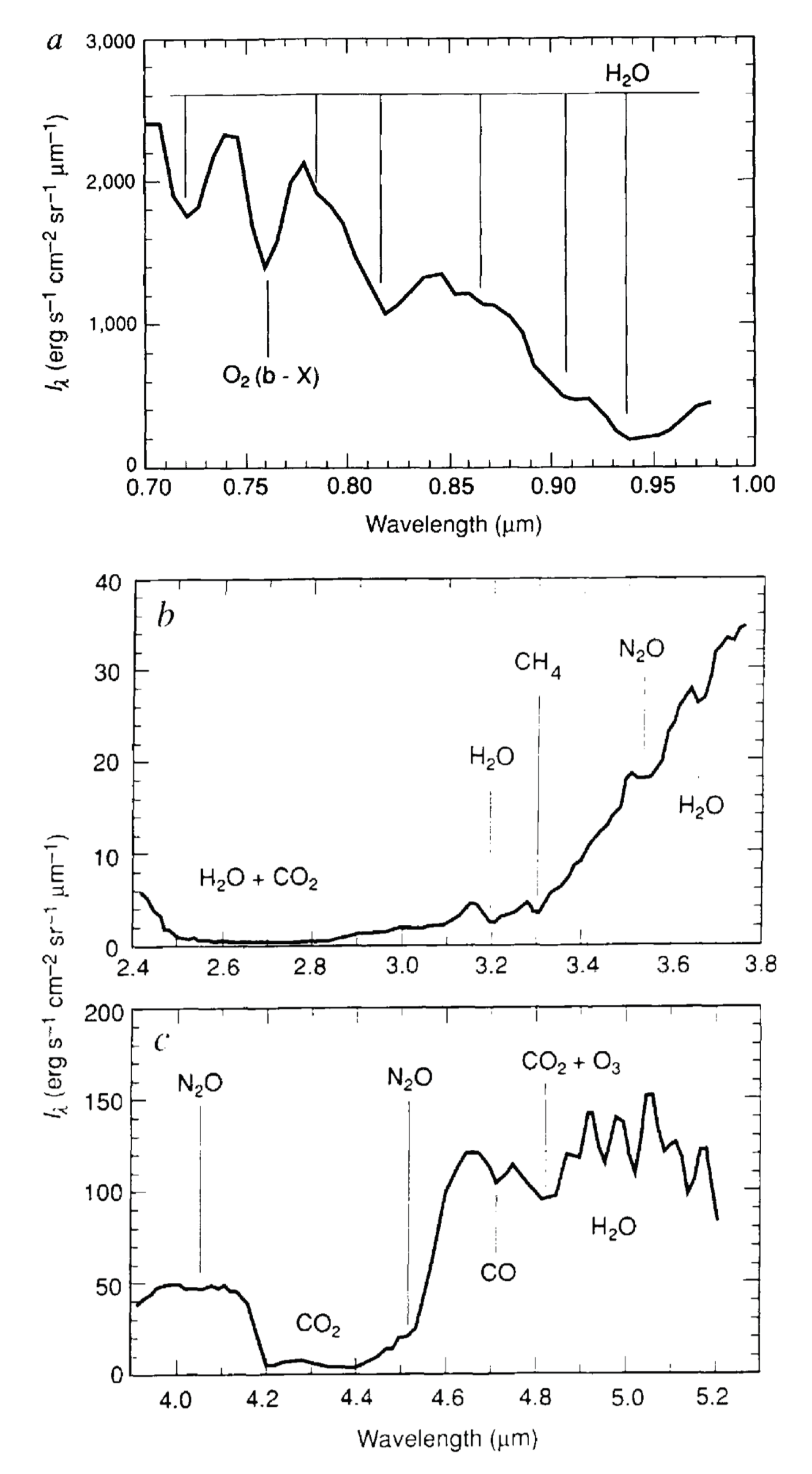
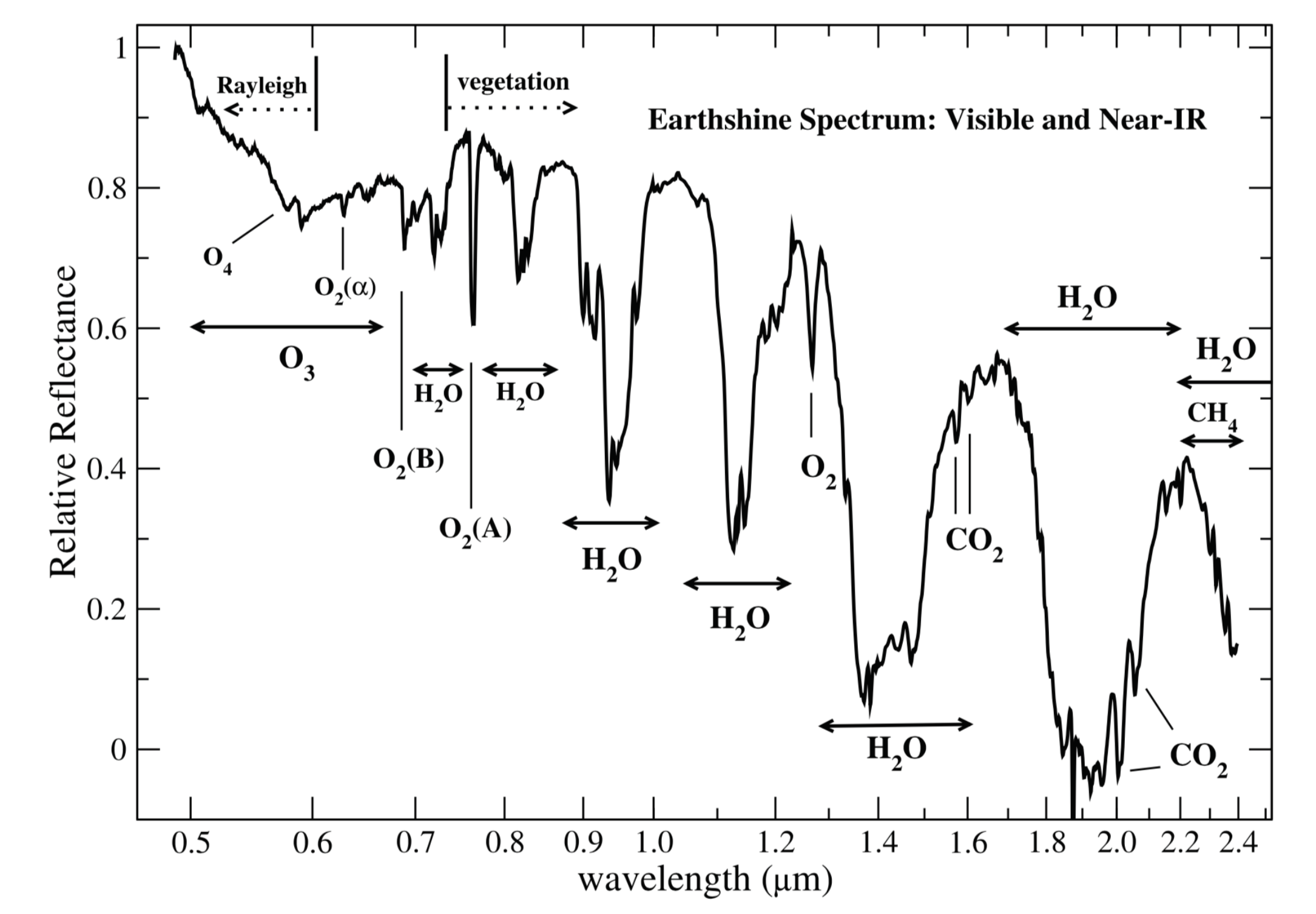
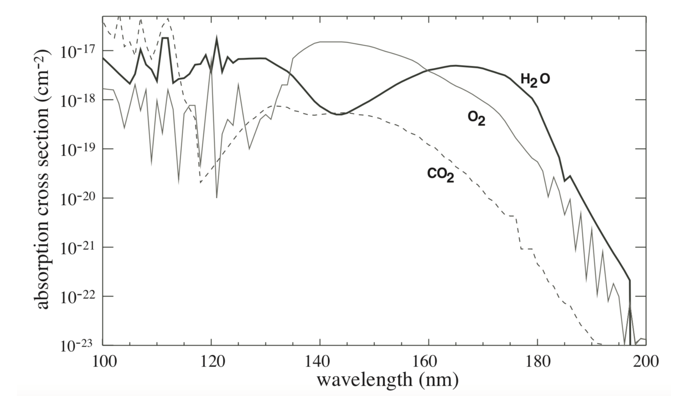
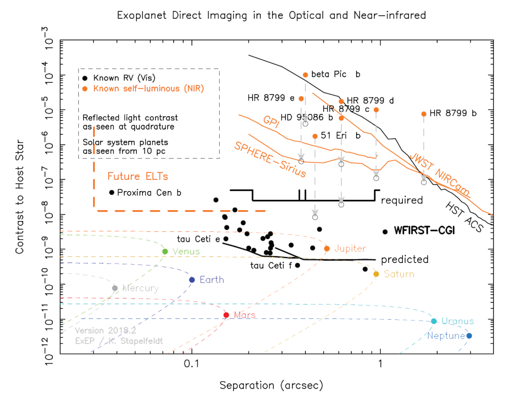
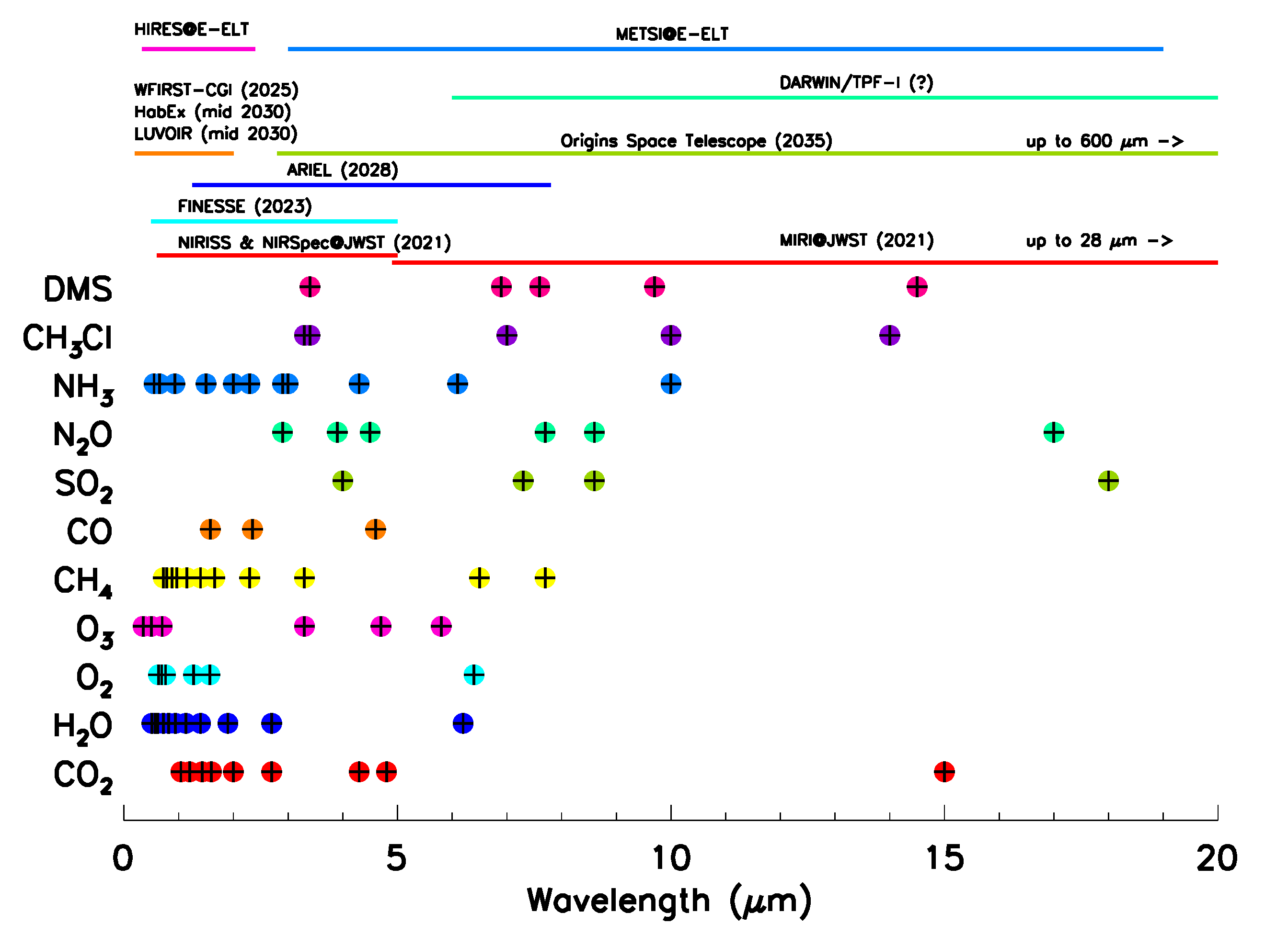
Table 1.
Aerobic Chemotrophy: summary of redox reaction by-products. Modified by [12].
Table 1.
Aerobic Chemotrophy: summary of redox reaction by-products. Modified by [12].
| Reductant | Oxidant | Output | Comment |
|---|---|---|---|
| Oxidation of Organic Matter | |||
| CHO | O | CO, HO | |
| Hydrogen Oxidation | |||
| H | O | HO | |
| H | HO | HO | |
| Sulfur Compound Oxidation | |||
| HS | O | SO | |
| HS | O | S | |
| S | O | SO | |
| S | O | SO | |
| Iron Oxidation | |||
| Fe | O | Fe, OH | |
| Ammonia Oxidation | |||
| NH | O | NO, HO | Acqueous (Nitrite) |
| NH | O | NO, HO | Acqueous (Nitrite) |
| NO | O | NO | Biological/Abiological |
Table 2.
Anaerobic chemotrophy: summary of redox reaction by-products. Modified by [12].
Table 2.
Anaerobic chemotrophy: summary of redox reaction by-products. Modified by [12].
| Reductant | Oxidant | Output | Comment |
|---|---|---|---|
| Denitrification | |||
| H | NO | NO, HO | Biological/Abiological |
| H | NO | NO, HO | Weak spectral feature |
| H | NO | NO, HO | Weak spectral feature |
| H | NO | N, HO | Metabolic product |
| Fe | NO | NO, Fe | Weak spectral feature |
| Fe | NO | NO, Fe | Weak spectral feature |
| Fe | NO | NO, Fe | Weak spectral feature |
| Fe | NO | N, Fe | Metabolic product |
| Iron Reduction | |||
| Organics | Fe | Fe | Anaerobic bacteria, precipitating minerals |
| H | Fe | Fe, Fe | Precipitating minerals |
| Sulfur Reduction | |||
| Organics | SO | SO, SO, H, CO | |
| H | SO | SO, SO, H | |
| H | SO | SO, H | |
| H | SO | S, H | |
| H | SO | HS, H | |
| CH | SO | HS, CO | |
| Methanogenesis | |||
| Organics | CO | CH, HO | |
| H | CO | CH, HO | Abiotic Pathway |
| Anammox | |||
| NH | NO | N, HO | |
| NH | NO | N, HO | |
| NH | NO | N, HO | |
| NH | NO | N, HO | |
Table 3.
Phototrophy: summary of photosynthetic reaction by–products.
| Input | Radiation | Output | Comment |
|---|---|---|---|
| Oxigenic Photosynthesis | |||
| HO | O | Solid biosignature | |
| Anoxygenic Photosynthesis | |||
| HS | S | ||
| SO | HSO | ||
| S | HSO | ||
| H | HO | ||
| Fe | Fe | ||
| NO | NO | ||
Table 4.
Main characteristics of super Earths orbiting binary and multiple star systems. Data are taken by (Schwarz et al. [110], http://www.univie.ac.at/adg/schwarz/multiple.html).
Table 4.
Main characteristics of super Earths orbiting binary and multiple star systems. Data are taken by (Schwarz et al. [110], http://www.univie.ac.at/adg/schwarz/multiple.html).
| System | S | D [pc] | Orb. Type | a[au] | a[au] | M/MM | mM | Method |
| Binary star systems | ||||||||
| OGLE-2013-BLG-o341 b | ?/? | − | − | 0.702 | − | − | 1.57 | -Lens |
| Kepler 68 c | G/? | 135.0 | S | 1450 | 0.0906 | 1.08/0.175 | 2.20 | Transit |
| Kepler 68 b | 0.0617 | 5.98 | Transit | |||||
| K2-288 b | M2V/M3V | 69.3 | S | 54.8 | 0.164 | 0.52/0.33 | 2.83 | Transit |
| GJ 676 d | M0V/M3.5V | 16.45 | S | 800 | 0.0413 | 0.71/0.17 | 4.40 | RV |
| Gliese 15 b | M2V/M3.5 | 3.6 | S | 93 | 0.072 | 0.38/0.15 | 5.35 | RV |
| 55 Cnc e | G8V/M3.5-4V | 1302 | S | 1050 | 0.0156 | 0.95/0.13 | 8.20 | Transit |
| Kepler-453 AB b | ?/? | P | 0.1848 | 0.790 | 0.94/0.19 | 9.43 | Transit | |
| Multiple star systems | ||||||||
| System | S | D[pc] | Orb. Type | a[au] | a[au] | MM | mM | Method |
| Cen AB/Prox Cen b System | ||||||||
| Alpha Cen A | G2V / | 1.1 | ||||||
| Alpha Cen B | K1V / | 0.934 | ||||||
| Prox Cen b | M5.5V | 1.30 | 8700 | 0.0485 | 0.12 | 1.26 | RV | |
| Gliese 667 ABC System | ||||||||
| Gliese 667 A | K5V/ | 0.73 | ||||||
| Gliese 667 B | K3V/ | 0.69 | ||||||
| Gliese 667 C b | M1.5V | 43.03 | 230 | 0.0505 | 0.33 | 5.54 | RV | |
| Gliese 667 C c | 0.125 | 3.74 | RV | |||||
| Gliese 667 C d | 0.276 | 5.03 | RV | |||||
| Gliese 667 C e | 0.213 | 2.67 | RV | |||||
| Gliese 667 C f | 0.156 | 2.67 | RV | |||||
| Gliese 667 Cg | 0.549 | 4.56 | RV | |||||
Table 5.
Summary of biosignature classes with pros and cons.
| Biosignatures | Example | Pros | Cons |
|---|---|---|---|
| Inorganic Gases | O; O; CH | Detectable | Also abiotic |
| process | |||
| Organic Gases | DMS; isoprene etc. | Only bio by–product | Small Concentration |
| Many different Compounds | |||
| Photopigments | Chlorophyll | Unique | Complex in detecting |
| (surface reflectance) | and dependent on evolution | ||
| Industrial | CF; CClF | complex evolved | Small Concentration |
| and polluting life |
© 2019 by the authors. Licensee MDPI, Basel, Switzerland. This article is an open access article distributed under the terms and conditions of the Creative Commons Attribution (CC BY) license (http://creativecommons.org/licenses/by/4.0/).
Share and Cite
MDPI and ACS Style
Claudi, R.; Alei, E. Biosignatures Search in Habitable Planets. Galaxies 2019, 7, 82. https://doi.org/10.3390/galaxies7040082
AMA Style
Claudi R, Alei E. Biosignatures Search in Habitable Planets. Galaxies. 2019; 7(4):82. https://doi.org/10.3390/galaxies7040082
Chicago/Turabian StyleClaudi, Riccardo, and Eleonora Alei. 2019. "Biosignatures Search in Habitable Planets" Galaxies 7, no. 4: 82. https://doi.org/10.3390/galaxies7040082
Note that from the first issue of 2016, this journal uses article numbers instead of page numbers. See further details here.