Article

Optimal PID Controllers for AVR Systems Using Hybrid Simulated Annealing and Gorilla Troops Optimization

1
Smart Grids Research Group, Center of Research Excellence in Renewable Energy and Power Systems, King Abdulaziz University, Jeddah 21589, Saudi Arabia
2
Department of Electrical and Computer Engineering, Faculty of Engineering, King Abdulaziz University, Jeddah 21589, Saudi Arabia
3
Department of Electrical and Computer Engineering, Faculty of Engineering, K. A. CARE Energy Research and Innovation Center, King Abdulaziz University, Jeddah 21589, Saudi Arabia
4
Faculty of Electrical Engineering, University of Montenegro, Podgorica 81000, Montenegro
5
Electrical Engineering Department, College of Engineering, Prince Sattam bin Abdulaziz University, Wadi Addawaser 11991, Saudi Arabia
6
Electrical Engineering Department, Aswan Faculty of Engineering, Aswan University, Aswan 81542, Egypt
7
Department of Electrical Engineering, Valley High Institute of Engineering and Technology, Science Valley Academy, Qalyubia 44971, Egypt
*
Author to whom correspondence should be addressed.
Fractal Fract. 2022, 6(11), 682; https://doi.org/10.3390/fractalfract6110682
Submission received: 27 September 2022 / Revised: 9 November 2022 / Accepted: 14 November 2022 / Published: 18 November 2022
(This article belongs to the Special Issue Advances in Fractional-Order PID Controllers)

Abstract

:
In the literature, all investigations dealing with regulator design in the AVR loop observe the AVR system as a single input single output (SISO) system, where the input is the generator reference voltage, while the output is the generator voltage. Besides, the regulator parameters are determined by analyzing the terminal generator voltage response for a step change from zero to the rated value of the generator voltage reference. Unlike literature approaches, in this study, tuning of the AVR controllers is conducted while modeling the AVR system as a double input single output (DISO) system, where the inputs are the setpoint of the generator voltage and the step disturbance on the excitation voltage, while the output is the generator voltage. The transfer functions of the generator voltage dependence on the generator voltage reference value and the excitation voltage change were derived in the developed DISO-AVR model. A novel objective function for estimating DISO-AVR regulator parameters is proposed. Also, a novel metaheuristic algorithm named hybrid simulated annealing and gorilla troops optimization is employed to solve the optimization problem. Many literature approaches are compared using different regulator structures and practical limitations. Furthermore, the experimental results of 120 MVA synchronous generators in HPP Piva (Montenegro) are presented to show the drawbacks of the literature approaches that observe generator setpoint voltage change from zero to the rated value. Based on the presented results, the proposed procedure is efficient and strongly applicable in practice.

1. Introduction

In traditional electric energy systems (EES), which were dominantly based on producing electric energy from hydro, thermal and nuclear power plants, the usual direction of energy was from production facilities to consumers. Therefore, voltage regulation was achieved through transformers, capacitors, batteries, and automatic voltage regulators of synchronous machines. In these systems, the automatic voltage regulators (AVRs) were of the mechanical type, contributing to the inertia of the system’s response. Nowadays, integrating different renewable energy sources into EES has led to the fact that EES are currently perhaps the most complex dynamic systems in the world from the viewpoint of the number of elements, dimensionality, distribution, management, and regulation. Therefore, it is essential to maintain the voltage at each node within its permitted limits, especially at the generators [1].

1.1. Literature Review

In traditional and modern EES, synchronous generators (SGs) represent the leading and most critical voltage-regulation devices [2]. At present, voltage regulation is achieved in microprocessor technology using AVRs [3], i.e., excitation systems [4]. The AVR loop includes a large number of devices/elements: a synchronous machine, exciter, amplifier, controller, and numerous sensors, which are coupled into a single regulation contour together with other signals such as the value of the excitation current and generator currents, VHz signal, power system stabilizer (PSS) signal, and others. The common structure of the AVR system is depicted in Figure 1 [5], where e denotes the error signal, i.e., the difference between the reference voltage Vref and the terminal voltage Vt.
Modeling, work analysis, testing, and design of AVR systems are highly complex due to many elements and their non-linearity [6,7,8,9,10,11,12]. For this reason, each element of the AVR contour is usually approximated, along with being described using possible simple transfer functions in the literature [8,13,14,15,16,17], where each element, except the controller, is represented using transfer functions of the first order [5,12,18,19,20,21,22,23,24]. However, some studies also show that the generator in AVR loops is represented by a third-order system [25]. The use of the third-order generator model complicates the analysis of the system. On the other hand, it respects a more accurate machine model. Moreover, some publications also use generator models presented via fuzzy logic, neural networks, and the like [25,26].
All the previously cited works deal with estimating regulator parameters or selecting new regulator structures. The most often employed regulator in AVR loops is the ideal proportional-integral-derivative (PID) regulator, which is characterized by three gains—proportional, integral, and differential (Kp, Ki, and Kd) [13,21,27,28]. However, as the ideal controller is impossible to be realized practically, publications also consider a real PID controller, which, in addition to the previous gains, also has a variable that represents the filter coefficient (denoted as N) [6,29,30]. Namely, in this type of regulator, the derivative action is filtered. Besides, there is also the fractional-order PID (FOPID) regulator, in which the functional routine of the ideal PID is improved by adding fractional calculus into the typical structure of the PID controller [8,25,31,32,33]. Therefore, in FOPID, we have two additional variables μ, and λ. Furthermore, recent studies investigate another amendment of the ideal PID regulator, the so-called PID with second-order derivative, or PIDD2 [6,34], or a mix between FOPID and PIDD2 called fractional-order proportional-integral-derivative plus the second-order derivative controller (FOPIDD2) [35]. Unlike the ideal PID regulator, the PIDD2 structure has one extra parameter to be four in total: Kp, Ki, Kd, and Kd2. Figure 2 shows the mathematical formulations of the mentioned regulators, where s represents the Laplace operator variable.
The parameters of regulators were estimated by minimization of the corresponding criterion function (or objective function) to achieve the best possible response, i.e., the desired response of the generator voltage when the reference value changed its value from 0 to 1 per unit (p.u) (nominal value). The most frequently used functions are depicted in Figure 3. ITAE represents the time multiplied by the absolute value of the error [24], IAE represents the integral of the absolute value of the error [31], ITSE is the integral of time multiplied by weighted squared error [21], ISE is the integral of squared error [6], ZLG is a well-known objective function named by the name of the author who first defined it (Zwe-Lee Gaing [5]), OF is an abbreviation for the criterion function of the composition of ITSE and ZLG [28] and so on. For ZLG and OF, β and μ represent constants, while ESS denotes the steady state error, ts denotes the settling time, and tr denotes the rise time. It is apparent that no sole objective function is used in the literature to estimate the parameters of all PID controllers.
In the literature, the optimal tuning of the regulator parameters relies on employing meta-heuristic algorithms such as future search algorithm (FSA) [9], hybrid evolutionary algorithm (HEA) [18], whale optimization algorithm (WOA) [13], combined GA-bacterial foraging (GA-BF) [10], chaotic yellow saddle goatfish algorithm (CYSGA) [8], teaching–learning-based optimization (TLBO) [36], simulated annealing-manta ray foraging optimization algorithm (SA-MRFO) [6], local unimodal sampling algorithm (LUSA) [19], particle swarm optimization (PSO) [5], simplified PSO (SPSO) [24], craziness based PSO (CRPSO) [17], ant colony cptimization (ACO) [14], combined GA and PSO (GAPSO) [27], invasive weed optimization (IWO) [37], sine cosine algorithm (SCA) [32], enhanced crow search algorithm (ECSA) [11], symbiotic organisms search algorithm (SOSA) [38], artificial bee colony (ABC) [21], taguchi combined genetic algorithm (TCGA) [39], chaotic optimization algorithm (COA) [39], improved kidney-inspired algorithm (IKIA) [40], gradient-based optimization algorithm (GBSA) [41], hybrid equilibrium optimizer (HEO) [41], arithmetic optimization algorithm (AOA) [12], improved artificial bee colony algorithm (IABCA) [31], equilibrium optimizer algorithm (EOA) [22], chaotic multi-objective optimization (CMOO) [33], cuckoo search (CS) [16], differential evolution (DE) [21], chaotic ant swarm (CAS) [15], and imperialist competitive algorithm (ICA) [42], chaotic yellow saddle goatfish algorithm (CYSGA) [43], improved Lévy flight distribution algorithm (ILFDA) [44], memorizable-smoothed functional algorithm (MSFA) [45], Lévy flight-based reptile search algorithm (LFRSA) [46], and Rao algorithm [47]. It can be noted that the problem of estimating the parameters of the regulator is a major problem and is represented in many publications. Many algorithms have been tested for this purpose, but their large number and varieties show that the optimal algorithm has not yet been found.

1.2. Paper Novelty and Idea

All the previously published works have one common mutual access. Namely, the parameters are determined to form a step disturbance from 0 to 1 reference value of the generator voltage. However, in practice, such a way of energizing the generator to its nominal value is neither possible nor realistic. Moreover, such a method would damage the machine itself, especially the excitation winding, which should be several times higher than the nominal value of the excitation voltage [48]. A comprehensive explanation of the stated claim is introduced in the following sections. Furthermore, experimental results for 120 MVA from Hydro Power Plant Piva start in terms of start excitation will be presented in this paper in order to confirm the drawbacks of many literature approaches.
Second, the literature examines the system’s robustness when the excitation voltage changes while analyzing the system’s behavior and stability. However, these approaches do not include excitation voltage change during regulator parameter design. Today’s excitation systems are based on the application of thyristor bridges [4]. A small error in the control angle of the thyristor ignition can cause changes in the excitation voltage, which affects the generator voltage. Unlike the literature, in this work, the regulator parameters are estimated considering the allowed generator reference voltage changes and potential changes in the excitation voltage. In this way, the regulator’s designed parameters will help the generator eliminate unwanted changes in the excitation voltage.
Thirdly, the paper will present a new metaheuristic algorithm of a hybrid nature, which aims to determine the parameters of the regulator efficiently. The idea is to connect two algorithms, one of which shows exceptional characteristics for searching unknown parameters, and the other has confirmed characteristics for hybridization from the point of view of defining the initial values of iterative processes.

1.3. Paper Contribution

The core contributions of this study are summarized as follows:
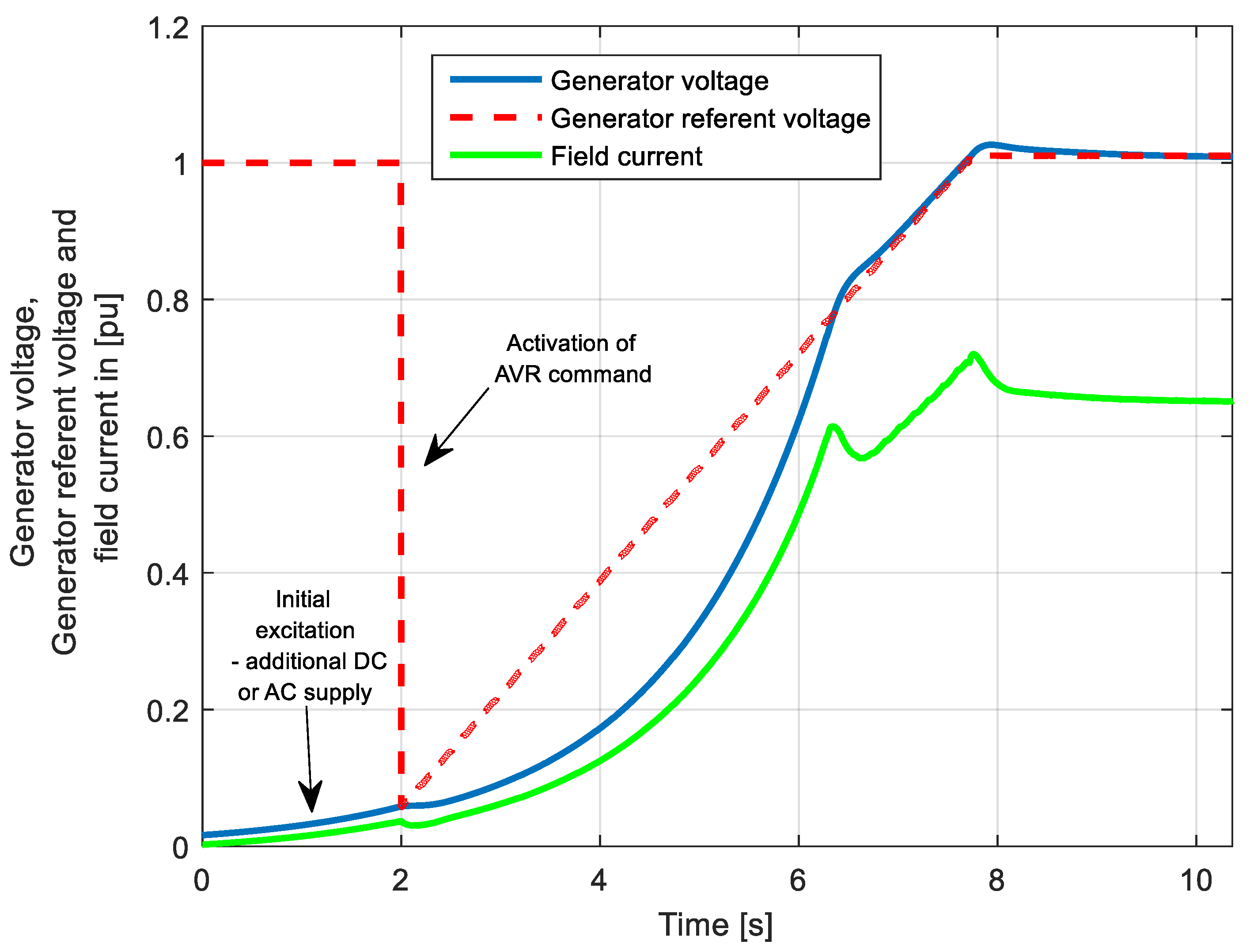
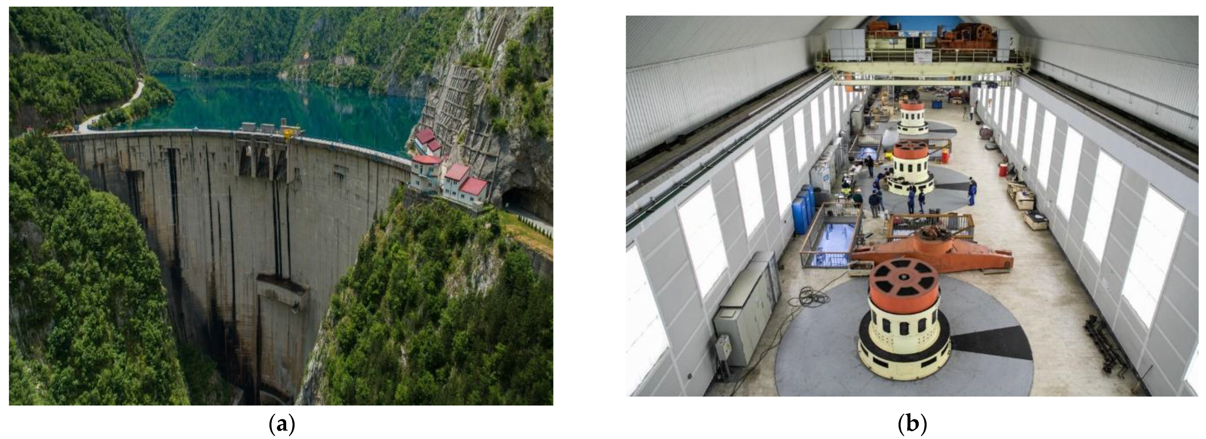
  • The practical implementation of starting the generator is explained in detail by presenting the experimentally measured output of the generator voltage, excitation voltage, and excitation current.
  • A new approach to solving the estimation problem of regulator parameters is presented. It considers the change in the generator voltage within the permitted values of the generator voltage and the change in the excitation voltage in real cases;
  • Unlike the literature, the system is modeled as a DISO system rather than the common SISO one;
  • The DISO model of the AVR system is presented for both generator and excitation voltage output;
  • A novel metaheuristic algorithm named hybrid simulated annealing and gorilla troops optimization is proposed;
  • A new fitness function is employed for parameter estimation. It considers the change in the generator voltage triggered by the changes in the reference value of the generator voltage and in the excitation voltage.

1.4. Paper Organization

This manuscript is organized into eight sections. Section 2 presents the commonly used AVR description and represents it as a DISO system. A short note about synchronous machine starting estimation is given in Section 3. Section 4 introduces the proposed novel metaheuristic algorithm. Simulation results when the excitation voltage is not considered are presented in Section 5. The simulation results that address the excitation voltage limitation are presented in Section 6. Additional tests are presented in Section 7, and finally, the concluding remarks are given in Section 8.

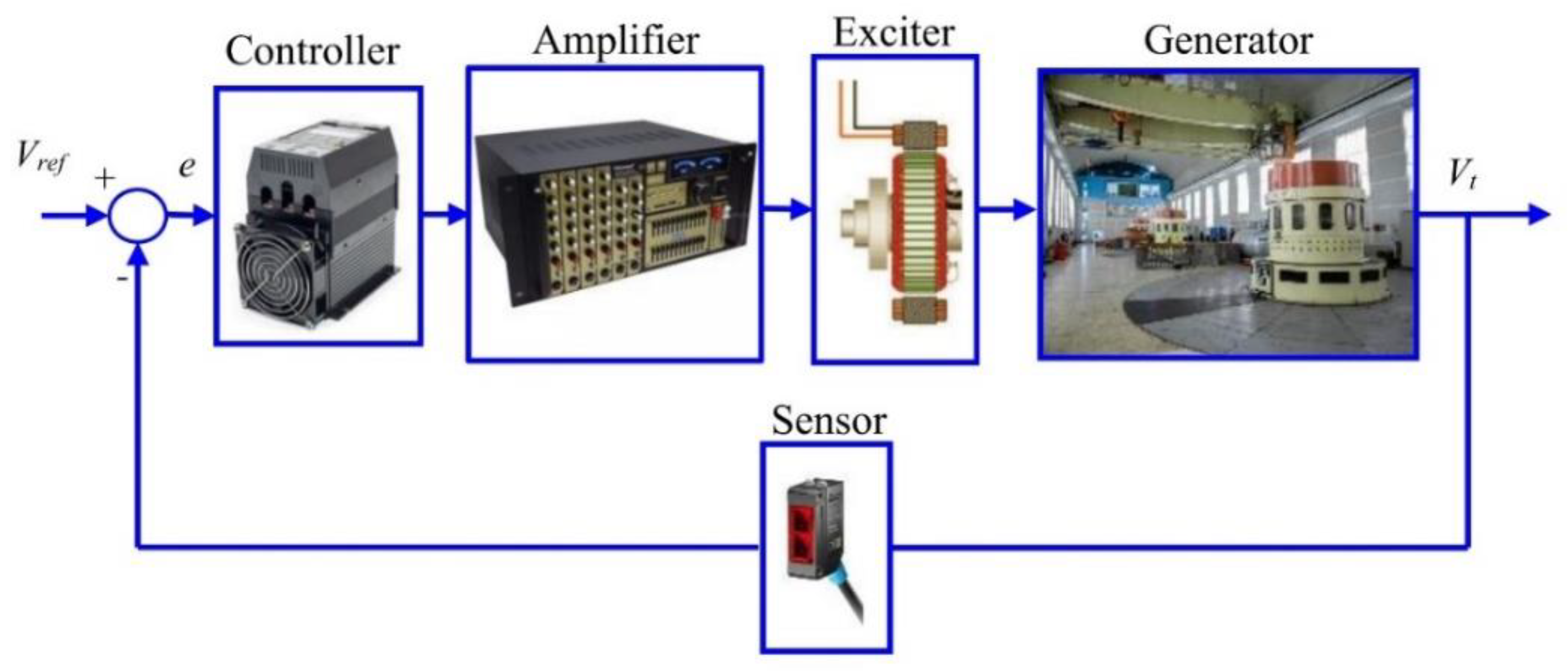
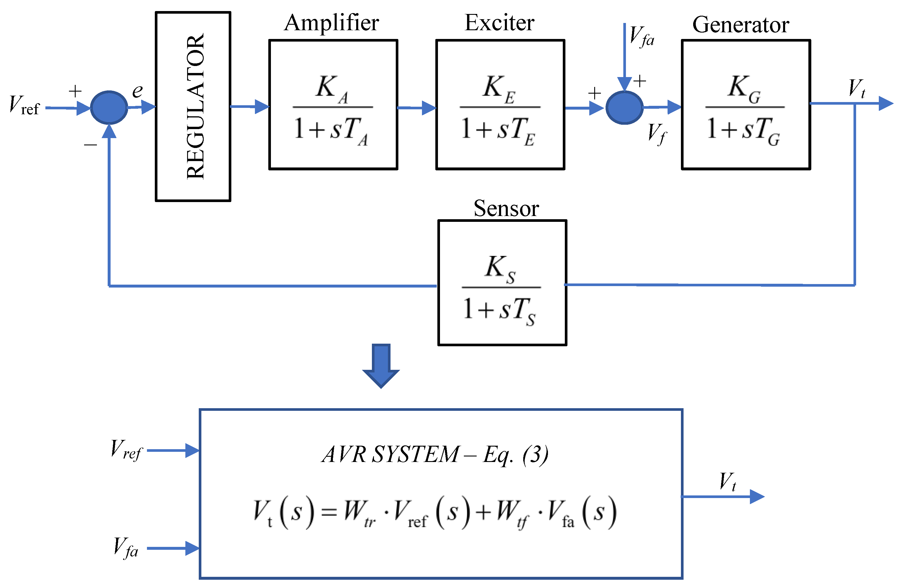
2. Proposed DISO-Model of the AVR

The main function of AVRs is maintaining the generator voltage on the predefined value level (generator reference value) under all operating conditions. Also, its function is to lessen the system voltage variation under abnormal conditions—faults, short circuits, load fluctuation, and others. The AVR model includes components represented via a first-order transfer function. Each transfer function consists of the unitless gain values (denoted K) and the time constant values (denoted T) given in seconds.
Figure 4 represents the AVR model with two input signals (Vref stands for the generator reference voltage, Vfa represents the additional field voltage, and Vt represents the generator terminal voltage). Suffix A represents the amplifier, E represents the exciter, G represents the generator, and S represents the sensor.
Based on Figure 4, the following equation can be derived in the Laplacian domain:
E = V r e f ( s ) W S V t ( s ) , V t ( s ) = W G ( V f a + W E W A R E G E ) .
By solving these equations, one can obtain the following expression, where REG is a regulator of any type:
V t ( s ) = W G W E W A R E G 1 + W G W S W E W A R E G V r e f ( s ) + W G 1 + W G W S W E W A R E G V f a ( s ) , W G = K G 1 + s T G , W E = K E 1 + s T E , W S = K S 1 + s T S , W A = K A 1 + s T A .
In simple form, the previous equation can be expressed as follows:
V t ( s ) = W t r V r e f ( s ) + W t f V f a ( s ) , W t r = W G W E W A R E G 1 + W G W S W E W A R E G , W t f = W G 1 + W G W S W E W A R E G .
In such a case, the excitation voltage is given as follows:
V f ( s ) = W E W A R E G 1 + W G W S W E W A R E G V r e f ( s ) + 1 1 + W G W S W E W A R E G V f a ( s ) .
Therefore, the change in the generator voltage relies on changes in the generator reference voltage and the field voltage. Thus, we derived the AVR mode similarly to the DISO system (as depicted in Figure 4). Also, this model can be regarded as a DIDO model if one considers the excitation voltage as an output signal. Similarly, one can also derive expressions for the dependence of generator voltage on other signals, such as amplified change or signal from the regulator.

3. Short Notes on Synchronous Generator Starting Excitation

The synchronous machine is the central, if not the most important, component in power systems. These are electric machines whose powers range up to several hundreds of MWs. The start of the synchronous machine is realized under the absolute supervision of numerous sensors, monitoring many quantities. Namely, during the starting process and machine loading, the regulation of the power through the turbine regulation and the voltage through the automatic voltage regulation are intertwined. In the case of large synchronous machines, as with the machines in the EES of Montenegro, excitation of the generator when starting the machine can be realized in two modes—AVR mod (automatic voltage regulation mode) and FCR mod (field current regulation mode). The automatic mode reflects the application of the AVR contour—i.e., regulation of voltage, while the manual mode is realized through the excitation current—i.e., regulation of field current. Excitation of the machine starts after the generator is accelerated to a certain value via the turbine regulation (in the EES of Montenegro, it is set to be 90% of the synchronous speed). Therefore, after the generator speed reaches the appropriate value, one of the modes is activated—the auto mode or the manual mode. However, both modes can be realized in terms of the power supply from the generator branch (called shunt supply) and the power supply from the sub-distribution of the 0.4 kV power plant. Therefore, for the first case (shunt supply), an initial DC or AC (plus rectifier), starting power source is needed to initiate the generator excitation. Therefore, the excitation current follows the generator voltage in the shunt supply. The steps of these potential ways for generator excitation are illustrated in Table 1.
This work presents the experimental results from 120 MVA generators from HPP Piva (see Appendix A) in Montenegro to show the electric generator variables and changes during starting excitation. Namely, the 120 MVA generator has a static excitation system (UNITROL 6000), a self-excited-thyristor-controlled system factory-made by ABB. The generator can be excited via all the presented modes. The control is realized using the microprocessor technique, and the variables can be measured and monitored. In order to show the generator starting excitation, the AVR mode with shunt supply is chosen.
The generator is first accelerated to a speed higher than 90% of the nominal speed and is excited from the additional power supply (DC voltage source). As the generator rotates, its voltage will rise, as well as the field current. After a certain time, the initial DC power is stopped, and the generator starts to be excited via a predefined ramp function for voltage. Therefore, we have a ramp change of the generator reference voltage in the AVR contour. During this change, the field current tracks the generator voltage. After the generator reaches the nominal value, the synchronization system is activated, and the generator is synchronized with the grid voltage. The experimentally measured changes in the reference voltage, real generator voltage, and field current are presented in Figure 5.
Based on the previous explanation and the presented experimental results, it is clear that in real situations, for a high-power synchronous generator, it is impossible to start the machine to full voltage value with a step change of generator reference voltage from 0 to 1 p.u. Consequently, the estimation of regulator parameters observing this step change of generator referent voltage is not realistic.

4. Proposed Procedure for Regulator Design in AVRs

In this section, a proposed procedure for AVR regulator design is presented. Namely, in the first part, we described the idea of this work, i.e., observation of the AVR system as a DISO system, while the second part represents the description of the proposed algorithm used in regulator design.

4.1. Novel Procedure for Parameters Design

It was clear that determining the parameters of the regulator is not realistic if a step change from 0 to 1 p.u of the generator voltage is observed. Also, the observation of the response of the generator voltage under the effect of a step change in the reference value of the generator voltage is not representative.
Besides, the initial signal used to change the generator reference voltage from 0 to 1 p.u causes a significant change in the field voltage. In practice, this signal will cause a very high value of the field voltage to get the appropriate level of the excitation–magnetic field in the machine. However, the excitation winding cannot accept any value of the field voltage because of electrical limitations. Such limitations of the allowed field voltage levels were addressed in [2,41]. Furthermore, the influence of limiting the excitation voltage on the parameters was considered in [41].
Thus, this work proposes a new approach to estimating the regulator parameters, including the generator voltage response analysis when the voltage’s reference value is changed within the limits of the allowed values (from 0.95 to 1.05 p.u).
In addition, our research goal (designing the parameters of the regulator) is to consider the effect of changing the excitation voltage in modern power systems. In modern excitation systems, the excitation voltage is obtained from thyristor rectifiers. It is well known that a small error in the control angle of thyristor rectifiers can significantly change the excitation voltage. For this reason, the effect of the change in the excitation voltage of 50% was investigated.
Therefore, the parameters of the regulator are determined so that the variations in the reference value of the generator voltage in addition to the influence of the change in the excitation voltage, are considered. In practice, the shift in generator setpoint voltage value usually takes place, as with its change, the generator operator determines the value of the reactive power and defines the voltage situation in the connected grid.
Therefore, it can be said that the goal of parameter estimation is to eliminate the disturbance—i.e., canceling its effect of noncontrolled change of excitation voltage. In the mathematical sense, the proposed objective function used for regulator parameters determination has the following form:
O F = ( 1 e β ) ( 50 O S 1 + E S S 1 ) + e β ( t s 1 t r 1 ) + I A E 2 + 10 ( O S 2 + t s 2 ) .
The subscript ‘1’ refers to the change caused by the step change of the generator reference voltage value, while ‘2’ refers to the change of the generator voltage caused by the excitation voltage step change. The subscript “s” represents the settling time, while the subscript “r” represents the rise time. The steady-state error is marked as ESS, and the overshoot as OS.
The proposed transfer function consists of two parts. The first part refers to the change in the generator voltage, which is a consequence of the change in the reference value of the generator voltage. This transfer function represents a form of the well-known and most frequently used objective function from the literature proposed by Zwe-Lee Gaing [5]. The second part of the transfer function refers to the change in excitation voltage. A change in the excitation voltage causes a change in the generator voltage, so the idea of this part of the objective function is to eliminate this effect. The second part of the objective function is taken as the sum of the integral IAE and the effects of the maximum value of the generator voltage change (OS2) caused by the excitation voltage change and the settling time of generator voltage (ts2) under the effect of this disturbance.
It should be emphasized that the analogous way of determining the parameters can be applied when considering the change in the value of the output signal from amplifiers or regulators. Therefore, this work starts with the formation of complex systems to determine the parameters of the regulator while canceling the effects of all potential disturbances.

4.2. Novel Optimization Algorithm for AVR Controllers Design

In this work, a novel hybrid meta-heuristic-based algorithm is proposed. It comprises two dissimilar types of algorithms—Simulated Annealing (SA) [7] and Gorilla Troops Optimizer (GTO) [49]. Both algorithms belong to different types of metaheuristics: SA is an algorithm that provides a single solution (it must be applied to each individual of the initial population), which is further used in iterations in generation and replacement procedures. In contrast, GTO is based on populations initiated from an initial population and then iteratively generates other populations.
This paper considers the hybridization of the GTO algorithm [49] and the SA algorithm [7,50], applying the so-called relay-collaboration strategy. In simple words, in this hybrid process, SA is employed to adjust the GTO algorithm population in its initialization to offer a high-quality initial solution. The purpose of such hybrid algorithms is to increase the convergence speed compared to speeds obtained by other algorithms employed to solve the same problem. The following part will briefly describe both SA and GTO algorithms and their hybridization.
In GTO algorithm, one can assume that a population comprises N rays, where Xi(t) (i = 1, 2,…, N) represents the position of each individual. SA algorithm defines the initial population as represented by the pseudo-code given in Algorithm 1 (the objective function of the optimization problem is denoted by f).
Algorithm 1. Pseudo-code of SA (PCSA)
  •    For each individual
  •    Enter the input data: k = 0, ck = c0, Lk = L0
  •    Xi = rand(bH − bL) + bL
  •    Repeat
  •    For l = 0 to Lk
  •    Generate a solution Xj from the neighborhood of Xi
  •    If f(Xj) < f(Xi) then Xj becomes the current solution (Xi = Xj)
  •    Else Xj will become the current solution with a probability e ( f ( i ) f ( j ) c k )
  •    k = k + 1
  •    Compute Lk and ck
  •    Until ck ≅ 0
where Lk and ck represent the number of transitions and temperature generated at the kth iteration [50], rand signifies a random numbers vector (in the range from 0 to 1), while bH and bL express the design variables’ upper and lower bounds. It is essential to mention that each individual is a vector of d variables being optimized. In this work, optimization variables are the parameters of the controller.
The gorilla troops optimizer algorithm relies on the behavior of a group of gorillas in representing the exploration (EXPr) and exploitation (EXPt) optimization phases. Each individual (a gorilla) in a population forms a potential solution to the problem. EXPr comes first in each iteration and is formulated as follows
G X ( t + 1 ) = { ( U B L B ) r 1 + L B , r a n d < p , ( r 2 C ) X r ( t ) + L H , r a n d 0.5 , X ( i ) L ( L ( X ( t ) G X r ( t ) ) + r 3 ( X ( t ) G X r ( t ) ) ) , r a n d < 0.5 } .
where GX(t+1) and X(t) denote the gorilla positions in t and t+1 iterations, respectively, and UB and LB represent the upper bound and lower bound values, respectively. Also, in Equation (6), the parameter p demonstrates the probability of selecting the EXPr strategy to an unidentified position, and rand, r1, r2, and r3 denote random numbers in the range [0, 1]; Xr(t) and GXr(t) represent random gorillas from X and GX. C, L, and H are determined as follows:
C = F ( 1 t t max ) ,
F = cos ( 2 r 4 ) + 1 ,
L = C l ,
and
H = Z X ( t ) , Z = r a n d [ C , C ] ,
where r4 is a random number in the range [0, 1], and l is a random number in the range [1, 1].
At the end of the EXPr phase, it is necessary to calculate the fitness of all GX solutions. In case the fitness of GX(t) is lower than that of X(t), GX(t) replaces X(t). Silverback denotes the best solution, whose fitness function has the lowest value.
After the EXPr phase ends, the EXPt phase occurs. This phase is controlled by W, which should be predefined. The calculation vector GX(t+1) relies on the value of C, as follows:
G X ( t + 1 ) = { L M ( X ( t ) X s i v e r b a c k ) + X ( t ) ,   i f   C W , X s i l v e r b a c k Q ( X s i l v e r b a c k X ( t ) ) A ,   i f   C < W . } .
In the previous equation, the parameter M can be calculated as follows:
M = ( | 1 N i = 1 N G X i ( t ) | 2 / L ) L 2 .
As can be seen from the previous equations, the EXPt phase contains another two parameters, Q, which expresses the impact force, and A, which expresses the degree of violence, that have the following formulations:
Q = 2 r 5 1 ,
A = β E ,
where
E = { N 1 ,   r a n d 0.5 N 2 ,   r a n d < 0.5 } .
To conduct all the previous calculations, it is necessary to explain the following terms: rand and r5 manifest the random numbers between 0 and 1; β, N1, and N2 are coefficients that should be specified before the optimization process starts.
Like EXPr, each gorilla’s fitness function from GX must be computed after the end of EXPt, and potential replacement should be carried out. Precisely, if f(GX(t)) < f(X(t)), GX(t) replaces X(t). The pseudo-code of the complete SA-GTO algorithm is illustrated in Algorithm 2.
Algorithm 2 Pseudo-code of SA-GTO algorithm (PCSA-GTO)
1. Set parameters of GTO algorithm: N, N1, N2, p, β, and tmax
2. Apply SA algorithm to initialize the population
3. Assess the fitness of each gorilla
4. for t=1 to tmax
5. Bring up-to-date L and C
6. Conduct EXPr and GX(t)
7. Assess the fitness of each gorilla
8. Update the population X(t)
9. Find Silverback
10. end for
11. Print Xsilverback
The complexity of the metaheuristic algorithms can be expressed in the following form:
c o m p e l e x i t y = O ( ( n p + C o f p ) N i ) .
where O denotes the big O notation, n denotes the dimension of the parameter space, p represents the population size, Ni denotes the number of iterations, and Cof denotes the complexity of the objective function. The complexity is approximate and highly depends on the objective function. The hybrid algorithm has a higher complexity s they rely on the two algorithms. There is a different form of hybrid algorithms—for defining the initial condition, in any iteration to check both algorithms, half iteration number of operating one and in the second half to operate the second algorithm, and so on. In our case, complexity is the sum of the complexity of simulated annealing and gorilla troops optimization algorithms, as we used the first algorithm to define the initial value for the second algorithm. Compared with other hybrid algorithms, the proposed algorithm’s complexity is identical.

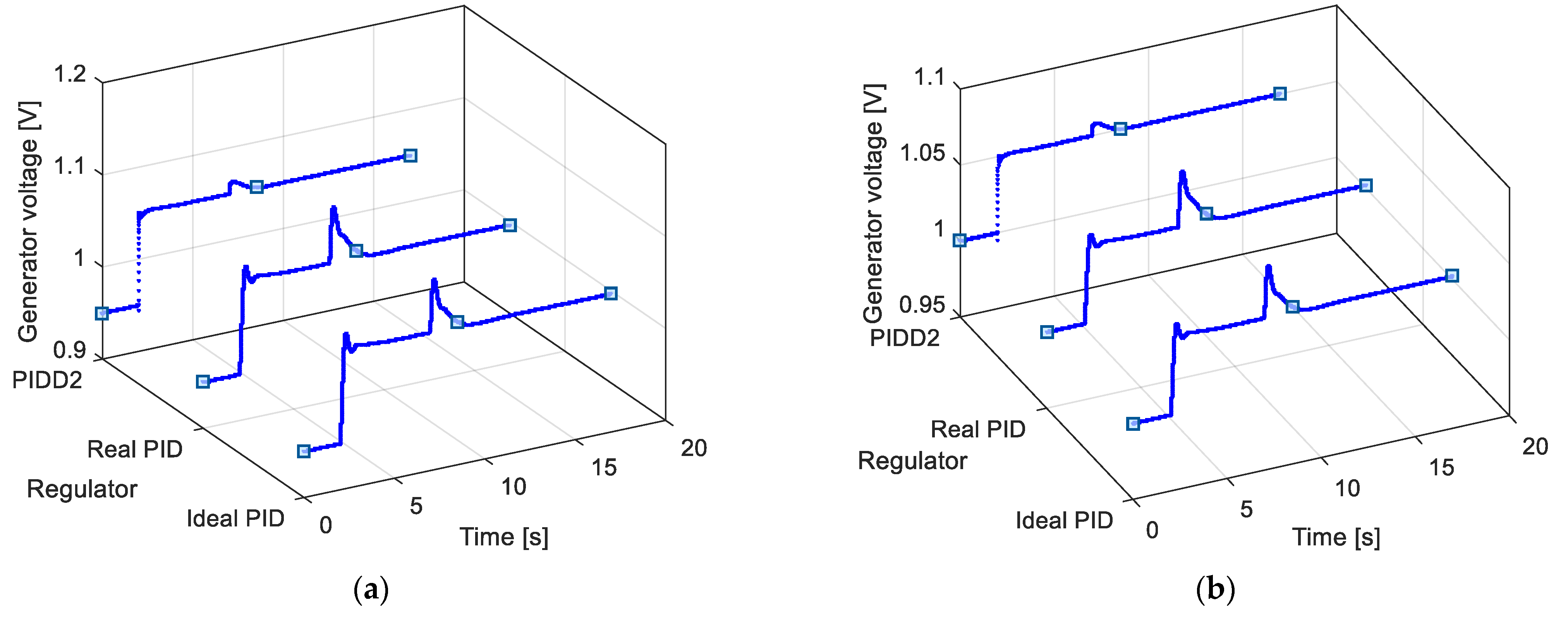
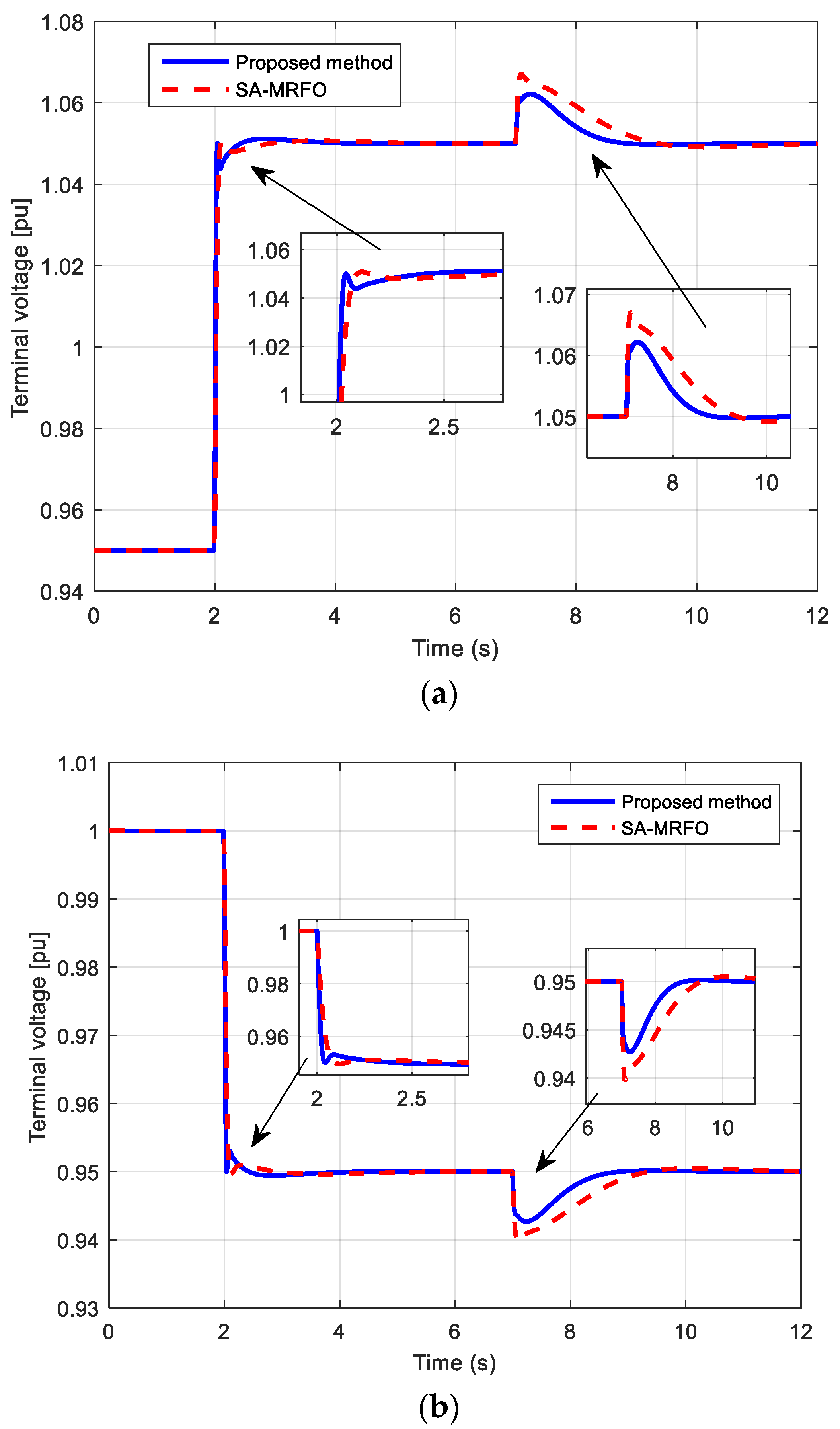
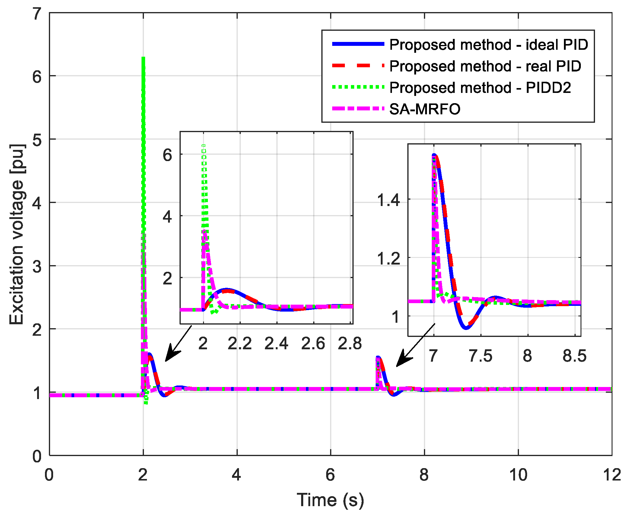
5. Simulation Results with No Limitation of the Excitation Voltage

The results obtained for optimizing different AVR controllers using SA-GTO are presented. Namely, we considered three regulators: ideal PID, real PID, and PIDD2. It should be noted that the SA–GTO algorithm parameters are kept the same for each regulator in all optimization algorithms (maximum iterations number = 100, and the population size = 50). For each regulator, the allowed parameter limits were from 0.1 to 5, except for N in the real PID regulator, whose limits were taken from 100 to 1000.
Figure 6 shows the generator voltage responses when all types of regulators are used for optimal parameters determined by applying the proposed procedure and algorithm (presented in Table 2). The results obtained are summarized and presented in Table 3 in terms of the rise time, settling time, overshoot, and errors in the steady state during the step change of generator reference voltage value and step change of excitation voltage. Index 1 refers to the transient process caused by the change of the generator reference voltage value, and index 2 refers to the transient process caused by the step change in the excitation voltage.
In all investigations, it was assumed that the step change of the excitation voltage is 0.5 p.u. Based on the given responses, it can be noted that the PIDD2 controller enables the highest quality response from the point of view of the transient processes. It can also be seen that PID and real PID provide almost equal responses.
Figure 7 shows the responses of the generator voltage for different step change values and step alterations in the excitation voltage. On the basis of these results, it is clear that PIDD2 enables obtaining responses with better characteristics compared to the responses of systems with real and ideal PID controllers. These figures confirm the system’s robustness to the effect of different step change values and generator and excitation voltage reference values.
Figure 8 shows the generator voltage responses for different system parameters. Namely, this figure shows the test results of the system robustness for different time constants of all components in the AVR system. Each of the used regulators ensures the system’s stability, regardless of the values of the time constants. Moreover, changes in time constants, which in practice represent changes in the components of the AVR structure, cause slight differences in the responses of the generator voltage compared to the case of the nominal parameters of all system components. A detailed comparison of the characteristic values under step change in the generator voltage (from 0.95 to 1.05 p.u) and a change in the excitation voltage of 0.5 p.u for different time components of the system is presented in Table 4.
Therefore, it is notable that a stable response characterizes the system even when dealing with different values of time constants and step changes of the generator and excitation voltages. Therefore, the system’s robustness to the effects of any of the mentioned disturbances, i.e., changes in the AVR structure, is apparent.
To further examine the procedure proposed for determining the regulator’s parameters as well as the system itself, a comparison was made regarding the response metrics to the changes in the reference value of the generator and the excitation voltages in case of using regulators’ parameters whose values were determined by applying numerous algorithms (14 different optimizers) presented in the literature. Table 5 shows the list of the used regulators and the values of their parameters. The generator voltage responses for all algorithms are presented in Figure 9, and the evaluation metrics are given in Table 6.
It is obvious in Figure 9 that the algorithms enable a good system response to the effect of a step change in the reference value of the generator voltage. But, when the value of the excitation voltage changes, which can be understood as a disturbance in the system, substantial and slow transient processes of the generator voltage occur. Therefore, it is clear that the selected values of the regulator parameters do not ensure a prompt rejection of disturbance signals that might exist in the AVR system. Observing these responses, it is clear that SA-MRFO investigated in [6] provides the shortest rise time and settling time compared to the other investigated algorithms. Also, these algorithms provide the smallest overshoot under excitation voltage change. Besides, it is clear that the PIDD2 regulator provides the best responses for the system, i.e., it best contributes to canceling the effect of disturbance signals.
The generator voltage responses are depicted in Figure 10 using the regulator parameters obtained using the proposed method and SA-MRFO presented in [6]. These responses were obtained for changes in the generator voltage reference value and excitation voltage disturbance. Thus, from the responses presented, it is clear that the proposed SA-GTO enables the best system responses.

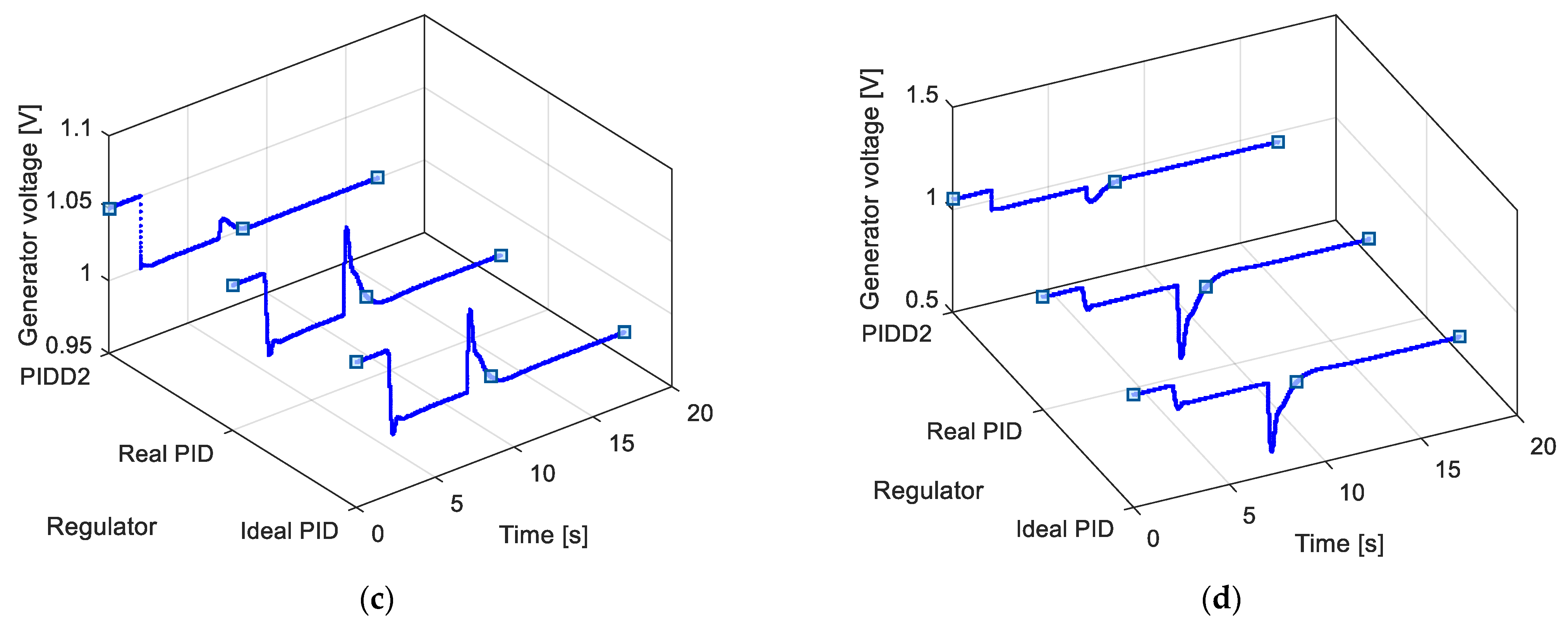
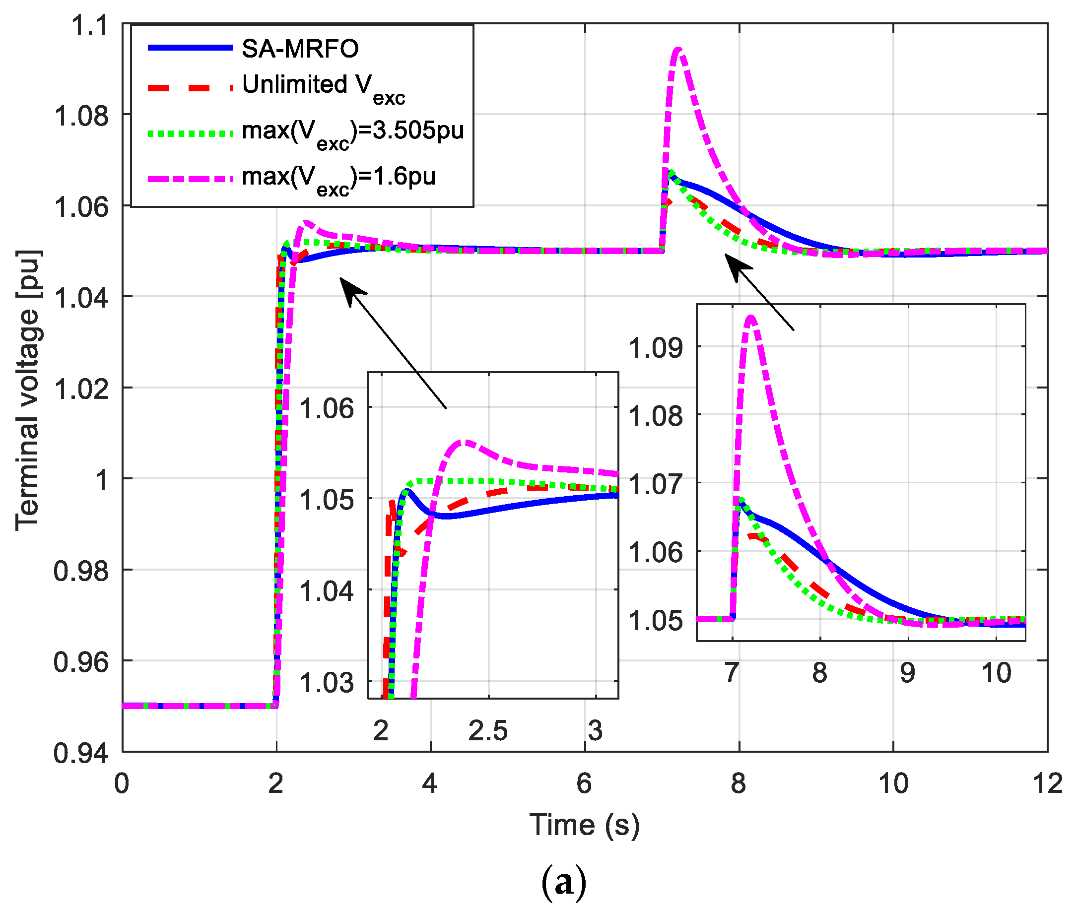
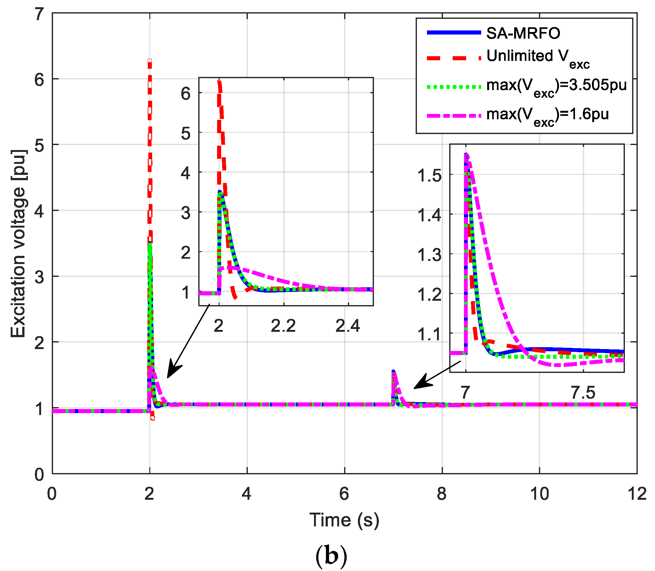
6. Simulation Results with Limitation of the Excitation Voltage

The previously conducted optimization of the regulator parameters and the overall analysis did not consider checking the maximum permissible excitation voltage value that can be formed when the reference value of the generator voltage is changed. Namely, it is known from the literature that the maximum allowed value of excitation voltage during operation ranges from 1.6 to 3 p.u, e.g., it can be from 1.6 to 3 times higher than the nominal value. However, forcing the excitation voltage to values more than 2 p.u is practically not desirable because the forcings will stress the magnetic circuit of the machine [2,41]. Due to the above considerations, an analysis of the excitation voltage values for the regulator parameters presented in Table 5 was carried out.
Figure 11 shows the excitation voltage responses that correspond to changes in the generator voltage for parameters determined by the proposed method/procedure (for the three regulators) and for PIDD2 regulators whose parameters are determined by the SA-MRFO method shown in [6]. It was seen that when the reference value of the generator voltage is changed, there is a considerable increase in the excitation voltage when using the proposed PIDD2 regulator. A similar situation also exists with the PIDD2 regulator from [6]. However, real PID and ideal PID remained within the allowed values. Therefore, if the limitation of the excitation voltage is also observed, it can be concluded that the parameters of the PIDD2 regulator are not well chosen because they do not guarantee the safety of the excitation winding.
For this reason, another procedure to estimate the parameters was executed using the proposed objective function, modified to monitor the excitation voltage. So, if the excitation voltage value exceeds a specific limit, the value of the function will provide an infinite value. Mathematically, the modified objective function (OFn) has the following form:
O F n = { ( 1 e β ) ( 50 O S 1 + E S S 1 ) + e β ( t s 1 t r 1 ) + I A E 2 + 10 ( O S 2 + t s 2 ) if   V e x c < V e x c _ max   for   all   points   if   V e x c V e x c _ max   for   any   points } .
In order to compare with the method presented in [6], the parameters were first estimated for the case that the maximum value of the excitation voltage is 3.505 p.u (maximum value of the excitation voltage corresponding to SA-MRFO). In addition, parameter estimation was performed for the maximum value of the excitation voltage of 1.6 p.u, i.e., for the value of the excitation voltage that ensures safe operation when the reference value of the generator voltage changes. The parameters of the PIDD2 controller obtained using the proposed method for two different values of the maximum excitation voltage are presented in Table 7.
Also, the generator and excitation voltage responses for changes in the generator reference voltage as well as for step load change (0.5 p.u), are illustrated in Figure 12.
A few conclusions can be drawn out while observing these results. First, the proposed method enables better cancellation of the sudden variation of the excitation voltage change, unlike the method in [6] for the same maximum excitation voltage value. Second, the small defined value of the excitation voltage causes a slower response of the generator voltage (increasing excitation voltage cause higher and faster generator voltage rise). Furthermore, this conclusion is the same as the concluding remarks in [41] about the impact of the excitation voltage limitation. Third, the small excitation voltage limitation value causes the generator voltage’s worst response due to the excitation voltage change.
To conclude, the obtained results validate that the proposed parameter estimation method is potent, efficient, and applicable. Furthermore, the importance of the proposed procedure, which implies eliminating the excitation voltage, is demonstrated.

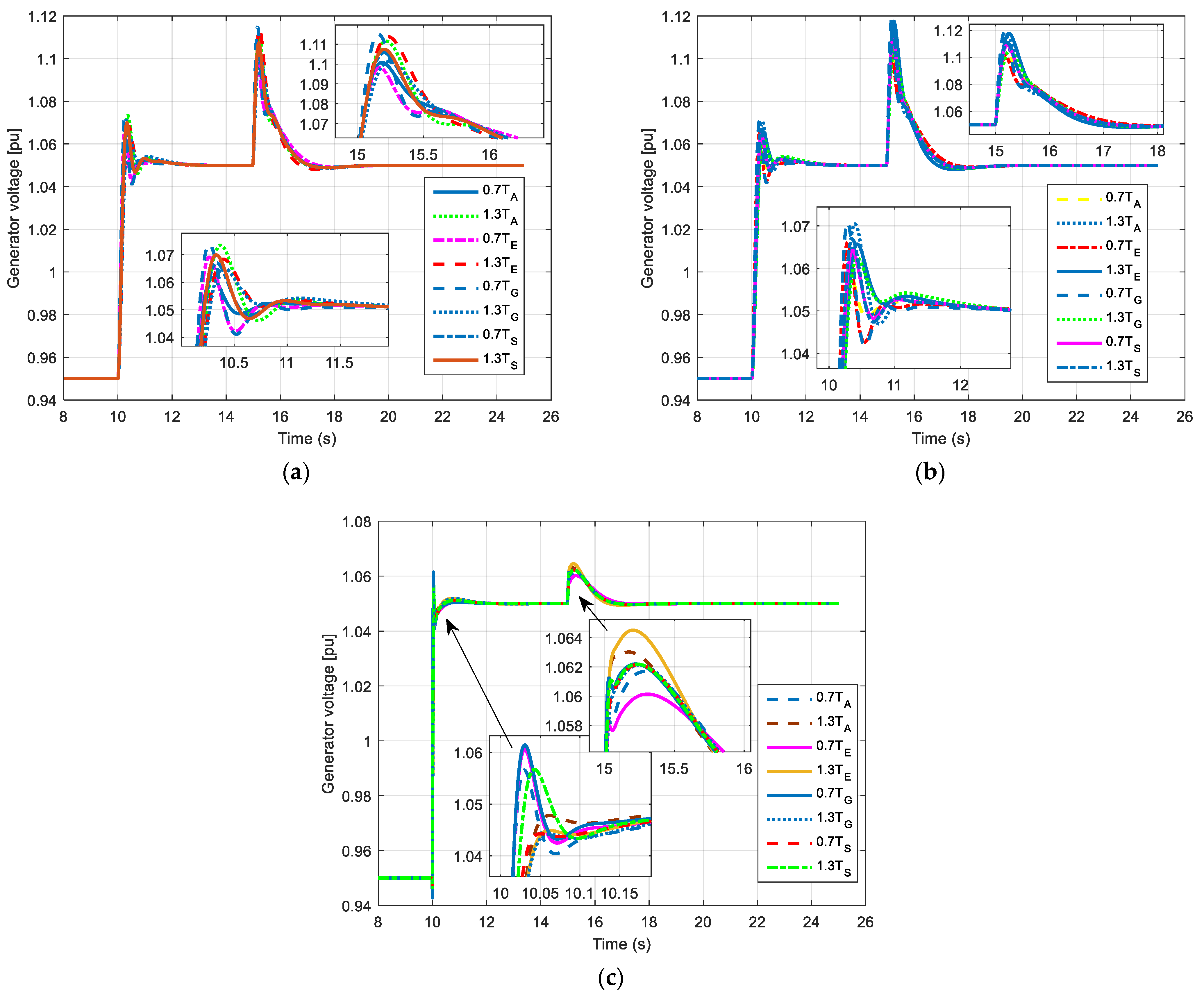
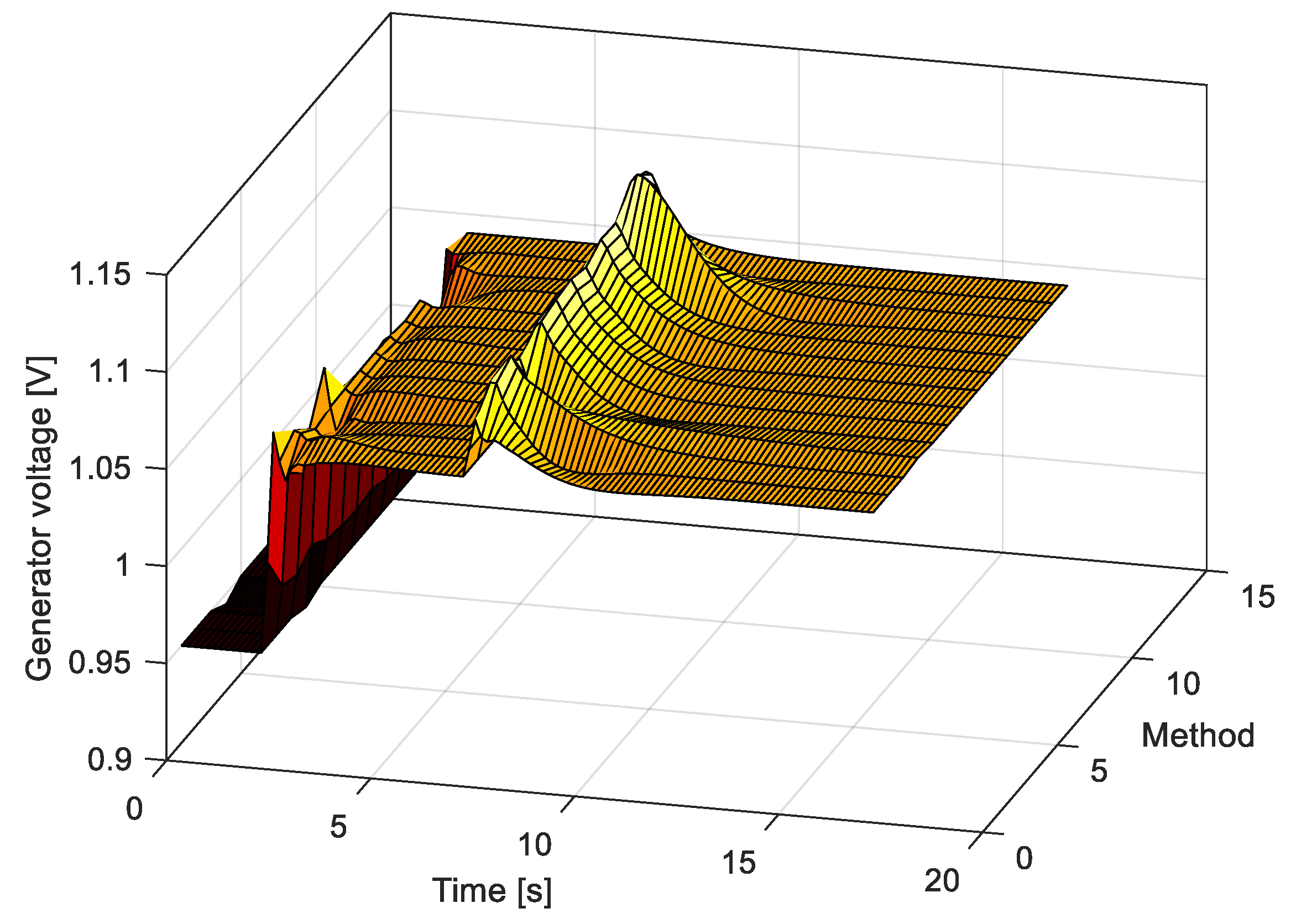
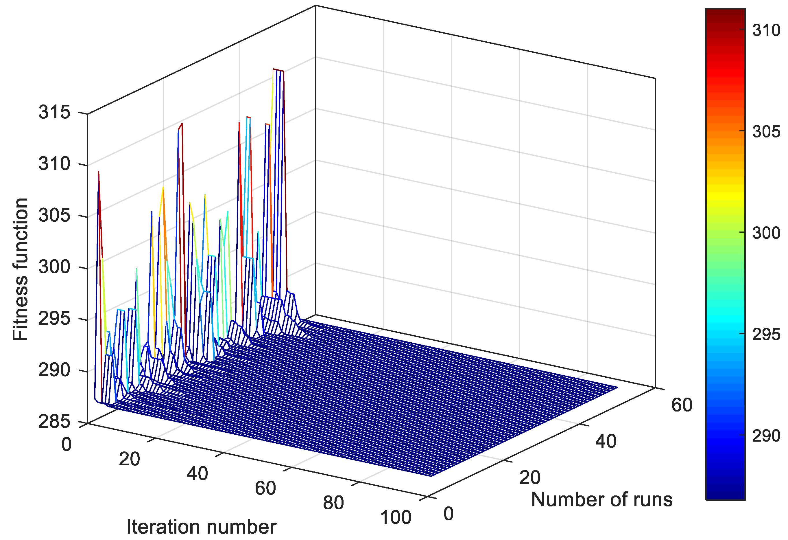
7. Algorithm Testing

To show the advantages of the proposed algorithm over other literature-known algorithms, we also proposed algorithms tests in this work. In this regard, we observed two recent algorithms—the honey badger algorithm (HBA) [51] and GTO [49]. For all algorithm testing, the numbers of population and iterations are set to 100, and 50 independent runs are executed. Figure 13 presents the number of runs—iteration number—fitness function values. Based on this curve, we derived the mean fitness function versus the iteration number curve shown in Figure 14 for all algorithms.
Additionally, different statistical measures of the algorithm’s results are performed and presented in Table 8. As can be seen, all tests provide approximately the same measures (the differences are in some small digits). However, the standard deviation confirms that the proposed algorithm is the best method for regulator parameter design. The same conclusion is supported by the results presented for the Wilcoxon test. Based on all the presented results, it is evident that the algorithm proposed in this study has better statistical features than others.

8. Conclusions and Future Work

This paper deals with determining parameters and the optimal type of regulator in AVR systems. In this regard, we proposed a new procedure for determining the regulator parameters, which considers the step change in the reference value of the generator voltage and the change in the excitation voltage. Namely, unlike literature approaches, the design of the regulator aims to cancel the change in generator voltage that may occur in practical systems. In real systems, the excitation voltage is obtained from thyristor rectifiers, and a small error in the value of the control angle can lead to major problems in voltage regulation.
The proposed procedure was tested for two cases. First, the parameters of three regulators were estimated with no limitation on the excitation voltage. The second case also determines the parameters with these limitations. New objective functions are proposed for both cases. Besides, a new but efficient algorithm for estimating the parameters of the AVR contour regulator has also been refined. A unique contribution of the work was formulating the problem of estimating the regulator parameters as a DISO problem. Accordingly, the transfer functions of the generator voltage dependence on the generator voltage reference value and the excitation voltage change were derived.
According to the author’s knowledge, the subject research represents the initial research in determining the parameters of the regulator, which considers variations in the excitation voltage. Therefore, the potential research constraints are significant. For instance, future work will be oriented toward developing an AVR system model that considers possible disturbances on any elements (output from the regulator, sensor, or amplifier). Therefore, future work will observe the parameter estimation problem as a multi-input-single-output (MISO) problem. Likewise, it is possible to include non-linear restrictions on signals according to their realistic appearance.

Author Contributions

Conceptualization, M.C., M.M. and S.H.E.A.A.; methodology, M.C.; validation, S.A., H.F.S., M.R. and A.A.A.; formal analysis, S.A. and Z.M.A.; investigation, H.F.S., M.R., A.A.A. and Z.M.A.; resources, S.A., H.F.S., M.R. and A.A.A.; data curation, M.C. and S.H.E.A.A.; writing—original draft preparation, M.M. and M.C.; writing—review and editing, S.H.E.A.A.; visualization, M.C. and S.H.E.A.A.; funding, S.A., H.F.S., M.R. and A.A.A. All authors have read and agreed to the published version of the manuscript.

Funding

This publication is based upon work supported by Khalifa University (KU) and King Abdulaziz University (KAU) Joint Research Program Award No KAUKUJRP-1E-2021.

Data Availability Statement

Not applicable.

Conflicts of Interest

The authors declare no conflict of interest.

Appendix A

Figure A1 illustrates the hydropower plant (HPP) Piva and the generators in HPP Piva, Montenegro, where the experiments presented in this work were conducted.
Figure A1. The HPP and the generators in HPP Piva where the experiments were conducted: (a) HPP Piva and (b) generators in HPP Piva, Montenegro.
Fractalfract 06 00682 g0a1

References

  1. Glover, J.D.; Sarma, M.S.; Overbye, T.; Birchfield, A. Power System Analysis and Design, 7th ed.; Cengage Learning: Boston, MA, USA, 2022; ISBN 0357676181. [Google Scholar]
  2. Lipo, T.A. Analysis of Synchronous Machines, 2nd ed.; CRC Press: Boca Raton, FL, USA, 2017; ISBN 9781138073074. [Google Scholar]
  3. Sikander, A.; Thakur, P. A new control design strategy for automatic voltage regulator in power system. ISA Trans. 2020, 100, 235–243. [Google Scholar] [CrossRef] [PubMed]
  4. Nøland, J.K.; Nuzzo, S.; Tessarolo, A.; Alves, E.F. Excitation System Technologies for Wound-Field Synchronous Machines: Survey of Solutions and Evolving Trends. IEEE Access 2019, 7, 109699–109718. [Google Scholar] [CrossRef]
  5. Gaing, Z.-L. A particle swarm optimization approach for optimum design of PID controller in AVR system. IEEE Trans. Energy Convers. 2004, 19, 384–391. [Google Scholar] [CrossRef] [Green Version]
  6. Micev, M.; Ćalasan, M.; Ali, Z.M.; Hasanien, H.M.; Abdel Aleem, S.H.E. Optimal design of automatic voltage regulation controller using hybrid simulated annealing—Manta ray foraging optimization algorithm. Ain Shams Eng. J. 2021, 12, 641–657. [Google Scholar] [CrossRef]
  7. Rodriguez, F.J.; García-Martinez, C.; Lozano, M. Hybrid metaheuristics based on evolutionary algorithms and simulated annealing: Taxonomy, comparison, and synergy test. IEEE Trans. Evol. Comput. 2012, 16, 787–800. [Google Scholar] [CrossRef]
  8. Micev, M.; Ćalasan, M.; Oliva, D. Fractional order PID controller design for an AVR system using Chaotic Yellow Saddle Goatfish Algorithm. Mathematics 2020, 8, 1182. [Google Scholar] [CrossRef]
  9. Elsisi, M.; Soliman, M. Optimal design of robust resilient automatic voltage regulators. ISA Trans. 2021, 108, 257–268. [Google Scholar] [CrossRef] [PubMed]
  10. Kim, D.H.; Cho, J.H. Retraction of “A Biologically Inspired Intelligent PID Controller Tuning for AVR Systems”. Int. J. Control. Autom. Syst. 2011, 9, 814. [Google Scholar] [CrossRef] [Green Version]
  11. Bhullar, A.K.; Kaur, R.; Sondhi, S. Enhanced crow search algorithm for AVR optimization. Soft Comput. 2020, 24, 11957–11987. [Google Scholar] [CrossRef]
  12. Elsisi, M.; Tran, M.Q.; Hasanien, H.M.; Turky, R.A.; Albalawi, F.; Ghoneim, S.S.M. Robust model predictive control paradigm for automatic voltage regulators against uncertainty based on optimization algorithms. Mathematics 2021, 9, 2885. [Google Scholar] [CrossRef]
  13. Mosaad, A.M.; Attia, M.A.; Abdelaziz, A.Y. Whale optimization algorithm to tune PID and PIDA controllers on AVR system. Ain Shams Eng. J. 2019, 10, 755–767. [Google Scholar] [CrossRef]
  14. Blondin, M.J.; Sanchis, J.; Sicard, P.; Herrero, J.M. New optimal controller tuning method for an AVR system using a simplified Ant Colony Optimization with a new constrained Nelder–Mead algorithm. Appl. Soft Comput. 2018, 62, 216–229. [Google Scholar] [CrossRef]
  15. Tang, Y.; Cui, M.; Hua, C.; Li, L.; Yang, Y. Optimum design of fractional order PIλDμ controller for AVR system using chaotic ant swarm. Expert Syst. Appl. 2012, 39, 6887–6896. [Google Scholar] [CrossRef]
  16. Sikander, A.; Thakur, P.; Bansal, R.C.; Rajasekar, S. A novel technique to design cuckoo search based FOPID controller for AVR in power systems. Comput. Electr. Eng. 2018, 70, 261–274. [Google Scholar] [CrossRef]
  17. Mukherjee, V.; Ghoshal, S.P. Intelligent particle swarm optimized fuzzy PID controller for AVR system. Electr. Power Syst. Res. 2007, 77, 1689–1698. [Google Scholar] [CrossRef]
  18. Wong, C.C.; Li, S.A.; Wang, H.Y. Hybrid evolutionary algorithm for PID controller design of AVR system. J. Chinese Inst. Eng. 2009, 32, 251–264. [Google Scholar] [CrossRef]
  19. Mohanty, P.K.; Sahu, B.K.; Panda, S. Tuning and Assessment of Proportional–Integral–Derivative Controller for an Automatic Voltage Regulator System Employing Local Unimodal Sampling Algorithm. Electr. Power Components Syst. 2014, 42, 959–969. [Google Scholar] [CrossRef]
  20. Dos Santos Coelho, L. Tuning of PID controller for an automatic regulator voltage system using chaotic optimization approach. Chaos Solitons Fractals 2009, 39, 1504–1514. [Google Scholar] [CrossRef]
  21. Gozde, H.; Taplamacioglu, M.C. Comparative performance analysis of artificial bee colony algorithm for automatic voltage regulator (AVR) system. J. Franklin Inst. 2011, 348, 1927–1946. [Google Scholar] [CrossRef]
  22. Micev, M.; Ćalasan, M.; Oliva, D. Design and robustness analysis of an Automatic Voltage Regulator system controller by using Equilibrium Optimizer algorithm. Comput. Electr. Eng. 2021, 89, 106930. [Google Scholar] [CrossRef]
  23. Sahib, M.A.; Ahmed, B.S. A new multiobjective performance criterion used in PID tuning optimization algorithms. J. Adv. Res. 2016, 7, 125–134. [Google Scholar] [CrossRef] [PubMed] [Green Version]
  24. Panda, S.; Sahu, B.K.; Mohanty, P.K. Design and performance analysis of PID controller for an automatic voltage regulator system using simplified particle swarm optimization. J. Franklin Inst. 2012, 349, 2609–2625. [Google Scholar] [CrossRef]
  25. Zamani, M.; Karimi-Ghartemani, M.; Sadati, N.; Parniani, M. Design of a fractional order PID controller for an AVR using particle swarm optimization. Control Eng. Pract. 2009, 17, 1380–1387. [Google Scholar] [CrossRef]
  26. Gillard, D.M.; Bollinger, K.E. Neural network identification of power system transfer functions. IEEE Trans. Energy Convers. 1996, 11, 104–110. [Google Scholar] [CrossRef]
  27. Kim, D.H. Hybrid GA–BF based intelligent PID controller tuning for AVR system. Appl. Soft Comput. 2011, 11, 11–22. [Google Scholar] [CrossRef]
  28. Ekinci, S.; Hekimoğlu, B. Improved Kidney-Inspired Algorithm Approach for Tuning of PID Controller in AVR System. IEEE Access 2019, 7, 39935–39947. [Google Scholar] [CrossRef]
  29. Bingul, Z.; Karahan, O. A novel performance criterion approach to optimum design of PID controller using cuckoo search algorithm for AVR system. J. Franklin Inst. 2018, 355, 5534–5559. [Google Scholar] [CrossRef]
  30. Blondin, M.J.; Sicard, P.; Pardalos, P.M. Controller Tuning Approach with robustness, stability and dynamic criteria for the original AVR System. Math. Comput. Simul. 2019, 163, 168–182. [Google Scholar] [CrossRef]
  31. Zhang, D.-L.; Tang, Y.-G.; Guan, X.-P. Optimum Design of Fractional Order PID Controller for an AVR System Using an Improved Artificial Bee Colony Algorithm. Acta Autom. Sin. 2014, 40, 973–979. [Google Scholar] [CrossRef]
  32. Ayas, M.S.; Sahin, E. FOPID controller with fractional filter for an automatic voltage regulator. Comput. Electr. Eng. 2021, 90, 106895. [Google Scholar] [CrossRef]
  33. Pan, I.; Das, S. Frequency domain design of fractional order PID controller for AVR system using chaotic multi-objective optimization. Int. J. Electr. Power Energy Syst. 2013, 51, 106–118. [Google Scholar] [CrossRef] [Green Version]
  34. Sahib, M.A. A novel optimal PID plus second order derivative controller for AVR system. Eng. Sci. Technol. Int. J. 2015, 18, 194–206. [Google Scholar] [CrossRef] [Green Version]
  35. Tabak, A. Maiden application of fractional order PID plus second order derivative controller in automatic voltage regulator. Int. Trans. Electr. Energy Syst. 2021, 31, e13211. [Google Scholar] [CrossRef]
  36. Chatterjee, S.; Mukherjee, V. PID controller for automatic voltage regulator using teaching–learning based optimization technique. Int. J. Electr. Power Energy Syst. 2016, 77, 418–429. [Google Scholar] [CrossRef]
  37. Alawad, N.; Rahman, N. Tuning FPID Controller for an AVR System Using Invasive Weed Optimization Algorithm. Jordan J. Electr. Eng. 2020, 6, 1. [Google Scholar] [CrossRef]
  38. Çelik, E.; Durgut, R. Performance enhancement of automatic voltage regulator by modified cost function and symbiotic organisms search algorithm. Eng. Sci. Technol. Int. J. 2018, 21, 1104–1111. [Google Scholar] [CrossRef]
  39. Hasanien, H.M. Design Optimization of PID Controller in Automatic Voltage Regulator System Using Taguchi Combined Genetic Algorithm Method. IEEE Syst. J. 2013, 7, 825–831. [Google Scholar] [CrossRef]
  40. Altbawi SM, A.; Mokhtar AS, B.; Jumani, T.A.; Khan, I.; Hamadneh, N.N.; Khan, A. Optimal design of Fractional order PID controller based Automatic voltage regulator system using gradient-based optimization algorithm. J. King Saud Univ. Eng. Sci. 2021. [Google Scholar] [CrossRef]
  41. Ćalasan, M.; Micev, M.; Radulović, M.; Zobaa, A.F.; Hasanien, H.M.; Abdel Aleem, S.H.E. Optimal pid controllers for avr system considering excitation voltage limitations using hybrid equilibrium optimizer. Machines 2021, 9, 265. [Google Scholar] [CrossRef]
  42. Tang, Y.; Zhao, L.; Han, Z.; Bi, X.; Guan, X. Optimal gray PID controller design for automatic voltage regulator system via imperialist competitive algorithm. Int. J. Mach. Learn. Cybern. 2016, 7, 229–240. [Google Scholar] [CrossRef]
  43. Oziablo, P.; Mozyrska, D.; Wyrwas, M. Fractional-variable-order digital controller design tuned with the chaotic yellow saddle goatfish algorithm for the AVR system. ISA Trans. 2022, 125, 260–267. [Google Scholar] [CrossRef] [PubMed]
  44. Bakir, H.; Guvenc, U.; Tolga Kahraman, H.; Duman, S. Improved Lévy flight distribution algorithm with FDB-based guiding mechanism for AVR system optimal design. Comput. Ind. Eng. 2022, 168, 108032. [Google Scholar] [CrossRef]
  45. Mok, R.; Ahmad, M.A. Fast and optimal tuning of fractional order PID controller for AVR system based on memorizable-smoothed functional algorithm. Eng. Sci. Technol. Int. J. 2022, 35, 101264. [Google Scholar] [CrossRef]
  46. Ekinci, S.; Izci, D.; Abu Zitar, R.; Alsoud, A.R.; Abualigah, L. Development of Lévy flight-based reptile search algorithm with local search ability for power systems engineering design problems. Neural Comput. Appl. 2022, 34, 20263–20283. [Google Scholar] [CrossRef]
  47. Paliwal, N.; Srivastava, L.; Pandit, M. Rao algorithm based optimal Multi-term FOPID controller for automatic voltage regulator system. Optim. Control Appl. Methods 2022, 43, 1707–1734. [Google Scholar] [CrossRef]
  48. Furat, M.; Cücü, G.G. Design, Implementation, and Optimization of Sliding Mode Controller for Automatic Voltage Regulator System. IEEE Access 2022, 10, 55650–55674. [Google Scholar] [CrossRef]
  49. Abdollahzadeh, B.; Soleimanian Gharehchopogh, F.; Mirjalili, S. Artificial gorilla troops optimizer: A new nature-inspired metaheuristic algorithm for global optimization problems. Int. J. Intell. Syst. 2021, 36, 5887–5958. [Google Scholar] [CrossRef]
  50. Ćalasan, M.; Micev, M.; Ali, Z.M.; Zobaa, A.F.; Aleem, S.H.E.A. Parameter estimation of induction machine single-cage and double-cage models using a hybrid simulated annealing-evaporation rate water cycle algorithm. Mathematics 2020, 8, 1024. [Google Scholar] [CrossRef]
  51. Hashim, F.A.; Houssein, E.H.; Hussain, K.; Mabrouk, M.S.; Al-Atabany, W. Honey Badger Algorithm: New metaheuristic algorithm for solving optimization problems. Math. Comput. Simul. 2022, 192, 84–110. [Google Scholar] [CrossRef]
Figure 1. The common structure of the automatic voltage regulator system.
Fractalfract 06 00682 g001
Figure 2. Types of regulators in AVR loops.
Fractalfract 06 00682 g002
Figure 3. The most frequently used objective functions in estimating regulator parameters in AVRs.
Fractalfract 06 00682 g003
Figure 4. AVR model with two input signals.
Fractalfract 06 00682 g004
Figure 5. Experimentally measured generator voltage, generator referent voltage, and field voltage during starting excitation in the AVR shunt mode.
Fractalfract 06 00682 g005
Figure 6. Generator voltage responses of the three regulators.
Fractalfract 06 00682 g006
Figure 7. Generator voltage responses for: (a) reference voltage change from 0.95 to 1.05 p.u and excitation voltage of 0.5 p.u, (b) reference voltage change from 1 to 1.05 p.u and excitation voltage of 0.3 p.u, (c) reference voltage change from 1.05 to 1 p.u and excitation voltage of 0.5 p.u, and (d) reference voltage change from 1.05 to 0.95 p.u and excitation voltage of 0.3 p.u.
Fractalfract 06 00682 g007aFractalfract 06 00682 g007b
Figure 8. Testing the robustness of the system via different time constants in case of usage: (a) Ideal PID regulator, (b) Real PID regulator, and (c) PIDD2 regulator.
Fractalfract 06 00682 g008
Figure 9. Step responses obtained using the regulator parameters given in Table 5.
Fractalfract 06 00682 g009
Figure 10. Generator voltage response for: (a) step change of the reference voltage from 0.95 to 1.05 p.u and excitation step change +0.5 p.u, (b) step change of the reference voltage from 1 to 0.95 p.u and excitation step change −0.3 p.u.
Fractalfract 06 00682 g010
Figure 11. Excitation voltage response.
Fractalfract 06 00682 g011
Figure 12. Investigation of excitation voltage limitation: (a) generator voltage response and (b) excitation voltage response for regulator parameters shown in Table 7.
Fractalfract 06 00682 g012aFractalfract 06 00682 g012b
Figure 13. Number of runs versus iteration number and fitness function.
Fractalfract 06 00682 g013
Figure 14. Fitness function versus iteration number curve.
Fractalfract 06 00682 g014
Table 1. The sequence of AVR and FCR modes.
AVR ModFCR Mod
Shunt supplyPower supply from sub-distribution of the 0.4 kV power plant (or auxiliary supply)Shunt supplyPower supply from sub-distribution of the 0.4 kV power plant (or auxiliary supply)
Switch for selecting excitation power supply from the generator branchSwitch for power supply from sub-distribution of the 0.4 kV power plant (or auxiliary supply)Switch for selecting excitation power supply from the generator branchSwitch for power supply from sub-distribution of the 0.4 kV power plant (or auxiliary supply)
Start excitationStart excitationStart excitationStart excitation
Switch the breaker in the 0.4 kV excitation enclosureSwitch the contactor in the 0.4 kV sub-distribution power plant of the generatorSwitch the breaker in the 0.4 kV excitation enclosureSwitch the contactor in the 0.4 kV sub-distribution power plant of the generator
Start DC or AC initial excitationSwitch the breaker in the 0.4 kV excitation enclosureStart DC or AC initial excitationSwitch the breaker in the 0.4 kV excitation enclosure
Switch-off initial excitation—filed current reached the predefined valueRaising the voltage of the generator via the ramp functionSwitch-off initial excitation—filed current reached the predefined valueRaising the field current via the ramp function
Raising the voltage of the generator via the ramp functionSwitch network monitoring block that balances the voltage of the generator and the networkIncreasing the field current via the ramp functionThe excitation current is raised with the manual control buttons until the nominal value of the generator voltage is obtained
Switch network monitoring block that balances the voltage of the generator and the networkThe generator is ready for synchronizationThe excitation current is raised with the manual control buttons until the nominal value of the generator voltage is obtainedThe generator is ready for synchronization
Table 2. Optimal values of the parameters determined using the SA–GTO algorithm proposed.
RegulatorKpKiKdKd2N
Ideal PID1.2638470931.4001112550.4484544985----
Real PID1.1201960971.2002458170.4066544346--895.0548956
PIDD24.8251803955.0000000001.81001622900.2140057958--
Table 3. The transient response metrics.
MetricsType of Regulator
Ideal PIDReal PIDPIDD2
tr10.1485936268554510.1610543457834140.023681675214101
ts11.2628846409981641.4124793396841740.247536364709054
Mp11.7544455716974611.4825066079496410.112633920529492
ts21.8829464314609902.0053564940344021.716958369066589
Mp25.3872820313803475.7069935906441941.159788425071007
Table 4. Transient response of the regulators investigated, robustness analysis.
RegulatorTime ConstantChange (%)tr1ts1Mp1ts1Mp1
Ideal PIDTA−300.13691.40051.12083.03414.8417
+300.16021.33722.23581.82535.8607
TE−300.11970.82951.82302.17274.5865
+300.17531.52911.75152.96026.0759
TG−300.11530.84342.26991.89016.1944
+300.18121.82101.44203.21204.8892
TS−300.15111.29251.61692.81895.3048
+300.14631.23881.89951.87595.4709
Real PIDTA−300.14971.50900.86933.18555.1477
+300.17291.42801.95281.94396.1944
TE−300.12930.68541.53492.29914.8638
+300.19041.65501.50033.11086.4317
TG−300.12400.69471.98982.01586.5460
+300.19761.96741.18803.39785.1914
TS−300.16371.45001.36032.96105.6259
+300.15861.36561.61141.99855.7893
PIDD2TA−300.01520.28950.62562.49611.1127
+300.03330.19280.11991.65991.2401
TE−300.01460.28911.00012.03700.9654
+300.03630.22840.17652.62761.3826
TG−300.01450.23841.08781.73251.1621
+300.03720.25810.18302.59391.1568
TS−300.02910.25390.11242.36951.1584
+300.02150.24130.63761.71321.1613
Table 5. Review of the optimal parameters of the controllers.
AlgorithmRegulator TypeReferenceGains
NumberNameKpKiKdKd2N
1IKIAIdeal PID[28]1.04261.00930.5999--
2WOA[13]0.78470.99610.3061--
3SA-MRFO[6]0.67780.38020.2663.--
4DE[21]1.65240.40830.3654--
5BF–GA[10]0.68230.61380.2678--
60.68000.52210.2440--
70.67270.47860.2298--
8SA-MRFOReal PID[6]0.66720.59380.2599-863.2453
9CS[29]0.61980.41650.2126-1000.00
10ACO–NM[30]0.63920.47570.2159-484.09
110.31200.25670.1503-500.00
120.54630.34090.1485-500.00
13CASPIDD2[6]2.99432.97871.58820.102-
14SA–MRFO[34]2.77841.85210.99970.073-
Table 6. Comparison of the transient response provided using the regulator parameters given in Table 5.
Algorithm NumberRegulatorReferencetr1ts1Mp1ts1Mp1
1Ideal PID[28]0.12740.75091.43794.96174.7547
2[13]0.21492.14400.69373.56596.6722
3[6]0.25871.745505.71577.2445
4[21]0.15722.40502.30688.35215.3198
5[10]0.25210.37780.18732.73477.2116
60.26860.91060.18433.53297.5249
70.27970.96510.18504.07077.7319
8Real PID[6]0.25750.38800.16592.78457.3442
9[29]0.30551.17770.01064.52388.0943
10[30]0.29260.44220.16563.80478.0134
111.03191.83620.13845.834210.5688
120.38090.82020.20105.29569.4606
13PIDD2[6]0.05390.08040.07564.28791.6245
14[34]0.09310.16020.00324.08732.2529
Table 7. The optimal values of PIDD2 controller parameters obtained using the proposed method (SA–GTO).
Maximum Excitation VoltageKpKiKdKd2
3.5054.455741525.4016618971.444054640.1020983978
1.6001.5414425481.7578146350.50324489640.02383454485
Table 8. Comparison of statistical measures of different algorithms.
MetricSA-GTOGTOHBA
Best286.792714912089286.792714912101286.792714912099
Worst286.792714912148286.792714912125286.792714912130
Mean286.792714912103286.792714912110286.792714912112
Median286.792714912102286.792714912107286.792714912111
Standard deviation8.76202580780095 × 10−129.07623655038029 × 10−129.62850632510405 × 10⁻¹²
Wilcoxon test results
SA-GTO versus GTOSA-GTO versus HBA
0.02570.0091
Publisher’s Note: MDPI stays neutral with regard to jurisdictional claims in published maps and institutional affiliations.

