


Fractional-Order Calculus-Based Data Augmentation Methods for Environmental Sound Classification with Deep Learning

Department of Electrics and Electronics, Istanbul Technical University, Istanbul 34469, Turkey
*
Author to whom correspondence should be addressed.
Fractal Fract. 2022, 6(10), 555; https://doi.org/10.3390/fractalfract6100555
Submission received: 7 July 2022
/
Revised: 13 September 2022
/
Accepted: 22 September 2022
/
Published: 29 September 2022
(This article belongs to the Special Issue Fractional-Order Circuits, Systems, and Signal Processing)
Abstract
:In this paper, we propose two fractional-order calculus-based data augmentation methods for audio signals. The first approach is based on fractional differentiation of the Mel scale. By using a randomly selected fractional derivation order, we are warping the Mel scale, therefore, we aim to augment Mel-scale-based time-frequency representations of audio data. The second approach is based on previous fractional-order image edge enhancement methods. Since multiple deep learning approaches treat Mel spectrogram representations like images, a fractional-order differential-based mask is employed. The mask parameters are produced with respect to randomly selected fractional-order derivative parameters. The proposed data augmentation methods are applied to the UrbanSound8k environmental sound dataset. For the classification of the dataset and testing the methods, an arbitrary convolutional neural network is implemented. Our results show that fractional-order calculus-based methods can be employed as data augmentation methods. Increasing the dataset size to six times the original size, the classification accuracy result increased by around 8.5%. Additional tests on more complex networks also produced better accuracy results compared to a non-augmented dataset. To our knowledge, this paper is the first example of employing fractional-order calculus as an audio data augmentation tool.
1. Introduction
The increased capability of modern devices gave way to the resurgence of data-driven approaches. As a subset of machine learning approaches, deep learning models have been the leading choices for a vast area of data-driven signal processing applications. These models tend to perform with increased data size [1]. To increase data size for data-driven approaches, various methods have been proposed for image or audio-based signal processing tasks or text-based tasks [2]. These methods are called data augmentation methods.
Data augmentation methods are the methods that were introduced in order to reproduce additional training data [3]. The usage of augmented data increases feature space while preserving the labels, therefore, a classifier is expected to perform with less overfitting to training data and produce better evaluation results [4]. For example, artificial data produced by using data augmentation methods were used in speech recognition problems [5,6].
Data augmentation methods can be applied to an audio waveform in the time domain or an audio spectrogram. The most commonly used data augmentation methods have been noise adding, time stretching, time shifting, and pitch shifting [7]. In addition, while obtaining the spectrogram representation of the audio data, methods of obtaining new data by warping the linear frequency scale have also been used in the literature [8]. Noise-adding methods are performed by adding Gaussian noise to the original signal by multiplying noise amplitude with a randomly selected noise factor [9]. The time-stretching method changes the tempo and length of the original audio data. The important point of this method is to keep the pitch of the audio signal while changing the audio signal length with a randomly selected stretching factor [10]. Pitch shifting is another extensively used audio augmentation method. In this method, the pitch is shifted by a randomly selected factor again. Especially in Music Information Retrieval applications, this augmentation method should be employed with great care, because, it can easily result in a changed label of original data [11]. A changed pitch can change the expected frequency characteristics of a musical instrument. The time-shifting method is either delaying or advancing an audio waveform [12]. With this method, it is expected to create a model agnostic to the signal beginning or the end.
One of the most used warping-based data augmentation methods has been Vocal Tract Length Perturbation (VTLP). VTLP is an implementation of the Vocal Tract Length Normalization (VTLN) approach as a data augmentation method. Vocal tract length differences of speakers result in speaker variability. For speech recognition tasks, this variability should be removed. By warping the linear frequency axis of a spectrogram using a warp factor, which is calculated by the statistics of an audio sample, vocal tract normalization is achieved. While implementing this method as a data augmentation tool, rather than calculating a warp factor, the linear frequency scale of an audio sample is warped by a randomly selected value [13]. VTLP has applications not only in speaker recognition tasks but also in animal audio classification [14] and environmental sound classification tasks [15]. Applying different weights of frequency bands can be seen as similar to a procedure such as VTLP. This approach demonstrated promising results in acoustic event detection problems [16].
Recent data augmentation approaches deviate from conventional methods. One of the possible cases of data augmentation is employing a neural-network-based approach [17]. Convolutional neural networks are applied as data augmentation tools for speech data. Another neural-network-based data augmentation procedure employs Generative Adversarial Networks (GAN). The generator part of a GAN is used to produce fake data for augmenting the original dataset [18]. A Deep Convolutional Generative Adversarial Network (DCGAN)-based augmentation approach is also used for environmental sound classification cases. Recurrent neural network (RNN) and CNN-based models are employed as classifiers to achieve state-of-the-art results [19].
In a substantial number of deep learning applications of audio signals, the Log-Mel spectrogram transformation of an audio sample has been treated as an image input of a neural network. Therefore, data augmentation methods for image signals have also been considered for audio applications. For example, the SpecAugment procedure [8] applies sparse image warping, frequency masking, and time masking to the Log-Mel spectrogram representation of an audio sample.
Since deep learning applications for computer vision have been a trending research topic, a vast set of data augmentation methods have been applied to the image signals. Some well-known image data augmentation methods include flipping, rotating, or cropping the image and applying color jittering and edge enhancement methods [2]. It has been shown that Sobel operator-based edge enhancement can be successfully applied as a data augmentation method for Convolutional Neural Network (CNN)-based image classification models [4].
The main objective of this research is to show that a fractional-order calculus framework can be proved to be able to produce beneficial methods for novel application domains. It has been argued that not having a universally agreed upon definition instigates reduced usage of fractional-order calculus-based methods. By applying two different definitions of fractional derivatives for data augmentation methods, we try to counter this argument. The fractional-order calculus framework has been applied to both audio and image signals in multiple forms. In the following, we provide some examples of these applications, first for audio signal applications and second, for image applications.
Fractional-order calculus is a generalization of differentiation and integration to non-integer orders. It is known that the concept of fractional derivative dates back to the discussions of Leibniz and L’Hospital [20]. This mathematical phenomenon is shown to have a better capability of describing real objects accurately than classical, integer-order calculus. The non-integer derivation order in the fractional-order calculus framework provides an additional degree of freedom in a notable number of cases such as modeling objects, optimizing performance, and describing natural dynamical behavior with memory [21]. Additionally, fractional calculus is shown to be capable of developing tools for signal processing [22].
The capabilities of the fractional-order calculus framework connect it to the theory of fractals. Since being introduced by Mandelbrot, fractal theory has been a mathematical framework for explaining self-similar structures in nature [23]. The textural information of a signal is an important aspect of understanding the said signal. This information can be modeled by tools of fractal geometry. For example, under the assumption of a stochastic signal obeys a well-defined fractal model, fractional-order calculus-based methods and models can be derived to estimate the frequency characteristics of a signal. Additionally, the model parameters derived in the fractal framework can be beneficial in solving problems such as textural segmentation of a signal [24]. Fractal theory helps in explaining the local properties of a signal and in simplifying the geometrical or statistical description of the properties of a signal, regardless of whether the signal is fractal or not [25].
Fractional-order calculus-based models can be used for reducing the number of linear prediction parameters of a signal, because by differ-integrating a signal by an appropriate order, the autocorrelation function of the signal can be manipulated to reduce the linear prediction parameters. The increased signal prediction performance of fractional linear prediction, which is an approach based on a weighted sum of fractional derivatives of a signal, is documented in an application for speech signal prediction problems [26]. Fractional calculus is a nonlocal approach, which means the fractional derivative of a signal depends on all the previous values of the signal. This aspect of the fractional-order calculus framework makes it suitable for dealing with signals with memory. For optimal fractional linear prediction, some approaches with limited memory have been proposed. The proposed approaches are shown to have both good results on prediction accuracy and reducing the number of linear prediction coefficients, which are needed for encoding an audio signal [27,28,29]. Moreover, fractional-order derivatives are used in audio processing applications as a metric for fractal analysis. Fractional derivatives of Gaussian noise can be used as assumptions for the excitation in an autoregressive model of speech [30]. There are successful applications of fractal features to speech recognition, voiced–unvoiced speech separation [31], and speaker emotion classification problems [32]. For example, combining fractal-geometry-based features produces comparable results to Mel-frequency Cepstral Coefficients in speech classification problems [33].
Fractional calculus-based approaches have also been applied to image-processing tasks [34]. The main application form of fractional derivatives for image processing is to produce fractional differential masks. Fractional-order masks are used as a part of edge detection algorithms. Fractional derivative order, which adds a degree of freedom, can be tuned accordingly to create fractional-order derivative-based filters or masks for increased edge detection or segmentation performance. This approach has found its use in areas from satellite image segmentation [35] to biomedical applications such as brain tomography segmentation [36].
Some recent studies of fractional-order differential equations include bifurcation analysis regarding fractional-order biological models. It was shown that for fractional-order prey–predator models, the stability domain can be extended under fractional order [37]. It was proven both analytically and numerically that fractional-order prey and predator systems present less chaotic behavior [38]. Fractional-order calculus has also found its use in Genetic Regulatory Networks. Genetic Regulatory Networks are complex models for showing the relationship between the transcription of genes and the translation of mRNAs in biological cells. Fractional-order models are powerful tools for controlling genetic regulatory networks [39]. Since, in fractional-order differential equations, time delaying is a very important factor that affects the dynamical behavior of systems, exploring the impact of time delay on fractional-order neural networks has great importance to optimize and control neural networks [40]. Understanding bifurcations on fractional-order neural networks is, therefore, a crucial and active study area for understanding the dynamical properties of neural networks [41,42]
In this paper, we propose two fractional-order calculus-based data augmentation methods for audio signals. The first approach employs fractional differentiation of the Mel scale. This approach is based on representing the audio signal on a warped time-frequency scale as in VTLP. By using a randomly selected fractional derivation order the Mel Scale is warped, therefore, we aim to augment Mel scale-based time-frequency representations of audio data. The second approach is based on previous fractional-order image edge enhancement methods. Since multiple deep learning approaches are treating Mel spectrogram representations like images, we employ a fractional-order differential-based mask. The mask parameters are produced with respect to randomly selected fractional-order derivative parameters. The two methods are applied to the Environmental Sound Classification task.
This paper is organized in the following manner. In Section 2, together with the Mel spectrogram representation of an audio signal, methodologies for both data augmentation methods are presented. In Section 3, the experiment setup, environmental sound classification task, and experiment results are presented. In Section 4, the results are discussed and the conclusions drawn from the results are explained.
2. Materials and Methods
We begin this section by providing a list of some notations to improve readability. In Table 1, some important notations are presented.
2.1. Mel Spectrogram Representation
The Mel scale is an audio scale modeled to represent the human auditory system. To produce the Mel spectrogram, the representation of a signal a filter bank with overlapping triangular frequency responses is distributed according to the Mel scale. The Mel scale behaves similarly to the linear frequency scale below 1 KHz, whereas, above 1 KHz, the relationship between the linear frequency scale and the Mel scale is logarithmic. Essentially, the Mel spectrogram representation of a signal is a frequency warping operation. The frequency warping functions are defined in (1).
In (1), is the Mel frequency with the unit Mel and f represents the linear frequency in Hz. With Equation (2), the central frequency of a filter on the Mel scale can be calculated.
represents the central frequency of the filter in Mels. The lower and upper boundaries of the entire filter bank with triangular filters are and in Mels. The output of the filter can be defined as in (3).
In (3), is the filter output, is the frequency magnitude response of the triangular filter , and denotes the point FFT magnitude spectrum of the windowed audio sample. In most cases, in order to model the perceived loudness of a given signal intensity, the output of the filter is logarithmically compressed, as in (4). This representation of the audio signal is named the Log-Mel spectrogram of the signal.
In (4), represents the time index and represents the number of time bins of the given spectrogram. Using the Log-Mel spectrogram is preferable in deep learning since log scaling the Mel spectrogram compresses the dynamic range of output. This process results in a more detailed spectrogram image in order for a deep learning model to learn.
2.2. Fractional-Order Differential Mask
Fractional-order mask applications for edge detection or image segmentation algorithms are mostly based on the Grünwald–Letnikov definition of fractional-order derivatives. This approach is based on multiplying filter coefficients with all the previous values of the function [43,44].
In Equation (5), denotes the filter coefficients and can be calculated as in Equation (6) with respect to the Pochhammer symbol.
This equation shows that the filter coefficients are values of the Gamma Function.
The fractional differential mask is proposed for texture enhancement applications. It has been shown that by convolving images with fractional differential masks, complex texture details in smooth areas of an image could be enhanced [45]. This approach produces eight convolution kernels for eight directions in a 2D image signal. For a computer tomography image denoising with Convolutional Neural Networks, a single kernel, which is obtained by adding all the kernels for eight directions, achieves satisfactory results [46]. For data augmentation purposes, we apply a similar approach. The fundamental difference of applied data augmentation method is that the data augmentation is not concerned with finding an optimal derivation order . For creating the kernel for convolution, we apply a very conservative approach to selecting parameters to prevent label changing of the audio sample. Five parameters are selected from a range [0,0.1] and a 5 × 5 convolution kernel (7) is produced for each parameter. For the selecting a range, ranges [0,0.05], [0,0.15], [0,0.2] were also inspected in following way. For a randomly selected fold, augmented datasets, produced by applying the mentioned ranges, are used as training data for 10 epochs and the classification performance is evaluated. Selecting the range [0,0.05] created an overfit for Mel spectrogram data. Selecting the other ranges created, increasingly, an underfit problem. Because of this experiment, the [0,0.1] range is found suitable.
Randomly selected three kernels are applied to each Log-Mel spectrogram or Mel spectrogram representation of an audio sample to increase dataset size by three times.
2.3. Fractional-Order Mel Scale
Time-frequency representations can be exploited to increase data size in a dataset. Frequency warping on the Mel scale is not a new approach [47]. Warping methods such as VTLP show that, warping the frequency scale and increasing data size increase a deep learning model’s accuracy.
Following a similar approach, we opt to apply fractional derivation to the Mel scale itself. Applying a randomly selected derivation order, the Mel scale is randomly warped and data size is increased.
For fractional derivation of the Mel scale, we use the Riemann–Liouville definition of fractional derivative. It must be noted that a similar approach could be applied using other definitions of fractional derivatives such as the Grünwald–Letnikov derivative. The numerical algorithm for the Riemann–Liouville definition of fractional derivative [43,48] can be given as in Equation (8).
The parameters can be calculated as shown in Equation (9).
A lower triangular matrix can be produced by calculated parameters. This matrix R can be seen in Equation (10).
This numerical approach can be represented in a matrix multiplication form as in Equation (11),
where R is a matrix consisting of parameters, as shown in the equation, and F is a vector that contains N + 1 function values. In our data augmentation method, F represents Mel scaling function . We assume that function values are sampled with respect to frequency bin indexes, therefore, we take .
Similarly to the fractional-order mask approach, we produce five fractional differ-integral operators with derivation order ranging between [−0.2,0.2]. The range is chosen the same way as the Fractional-Order Mask approach. Other than the selected range, ranges [−0.1,0.1], [−0.3,0.3], [−0.4,0.4], and [−0.5,0.5] are also inspected. After inspecting preliminary results, the range for is chosen as [−0.2,0.2]. Three randomly selected operators are applied to each audio sample to obtain three fractional Mel spectrogram representations from every sample.
It must be noted that in this work, we are proposing two different data augmentation methods, therefore, the optimal derivation orders for maximizing classification performance were not the main topic, which would be crucially important for novel feature extractor designs.
3. Results
For the experiments, we use the UrbanSound8k dataset. UrbanSound8k dataset contains 8732 labeled urban sounds from 10 classes. It is advised by the producers of the dataset to apply 10-fold cross-validation [49]. Extracted sound samples from the dataset are chosen to be 3s long and padded with zeros if necessary. The applied FFT size for time-frequency transformations is 1024 with a 75% overlap and the sample rate for all samples is chosen to be 22,050 Hz. The Mel frequency bin size is selected as 128. The inputs for all experiments are time-frequency representations with the shape of (128,128).
In this paper, an offline data augmentation procedure is applied. This means that the augmentation procedure is applied before model training. In addition to the original dataset, augmented datasets with the same size and for each procedure are generated. Furthermore, with each procedure, three times increased datasets are produced. For Log-Mel spectrogram features, the fractional-order mask procedure is applied after the logarithm operation. The experiments are conducted for both Mel spectrogram features and Log-Mel spectrogram features. The dataset sizes for experiments can be seen in Table 2.
The environmental sound classification task has been an extensively studied area. A benchmark, 68% accuracy result for the UrbanSound8k dataset is produced with conventional machine learning algorithms. Publishers of the UrbanDataset8k dataset also proposed a deep CNN application with standard audio data augmentation technics and achieved 79% accuracy [7]. Piczak proposed a CNN architecture with 73.7% accuracy [50]. A dilated CNN approach resulted in 78% accuracy [51]. A recent study with deep CNN, data augmentation, and network regularization claimed to have 95.37% accuracy on Log-Mel spectrogram features [52]. In some cases, the data preparation procedure of experiments remained vague, which results in problems for experiment reproduction. Rather than trying to pass benchmark environmental sound classification accuracy scores, our focus was to inspect the capabilities of fractional-order calculus-based methods for data augmentation. Therefore, we designed an arbitrary CNN model.
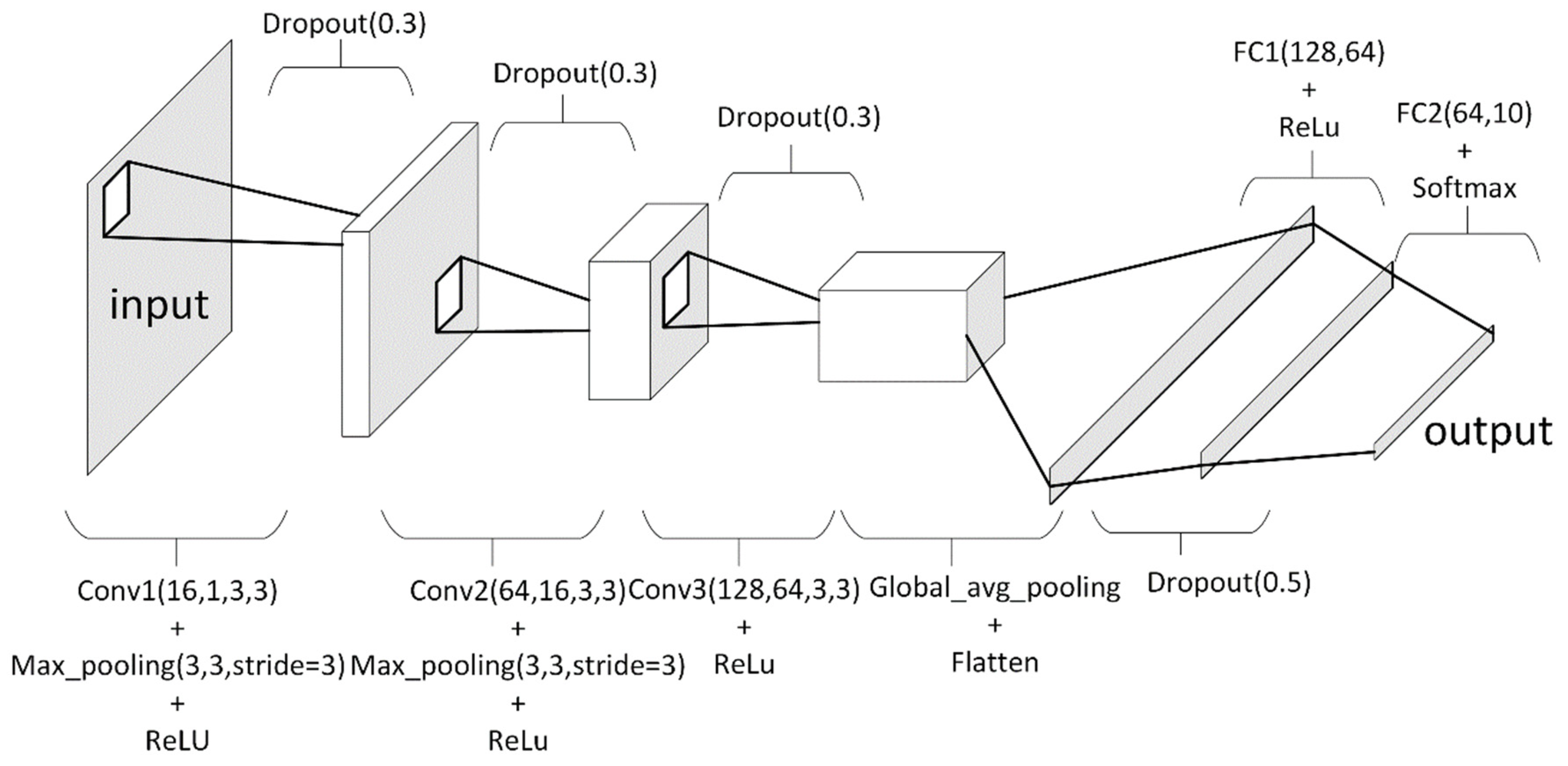
Our network, which can be seen in Figure 1, contains two convolutional layers with max pooling and an additional convolutional layer that precedes a global average pooling layer. We use global average pooling to reduce the needed parameters of the dense layer that follows convolutional layers for two reasons. Firstly, our hardware constraints limited us against larger network models, and secondly, in our research case, implementing an arbitrary network model does not weaken our point of showing the capabilities of fractional-order calculus framework.
Essentially, a deep neural network is a nonlinear mapping function with learnable weights W. Given an input representation X, the neural network maps input to the output as in (12). In classification tasks, the output vector is a vector of class probabilities. In this work, the implemented network has a layer size of 5.
The first three layers are 2D convolutional layers. A convolutional layer can be expressed as in (13).
In this expression, is a pointwise activation function. In our implementation, we use a Rectified Linear Unit (ReLu) activation function for convolutional layers. ReLu expression can be seen in Equation (14).
Additionally, represents convolution operation and W and B are learnable tensors. Bias vector B can be excluded in implementations. 2D convolutional layers consist of N input channels and M output channels. Notationally, when B is excluded, a 2D Convolutional layer can be defined by the shape of tensor W, which has the shape of . is the shape of a convolutional kernel.
Layers 4 and 5 are fully connected layers. As seen in (15), this layer employs a matrix product.
If X is a vector with size N and the output size is M, excluding the bias term B, tensor W can be represented with the shape of (M, N).
For the experiments conducted for this research, the implemented Deep Neural Network resembles the network in [7].
2D Convolutional Layer 1: The number of output channels in this layer is 16. The convolutional kernel has the shape of (3,3). The shape of W in this layer can be given as (16,1,3,3). This convolutional layer is followed by (3,3) strided max pooling layer and ReLu activation.
2D Convolutional Layer 2: The number of input channels in this layer is 16 and the number of output channels is 64. The convolutional kernel has the shape of (3,3). The shape of W in this layer can be given as (64,16,3,3). A (3,3) strided max pooling layer and ReLu activation are applied to the outputs of the 2D convolutional layer.
2D Convolutional Layer 3: The number of input channels in this layer is 64 and the number of output channels is 128. The convolutional kernel has the shape of (3,3). The shape of W in this layer can be given as (128,64,3,3). ReLu activation is applied to the outputs of the 2D convolutional layer. A global average pooling is applied after activation and the outputs are flattened resulting in a vector with a size of 128. This operation is applied to further reduce the parameter size and training time of our network, due to our hardware constraints.
Fully Connected Layer 1: This layer has 64 output units. The shape of W in this layer is (128,64). This layer is followed by ReLu activation.
Fully Connected Layer 2: This layer has 10 output units, which is the same as the number of classes. The shape of W in this layer is (64,10). This layer is followed by Softmax activation to map layer outputs to class probabilities.
Following each layer, Dropout operations with probabilities 0.3 for the first three layers and 0.5 for fully connected layer 1 are applied. The loss function for model optimization is Cross-entropy Loss. For optimization, ADAM optimizer is employed with a learning rate of 0.001, epsilon parameter of , and weight decay parameter of . Weight decay penalizes the squared magnitude of weight values and can be named the L2 regularization. Regularization has been used in deep learning to prevent weight bias and overfitting.
For all experiments, the trainings epoch number is selected as 100. While evaluating the classification performance, a 10-fold cross-validation procedure is applied. The UrbanSound8k dataset was published by its creator as divided into 10 folds. In the 10-fold cross-validation procedure, first, a fold is randomly selected and the network is trained with other folds. The classification accuracy is evaluated on the selected fold. After that, all the network weights and the optimizer is initialized again. These steps are repeated until the classification accuracies for all folds are calculated.
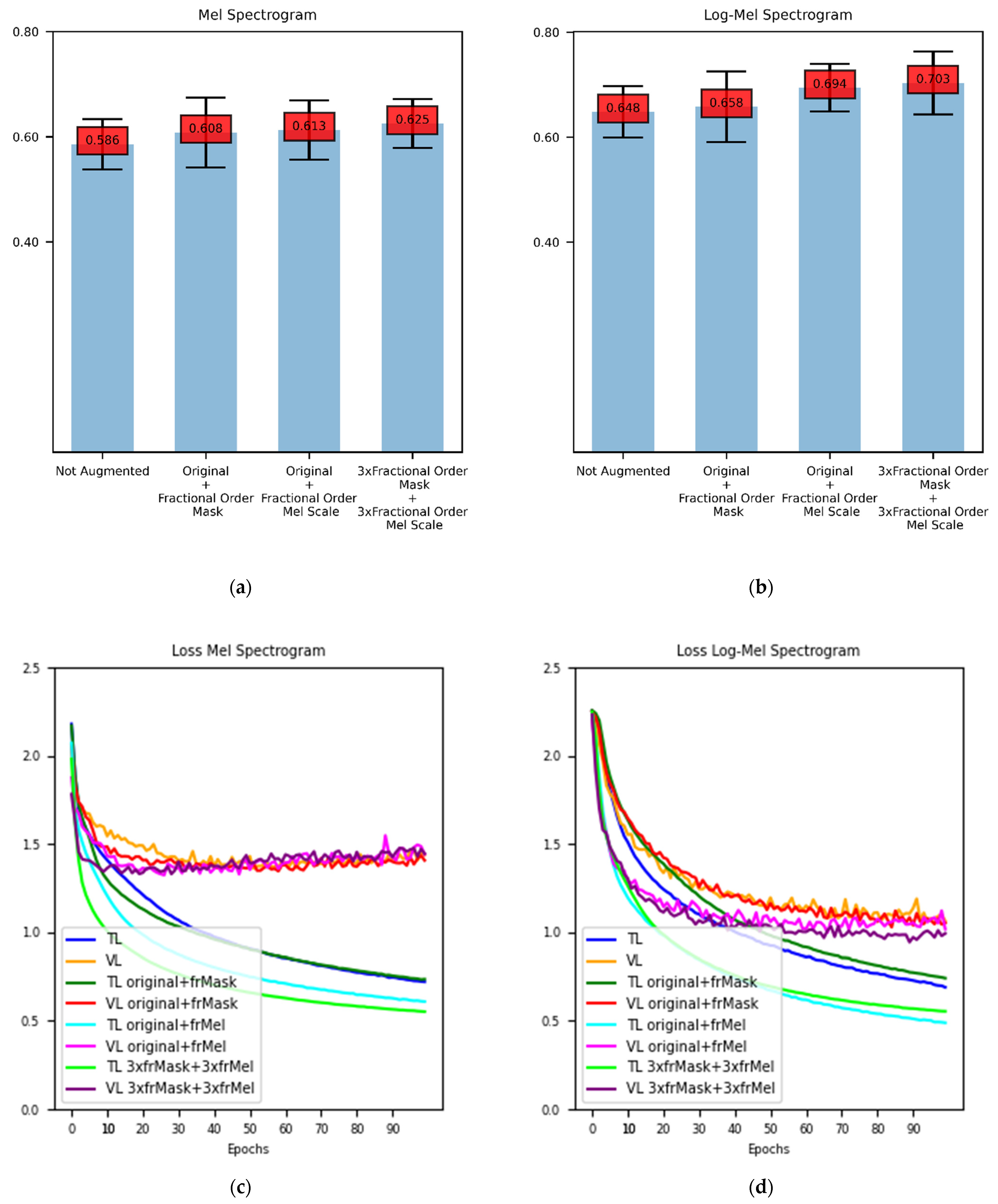
The data augmentation method performances are presented with respect to the mean accuracy. In Figure 2a,b, the results for both Mel spectrogram features and Log-Mel spectrogram features can be seen.
For non-augmented Mel spectrogram features, the accuracy result becomes 58.6%. When we augment the dataset with Fractional-Order Mask and add it to the original dataset, we achieve 60.8% accuracy. When the same procedure is conducted for Fractional-Order Mel-Scale augmentation method, we achieve 61.3% accuracy. When the dataset size is increased by six times with both augmentation methods, the mean accuracy for 10-fold cross-validation becomes 62.5%.
When we change the input features to Log-Mel spectrogram representations, the accuracy result for the non-augmented case is 64.8%. Augmenting the dataset with Fractional-Order Mask and combining the augmented samples with non-augmented log Mel spectrogram features results in 65.8% accuracy, whereas, the same procedure for Fractional-Order Mel-Scale method gives 69.4% accuracy. For the last experiment, the dataset is augmented with both methods separately to increase its size three times. After the augmentation, both augmented datasets are combined. This procedure results in 70.3% accuracy. For Log-Mel spectrogram features, augmenting the dataset six times its original size with fractional-order calculus-based data augmentation methods produces an 8.48% relative increase in accuracy in our experiments.
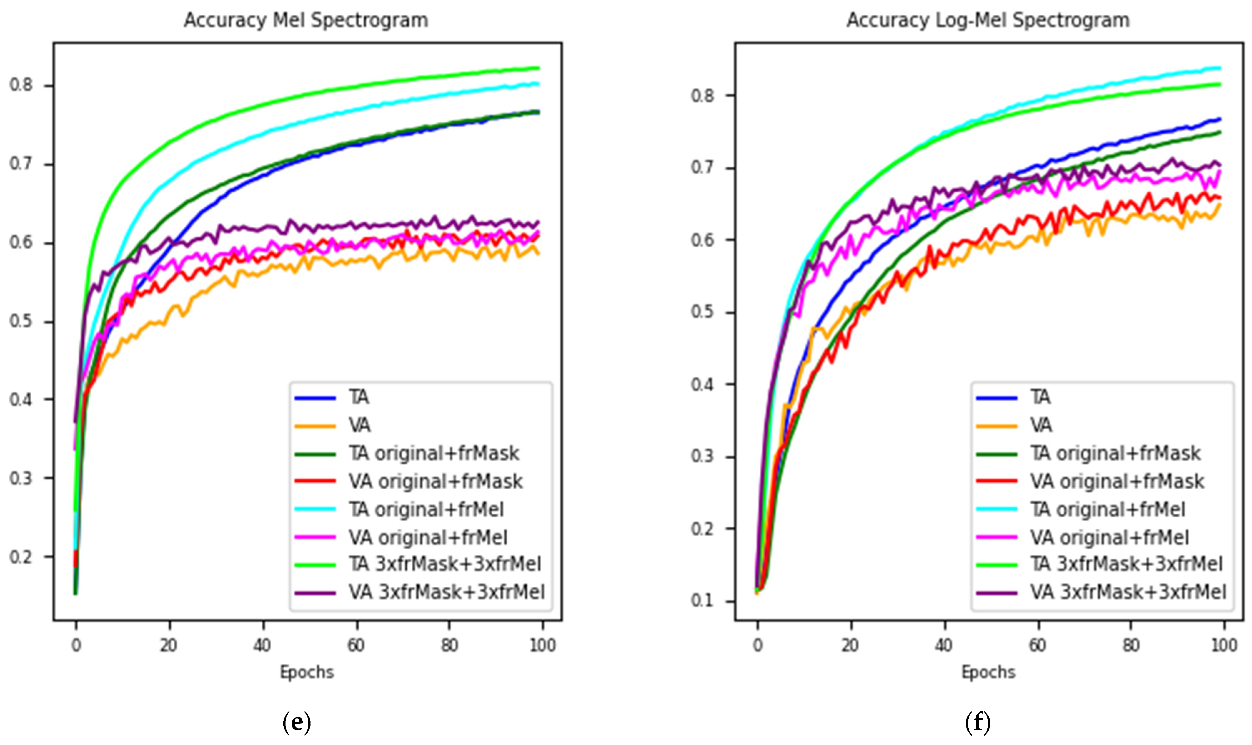
In Figure 2c–f, the loss and accuracy graphs with respect to the epochs are provided. In Figure 2c,d, it is clear that data augmentation reduces the loss both for training and validation data. To achieve saturation, augmented data need fewer epochs. In Figure 2e,f, augmented datasets achieve higher accuracy results both for training and validation. In Figure 2f, augmenting the dataset two times with the Fractional-Order Mel-Scale augmentation method produces higher training accuracy, on the other hand, augmenting the dataset six times with both of the proposed data augmentation methods achieves the highest validation accuracy.
To inspect the results with respect to the increased complexity of the network model, the output unit size of the fully connected layer is increased from 64 to 256. This experiment produces a 66.3% accuracy score for non-augmented Log-Mel spectrogram features. Repeating the procedure with the fully augmented dataset results in 71.4% accuracy.
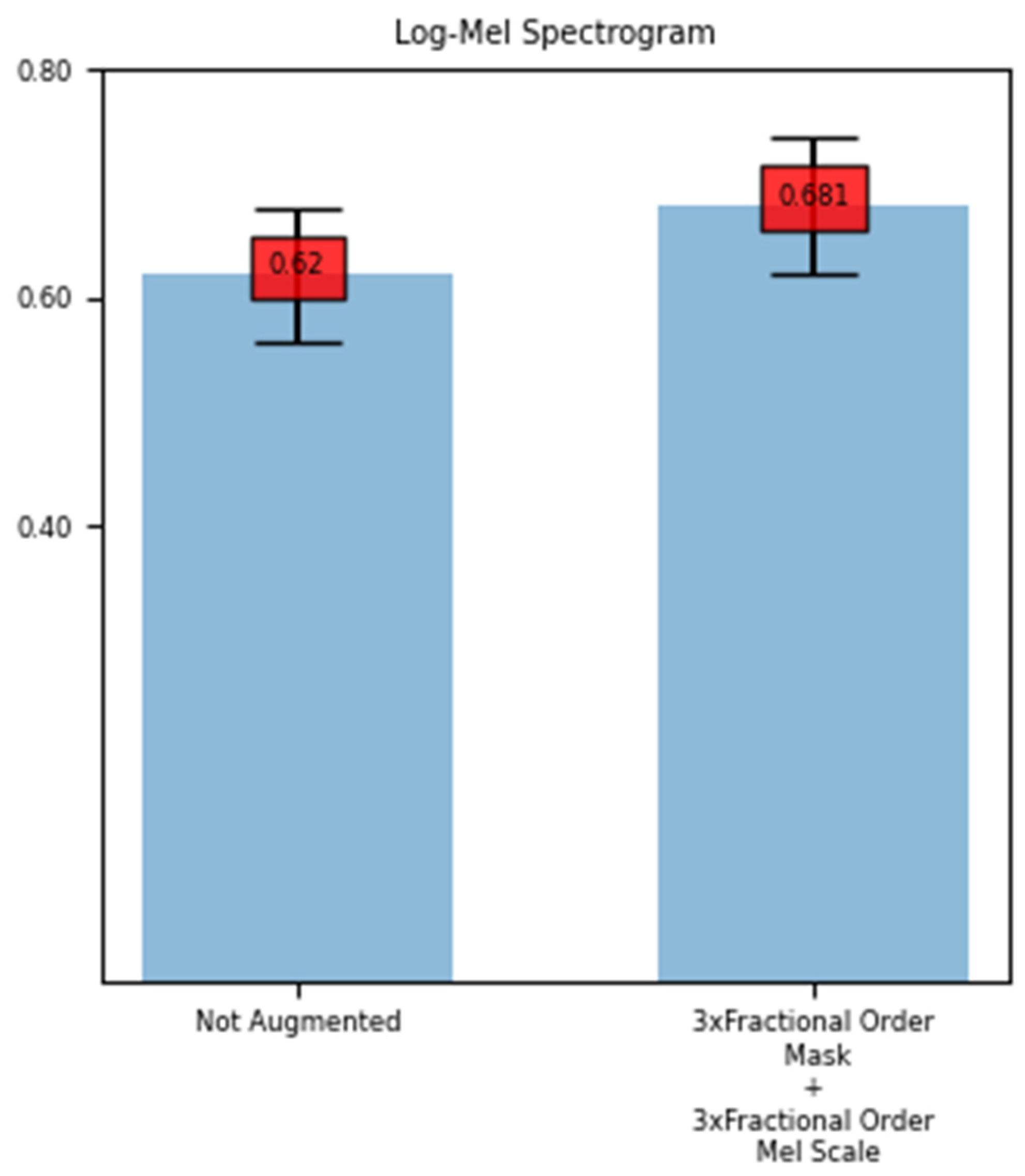
To further understand the performance of data augmentation methods on deeper neural networks an 18-layered ResNet-based model is implemented. The two differences of this implementation are on the input layer and on the output fully connected layer. The network parameters are randomly initialized. The original ResNet model is designed to have three-channel image data as the input, that is why a 2D convolutional layer with the weight shape of (3,1,3,3) is added. The original ResNet-18 implementation of Pytorch has 100 output classes. That is why the last fully connected layer is changed to have 10 output units. This network has a parameter size nearly 100 times the test network used in the experiments before. In deep learning, increased parameter size generally leads a network to overfit. This experiment showed that in terms of loss, the proposed data augmentation methods were unable to overcome the overfitting characteristic of a deeper network like ResNet18. The data augmentation performance on ResNet is presented with respect to the mean accuracy. In Figure 3, the results for Log-Mel Spectrogram features of non-augmented and six times augmented datasets are shown.
In terms of accuracy, the augmented dataset achieved a nearly 10% relative increase in terms of validation accuracy after 25 epochs of training. The non-augmented dataset resulted in 62% validation accuracy, on the other hand, after the dataset was augmented six times using fractional-order calculus-based data augmentation methods, the resulting accuracy became 68.1%.
4. Discussion
Fractional-order calculus provides a capable framework for progressively increasing the number of application domains. In this research, we claim that fractional calculus-based approaches can be successfully applied to yet another domain. To our knowledge, there has not been an implementation of fractional-order calculus-based methods for audio data augmentation. Implementing Fractional-Order Mask and Fractional-Order Mel-Scale augmentation methods has proven to be beneficial.
The Fractional-Order Mel-Scale approach employs fractional differentiation of the Mel scale. It extends the group of frequency warping-based methods for data augmentation. The Fractional-Order Mask approach is an application of similar image edge enhancement methods in the audio data augmentation domain.
Using the Log-Mel spectrogram has been a more preferred way in deep learning because log scaling the Mel spectrogram output creates a dynamic range compression. This process results in a more detailed spectrogram image for the deep learning model to learn. The proposed data augmentation methods work better on the Log-Mel spectrogram representation of audio data. As seen from the experiments, the augmentation procedure for Mel spectrogram features achieves up to 6.6% relative increase, whereas, for Log-Mel spectrogram features the relative increase rate becomes 8.48%. This is an expected result. The Fractional-Order Mel-Scale approach results in amplitude deviations with respect to the original sample. Due to our conservative approach, smaller derivation orders are selected. Without the range compression, the variations on amplitude values of augmented data and original data become less significant, resulting in the model seeing the training data as too similar to the original data. More in-depth analysis showed that augmenting the dataset multiple times creates smaller gains with respect to accuracy and in some cases leads the model to overfit. Due to similar reasons as the Fractional-Order Mel-Scale method, the Fractional-Order Mask method creates greater variations from the original data when applied to the Log-Mel spectrogram features of the audio sample.
The aim of this work is not to overcome benchmark accuracy results of the proposed deep learning models for environmental sound classification tasks. A similar deep CNN model as in the literature is chosen but implemented with further global average pooling operation before fully connected layers. Because of our hardware constraints, a network with a smaller number of learnable parameters is preferred. Since, the main objective is to inspect the performance of the proposed data augmentation methods, choosing to implement a model like ours does not weaken our points. Nevertheless, experiments with increased size of output units for the first fully connected layer are conducted. To inspect the results with respect to the increased complexity of the network model, the output unit size of fully connected layer is increased from 64 to 256. This experiment produces a 66.3% accuracy score for non-augmented Log-Mel spectrogram features. Repeating the procedure with the fully augmented dataset results in 71.4% accuracy. The resulting 7.7% relative increase shows that our points with regards to applying fractional-order calculus-based methods are valid. In addition to the test networks, the ResNet-18 model is implemented to understand the performance of the proposed methods on deeper networks. In this experiment, a fully augmented network achieved a more than 9% relative increase in terms of validation accuracy. On the other hand, inspecting the loss and accuracy curves showed that network performance with respect to the overfitting characteristics is not substantially improved. This result leads us to believe that to achieve substantial improvement in terms of overfitting, the current parameter selection procedure for proposed data augmentation methods is not enough and needs improvement. It must be noted that recent studies on deep learning approaches employ more complex optimization policies to overcome overfitting. In our case, it is a conscious choice to keep the training procedure simpler to be able to see the effects of augmentation methods in a clearer way.
As feature works, these proposed methods can be experimented on for better derivation parameter range selection. It must be noted that these types of experiments should take differences in data types and neural network models into account. Additionally, further experiments can be conducted to understand the effects of fractional-order calculus-based data augmentation methods on speech data. Since automatic speech recognition tasks have great importance, trying to propose a parameter selection procedure for the proposed methods based on the human auditory system can be important. Furthermore, the proposed data augmentation method performances should be evaluated against the conventional data augmentation methods. Lastly, combining the proposed methods with conventional data augmentation methods remains an interesting future research topic for us.
5. Conclusions
In this paper, we proposed two fractional-order calculus-based data augmentation methods for audio signals. One approach is based on fractional differentiation of the Mel scale with a randomly selected derivation order. The second approach employs a fractional-order mask that was created with respect to the randomly selected derivation order. We applied both methods to augment the UrbanSound8K environmental sound dataset. For the classification task, we implemented an arbitrary deep CNN model. We also experimented with a ResNet-based network to understand the capabilities and boundaries of proposed methods. The results were presented with respect to the Mel spectrogram and Log-Mel spectrogram features. A 10-fold cross-validation procedure was applied in our tests to produce the mean accuracy score. Our results showed that the application of fractional-order calculus-based data augmentation methods resulted in a substantial increase in accuracy score. To our knowledge, this paper is the first example of employing fractional-order calculus as an audio data augmentation tool.
Author Contributions
Conceptualization, B.G.Y.; formal analysis, M.K.; funding acquisition, M.K.; methodology, B.G.Y.; software, B.G.Y.; supervision, M.K.; validation, B.G.Y.; writing—original draft, B.G.Y.; writing—review & editing, B.G.Y. and M.K. All authors have read and agreed to the published version of the manuscript.
Funding
This work was supported by the Scientific Research Projects Department of Istanbul Technical University, Project Number: MDK-2020-42479.
Data Availability Statement
Publicly available datasets were analyzed in this study. This data can be found here: https://urbansounddataset.weebly.com/urbansound8k.html (accessed on 1 July 2022).
Conflicts of Interest
The authors declare no conflict of interest. The funders had no role in the design of the study; in the collection, analyses, or interpretation of data; in the writing of the manuscript; or in the decision to publish the results.
References
- Halevy, A.; Norvig, P.; Pereira, F. The Unreasonable Effectiveness of Data. IEEE Intell. Syst. 2009, 24, 8–12. [Google Scholar] [CrossRef]
- Shorten, C.; Khoshgoftaar, T.M. A Survey on Image Data Augmentation for Deep Learning. J. Big Data 2019, 6, 60. [Google Scholar] [CrossRef]
- Perez, L.; Wang, J. The Effectiveness of Data Augmentation in Image Classification Using Deep Learning. arXiv 2017, arXiv:1712.04621. [Google Scholar]
- Taylor, L.; Nitschke, G. Improving Deep Learning with Generic Data Augmentation. In Proceedings of the 2018 IEEE Symposium Series on Computational Intelligence, Bangalore, India, 18–21 November 2018; pp. 1542–1547. [Google Scholar] [CrossRef]
- Ragni, A.; Knill, K.M.; Rath, S.P.; Gales, M.J.F. Data Augmentation for Low Resource Languages. In Proceedings of the Annual Conference of the International Speech Communication Association INTERSPEECH 2014, Singapore, 14–18 September 2014; pp. 810–814. [Google Scholar] [CrossRef]
- Rebai, I.; Benayed, Y.; Mahdi, W.; Lorré, J.P. Improving Speech Recognition Using Data Augmentation and Acoustic Model Fusion. Procedia Comput. Sci. 2017, 112, 316–322. [Google Scholar] [CrossRef]
- Salamon, J.; Bello, J.P. Deep Convolutional Neural Networks and Data Augmentation for Environmental Sound Classification. IEEE Signal Process Lett. 2017, 24, 279–283. [Google Scholar] [CrossRef]
- Park, D.S.; Chan, W.; Zhang, Y.; Chiu, C.C.; Zoph, B.; Cubuk, E.D.; Le, Q.V. Specaugment: A Simple Data Augmentation Method for Automatic Speech Recognition. In Proceedings of the Annual Conference of the International Speech Communication Association INTERSPEECH 2019, Graz, Austria, 15–19 September 2019; pp. 2613–2617. [Google Scholar] [CrossRef]
- Fukuda, T.; Fernandez, R.; Rosenberg, A.; Thomas, S.; Ramabhadran, B.; Sorin, A.; Kurata, G. Data Augmentation Improves Recognition of Foreign Accented Speech. In Proceedings of the Annual Conference of the International Speech Communication Association INTERSPEECH 2018, Hyderabad, India, 2–6 September 2018; pp. 2409–2413. [Google Scholar] [CrossRef]
- Wei, S.; Zou, S.; Liao, F.; Lang, W. A Comparison on Data Augmentation Methods Based on Deep Learning for Audio Classification. J. Phys. Conf. Ser. 2020, 1453, 012085. [Google Scholar] [CrossRef]
- Schlüter, J.; Grill, T. Exploring Data Augmentation for Improved Singing Voice Detection with Neural Networks. In Proceedings of the 16th International Society for Music Information Retrieval Conference ISMIR 2015, Málaga, Spain, 26–30 October 2015; pp. 121–126. [Google Scholar]
- Sakai, A.; Minoda, Y.; Morikawa, K. Data Augmentation Methods for Machine-Learning-Based Classification of Bio-Signals. In Proceedings of the 10th Biomedical Engineering International Conference 2017, Hokkaido, Japan, 31 August–2 September 2017; pp. 1–4. [Google Scholar] [CrossRef]
- Jaitly, N.; Hinton, G.E. Vocal Tract Length Perturbation (VTLP) Improves Speech Recognition. In Proceedings of the 30th International Conference on Machine Learning, Atlanta, GA, USA, 16–21 June 2013; pp. 42–51. [Google Scholar]
- Nanni, L.; Maguolo, G.; Paci, M. Data Augmentation Approaches for Improving Animal Audio Classification. Ecol. Inform. 2020, 57, 101084. [Google Scholar] [CrossRef]
- Nanni, L.; Maguolo, G.; Brahnam, S.; Paci, M. An Ensemble of Convolutional Neural Networks for Audio Classification. Appl. Sci. 2021, 11, 5796. [Google Scholar] [CrossRef]
- Nam, H.; Kim, S.; Park, Y. Filteraugment: An Acoustic Environmental Data Augmentation Method. In Proceedings of the ICASSP 2022-2022 IEEE International Conference on Acoustics, Speech and Signal Processing (ICASSP), Singapore, 23–27 May 2022; pp. 4308–4312. [Google Scholar] [CrossRef]
- Yun, D.; Choi, S.H. Deep Learning-Based Estimation of Reverberant Environment for Audio Data Augmentation. Sensors 2022, 22, 592. [Google Scholar] [CrossRef]
- Ma, F.; Li, Y.; Ni, S.; Huang, S.; Zhang, L. Data Augmentation for Audio–Visual Emotion Recognition with an Efficient Multimodal Conditional GAN. Appl. Sci. 2022, 12, 527. [Google Scholar] [CrossRef]
- Bahmei, B.; Birmingham, E.; Arzanpour, S. CNN-RNN and Data Augmentation Using Deep Convolutional Generative Adversarial Network for Environmental Sound Classification. IEEE Signal Process. Lett. 2022, 29, 682–686. [Google Scholar] [CrossRef]
- Podlubny, I. Fractional Differential Equations: Introduction to Fractional Derivatives, Fractional Differential Equations, to Methods of Their Solution and Some of Their Applications; Academic Press: Cambridge, MA, USA, 1999. [Google Scholar]
- Petráš, I. Fractional-Order Nonlinear Systems; Nonlinear Physical Science; Springer: Berlin/Heidelberg, Germany, 2011. [Google Scholar]
- Ortigueira, M.; Machado, J. Which Derivative? Fractal Fract. 2017, 1, 3. [Google Scholar] [CrossRef]
- Sabanal, S.; Nakagawa, M. The Fractal Properties of Vocal Sounds and Their Application in the Speech Recognition Model. Chaos Solitons Fractals 1996, 7, 1825–1843. [Google Scholar] [CrossRef]
- Al-Akaidi, M. Fractal Speech Processing; Cambridge University Press: Cambridge, UK, 2004. [Google Scholar]
- Lévy-Véhel, J. Fractal Approaches in Signal Processing. Fractals 1995, 3, 755–775. [Google Scholar] [CrossRef]
- Assaleh, K.; Ahmad, W.M. Modeling of Speech Signals Using Fractional Calculus. In Proceedings of the 2007 9th International Symposium on Signal Processing and Its Applications, Sharjah, United Arab Emirates, 12–15 February 2007; IEEE: Piscataway, NJ, USA, 2007; pp. 1–4. [Google Scholar]
- Despotovic, V.; Skovranek, T.; Peric, Z. One-Parameter Fractional Linear Prediction. Comput. Electr. Eng. 2018, 69, 158–170. [Google Scholar] [CrossRef]
- Skovranek, T.; Despotovic, V.; Peric, Z. Optimal Fractional Linear Prediction with Restricted Memory. IEEE Signal Process. Lett. 2019, 26, 760–764. [Google Scholar] [CrossRef]
- Skovranek, T.; Despotovic, V. Audio Signal Processing Using Fractional Linear Prediction. Mathematics 2019, 7, 580. [Google Scholar] [CrossRef]
- Maragos, P.; Young, K.L. Fractal Excitation Signals for CELP Speech Coders. In Proceedings of the International Conference on Acoustics, Speech, and Signal Processing, Albuquerque, NM, USA, 3–6 April 1990; IEEE: Piscataway, NJ, USA, 1990; pp. 669–672. [Google Scholar]
- Maragos, P.; Potamianos, A. Fractal Dimensions of Speech Sounds: Computation and Application to Automatic Speech Recognition. J. Acoust. Soc. Am. 1999, 105, 1925–1932. [Google Scholar] [CrossRef]
- Tamulevicius, G.; Karbauskaite, R.; Dzemyda, G. Speech Emotion Classification Using Fractal Dimension-Based Features. Nonlinear Anal. Model. Control. 2019, 24, 679–695. [Google Scholar] [CrossRef]
- Pitsikalis, V.; Maragos, P. Analysis and Classification of Speech Signals by Generalized Fractal Dimension Features. Speech Commun. 2009, 51, 1206–1223. [Google Scholar] [CrossRef]
- Mathieu, B.; Melchior, P.; Oustaloup, A.; Ceyral, C. Fractional Differentiation for Edge Detection. Signal Process. 2003, 83, 2421–2432. [Google Scholar] [CrossRef]
- Henriques, M.; Valério, D.; Gordo, P.; Melicio, R. Fractional-Order Colour Image Processing. Mathematics 2021, 9, 457. [Google Scholar] [CrossRef]
- Padlia, M.; Sharma, J. Brain Tumor Segmentation from MRI Using Fractional Sobel Mask and Watershed Transform. In Proceedings of the IEEE International Conference on Information, Communication, Instrumentation and Control, ICICIC 2017, Indore, India, 17–19 August 2017; pp. 1–6. [Google Scholar] [CrossRef]
- Alidousti, J. Stability and Bifurcation Analysis for a Fractional Prey–Predator Scavenger Model. Appl. Math. Model. 2020, 81, 342–355. [Google Scholar] [CrossRef]
- Alidousti, J.; Ghafari, E. Dynamic Behavior of a Fractional Order Prey-Predator Model with Group Defense. Chaos Solitons Fractals 2020, 134, 109688. [Google Scholar] [CrossRef]
- Li, P.; Li, Y.; Gao, R.; Xu, C.; Shang, Y. New Exploration on Bifurcation in Fractional-Order Genetic Regulatory Networks Incorporating Both Type Delays; Springer: Berlin/Heidelberg, Germany, 2022; Volume 137. [Google Scholar] [CrossRef]
- Li, P.; Yan, J.; Xu, C.; Shang, Y. Dynamic Analysis and Bifurcation Study on Fractional-Order Tri-Neuron Neural Networks Incorporating Delays. Fractal Fract. 2022, 6, 161. [Google Scholar] [CrossRef]
- Huang, C.; Wang, J.; Chen, X.; Cao, J. Bifurcations in a Fractional-Order BAM Neural Network with Four Different Delays. Neural Netw. 2021, 141, 344–354. [Google Scholar] [CrossRef]
- Huang, C.; Liu, H.; Shi, X.; Chen, X.; Xiao, M.; Wang, Z.; Cao, J. Bifurcations in a Fractional-Order Neural Network with Multiple Leakage Delays. Neural Netw. 2020, 131, 115–126. [Google Scholar] [CrossRef]
- Adams, M. Differint: A Python Package for Numerical Fractional Calculus. arXiv 2019, arXiv:1912.05303. [Google Scholar]
- Oldham, K.B.; Spanier, J. The Fractional Calculus Theory and Applications of Differentiation and Integration to Arbitrary Order, 1st ed.; Academic Press: New York, NY, USA; London, UK, 1974. [Google Scholar] [CrossRef]
- Pu, Y.F.; Zhou, J.L.; Yuan, X. Fractional Differential Mask: A Fractional Differential-Based Approach for Multiscale Texture Enhancement. IEEE Trans. Image Process. 2010, 19, 491–511. [Google Scholar] [CrossRef]
- Chen, M.; Pu, Y.F.; Bai, Y.C. Low-Dose CT Image Denoising Using Residual Convolutional Network with Fractional TV Loss. Neurocomputing 2021, 452, 510–520. [Google Scholar] [CrossRef]
- Umesh, S.; Cohen, L.; Nelson, D. Frequency Warping and the Mel Scale. IEEE Signal Process. Lett. 2002, 9, 104–107. [Google Scholar] [CrossRef]
- Diethelm, K. An Algorithm for the Numerical Solution of Differential Equations of Fractional Order. Electron. Trans. Numer. Anal. 1997, 5, 1–6. [Google Scholar]
- Salamon, J.; Jacoby, C.; Bello, J.P. A Dataset and Taxonomy for Urban Sound Research. In Proceedings of the 2014 ACM International Conference on Multimedia, Orlando, FL, USA, 3–7 November 2014; pp. 1041–1044. [Google Scholar] [CrossRef]
- Piczak, K.J. Environmental Sound Classification with Convolutional Neural Networks. In Proceedings of the 2015 IEEE 25th International Workshop on Machine Learning for Signal Processing (MLSP), Boston, MA, USA, 17–20 September 2015; pp. 1–6. [Google Scholar] [CrossRef]
- Chen, Y.; Guo, Q.; Liang, X.; Wang, J.; Qian, Y. Environmental Sound Classification with Dilated Convolutions. Appl. Acoust. 2019, 148, 123–132. [Google Scholar] [CrossRef]
- Mushtaq, Z.; Su, S.F. Environmental Sound Classification Using a Regularized Deep Convolutional Neural Network with Data Augmentation. Appl. Acoust. 2020, 167, 107389. [Google Scholar] [CrossRef]
Figure 1.
Deep Convolutional Neural Network model for environmental sound classification with fractional-order calculus-based data augmentation experiments.
Figure 1.
Deep Convolutional Neural Network model for environmental sound classification with fractional-order calculus-based data augmentation experiments.

Figure 2.
Accuracy scores and accuracy and loss graphs for experiments: (a) Accuracy scores for Mel spectrogram features; (b) Accuracy scores for log Mel spectrogram features. (c) Loss curve for Mel Spectrogram features; (d) Loss curve for Mel Spectrogram features; (e) Accuracy curve for Mel spectrogram features; (f) Accuracy curve for log Mel spectrogram features.


Figure 3.
Accuracy scores for ResNet-18 experiment.


Table 1.
List of some notations that are used for explaining Mel spectrogram representation and, Grünwald–Letnikow and Riemann–Liouville definitions of fractional derivatives.
Table 1.
List of some notations that are used for explaining Mel spectrogram representation and, Grünwald–Letnikow and Riemann–Liouville definitions of fractional derivatives.
| Notation | Explanation |
|---|---|
| Frequency | |
| Mel Frequency | |
| Higher boundary of triangular filter | |
| Lower boundary of triangular filter | |
| Number triangular filter | |
| Index of the filter in the entire filterbank | |
| Output of the filter m | |
| Frequency magnitude response of the triangular filter | |
| denotes the point FFT magnitude spectrum of the windowed audio sample | |
| the number of time bins | |
| Index of the time bin | |
| Filter coefficients | |
| Derivation order | |
| h | Derivation step; since in the application bin indexes are used, h is taken as unit increments, 1 |
Table 2.
Dataset sizes for each experiment.
| Augmentation Procedure | Dataset Size | Feature |
|---|---|---|
| Not Augmented (Original) | 8732 | Mel Spectrogram |
| Original + Fractional Order Mask | 17,464 | Mel Spectrogram |
| Original + Fractional Order Mel Scale | 17,464 | Mel Spectrogram |
| 3 × Fractional Order Mel Scale + 3 × Fractional Order Mask | 52,392 | Mel Spectrogram |
| Not Augmented (Original) | 8732 | Log Mel Spectrogram |
| Original + Fractional Order Mask | 17,464 | Log Mel Spectrogram |
| Original + Fractional Order Mel Scale | 17,464 | Log Mel Spectrogram |
| 3 × Fractional Order Mel Scale + 3 × Fractional Order Mask | 52,392 | Log Mel Spectrogram |
Publisher’s Note: MDPI stays neutral with regard to jurisdictional claims in published maps and institutional affiliations. |
© 2022 by the authors. Licensee MDPI, Basel, Switzerland. This article is an open access article distributed under the terms and conditions of the Creative Commons Attribution (CC BY) license (https://creativecommons.org/licenses/by/4.0/).
Share and Cite
MDPI and ACS Style
Yazgaç, B.G.; Kırcı, M. Fractional-Order Calculus-Based Data Augmentation Methods for Environmental Sound Classification with Deep Learning. Fractal Fract. 2022, 6, 555. https://doi.org/10.3390/fractalfract6100555
AMA Style
Yazgaç BG, Kırcı M. Fractional-Order Calculus-Based Data Augmentation Methods for Environmental Sound Classification with Deep Learning. Fractal and Fractional. 2022; 6(10):555. https://doi.org/10.3390/fractalfract6100555
Chicago/Turabian StyleYazgaç, Bilgi Görkem, and Mürvet Kırcı. 2022. "Fractional-Order Calculus-Based Data Augmentation Methods for Environmental Sound Classification with Deep Learning" Fractal and Fractional 6, no. 10: 555. https://doi.org/10.3390/fractalfract6100555