Optimal Frequency Control of Multi-Area Hybrid Power System Using New Cascaded TID-PI^λD^μN Controller Incorporating Electric Vehicles

Abstract

Modern structures of electrical power systems are expected to have more domination of renewable energy sources. However, renewable energy-based generation systems suffer from their lack of or reduced rotating masses, which is the main source of power system inertia. Therefore, the frequency of modern power systems represents an important indicator of their proper and safe operation. In addition, the uncertainties and randomness of the renewable energy sources and the load variations can result in frequency undulation problems. In this context, this paper presents an improved cascaded fractional order-based frequency regulation controller for a two-area interconnected power system. The proposed controller uses the cascade structure of the tilt integral derivative (TID) with the fractional order proportional integral derivative with a filter (FOPIDN or PI${}^{\lambda }$D${}^{\mu }$N) controller (namely the cascaded TID-FOPIDN or TID-PI${}^{\lambda }$D${}^{\mu }$N controller). Moreover, an optimized TID control method is presented for the electric vehicles (EVs) to maximize their benefits and contribution to the frequency regulation of power systems. The recent widely employed marine predators optimization algorithm (MPA) is utilized to design the new proposed controllers. The proposed controller and design method are tested and validated at various load and renewable source variations, as is their robustness against parameter uncertainties of power systems. Performance comparisons of the proposed controller with featured frequency regulation controllers in the literature are provided to verify the superiority of the new proposed controller. The obtained results confirm the stable operation and the frequency regulation performance of the new proposed controller with optimized controller parameters and without the need for complex design methods.

1. Introduction

The recent installations and widespread use of various new clean renewable energy sources (RESs) have become more vital solutions to face the climate changes [1]. The RES energy transition has become matter-of-fact in recent years [2]. In this context, the use of power electronic-based converters has been increased to integrate the RESs with the utility grids and/or with the other energy sources. However, the power electronic-based RESs suffer from their reduced power system inertia in comparison with the traditional generation systems without power electronic converters [3]. The resulting RES-based modern power systems have reduced power system inertia, and their values are reduced with increasing penetration levels of RESs in power systems. Thence, the cumulative power systems inertia is considerably reduced due to their lacking of the rotating masses of conventional generation system. This, in turn, leads to deteriorating frequency stability and introduces large spikes of frequency compared with the traditional non-renewable energy sources. Therefore, high penetration levels of RESs in modern electrical power systems have introduced reliability, stability, and security concerns [4,5].

To mitigate the unpredicted perturbations in modern power systems, the control system has to reduce the frequency fluctuations in each area and minimize the tie-line power variations [6]. This action is normally defined as the load frequency control (LFC) of interconnected power systems. The main functionalities of LFC are achieved through using the existing speed governors. However, the speed governors cannot solely achieve precise mitigation of the oscillations of frequency and tie-line power of RES-based modern power systems. The speed governors do not have enough ability to balance the load demand with the power generation. Therefore, proper control methods and improved design schemes are essential for maintaining the steady-state frequency deviations of various areas and their tie-line power deviations at minimized or zero values as much as possible [7].

1.1. Literature Review

In the literature, several studies and proposals of LFC and their design processes have been introduced [8,9]. The robust control theory, the internal model-based controllers, the decentralized control schemes, the sliding mode controllers, the adaptive control systems, the intelligent control systems, and the model predictive controllers have found wide applications in the literature [10,11]. Additionally, the classical integer order control methods have shown good performance with disturbance rejection capabilities [12]. Furthermore, the fuzzy logic-based control methods have been integrated with various control methods to adapt and enhance the performance of the LFC at various operating conditions and disturbances [13]. In addition, recent deep learning and data-driven LFC schemes have been presented to solve the frequency regulation problems [14,15]. However, they need huge training data to optimize their performance.

From another point of view, the fractional order (FO) LFC schemes have found wide applications in frequency regulation in single- and multi-area power systems [16]. They have shown better performance than the traditional integer order-based LFC schemes. Moreover, they add more flexibility and degree of freedom to the design process of LFC systems due to the extra added tunable parameters of the fractional order operators. The FO-based LFC represent the more general form of integer order-based LFC; they have more freedom to adjust the FO operators of tilt, integer, and differential terms. The FO-based proportional-integral-derivative (PID) (namely FOPID) LFC has been presented in the literature to improve the performance of the integer order PID method [17]. The comparison has proved to demonstrate a better response to transients with damping oscillations and reduces peak overshoot/undershot values. Moreover, faster steady-state restoration with reduced steady-state error has been obtained using an FO controller compared to the studied integer order controllers. In [18], the FOPID control method was presented and optimally designed using the movable damped-wave optimization algorithm (MDWA) for a multi-area interconnected power system. The high-order differential feedback control method (HODFC) was introduced in [19] for LFC in two-area interconnected power systems. The particle swarm optimization (PSO) algorithm has been utilized for the optimum tuning of the gains of the HODFC. The optimization of the FOPID was proposed using the sine-cosine optimizer algorithm (SCA) in [20]. However, the presented controller cannot achieve damping out of wide ranges of the fluctuations owing to the use of a single degree of freedom.

The tilt-integral-derivative (TID)-based LFC has been widely introduced in the literature. The TID LFC methods possess improved feedback due to their transfer function, which is very close to the optimum [21]. In [22], a TID-based LFC was presented with a high-pass filter to reduce existing input noise effects on the system stability. Another application of TID LFC was presented in [23], and it was optimized using the artificial bee-colony optimizer algorithm (ABC). Another LFC method based on the TID control method was introduced in [24]. The optimization process was made using the pathfinder optimization algorithm (PFA). The differential evolution optimizer algorithm (DE) was introduced in [22] for optimizing the TID control with a filter for LFC methods. A combined PI and TD with a filter controller was proposed in [25] with the slap swarm optimization algorithm (SSA). A parallel combination of TID with a filter and TID was proposed in [26], and a hybrid algorithm of a modified particle swarm optimizer with the genetic algorithm (MPSOGA) was presented for designing the controller.

Additionally, combined and hybrid FO-based LFC methods have been presented in the literature. A hybrid FO controller was proposed in [21] for gate-controlled series-capacitor (GCSC)-based interconnected power systems. Another hybrid FO LFC was proposed in [27] for superconducting energy storage system (SMES)-based interconnected two-area power systems. A parallel combination of the hybrid FO LFC with the TID with a filter was presented in [28] with an optimum design of the presented controller. A modified hybrid decentralized FO-based LFC and EV controller was presented in [29]. The presented LFC and EV controllers combine the FOPID and TID controllers. Moreover, the artificial ecosystem optimizer (AEO) algorithm was presented to optimize the presented controller parameters.

Moreover, fuzzy logic is integrated in the literature with the FO-based LFC to combine both features. Fuzzy-FOPI was proposed in [30]. Additionally, fuzzy-FOPID with a filter was introduced in [31]. In [32], the cascaded fuzzy LFC method was proposed, with an ICA optimizer for multi-area power systems. A combined fuzzy logic and FOPID LFC method was presented in [33]. A cascaded fuzzy method with FOPID was presented in [34] with the water cycle optimization algorithm (WCA). In [35], fuzzy logic with PID with a filter and FOPI controllers has been presented. The optimization of the presented controller has been made through the imperialist competition optimization algorithm (ICA).

It can be seen that further development and advanced LFC schemes are needed to improve the frequency regulation of multi-area interconnected power systems. Additionally, the associated problems of high penetration levels of RESs in modern power systems with the uncertainties in the model parameters of electrical power systems represent another challenges for existing controllers and/or design methods.

1.2. Paper Contribution

Based on the motivation by the existing gap in LFCs and their design methods, the main contributions of this paper are summarized as follows:

• An improved cascaded fractional order based load frequency control method is proposed for the two-area interconnected power system. The proposed controller uses the cascade structure of the tilt-integral-derivative (TID) with the fractional order proportional-integral-derivative with filter (FOPID or PI${}^{\lambda }$D${}^{\mu }$N) controller (Cascaded TID-FOPIDN or TID-PI${}^{\lambda }$D${}^{\mu }$N controller). Based on the authors’ knowledge, this is the first time that a cascaded TID-FOPIDN control structure has been proposed for LFC in interconnected power systems.
• Compared to existing LFC systems and existing cascaded LFC structures, the proposed controller is advantageous at mitigating the frequency and tie-line power fluctuations in comparison to the studied LFC from the literature. Comparisons are provided to verify the superiority of the proposed controller over the existing featured FO LFC methods. Moreover, various performance metrics are compared with the featured cascaded control structure in the literature for the various considered scenarios.
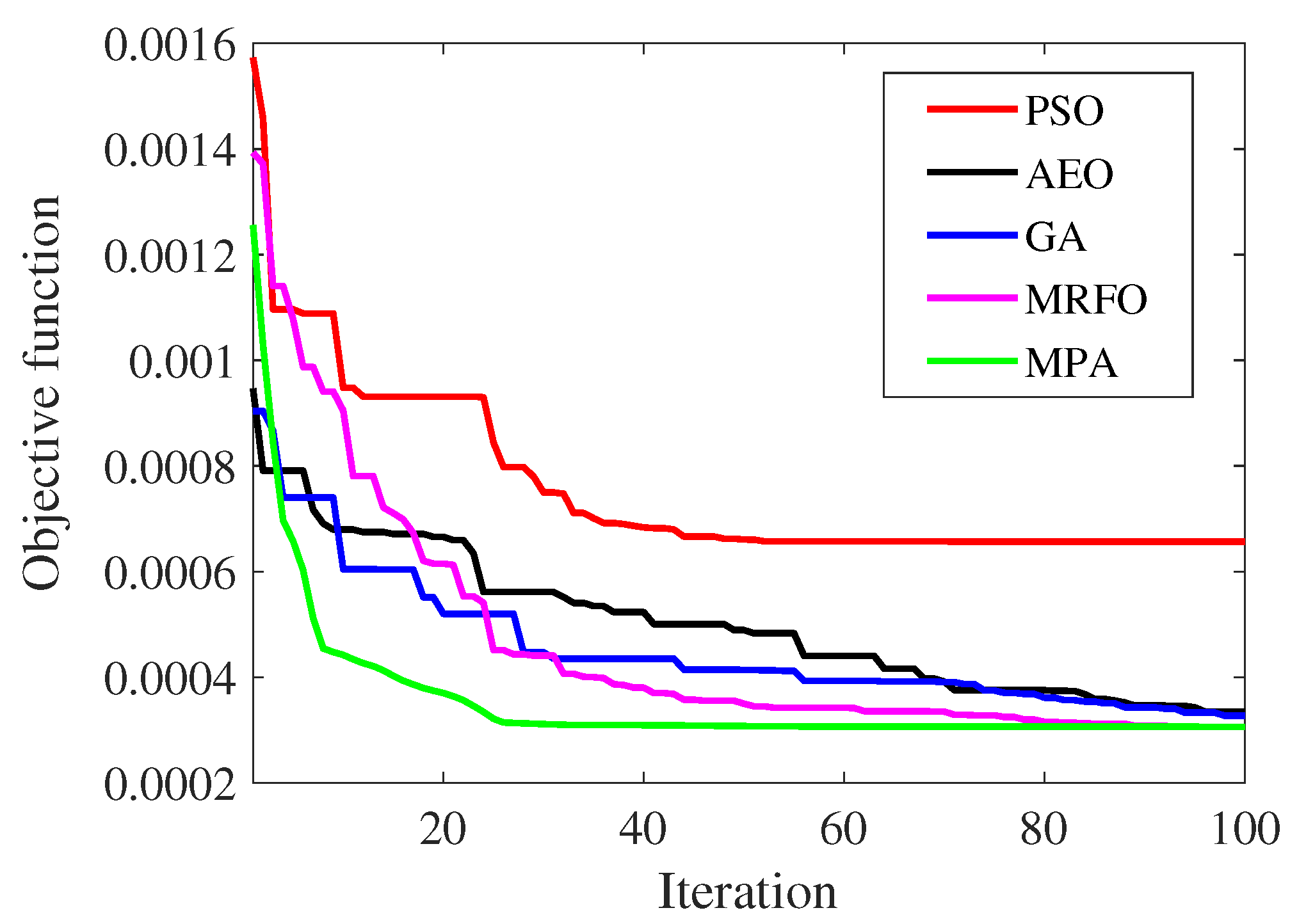
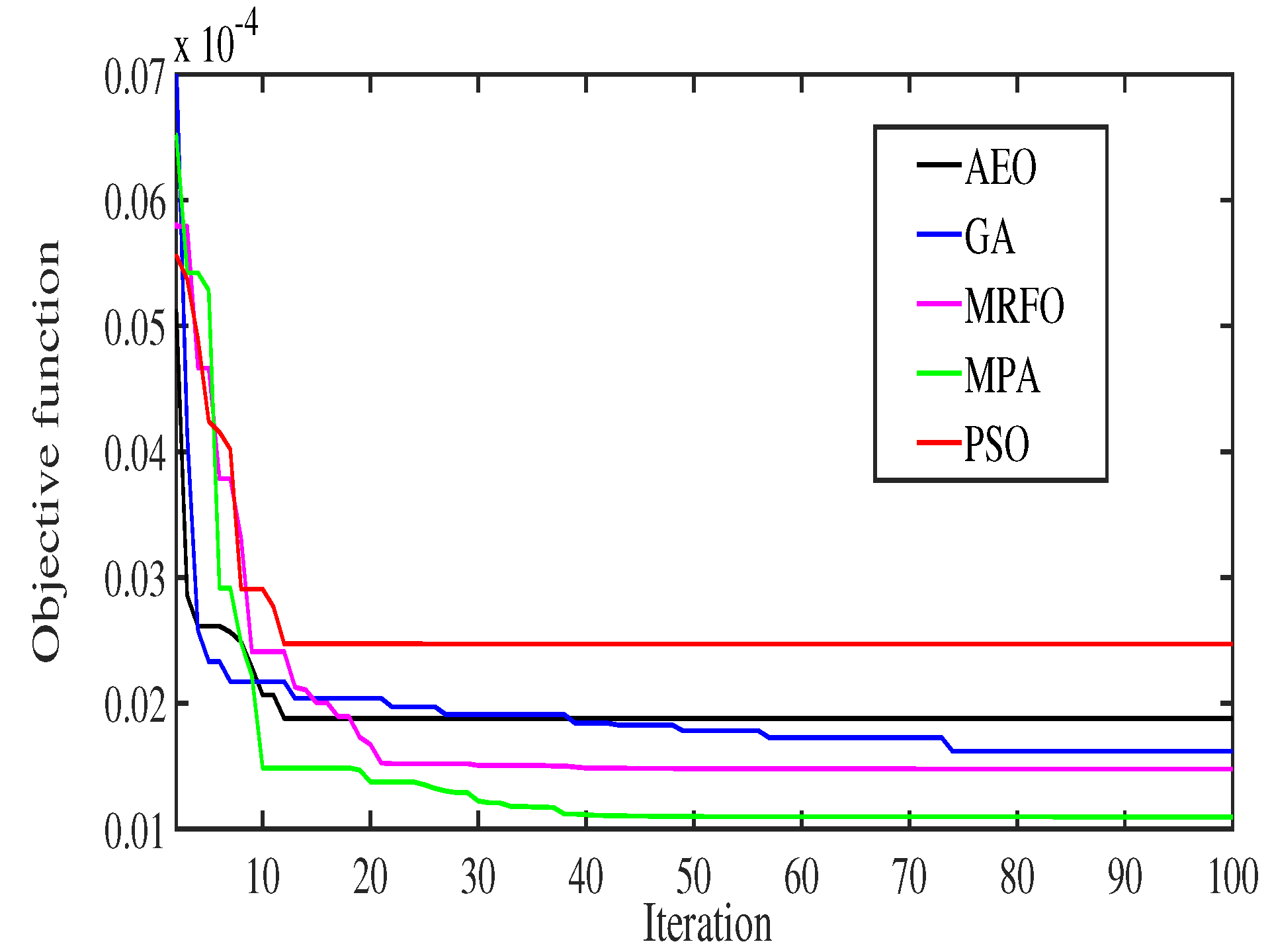
• The performance of the proposed LFC method is enhanced using the marine predators optimization algorithm (MPA) to optimally determine the parameters of the proposed controller. Additionally, the MPA performance is verified through comparisons with the other existing algorithms.
• A cooperative control of the connected electric vehicles (EVs) based on TID fractional order control is also proposed in this paper. The proposed controller is capable of effectively participateing in regulating the frequency of the interconnected power systems.
• The proposed LFC and EV control system are also integrated with the stochastic conditions and characteristics of renewable energy sources to demonstrate the robustness and superiority of the proposed work.

The remaining parts of the paper are organized as follows: the modeling of the selected multi-source multi-area power systems is presented in Section 2. Section 3 presents the new proposed cascaded TID-FOPIDN controller and the control design methodology. The simulation results and the performance comparison are detailed in Section 4. The conclusion of the paper is made in Section 5.

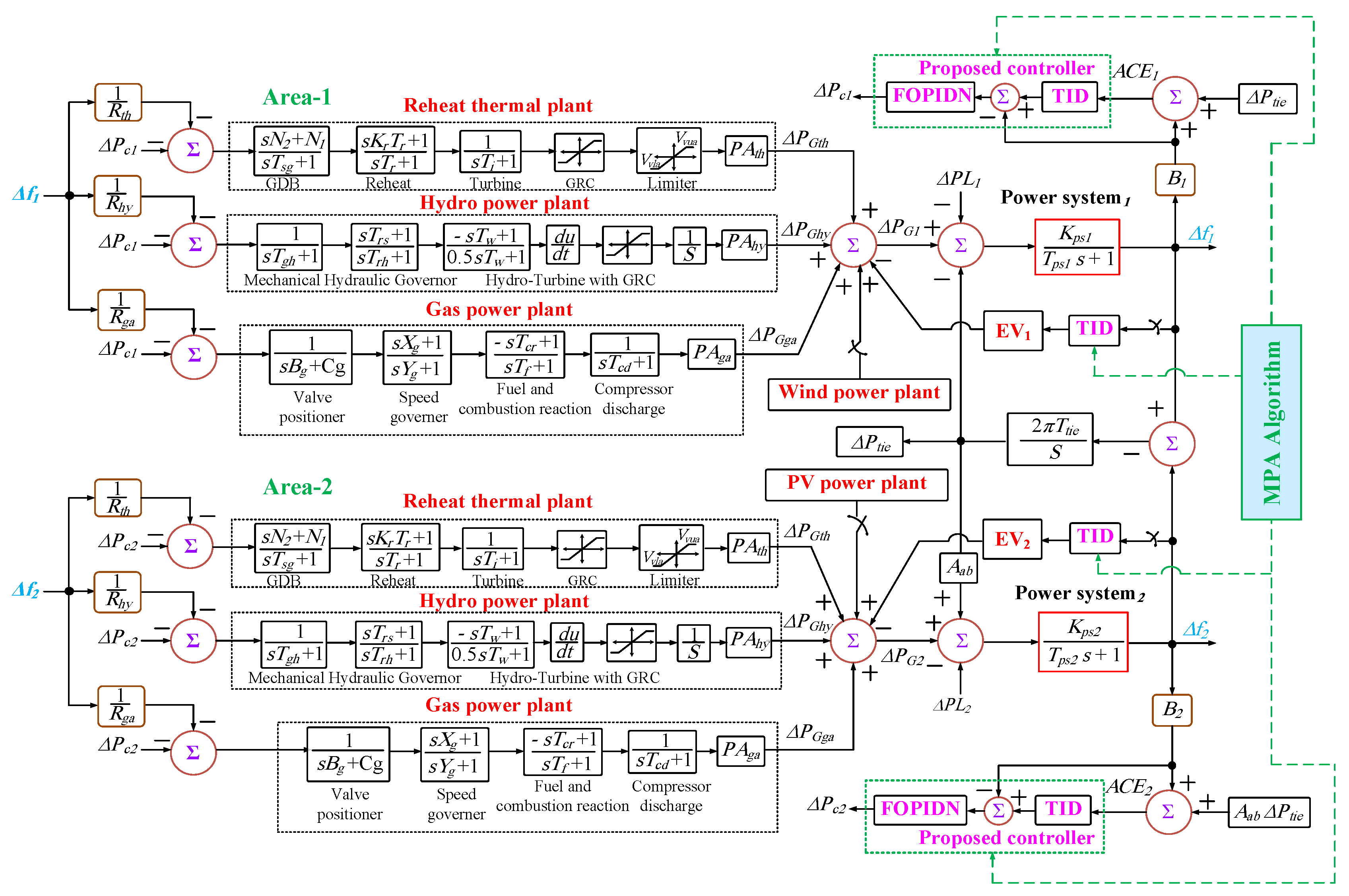
2. Models of Various Elements in the Multi-Source Power System

2.1. The Case Study

The selected case study includes two interconnected power systems with multiple sources in each area, including a reheating thermal plant, hydro power plant, and gas plant. The participation of an EV is considered in both areas to regulate the frequency. Aldditionally, renewable energy is considered in both areas with their dependence on the ambient conditions of solar irradiance, wind speed, and temperature. The variations of electric loads is considered as a disturbance in each area. The representation of various elements in both areas is detailed in Figure 1. It can be seen that there are models of the three generating plants in each area. Additionally, each area has its frequency controller to control the power generation of different units. Another controller is added in each area to control the injected power from EVs and to participate in the frequency regulation in each area.

Table 1. System data of various power system elements for the case study.

Acronyms	Study Factors
	Area 1	Area 2
LFC model
$R_{th}$,$R_{hy}$,$R_{ga}$ (Hz/MW)	2.4	2.4
$B_1$,$B_2$ (MW/Hz)	0.4312	0.4312
Power system
$P_{r1}$,$P_{r2}$ (MW)	2000	2000
$\Delta P_L$ (MW)	1740	1740
$K_{ps1}$,$K_{ps2}$	68.9655	68.9655
$T_{ps1}$,$T_{ps2}$	11.49	11.49
$T_{tie}$	0.0433
$A_{ab}$	−1
Reheating thermal plant
$\Delta P_{Gth}$ (MW)	946	946
$T_{sg}$	0.08	0.08
$T_t$	0.3	0.3
$K_r$	0.3	0.3
$T_r$	10	10
$P{A}_{th}$	0.54367	0.54367
Hydro power plant
$\Delta P_{Ghy}$ (MW)	567	567
$T_{gh}$	0.2	0.2
$T_{rh}$	28.749	28.749
$T_{rs}$	5	5
$T_w$	1	1
$P{A}_{hy}$	0.32586	0.32586
Gas unit
$\Delta P_{Gga}$ (MW)	227	227
$B_g$	0.049	0.049
$C_g$	1	1
$X_g$	0.6	0.6
$Y_g$	1.1	1.1
$T_{cr}$	0.01	0.01
$T_f$	0.239	0.239
$T_{cd}$	0.2	0.2
$P{A}_{ga}$	0.130459	0.130459

and

Table 2. RESs and EV for the case study.

Acronyms	Study Factors
	Area 1	Area 2
PV power plant
$T_{PV}$ (s)	-	1.3
$K_{PV}$ (s)	-	1
Wind power plant
$T_{WT}$ (s)	1.5	-
$K_{WT}$ (s)	1	-
EV model
Penetration Level	5–10%	5–10%
$V_{nom}$ (V)	364.8	364.8
$C_{nom}$ (Ah)	66.2	66.2
$R_s$ (ohms)	0.074	0.074
$R_t$ (ohms)	0.047	0.047
$C_t$ (farad)	703.6	703.6
$RT/F$	0.02612	0.02612
Maximum $SOC$%	95	95
$C_{batt}$(kWh)	24.15	24.15

summarize the different model parameters of the existing elements in each area as in [36,37,38].

The nonlinearities of components represent an important factor in designing and testing the effectiveness of the proposed controllers. The physical constraints of generating stations are taken into consideration in the studied system, including the generation rate constraint (GRC) and governor dead band (GDB) of the thermal units, with the GRC for increasing and decreasing rates set at 10% pu/min (0.0017 pu.MW/s). Additionally, the GRC constraints are considered for the hydro power plant with increasing and decreasing rates is 270 percent pu/min (0.045 pu.MW/s) and 360 percent pu/min (0.06 pu.MW/s), respectively. A linearized version of the GDB can be used in terms of the change and the rate of change in speed [36]. Based on Fourier series, the transfer function model of GDB with 0.5 percent backlash is obtained as follows:

$$\begin{array}{c}\mathrm{G}\mathrm{D}\mathrm{B}=\frac{s{N}_2+N_1}{s{T}_{sg}+1}\hfill \end{array}$$

(1)

where $N_1$ and $N_2$ are the Fourier coefficients, and they are selected as $N_1$ = 0.8 and $N_2$ = −0.2/$\pi$ based on the data in [36,38].

2.2. The PV Plant Model

With the output characterstics of solar PV panels, and with the necessity to continuously track the operating maximum power point, power electronics interfaces have become essential parts in the grid integration of solar PV systems. The power electronic inverters and the AC power system synchronization interconnection is widely used in solar PV plants with different topologies and connections. Moreover, the weather conditions possess great influences on the PV system outputs, which makes the output power of solar PV systems unpredictable. Thence, the high-frequency changes due to the PV solar output power result in stability problems of solar PV systems. The model of the output power from the solar PV system can be presented as the following [39,40]:

$$P_{\mathrm{P}\mathrm{V}}=\eta {\Phi }_{solar}S[1-0.005(T_a+25)]$$

(2)

where $\eta$ is the conversion efficiency of PV panel (in %), ${\Phi }_{solar}$ is the solar insolation ($\mathrm{W}/{\mathrm{m}}^2$), S is the PV unit’s area (${\mathrm{m}}^2$), and $T_a$ is the ambient temperature ($°\mathrm{C}$). The configuration model of a realistic PV solar generation system is implemented using the model in [41].

2.3. The Wind Turbine Model

The mechanical power output of a wide turbine generation (WTG) system is highly fluctuating due to the intermittent nature of tje wind speed. It can be evaluated as follows [39,40]:

$$P_{wind}=\frac{1}{2}\rho A_r{C}_p{V}_w^3$$

(3)

where $\rho$ is the air density in kg/m${}^3$, $A_r$ is the swept area in m${}^2$, $C_p$ is the power coefficient, and $V_w$ is the wind speed in m/s. The configuration model of a realistic WTG system is implemented using the model in [41].

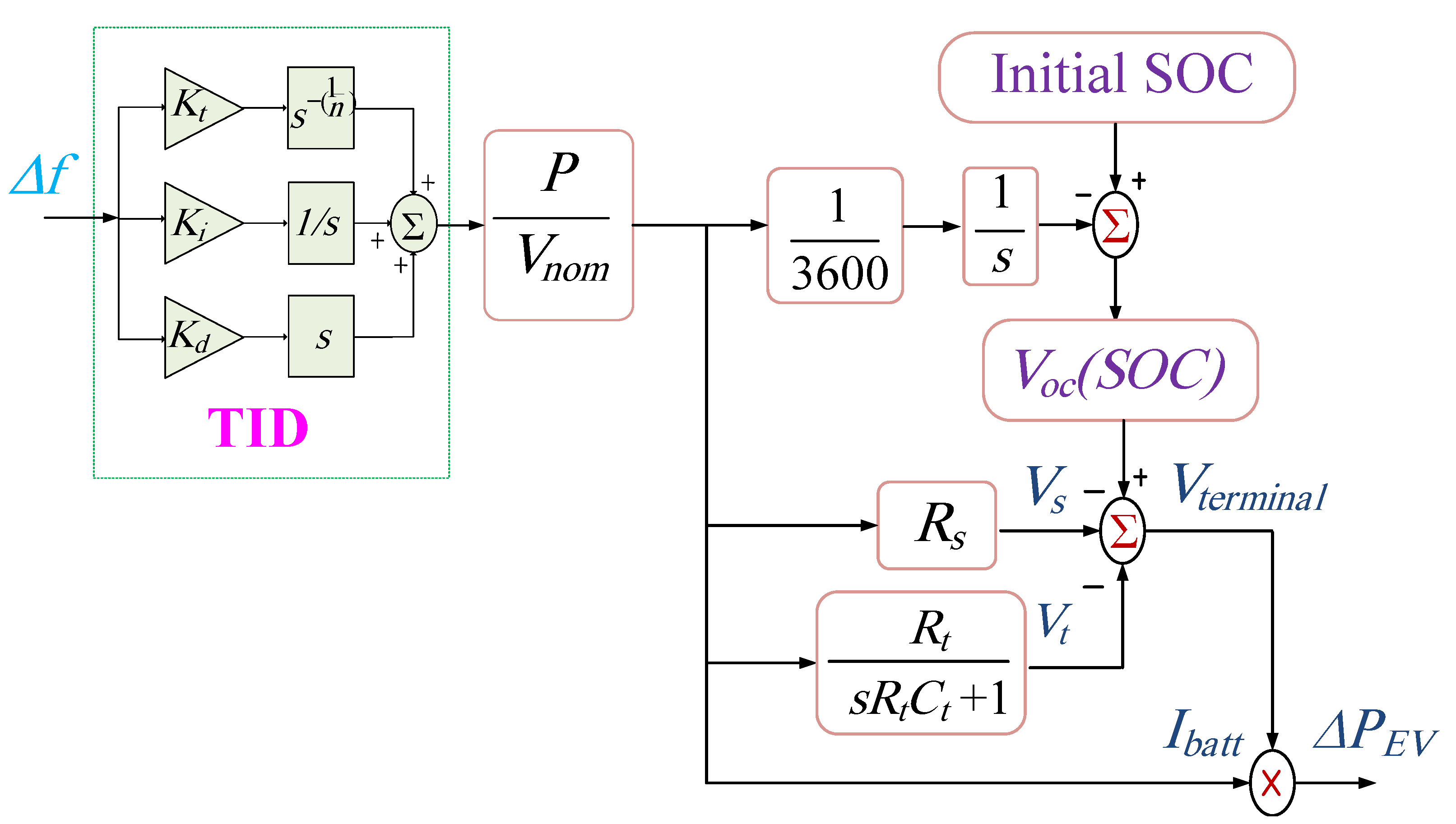
2.4. The Model of EV Systems

The batteries of existing EVs can participate effectively in regulating the power system performance. They can charge/discharge based on the requirements of the electrical power system management. They can lead to the improvement of power system performance, including improving the dynamic response, efficiency, and reliability. The participation of an EV in preserving a power system’s frequency stability due to the fluctuating nature of RESs and the connected electrical loads represents an important task of their use. Figure 2 presents the dynamical model of EV systems for frequency response analysis as modelled in this paper [29]. In the model, the Nernst equation is employed for representing the relationship between the open circuit voltage ($V_{oc}$) and the state of charge ($SOC$) of the connected EVs [29]:

$$V_{oc}\left(SOC\right)=V_{nom}+S\frac{RT}{F}ln\left(\frac{SOC}{C_{nom}-SOC}\right)$$

(4)

where $V_{oc}\left(SOC\right)$ represents the $V_{oc}$ as a function of their $SOC$, $V_{nom}$ denotes the nominal voltage, and $C_{nom}$ denotes the nominal capacities of EV batteries (in Ah). Furthermore, S represents the sensitivity parameter between $V_{oc}$ and $SOC$ of the EV batteries. R, F, and T, on the other hand, stand for the gas constant, Faraday constant, and temperature, respectively.

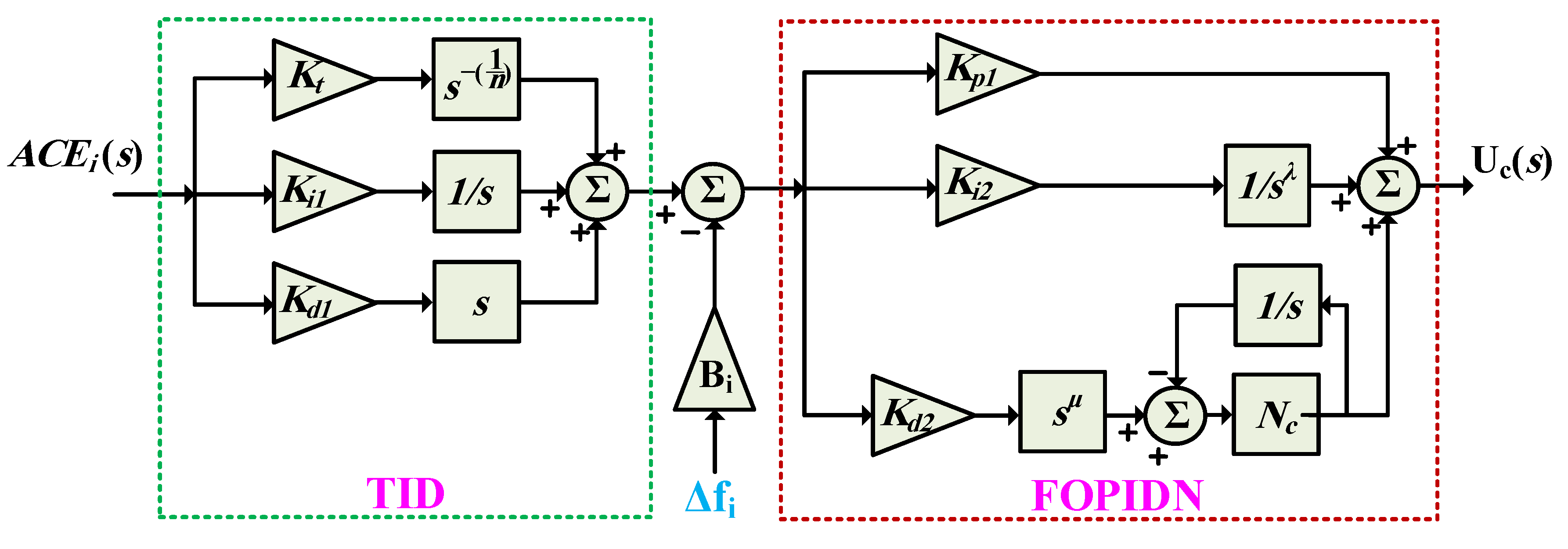
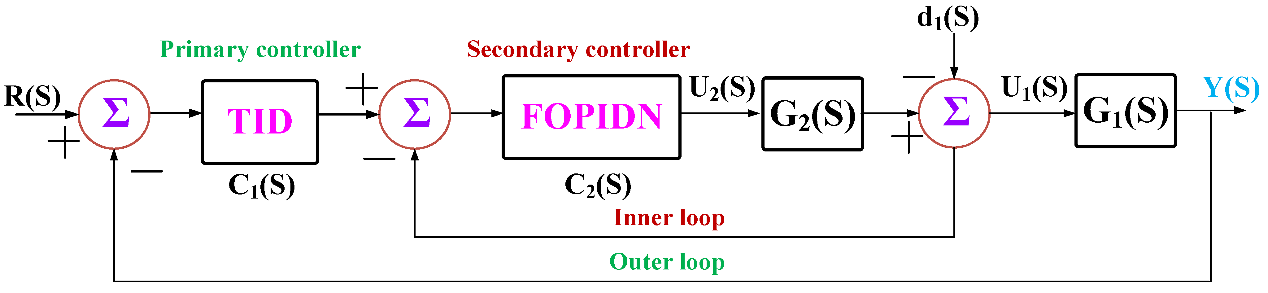
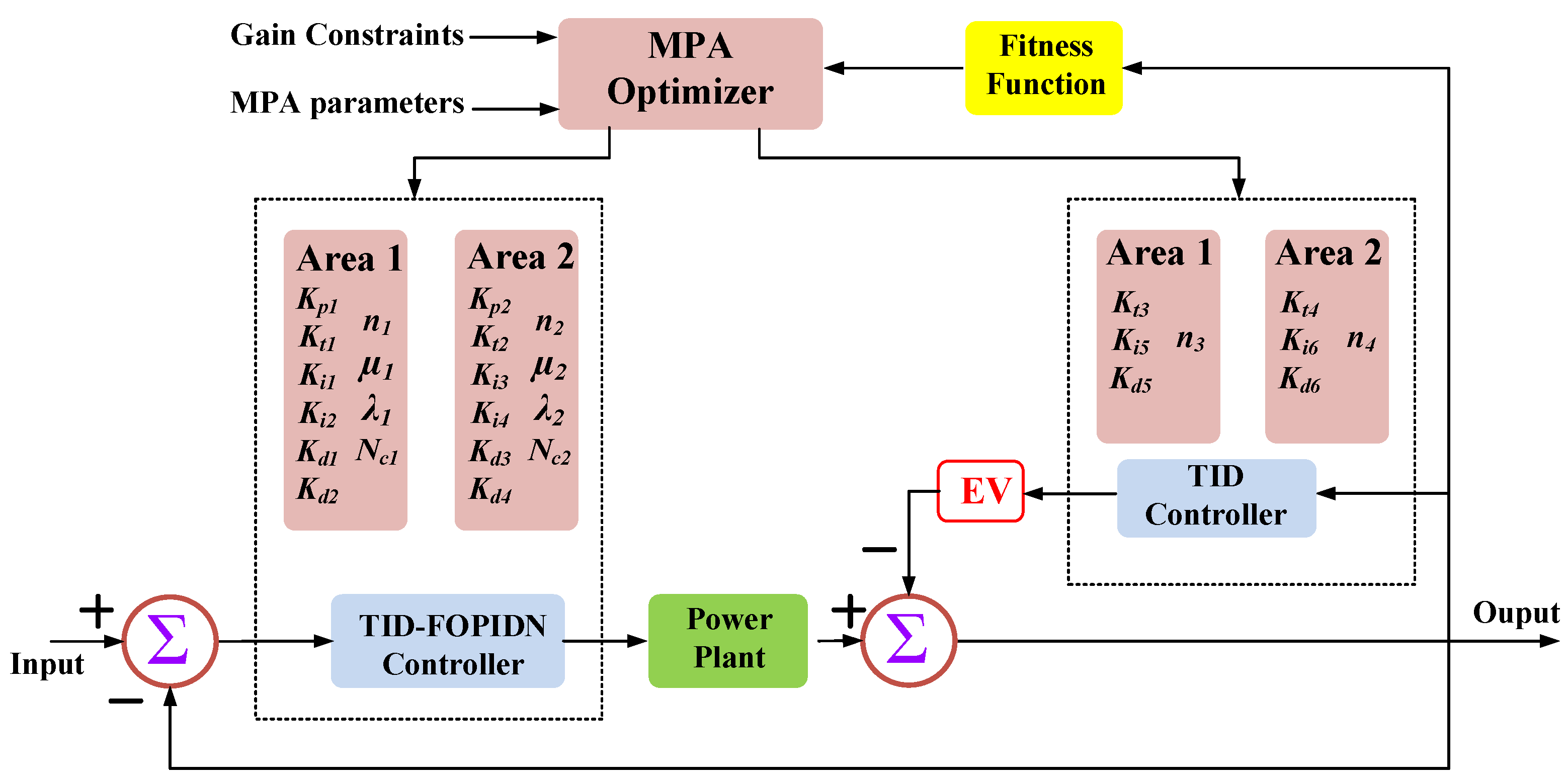
3. The Proposed Optimized Controller

3.1. Overview of Existing Controllers

In literature, several control methods have been proposed for achieving an LFC with various structures and applications. The PID integer order LFC has found wide utilization in frequency regulation. The PID control structure can be represented as follows:

$$C\left(s\right)=\frac{Y\left(s\right)}{R\left(s\right)}=K_p+\frac{K_i}{s}+K_{d}s$$

(5)

It can be seen that an optimum design is needed for the three gains, $K_p$, $K_i$, and $K_d$, which denote the proportional, the integral, and the derivative gains. From another prspective, the FOPID control has been proposed in the literature to merge the advantages of the PID and the FO control structure. The FOPID can be modelled as follows:

$$C\left(s\right)=\frac{Y\left(s\right)}{R\left(s\right)}=K_p+\frac{K_i}{s^{\lambda }}+K_d{s}^{\mu }$$

(6)

where $\lambda$ represents the order of the integral part and $\mu$ represents the order of the derivative part. The tuning of $\lambda$ and $\mu$ is made in their limit range of [0, 1]. The addition of the order $\lambda$ and $\mu$ to the classical PID control leads to improving the dynamical response of the LFC, as proven in the literature [27]. Furthermore, the TID has proven enhanced performance in several applications as an extension for the FOPID control. The TID is expressed as follows:

$$C_1\left(s\right)=\frac{Y\left(s\right)}{R\left(s\right)}=K_t{s}^{-\left(\frac{1}{n}\right)}+\frac{K_i}{s}+K_{d}s$$

(7)

where $K_t$ denotes the tilt gain, and n denotes a non-zero real number. It is usually tuned in the range between 2 and 5 [22,42]. The tuning of various gains and fractional order parts are used in the optimization process of the LFC’s performance.

3.2. The Proposed TID-FOPIDN Controller

The traditional PID control can achieve improved stability and faster response of the controller. However, it suffers from unreasonable injected large control inputs to the plant due to the derivative mode. The main cause of this problem is the existing noise in the control signals. The addition of a filtering part to the derivative part leads to the elimination of the injected noise. Fine-tuning the pole helps to reduce the noise chattering [43].

Therefore, the FOPIDN is selected in the proposed cascaded controller. It includes the FOPID and the derivative filter to improve the control performance. The transfer function of FOPIDN can be represented as follows [16,43]:

$$C_2\left(s\right)=\frac{Y\left(s\right)}{R\left(s\right)}=K_p+\frac{K_i}{s^{\lambda }}+K_d{s}^{\mu }\frac{N_{c}s}{N_c+s}$$

(8)

The structure of the proposed TID-FOPIDN LFC method is represented in Figure 3. The cascaded TID-FOPIDN is employed in both areas, while an additional TID controller is proposed for controlling the existing EVs in each area. The main goal of the designed controller is to regulate the frequency response in each area during load transients, RES variations, and power system uncertainty. The proposed cascaded structure of LFC is advantageous at limiting the disturbance effects that enter the secondary loop from the primary loop. Thence, it can provide better performance compared with single control loop structures. An additional advantage is that they can reduce the impacts of the gain variations on system performance [44].

The employed cascaded control structure uses the output of one control as an input set point for the other control. The TID is employed as the primary outer control loop, or the master controller, and it is responsible for providing the set point for the second stage. The FOPIDN is used for the inner control loop, namely the secondary controller of the slave controller. The structure of the proposed cascaded TID-FOPIDN controller is shown in Figure 3.

Figure 4 shows the control block diagram of the proposed cascaded TID-FOPIDN LFC method. The effects of the disturbances $d_1\left(s\right)$ on the control are reduced due to the cascade control structure. The representation of the transfer function for the inner control loop is as follows [44]:

$$Y_2\left(s\right)=G_2\left(s\right)U_2\left(s\right)$$

(9)

where $G_2\left(s\right)$ denotes the inner process, and $U_2\left(s\right)$ denotes the input signal for $G_2\left(s\right)$. The frequency in each area and the tie-line power are regulated by the outer primary control loop through minimising each area control error. The outer loop control transfer function can be represented as follows [44]:

$$Y\left(s\right)=G_1\left(s\right)U_1\left(s\right)+d_1\left(s\right)$$

(10)

where $G_1\left(s\right)$ denotes the outer process, and $U_1\left(s\right)$ denotes the input signal for $G_1\left(s\right)$.

In the proposed cascaded TID-FOPIDN LFC method, the FOPIDN is represented by the transfer function $C_2\left(s\right)$ for the inner secondary control loop. The transfer function $C_1\left(s\right)$ represents the TID in the outer primary control loop. The ACE signals $AC{E}_1$ and $AC{E}_2$ for area a and area b, respectively, are represented as follows [29]:

$$AC{E}_1=\Delta P_{tie}+B_1\Delta f_1$$

(11)

$$AC{E}_2=A_{ab}\Delta P_{tie}+B_2\Delta f_2$$

(12)

where $\left(A_{ab}\right)$ denotes the capacity ratio between the studied two areas.

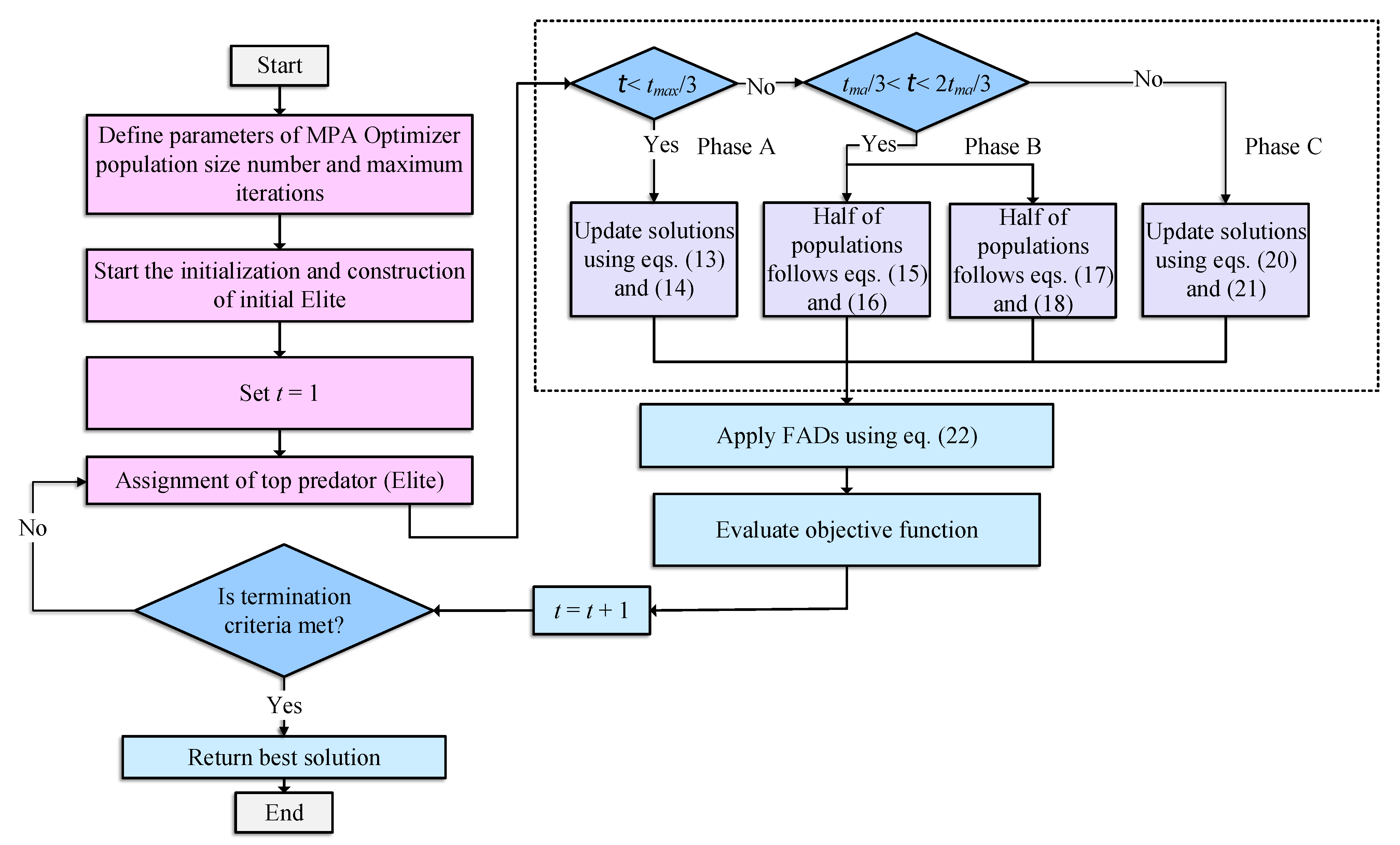
3.3. The MPA Optimization

The MPA has found wide employment in several applications for solving optimization problems [28,45]. The main principle inspiration of MPA is the widespread food-searching strategy through the Levy and Brownie movements in their surrounding predators with optimal encountering of the modified policy based on biological interactions between both the prey and predators. Detailed mathematical modelling of the processes of MPA has been presented in [46]. It benefits the existing good memory by reminding their associates and locations of their successful foraging. It possesses three main phases according to the speed ratio between prey and predators. The flowchart representation of various phases in the MPA optimizer is shown in Figure 5. The phases are explained below.

Phase A (high ratio phase): This phase corresponds to the case when the speed of the prey is higher than the predators. It is employed in the first one-third of the iterations. This phase can be mathematically expressed as follows [46]:

$$S_i=R_{\mathrm{B}}\times (Elit{e}_i-R_{\mathrm{B}}\times Z_i),i=1,2,\dots ,n$$

(13)

$$Z_i=Z_i+P.R\times S_i$$

(14)

where $R\in [0,1]$, and it represents random numbers vector. P = 0.5, and $R_{\mathrm{B}}$ represents the vector of Brownian motion.

Phase B (unity ratio phase): This phase corresponds to the case when the speed of the prey is the same as the speed of the predators. It is employed in the second one-third of the iterations. The movement of predators is expressed by the Brownian expression, whereas the movement of prey is expressed by the Lévy flight modelling approach. In this phase, a division of the population is made into two different subsections. The first one uses (15) and (16), whereas the second section employs (17) and (18) for the modification of their locations, as follows [45]:

$$S_i=R_{\mathrm{L}}\times (Elit{e}_i-R_{\mathrm{L}}\times Z_i),i=1,2,...,n/2$$

(15)

$$Z_i=Z_i+P.R\times S_i$$

(16)

where $R_{\mathrm{L}}$ represents a random variable that is generated by the Lévy distributions.

$$S_i=R_{\mathrm{B}}\times (R_{\mathrm{B}}\times Elit{e}_i-Z_i),i=1,2,...,n/2$$

(17)

$$Z_i=Elit{e}_i+P.CF\times S_i$$

(18)

where

$$CF={(1-\frac{t}{t_{\max }})}^{2\frac{t}{t_{\max }}}$$

(19)

where t and $t_{\max }$ denote the current value and maximum value of the numbers of iterations.

Phase C (low ratio phase): This phase is the opposite of the first phase. This phase corresponds to the case when the speed of the prey is lower than the speed of the predators. It is employed in the last one-third of iterations. In this phase, modifications in the location are made as follows [46]:

$$S_i=R_{\mathrm{L}}\times (R_{\mathrm{L}}\times Elit{e}_i-Z_i),i=1,2,...,n$$

(20)

$$Z_i=Elit{e}_i+P.CF\times S_i,CF={(1-\frac{t}{t_{\max }})}^{2\frac{t}{t_{\max }}}$$

(21)

In [46], the eddy formation and the fish aggregation device effects (FADs) $Fs$ are used to consider the surrounding environment conditions of prey and predators. Thence, the population’s position is modified according to FADs to avoid local optimum solutions. This is expressed as follows:

$$Z_i=\left\{\begin{array}{cc}{Z}_i+CF.[Z_{\min }+R\times (Z_{\max }-Z_{\min })\times W,\hfill & r\le Fs\hfill \\ Z_i+[Fs(1-r)+r](Z_{r1}-Z_{r2}),\hfill & r>Fs\hfill \end{array}\right.$$

(22)

where $Fs$ equals to 0.2, W represents a binary number between 0 and 1, and r denotes a random number, while $r1$ and $r2$ represent random indices for preys. $Z_{\max }$ and $Z_{\min }$ denote the lower- and upper-bound vectors.

3.4. The Proposed Optimization Process

The aforementioned MPA optimizer is utilized for determining the optimized parameter values of the new proposed cascaded TID-FOPIDN LFC control as well as for the TID control of EVs. The optimization process is driven through minimizing the selected fitness function of the optimization process. The three main measures for the optimization process are the frequency deviation in area a ($\Delta F_1$), the deviation in frequency in area b ($\Delta F_1$), and the deviation in the tie-line power between the two areas $\Delta P_{tie12}$. The objective function in the proposed optimization process includes the three measures without weighing factors due to the use of p.u. measures. There are four main representations of objective functions that will be utilized in the proposed optimization process:

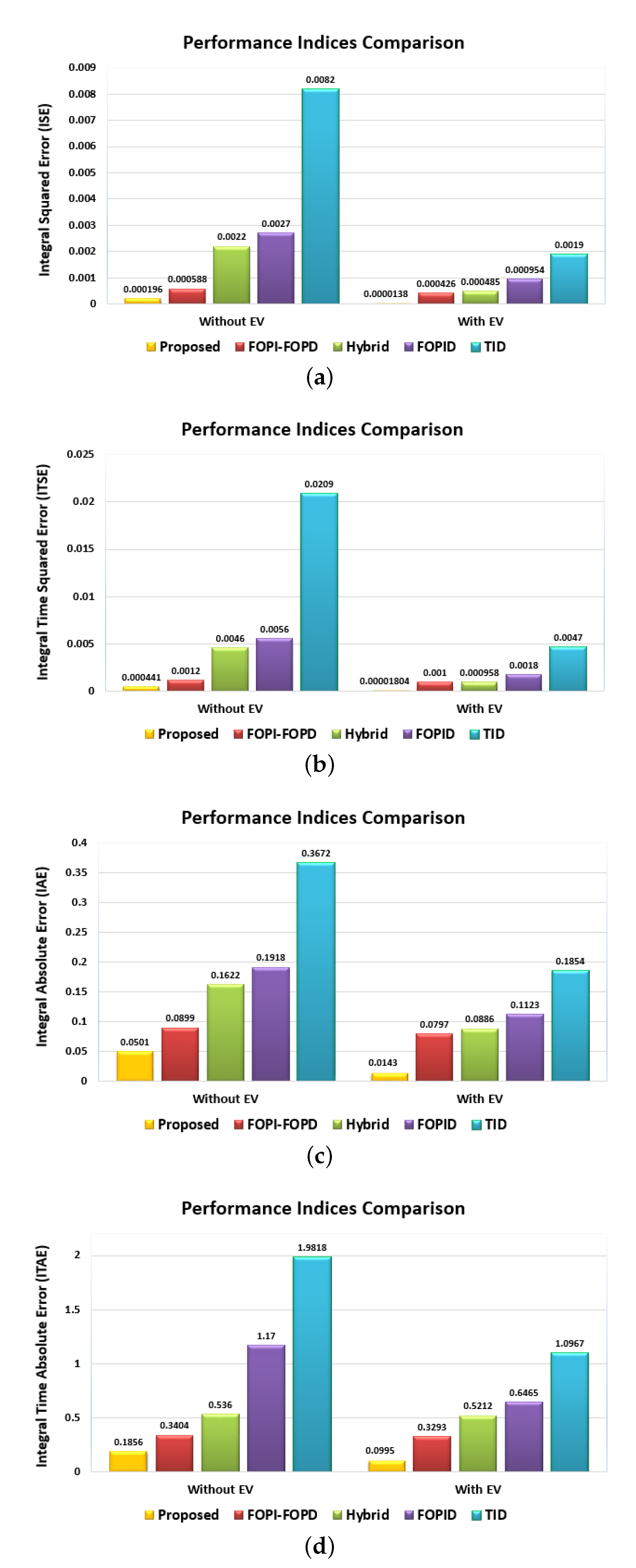
• The integral squared errors (ISE),

  $$\mathrm{I}\mathrm{S}\mathrm{E}=\int \sum _{i=1}^m\left(e_i^2\right)\mathrm{d}t;$$

  (23)
• The integral time squared errors (ITSE),

  $$\mathrm{I}\mathrm{T}\mathrm{S}\mathrm{E}=\int \sum _{i=1}^m\left(e_i^2\right)t.\mathrm{d}t;$$

  (24)
• The integral absolute errors (IAE), and

  $$\mathrm{I}\mathrm{A}\mathrm{E}=\int \sum _{i=1}^{m}abs\left(e_i\right)\mathrm{d}t;$$

  (25)
• The integral time absolute errors (ITAE),

  $$\mathrm{I}\mathrm{T}\mathrm{A}\mathrm{E}=\int \sum _{i=1}^{m}abs\left(e_i\right)t.\mathrm{d}t.$$

  (26)

The above-mentioned objective functions with the targeted minimization of frequency and tie-line power deviations are estimated in the proposed optimization process. Moreover, the measures are used during the time of simulation $t_s$ while considering the various existing limitations. The four objective functions with the targeted control objectives in the two areas can be expressed as follows:

$$\mathrm{I}\mathrm{S}\mathrm{E}=\underset{0}{\overset{t_s}{\int }}({(\Delta f_1)}^2+{(\Delta f_2)}^2+{(\Delta P_{tie})}^2)\mathrm{d}t$$

(27)

$$\mathrm{I}\mathrm{T}\mathrm{S}\mathrm{E}=\underset{0}{\overset{t_s}{\int }}({(\Delta f_1)}^2+{(\Delta f_2)}^2+{(\Delta P_{tie})}^2)t.\mathrm{d}t$$

(28)

$$\mathrm{I}\mathrm{A}\mathrm{E}=\underset{0}{\overset{t_s}{\int }}(abs(\Delta f_1)+abs(\Delta f_2)+abs(\Delta P_{tie}))\mathrm{d}t$$

(29)

$$\mathrm{I}\mathrm{T}\mathrm{A}\mathrm{E}=\underset{0}{\overset{t_s}{\int }}(abs(\Delta f_1)+abs(\Delta f_2)+abs(\Delta P_{tie}))t.\mathrm{d}t$$

(30)

The main process of MPA-based tuning for the parameters of the proposed controller is shown in Figure 6 with the various parameters in area 1 and area 2. The considered limits of the control parameters can be expressed as follows:

$$\begin{array}{c}{K}_p^{min}\le K_{p1},K_{p2}\le K_p^{max}\\ K_t^{min}\le K_{t1},K_{t2},K_{t3},K_{t4}\le K_t^{max}\\ K_i^{min}\le K_{i1},K_{i2},K_{i3},K_{i4},K_{i5},K_{i6}\le K_i^{max}\\ K_d^{min}\le K_{d1},K_{d2},K_{d3},K_{d4},K_{d5},K_{d6}\le K_d^{max}\\ n^{min}\le n_1,n_2,n_3,n_4\le n^{max}\\ {\lambda }^{min}\le {\lambda }_1,{\lambda }_2\le {\lambda }^{max}\\ {\mu }^{min}\le {\mu }_1,{\mu }_2\le {\mu }^{max}\\ N_c^{min}\le N_{c1},N_{c2}\le N_c^{max}\end{array}$$

(31)

where the minimum values of control parameters are represented by $min$, and the maximum limits are expressed by $max$ in the constraints of the proposed cascaded TID-FOPIDN controller. The minimum values of control gains ($K_t^{min}$, $K_i^{min}$, and $K_d^{min}$) are selected to be equal to zero, and the their maximum values ($K_t^{max}$, $K_i^{max}$, and $K_d^{max}$) are selected to be equal to 5 in the proposed optimization process. The minimum and maximum values ($n^{min}$ and $n^{max}$) are adjusted to be 2 and 5, respectively. The minimum values of (${\lambda }^{min}$, and ${\mu }^{min}$) are set to be zero, while their maximum values (${\lambda }^{max}$, and ${\mu }^{max}$) are set to be 1. The minimum and maximum values ($N_c^{min}$ and $N_c^{max}$) are selected to be equal to 5 and 500, respectively.

4. Simulation Results and Performance Verification

The studied model of the interconnected multi-source, multi-area power system, illustrated in Figure 1, was developed using the MATLAB software with the Simulink tool and implementing the m.file code, which contains the MPA technique with different objective function computations. The optimization algorithms were tested by using a number of populations equal to 20 with a maximum iteration number of 100 times. The MATLAB code file was interfaced with the simulation file of the multi-area power system model to execute the process of tuning all the control parameters of the suggested controllers. In this paper, the initialization functions presented by the main authors of the optimization algorithms were employed. The TID, FOPID, hybrid, FOPI-FOPD, and the proposed TID-FOPIDN methods in each area were selected for performance comparison. In addition, the controller gains of the EVs under different disturbance scenarios of load and RES variations were also optimized simultaneously using the optimizer algorithms.

To evaluate the performance of the proposed control approach based on the MPA, it was compared with conventional TID, FOPID, the advanced hybrid fractional controller, and the cascaded FOPI-FOPD controller. Furthermore, the MPA technique’s convergence performance was examined and compared with other metaheuristic algorithms, such as manta ray foraging optimization (MRFO), particle swarm optimization (PSO), genetic algorithm (GA), and artificial ecosystem optimization (AEO). The results and analysis were performed on a personal computer with an Intel Core i7 CPU of 2.9 GHz, 64-bit version. Figure 7 shows the comparison in the case of step load perturbation without EVs, whereas Figure 8 shows the results with the scenario of step load perturbation with EVs. It is clear that the fast convergence of the MPA algorithm occurred with the minimized fitness function in both cases. For the case with EV, the MPA has the lowest value of the ISE fitness function. The obtained optimum parameters of various elements of the new proposed TID-FOPIDN controller and the existing controllers are summarized in

Table 3. The optimized control parameters of the various studied controllers without EV incorporation using the MPA algorithm.

Controller	Area	Control	Coefficients
			${\mathit{K}}_{\mathit{t}}$	${\mathit{K}}_{\mathit{i}1}$	${\mathit{K}}_{\mathit{d}1}$	${\mathit{K}}_{\mathit{p}1}/{\mathit{K}}_{\mathit{p}2}$	${\mathit{K}}_{\mathit{i}2}$	${\mathit{K}}_{\mathit{d}2}$	n	$\mathit{Nc}$	$\mathit{\lambda }$	$\mathit{\mu }$
Proposed	Area 1	LFC	1.9674	0.6976	1.57	0.33289	0.92242	0.80982	3.8677	245.0444	0.45757	0.5531
	Area 2	LFC	1.9358	0.3844	0.7888	1.3744	0.71797	1.3931	4.6014	300	0.46516	0.55918
Hybrid [24]	Area 1	LFC	2.0000	1.9943	1.3884	-	-	-	3	-	0.955	1.3646
	Area 2	LFC	0.0012	0.3572	1.9997	-	-	-	2.9537	-	0.0008	1.2693
TID [38]	Area 1	LFC	0.1884	0.1238	0.4095	-	-	-	3	-	-	-
	Area 2	LFC	0.2239	0.1131	0.4990	-	-	-	3	-	-	-
FOPID [38]	Area 1	LFC	-	-	-	0.8615	1.8463	1.9990	-	-	0.6494	0.9990
	Area 2	LFC	-	-	-	0.0510	0.3561	1.6478	-	-	0.4003	0.9826
FOPI-FOPD [47]	Area 1	LFC	-	-	-	2/1.8732	2	1.5629	-	-	0.8606	0.0997
	Area 2	LFC	-	-	-	2/1.9725	2	1.998	-	-	0.5130	0.0310

for the case without EVs and in

Table 4. The optimized control parameters of the various studied controllers with EV incorporation using the MPA algorithm.

Controller	Area	Control	Coefficients
			${\mathit{K}}_{\mathit{t}}$	${\mathit{K}}_{\mathit{i}1}$	${\mathit{K}}_{\mathit{d}1}$	${\mathit{K}}_{\mathit{p}1}/{\mathit{K}}_{\mathit{p}2}$	${\mathit{K}}_{\mathit{i}2}$	${\mathit{K}}_{\mathit{d}2}$	n	$\mathit{Nc}$	$\mathit{\lambda }$	$\mathit{\mu }$
Proposed	Area 1	LFC	1.037	1.7698	1.5695	1.3481	1.0339	0.57491	4.0673	296.7003	0.60512	0.93462
		EV	1.745	1.5096	0.40002	-	-	-	2.3908	-	-	-
	Area 2	LFC	1.5215	0.246	0.69809	0.75802	0.98775	0.10823	4.3335	295.7854	0.62899	0.73299
		EV	1.193	1.2462	0.60999	-	-	-	3.116	-	-	-
Hybrid	Area 1	LFC	1.2906	1.063	1.6957	-	-	-	3.6475	-	0.77626	0.90608
		EV	1.9722	1.9295	1.2382	-	-	-	4.4185	-	-	-
	Area 2	LFC	1.0859	0.68601	1.2588	-	-	-	4.8724	-	0.60716	0.10543
		EV	1.7877	0.5144	0.12329	-	-	-	3.5308	-	-	-
TID	Area 1	LFC	1.6069	0.97697	1.6355	-	-	-	2.9463	-	-	-
		EV	1.9995	1.9586	0.44039	-	-	-	4.0746	-	-	-
	Area 2	LFC	0.55574	1.5664	1.7384	-	-	-	3.2124	-	-	-
		EV	1.481	0.67578	1.5763	-	-	-	2.6727	-	-	-
FOPID	Area 1	LFC	-	-	-	1.057	1.7666	1.5353	-	-	0.74518	0.94931
		EV	1.9581	1.8882	1.5734	-	-	-	3.486	-	-	-
	Area 2	LFC	-	-	-	0.44181	1.0682	0.32657	-	-	0.42262	0.45609
		EV	1.8372	0.97982	1.529	-	-	-	3.5885	-	-	-
FOPI-FOPD	Area 1	LFC	-	-	-	2/1.9991	2	1.6731	-	-	0.7421	0.2451
		EV	0.17532	0.1421	0.5197	-	-	-	2.753	-	-	-
	Area 2	LFC	-	-	-	2/1.342	2	1.989	-	-	0.7845	0.04710
		EV	0.3517	0.1982	0.6781	-	-	-	3.691	-	-	-

for the case with EVs.

These results are organized to cover the following scenarios:

• Scenario 1: The impact of step load perturbation (SLP) with and without EVs;
• Scenario 2: The impact of SLP under the generation outage effects;
• Scenario 3: The impact of uncertainties in the power system inertia;
• Scenario 4: The impact of random load pattern;
• Scenario 5: The impact of RES fluctuations and load variations.

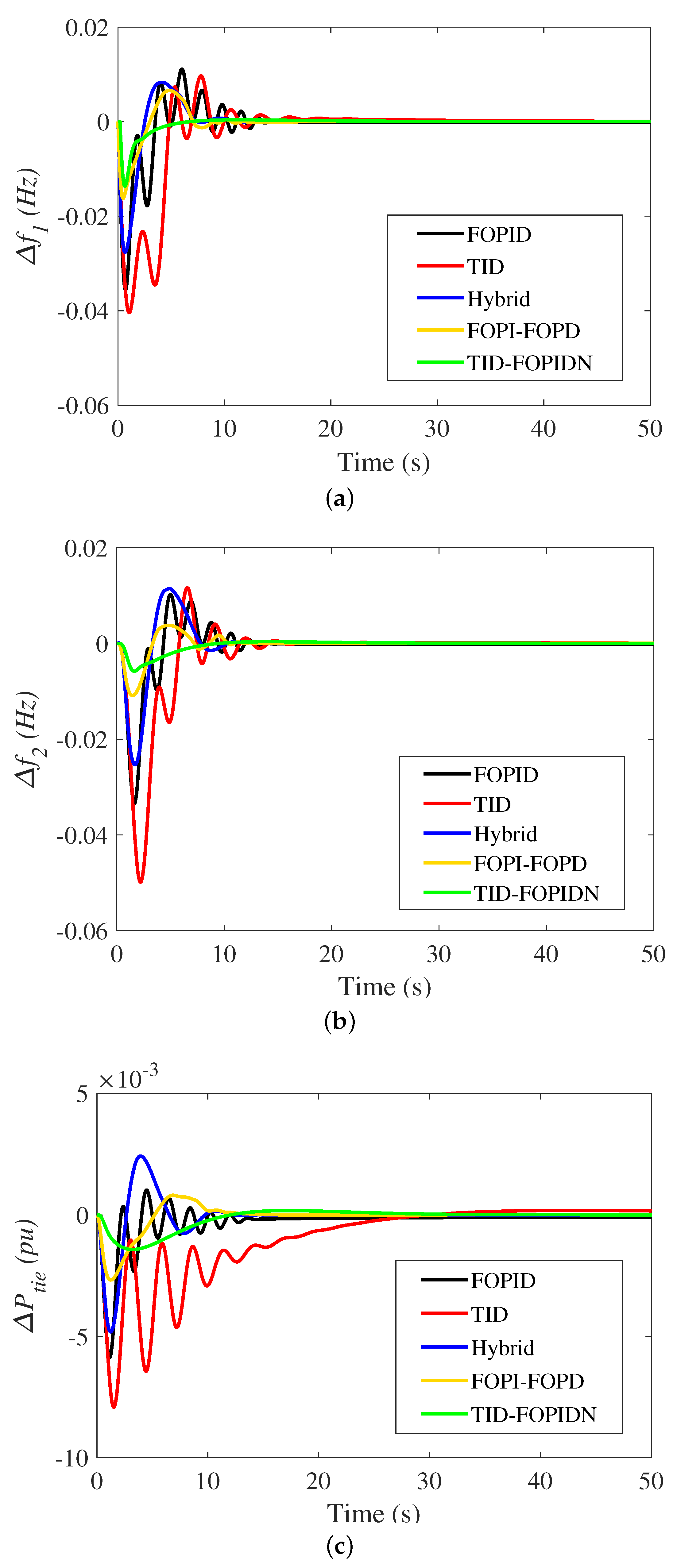
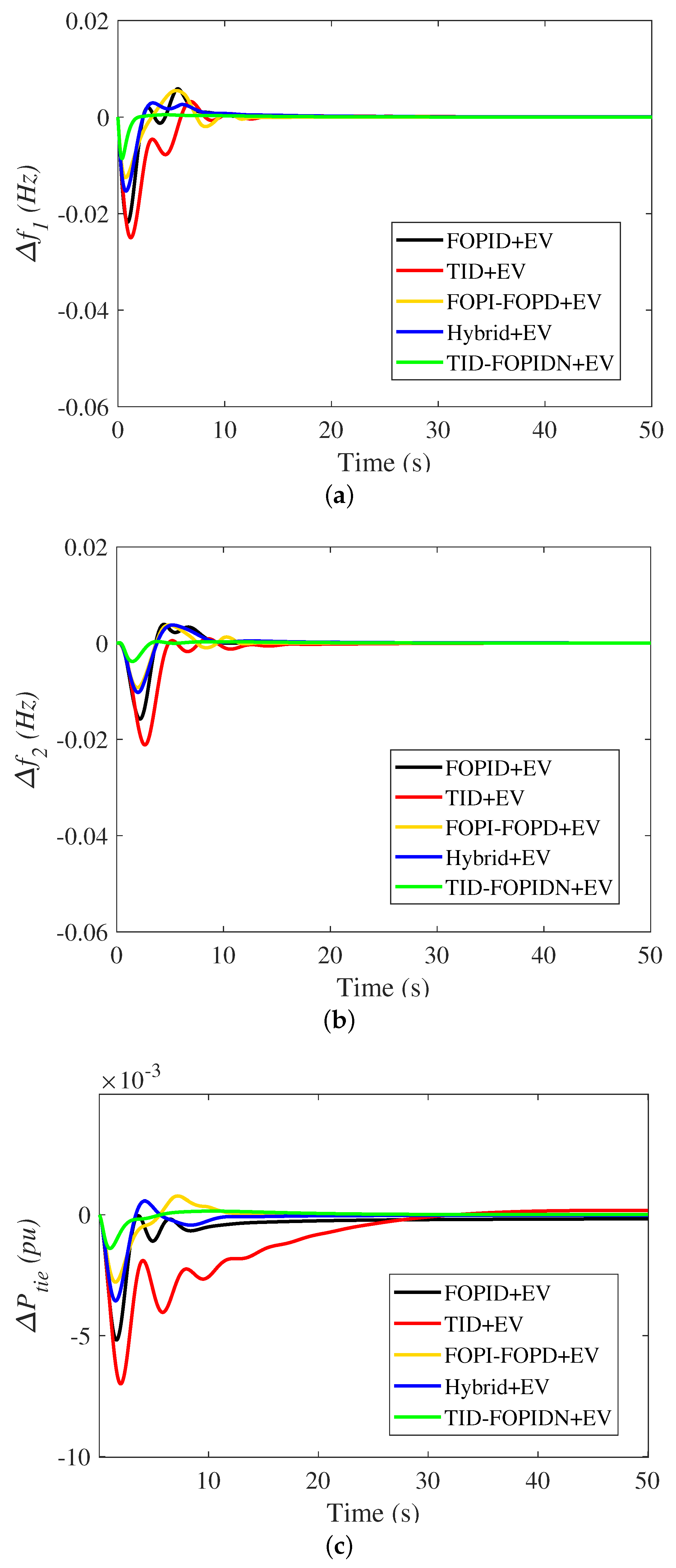
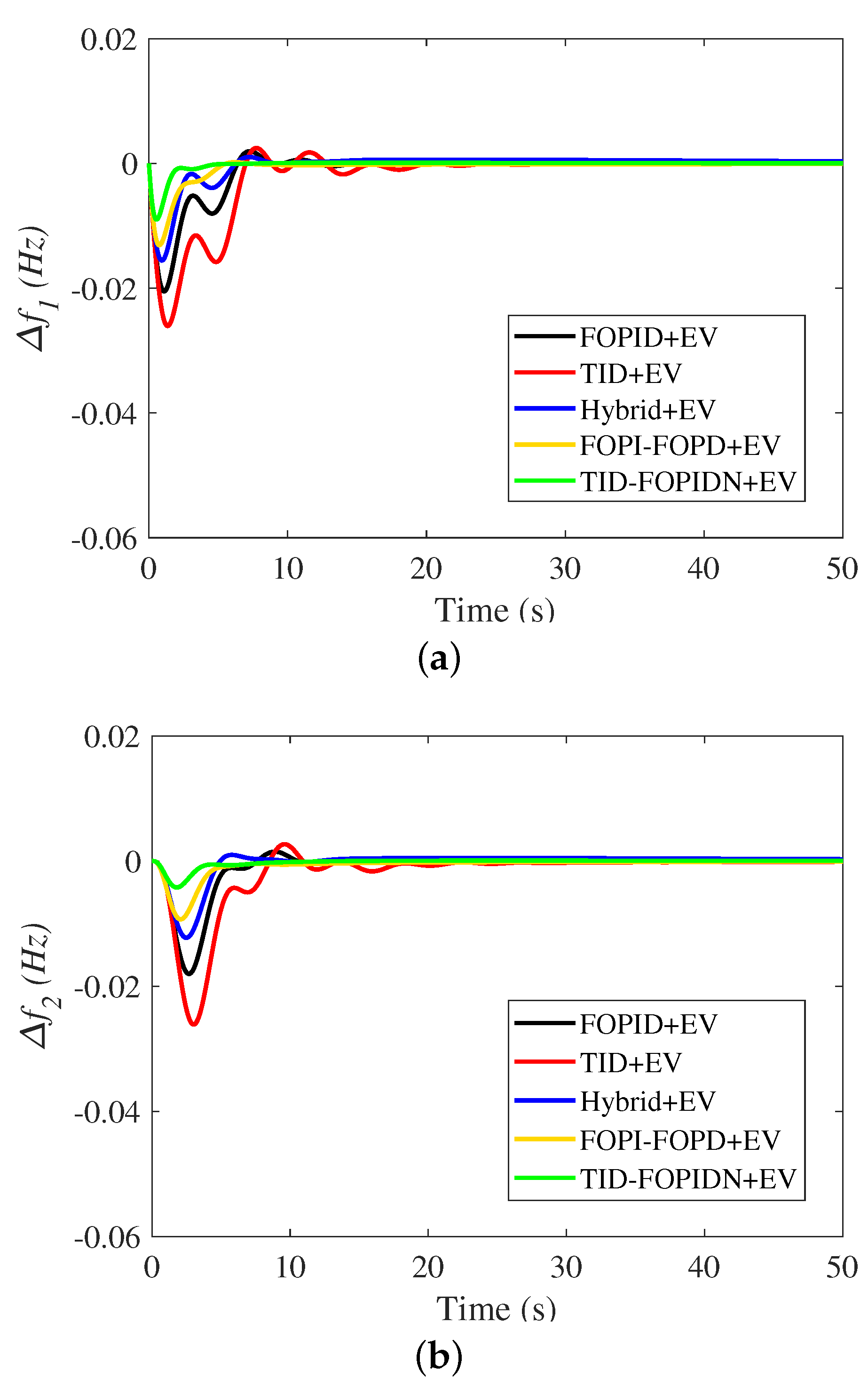
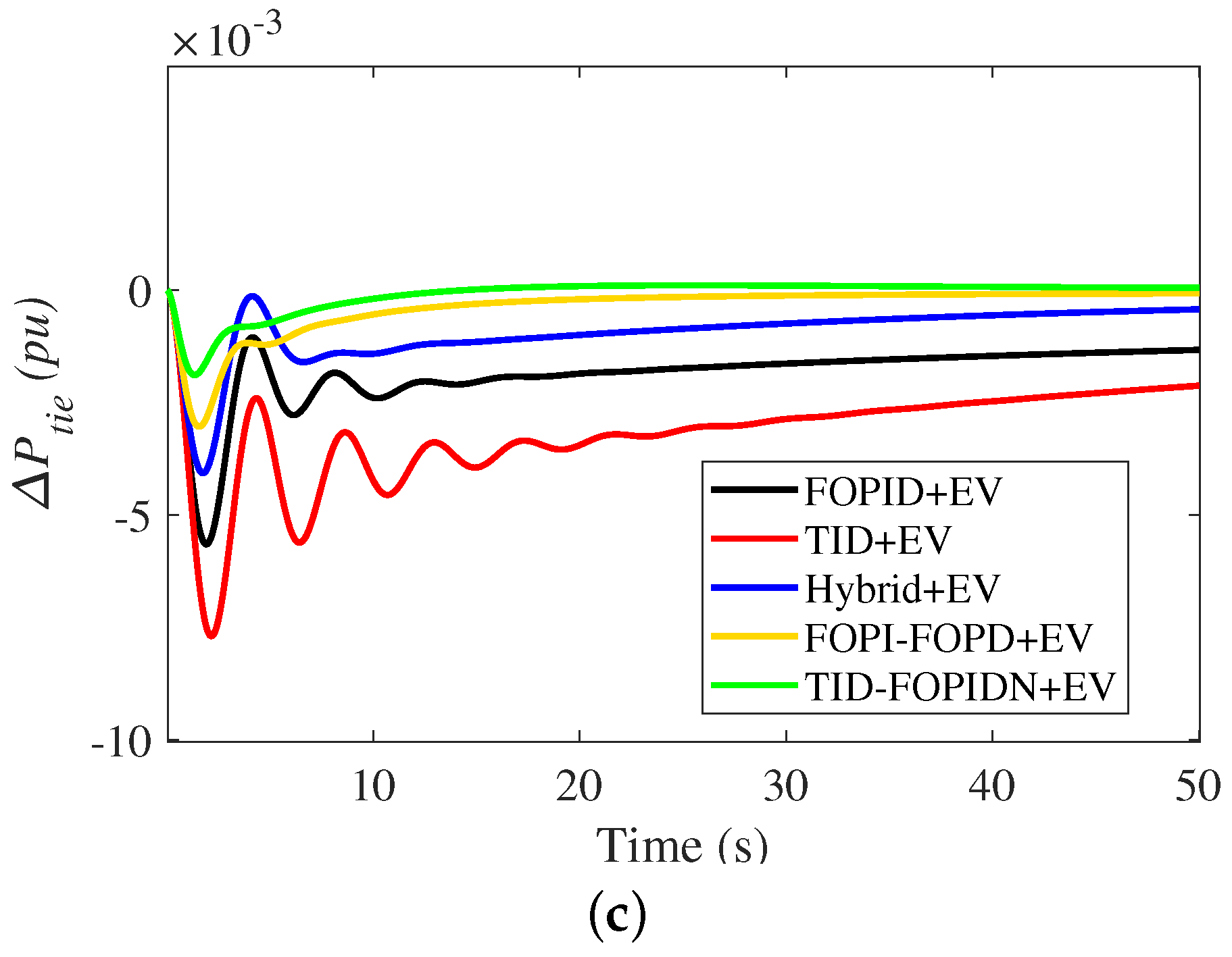
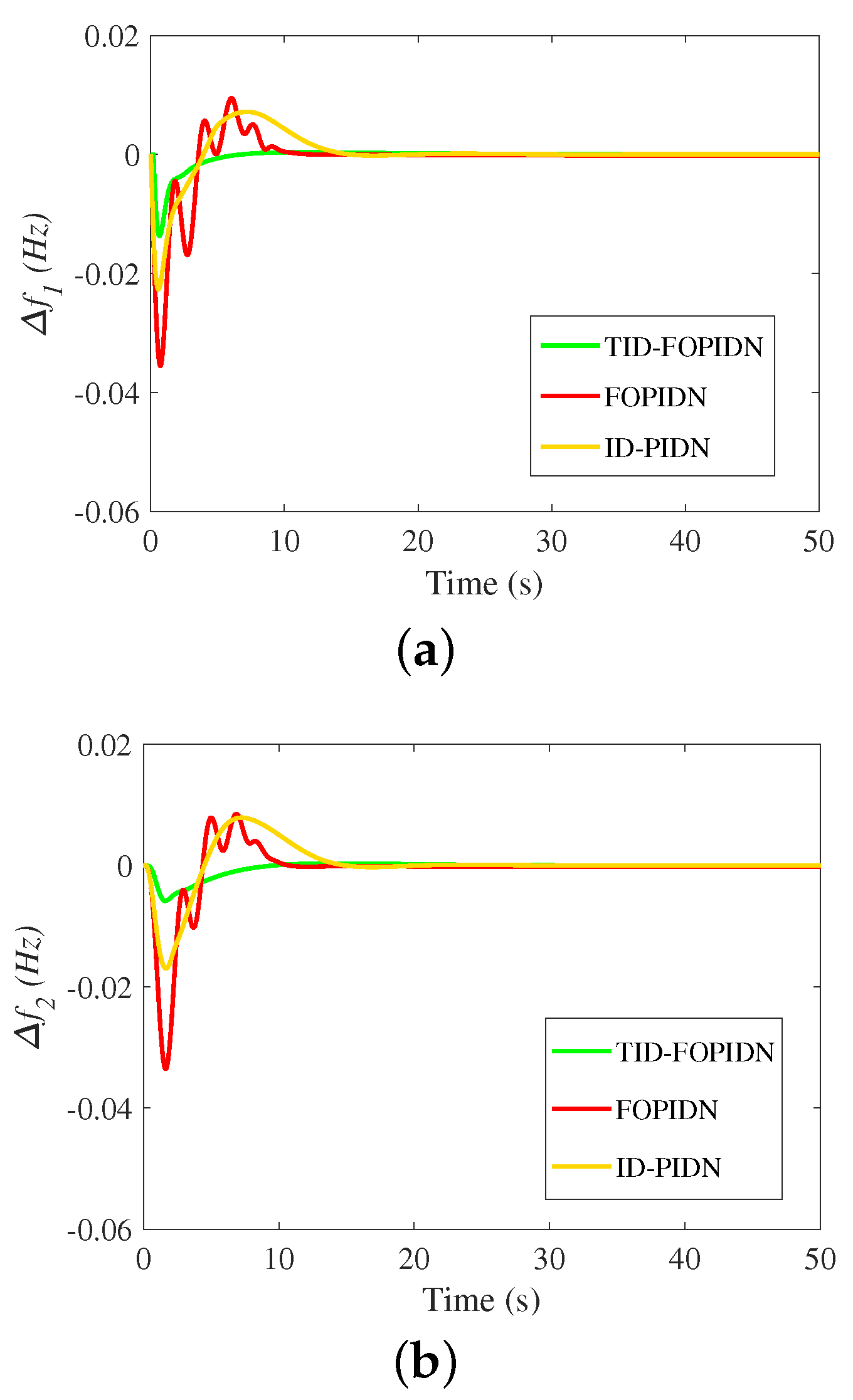
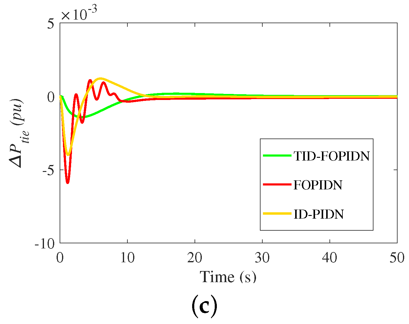
4.1. Scenario 1: Impact of SLP

This subsection presents the first test scenario for the studied multi-source multi-area power system to validate the effectiveness of the proposed TID-FOPIDN controller based on the MPA algorithm over the other existing conventional and advanced techniques that are introduced in the literature as a means of comparison. In this case, the studied power system was investigated at 1% SLP at area 1 at t = zero seconds while disconnecting the RESs and EVs from the system to assure a fair comparison with other previously presented control techniques in the literature. Figure 9 visualizes the studied power system responses, such as frequency deviations in both area 1 and area 2 ($\Delta f_1$, $\Delta f_2$, and the tie-line power waveform between the two areas $\Delta P_{tie}$), respectively. In addition,

Table 5. Settling times (ST), peak undershoots (PU), and peak overshoots (PO) for tested scenarios.

Scenario	Controller	$\Delta {\mathit{f}}_1$			$\Delta {\mathit{f}}_2$			$\Delta {\mathit{P}}_{\mathbf{tie}}$
		PO	PU	ST (s)	PO	PU	ST (s)	PO	PU	ST (s)
No.1 1% SLP without EV	TID	0.0096	0.0404	29	0.0116	0.0498	25	0.0002	0.0079	33
	FOPID	0.0111	0.0355	21	0.0103	0.0334	20	0.0011	0.0059	15
	Hybrid	0.0085	0.0277	15	0.0114	0.0253	14	0.0024	0.0048	14
	FOPI-FOPD	0.0066	0.0162	13	0.0038	0.0109	11	0.0008	0.0026	18
	Proposed	0.0004	0.0136	8	0.0002	0.0057	9	0.0001	0.0014	12
No.1 1% SLP with EV	TID	0.0032	0.0249	16	0.0009	0.0211	22	0.0002	0.0069	30
	FOPID	0.0058	0.0217	15	0.0039	0.0157	10	0.0001	0.0052	35
	Hybrid	0.0029	0.0153	13	0.0037	0.0103	9	0.0002	0.0431	17
	FOPI-FOPD	0.0052	0.0125	14	0.0036	0.0092	13	0.0005	0.0036	19
	Proposed	―	0.0084	5	0.0003	0.0037	6	0.0001	0.0013	11
No.2 1% SLP Outage	TID	0.0025	0.0261	27	0.0027	0.0261	26	―	0.0077	>50
	FOPID	0.0019	0.0205	19	0.0015	0.0181	18	0.0024	0.0056	>50
	Hybrid	0.001	0.0156	16	0.0009	0.0123	14	0.0014	0.0041	>50
	FOPI-FOPD	0.0002	0.0131	12	―	0.0093	12	0.001	0.0031	>50
	Proposed	0.0001	0.0088	9	0.0002	0.0042	10	―	0.0018	12
No.4 at 30 s	TID	0.0591	0.2651	55	0.0464	0.2554	52	0.0103	0.0754	76
	FOPID	0.0385	0.2031	51	0.0286	0.1666	49	0.0013	0.0516	48
	Hybrid	0.0155	0.1421	47	0.0238	0.1078	43	0.0011	0.0351	41
	FOPI-FOPD	0.0281	0.1271	23	0.0214	0.0945	21	0.0034	0.0304	28
	Proposed	0.0002	0.0851	13	0.0034	0.0444	13	0.0016	0.0171	17
No.5 at 10 s	TID	0.2542	0.0501	57	0.2345	0.0473	56	0.0089	0.0632	67
	FOPID	0.2014	―	>120	0.1977	―	>120	―	0.0502	>120
	Hybrid	0.1264	―	>120	0.1728	―	>120	―	0.0541	>120
	FOPI-FOPD	0.0955	0.0211	28	0.1205	0.0295	24	0.0036	0.0285	25
	Proposed	0.0331	―	23	0.1021	0.0212	21	0.0021	0.0251	25

shows the values of different criteria, such as the settling time (Ts), maximum overshoot (MO), and maximum undershoot (MU). From these data, the superiority of the proposed MPA with the TID-FOPIDN controller is evident.

In this case study, the value of the frequency deviations in the studied system with the TID controller was retained to 0.041 Hz for area 1 and 0.049 Hz for area 2 with tie-line power deviation within 0.0079 p.u. The FOPID maintained the system frequency at 0.0356 Hz for area 1 and 0.0334 Hz for area 2 with a tie-line power deviation of 0.0058 p.u during the load disturbance of 1% change. However, the hybrid FO controller gave a better performance than the TID and FOPID by decreasing the system frequency aberration of the studied multi-area system to 0.0276 Hz for area 1 and 0.0253 Hz for area 2 while keeping the power variation value at 0.0048 p.u. Otherwise, the cascaded structure controllers have a superior performance, as the FOPI-FOPD controller has lower frequency and tie-line power oscillations than the other controllers. From another perspective, the proposed TID-FOPIDN has the best performance regarding lowering the overshoot and undershoot values. The new proposed MPA-based TID-FOPIDN achieves the fastest controller in repression of the power and frequency fluctuations compared to TID, FOPID, hybrid, and FOPI-FOPD controllers, as summarized in Table 5.

On the other hand, Figure 10 shows the impact of the deployment of EVs on the dynamic performance of the multi-source multi-area power system. It can be noted that the system frequency and tie-line power deviations have a better damping response than the previous case without EVs. This, in turn, identifies the EVs’ participation in the LFC loop due to their energy-storing property and their participation. It is observed from this figure that the new proposed TID-FOPIDN controller coordinated with the charging/discharging of EVs in both areas has effectively succeeded in damping the oscillations of the system frequency and power. The new proposed MPA-based TID-FOPIDN controller has the lowest overshoot and undershoot values and the fastest settling time compared with the other featured controllers in the literature. Furthermore, the robustness of the proposed controller is proved in Figure 11 in terms of the ISE, ITSE, IAE, and ITAE objective functions of this scenario.

On the other hand,

Table 6. Comparison of performance indices for the various controllers.

Scenario	Controller Technique	Performance Indices
		ISE	ITSE	IAE	ITAE
No. 1 (1% SLP without EV)	TID	0.0082	0.0209	0.3672	1.9818
	FOPID	0.0027	0.0056	0.1918	1.17
	Hybrid	0.0022	0.0046	0.1622	0.536
	FOPI-FOPD	0.000588	0.0012	0.0899	0.3404
	Proposed	0.000212	0.000441	0.0501	0.1856
No. 1 (1% SLP with EV)	TID	0.0019	0.0047	0.1854	1.0967
	FOPID	0.000954	0.0018	0.1123	0.6465
	Hybrid	0.000485	0.000958	0.0886	0.5212
	FOPI-FOPD	0.000426	0.001	0.0797	0.3293
	Proposed	0.0000138	0.00001804	0.0143	0.0995

proves the ability of the proposed MPA-based cascaded TID-FOPIDN controller for the LFC and EV processes. The new proposed TID-FOPIDN controller achieves the best values for the performance metrics of the estimated indices, such as ISE, ITSE, IAE and ITAE, in comparison with the other classical and advanced controllers in the literature.

4.2. Scenario 2: The Impact of Generation Outage

The main goal of this scenario was to test the performance of the suggested two area multi-source power system and the performance of the proposed frequency controller. In this scenario, an extreme disturbance of generation unit outage was applied to the studied system. Therefore, this case considered a cascaded failure by disconnecting the thermal and hydraulic generation units. Figure 12 shows high deviations of system frequency and tie-line power in this case due to the imbalance between generation and demand. It can be observed that, in the case of using the TID controller, the system exhibits poor damping characteristics for the deviations in the system frequency and tie-line power during this terrible fault. Furthermore, the FOPID and hybrid controllers show slightly lower peak values of frequency deviations compared to the TID controller, but they still suffer from long settling time values for tie-line power oscillations, as detailed in Table 5. On the other hand, the cascaded structures of FOPI-FOPD and TID-FOPIDN controllers have an improved dynamic response in restoring the frequency and tie-line power deviations compared to the other studied control techniques. However, the proposed controller has the fastest action with minimum system deviations. This scenario also indicates the effective role of the EVs in reserve power compensation as they can quickly discharge the required power at the instant of generation outage, and thence, damping of the tie-line power variations is obtained. Therefore, it can be noted from these results that the proposed MPA-based TID-FOPIDN controller provides more stable and faster performance in restoring the frequency and tie-line power deviations compared with the other studied control techniques.

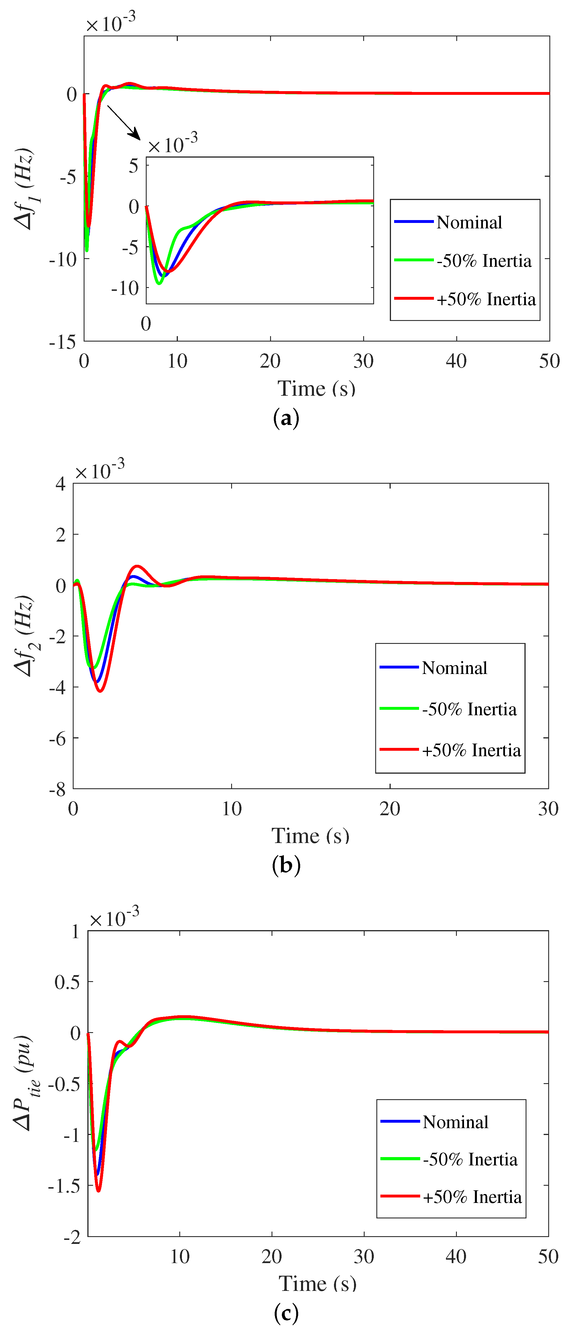
4.3. Scenario 3: The Impact of Uncertainties in the Power System Inertia

This scenario tested the impact of inertia reduction on the interconnected multi-source power system. This scenario was selected because reducing the system inertia can generate high frequency and voltage fluctuations. In this scenario, a 1% SLP was applied considering an uncertainty situation of a 50% decrease in power system inertia. The effect of the multi-area frequency performance against the reduction in system inertia was tested. Figure 13 shows more frequency fluctuations and larger transient deviations of the studied system during the low system inertia condition. It can be seen from this figure that the proposed coordination of LFC using the proposed MPA-based TID-FOPIDN and EV participation can enhance the dynamic frequency performance. Moreover, it can diminish the transient excursion with a fast response regarding the disturbance refutation, tracking attribute, and minimum steady-state error during the uncertainty condition of ± 50% of system inertia. Therefore, it can be concluded that for the low system inertia condition, the designed LFC of TID-FOPIDN and power sharing from the EVs is more efficient at managing the abrupt load changes and tracks the operating point of the multi-area power system. Consequently, these results indicate the significant role of EVs in supporting the system frequency during highly disrupting conditions.

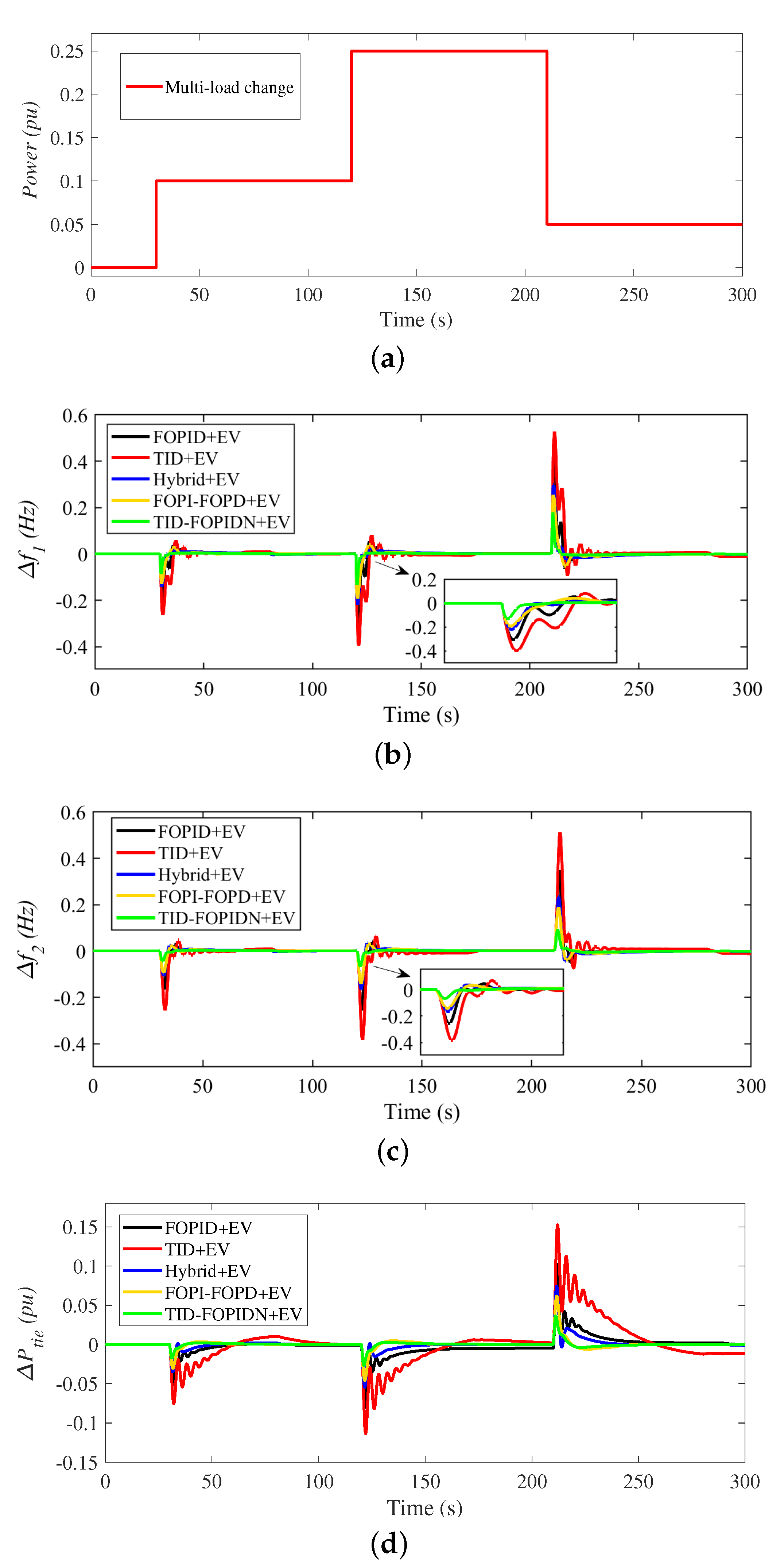
4.4. Scenario 4: The Impact of Multi-Step Load

In this case, the capability of the proposed coordination of LFC and EVs using the TID-FOPIDN controller based on the MPA technique was evaluated and revealed under the impact of a drastic multi-step load change pattern, as shown in Figure 14d. The interconnected multi-area multi-source system incurred multi-load disturbances of a 10% decrease, 15% decrease, and 20% increase at time t = 30 s, 120 s, and 210 s, respectively. To verify the durability of the proposed optimized TID-FOPIDN controller, it was compared with the conventional TID and FOPID controllers in addition to the advanced hybrid controller and cascaded FOPI-FOPD controller. Figure 14 shows the system frequency and power waveforms of the proposed multi-area power system during the impact of multi-step load variations. It is clear that the dynamic responses of the proposed LFC strategy coordinated with the EV cooperation have faster control actions with minimized deviations compared to other proposed control techniques.

The new proposed controller can properly keep the frequency deviations within −0.085 Hz for area 1 and −0.044 Hz for area 2 at time t = 30 s with fast and smooth settling time. Conversely, the cascaded FOPI-FOPD controller came in second place with frequency deviations of about −0.123 Hz in area 1 and −0.095 Hz for area 2 with a deviation of −0.031 p.u in tie-line power, as summarized in Table 5. The hybrid fractional order controller came in third place after the two cascaded controllers through maintaining the frequency at −0.142 Hz in area 1 and −0.107 Hz in area 2. However, utilizing the TID and FOPID controllers can restore the system frequency and tie-line power deviations, although with long settling time and high oscillations of overshoot and undershoot of more than ±0.3 Hz, especially at 120 s and 210 s with high load variation at ±15%. Therefore, it is obvious from the above-mentioned discussion that improved results with the best performance metrics are obtained from the coordination of LFC and EV sharing systems using the new proposed MPA-based optimized cascaded TID-FOPIDN controller.

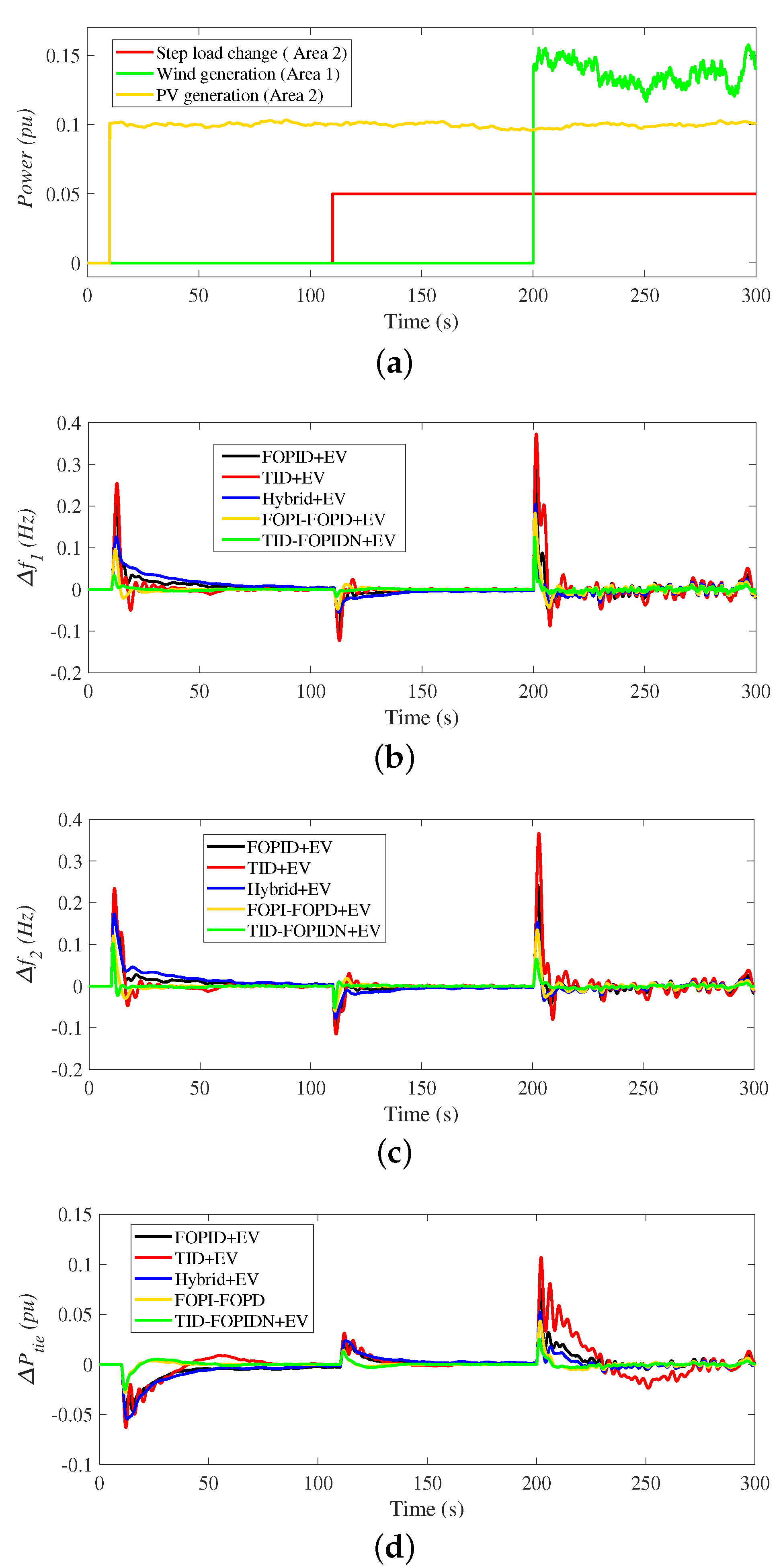
4.5. Scenario 5: The Impact of RES Fluctuations

This scenario considers further validation of the new proposed new cascaded controller performance and its coordination with the EVs sharing level. In this scenario, the renewable energy sources (RESs) with their variability and intermittency in the generation were addressed during the assessment of the transient stability of the multi-area hybrid power system. Both wind and PV power plants were employed in the first and second areas of the system, as presented in the system structure in Figure 1. In addition, a step load of 5% was applied in area 2. The changes in wind, PV, and load power are depicted in Figure 15a. The dynamic performance of ($\Delta f_1$, $\Delta f_2$, and ${\Delta }_{Ptie}$) for all the compared controllers in this scenario is evaluated in Figure 15.

It can be observed that at the integration instant of the PV generation system at the time of 10 s, frequency deviations in both area 1 and area 2 increase temporarily due to the surplus power generation from the PV system. The superior performance of the new proposed TID-FOPIDN controller with the EV participation is clear. It can also be seen that the conventional TID and FOPID controllers have frequency deviation levels of more than 0.2 Hz at 10 s and more than 0.3 Hz at the instant of wind generation insertion at 210 s. In addition, the hybrid FO controller can reduce deviation levels to nearly 0.135 Hz, which is relatively better than TID and FOPID controllers.

From another perspective, the cascaded FOPI-FOPD controller maintains the frequency deviation around 0.1 Hz with faster performance than the above-mentioned controllers. The new proposed cascaded TID-FOPIDN controller can preserve the system stability by reducing the frequency fluctuations to lower than 0.1 Hz at the PV connection time of 10 s, lower than 0.12 Hz at the time of wind generation connection, and around 0.05 p.u. in the tie-line power, as summarized in Table 5. Additionally, an improved system response and enhanced functionality are obtained when the EV elements are considered despite uncertainties in the hybrid generation units.

4.6. Additional Comparisons

Additional comparisons of the proposed cascaded TID-FOPIDN controller are preformed with the integer order version (cascaded ID-PIDN) controller and the FOPIDN controller. The comparisons are made using scenario 1 with a 1% SLP case study. Figure 16 and Figure 17 show the obtained results for the case studies without and with EV, respectively. It is clear that the proposed cascaded TID-FOPIDN controller achieves lower undershoot values compared with the high undershoot values under the FOPIDN controller. The benefits come from using the additional frequency signal, which enables the proposed controller to damp the low-frequency and the high-frequency disturbances. Conversely, using only the ACE signal can only damp the low-frequency disturbances. Moreover, the results show better damping using the proposed controller compared to the integer order cascaded ID-FOPIDN controller. The improvements come from the additional tunable parameters of the FO operators in the proposed controller.

5. Conclusions

A novel implementation of a cascaded TID-FOPIDN controller is presented in this paper to enhance the LFC of a multi-area electrical power network consisting of multiple sources. In addition, the incorporation of mixed renewable generators and electrical vehicles are considered in this paper with the fluctuations in RES generation and uncertainties in power system inertia. The recently introduced MPA method is applied for tuning the parameters of the new proposed cascaded TID-FOPIDN controller, and the TID controller is also tuned simultaneously using the MPA to control EVs in each area. The proposed TID-FOPIDN is validated against the existing nonlinearities, uncertainties, and load/generation variations in the studied multi-area multi-source power system. The conditions of the existence/absence of EVs in the studied system are considered in the validation of system performance. Moreover, comprehensive comparisons of the new proposed TID-FOPIDN controller with the featured LFC methods in the literature are presented in the paper. The obtained results verify that the proposed cascaded TID-FOPIDN controller is proven to be more efficient than the studied conventional TID and FOPID controllers, the advanced hybrid, and cascaded FOPI-FOPD controllers. The obtained comparisons of ISE, ITSE, IAE, and ITAE objective functions based on the simulated results prove the minimized frequency and tie-line power deviations using the proposed optimized TID-FOPIDN controller. At 1% sLP with EV, the proposed cascaded TID-FOPIDN controller achieves a minimum ISE value of 0.0000138 compared to 0.0019, 0.000954, 0.000485, and 0.000426 for the TID, FOPID, hybrid, and FOPI-FOPD controllers, respectively. In addition, the proposed controller achieves an ITAE of 0.0995 compared with 1.0967, 0.6465, 0.5212, and 0.3293 for the TID, FOPID, hybrid, and FOPI-FOPD controllers, respectively. Based on the designed optimized controllers, the coordination of the LFC and installed EVs is achieved to maintain the multi-area power system stability during the various existing disturbance in power systems. Therefore, the proposed MPA-based optimized TID-FOPIDN controller can achieve enhanced performance in regulating the power system frequency and enhancing the dynamical behavior of multi-area, multi-source electrical power systems with high penetration levels of RESs. However, the proposed controller possesses extra added tunable parameters, which can lead to more complex computation burdens in the design and implementation stages for a higher number of interconnected areas. Thanks to the recently developed powerful software and hardware computing devices, the design and implementation processes have become possible and feasible. Future research suggestions include comparing the various obtained results with unifying the initialization function of all the optimization algorithms.

References

1. Said, S.M.; Aly, M.; Hartmann, B.; Alharbi, A.G.; Ahmed, E.M. SMES-Based Fuzzy Logic Approach for Enhancing the Reliability of Microgrids Equipped With PV Generators. IEEE Access 2019, 7, 92059–92069. [Google Scholar] [CrossRef]
2. REN21. Renewables 2021: Global Status Report. 2019. Available online: https://www.ren21.net/reports/global-status-report/ (accessed on 1 June 2022).
3. Siti, M.; Mbungu, N.; Tungadio, D.; Banza, B.; Ngoma, L. Application of load frequency control method to a multi-microgrid with energy storage system. J. Energy Storage 2022, 52, 104629. [Google Scholar] [CrossRef]
4. Irudayaraj, A.X.R.; Wahab, N.I.A.; Premkumar, M.; Radzi, M.A.M.; Sulaiman, N.B.; Veerasamy, V.; Farade, R.A.; Islam, M.Z. Renewable sources-based automatic load frequency control of interconnected systems using chaotic atom search optimization. Appl. Soft Comput. 2022, 119, 108574. [Google Scholar] [CrossRef]
5. Hu, Z.; Liu, S.; Wu, L. Credibility-based distributed frequency estimation for plug-in electric vehicles participating in load frequency control. Int. J. Electr. Power Energy Syst. 2021, 130, 106997. [Google Scholar] [CrossRef]
6. Said, S.M.; Aly, M.; Hartmann, B.; Mohamed, E.A. Coordinated fuzzy logic-based virtual inertia controller and frequency relay scheme for reliable operation of low-inertia power system. IET Renew. Power Gener. 2021, 15, 1286–1300. [Google Scholar] [CrossRef]
7. da Silva, G.S.; de Oliveira, E.J.; de Oliveira, L.W.; de Paula, A.N.; Ferreira, J.S.; Honório, L.M. Load frequency control and tie-line damping via virtual synchronous generator. Int. J. Electr. Power Energy Syst. 2021, 132, 107108. [Google Scholar] [CrossRef]
8. Ranjan, M.; Shankar, R. A literature survey on load frequency control considering renewable energy integration in power system: Recent trends and future prospects. J. Energy Storage 2022, 45, 103717. [Google Scholar] [CrossRef]
9. Pandey, S.K.; Mohanty, S.R.; Kishor, N. A literature survey on load–frequency control for conventional and distribution generation power systems. Renew. Sustain. Energy Rev. 2013, 25, 318–334. [Google Scholar] [CrossRef]
10. Shayeghi, H.; Shayanfar, H.; Jalili, A. Load frequency control strategies: A state-of-the-art survey for the researcher. Energy Convers. Manag. 2009, 50, 344–353. [Google Scholar] [CrossRef]
11. Latif, A.; Hussain, S.S.; Das, D.C.; Ustun, T.S. State-of-the-art of controllers and soft computing techniques for regulated load frequency management of single/multi-area traditional and renewable energy based power systems. Appl. Energy 2020, 266, 114858. [Google Scholar] [CrossRef]
12. Elkasem, A.H.A.; Kamel, S.; Hassan, M.H.; Khamies, M.; Ahmed, E.M. An Eagle Strategy Arithmetic Optimization Algorithm for Frequency Stability Enhancement Considering High Renewable Power Penetration and Time-Varying Load. Mathematics 2022, 10, 854. [Google Scholar] [CrossRef]
13. Arya, Y. ICA assisted FTIλDN controller for AGC performance enrichment of interconnected reheat thermal power systems. J. Ambient. Intell. Humaniz. Comput. 2021. [Google Scholar] [CrossRef]
14. Bu, X.; Yu, W.; Cui, L.; Hou, Z.; Chen, Z. Event-triggered Data-driven Load Frequency Control for Multi-Area Power Systems. IEEE Trans. Ind. Inf. 2021, 8, 5982–5991. [Google Scholar] [CrossRef]
15. Adibi, M.; der Woude, J.V. Secondary Frequency Control of Microgrids: An Online Reinforcement Learning Approach. IEEE Trans. Autom. Control. 2022, 67, 4824–4831. [Google Scholar] [CrossRef]
16. Latif, A.; Hussain, S.S.; Das, D.C.; Ustun, T.S.; Iqbal, A. A review on fractional order (FO) controllers’ optimization for load frequency stabilization in power networks. Energy Rep. 2021, 7, 4009–4021. [Google Scholar] [CrossRef]
17. Delassi, A.; Arif, S.; Mokrani, L. Load frequency control problem in interconnected power systems using robust fractional PI λ D controller. Ain Shams Eng. J. 2018, 9, 77–88. [Google Scholar] [CrossRef]
18. Fathy, A.; Alharbi, A.G. Recent Approach Based Movable Damped Wave Algorithm for Designing Fractional-Order PID Load Frequency Control Installed in Multi-Interconnected Plants With Renewable Energy. IEEE Access 2021, 9, 71072–71089. [Google Scholar] [CrossRef]
19. Sahin, E. Design of an Optimized Fractional High Order Differential Feedback Controller for Load Frequency Control of a Multi-Area Multi-Source Power System With Nonlinearity. IEEE Access 2020, 8, 12327–12342. [Google Scholar] [CrossRef]
20. Ayas, M.S.; Sahin, E. FOPID controller with fractional filter for an automatic voltage regulator. Comput. Electr. Eng. 2021, 90, 106895. [Google Scholar] [CrossRef]
21. Oshnoei, S.; Oshnoei, A.; Mosallanejad, A.; Haghjoo, F. Contribution of GCSC to regulate the frequency in multi-area power systems considering time delays: A new control outline based on fractional order controllers. Int. J. Electr. Power Energy Syst. 2020, 123, 106197. [Google Scholar] [CrossRef]
22. Sahu, R.K.; Panda, S.; Biswal, A.; Sekhar, G.C. Design and analysis of tilt integral derivative controller with filter for load frequency control of multi-area interconnected power systems. ISA Trans. 2016, 61, 251–264. [Google Scholar] [CrossRef]
23. Oshnoei, A.; Khezri, R.; Muyeen, S.M.; Oshnoei, S.; Blaabjerg, F. Automatic Generation Control Incorporating Electric Vehicles. Electr. Power Components Syst. 2019, 47, 720–732. [Google Scholar] [CrossRef]
24. Priyadarshani, S.; Subhashini, K.R.; Satapathy, J.K. Pathfinder algorithm optimized fractional order tilt-integral-derivative (FOTID) controller for automatic generation control of multi-source power system. Microsyst. Technol. 2021, 27, 23–35. [Google Scholar] [CrossRef]
25. Malik, S.; Suhag, S. A Novel SSA Tuned PI-TDF Control Scheme for Mitigation of Frequency Excursions in Hybrid Power System. Smart Sci. 2020, 8, 202–218. [Google Scholar] [CrossRef]
26. Elmelegi, A.; Mohamed, E.A.; Aly, M.; Ahmed, E.M.; Mohamed, A.A.A.; Elbaksawi, O. Optimized Tilt Fractional Order Cooperative Controllers for Preserving Frequency Stability in Renewable Energy-Based Power Systems. IEEE Access 2021, 9, 8261–8277. [Google Scholar] [CrossRef]
27. Mohamed, E.A.; Ahmed, E.M.; Elmelegi, A.; Aly, M.; Elbaksawi, O.; Mohamed, A.A.A. An Optimized Hybrid Fractional Order Controller for Frequency Regulation in Multi-Area Power Systems. IEEE Access 2020, 8, 213899–213915. [Google Scholar] [CrossRef]
28. Ahmed, E.M.; Elmelegi, A.; Shawky, A.; Aly, M.; Alhosaini, W.; Mohamed, E.A. Frequency Regulation of Electric Vehicle-Penetrated Power System Using MPA-Tuned New Combined Fractional Order Controllers. IEEE Access 2021, 9, 107548–107565. [Google Scholar] [CrossRef]
29. Ahmed, E.M.; Mohamed, E.A.; Elmelegi, A.; Aly, M.; Elbaksawi, O. Optimum Modified Fractional Order Controller for Future Electric Vehicles and Renewable Energy-Based Interconnected Power Systems. IEEE Access 2021, 9, 29993–30010. [Google Scholar] [CrossRef]
30. Arya, Y. A new optimized fuzzy FOPI-FOPD controller for automatic generation control of electric power systems. J. Frankl. Inst. 2019, 356, 5611–5629. [Google Scholar] [CrossRef]
31. Gheisarnejad, M.; Khooban, M.H. Design an optimal fuzzy fractional proportional integral derivative controller with derivative filter for load frequency control in power systems. Trans. Inst. Meas. Control. 2019, 41, 2563–2581. [Google Scholar] [CrossRef]
32. Arya, Y.; Dahiya, P.; Çelik, E.; Sharma, G.; Gözde, H.; Nasiruddin, I. AGC performance amelioration in multi-area interconnected thermal and thermal-hydro-gas power systems using a novel controller. Eng. Sci. Technol. Int. J. 2021, 24, 384–396. [Google Scholar] [CrossRef]
33. Arya, Y. Impact of ultra-capacitor on automatic generation control of electric energy systems using an optimal FFOID controller. Int. J. Energy Res. 2019, 43, 8765–8778. [Google Scholar] [CrossRef]
34. Barakat, M.; Donkol, A.; Salama, G.M.; Hamed, H.F.A. Optimal Design of Fuzzy Plus Fraction-Order-Proportional-Integral-Derivative Controller for Automatic Generation Control of a Photovoltaic–Reheat Thermal Interconnected Power System. Process. Integr. Optim. Sustain. 2022. [Google Scholar] [CrossRef]
35. Arya, Y. Improvement in automatic generation control of two-area electric power systems via a new fuzzy aided optimal PIDN-FOI controller. ISA Trans. 2018, 80, 475–490. [Google Scholar] [CrossRef]
36. Morsali, J.; Zare, K.; Hagh, M.T. Performance comparison of TCSC with TCPS and SSSC controllers in AGC of realistic interconnected multi-source power system. Ain Shams Eng. J. 2016, 7, 143–158. [Google Scholar] [CrossRef]
37. Zare, K.; Hagh, M.T.; Morsali, J. Effective oscillation damping of an interconnected multi-source power system with automatic generation control and TCSC. Int. J. Electr. Power Energy Syst. 2015, 65, 220–230. [Google Scholar] [CrossRef]
38. Morsali, J.; Zare, K.; Hagh, M.T. Comparative performance evaluation of fractional order controllers in LFC of two-area diverse-unit power system with considering GDB and GRC effects. J. Electr. Syst. Inf. Technol. 2018, 5, 708–722. [Google Scholar] [CrossRef]
39. Khokhar, B.; Dahiya, S.; Parmar, K.P.S. A Robust Cascade Controller for Load Frequency Control of a Standalone Microgrid Incorporating Electric Vehicles. Electr. Power Components Syst. 2020, 48, 711–726. [Google Scholar] [CrossRef]
40. Ray, P.K.; Mohanty, S.R.; Kishor, N. Proportional–integral controller based small-signal analysis of hybrid distributed generation systems. Energy Convers. Manag. 2011, 52, 1943–1954. [Google Scholar] [CrossRef]
41. Das, D.C.; Roy, A.; Sinha, N. GA based frequency controller for solar thermal–diesel–wind hybrid energy generation/energy storage system. Int. J. Electr. Power Energy Syst. 2012, 43, 262–279. [Google Scholar] [CrossRef]
42. Singh, K.; Amir, M.; Ahmad, F.; Khan, M.A. An Integral Tilt Derivative Control Strategy for Frequency Control in Multimicrogrid System. IEEE Syst. J. 2021, 15, 1477–1488. [Google Scholar] [CrossRef]
43. Daraz, A.; Malik, S.A.; Azar, A.T.; Aslam, S.; Alkhalifah, T.; Alturise, F. Optimized Fractional Order Integral-Tilt Derivative Controller for Frequency Regulation of Interconnected Diverse Renewable Energy Resources. IEEE Access 2022, 10, 43514–43527. [Google Scholar] [CrossRef]
44. Ali, M.; Kotb, H.; Aboras, K.M.; Abbasy, N.H. Design of Cascaded PI-Fractional Order PID Controller for Improving the Frequency Response of Hybrid Microgrid System Using Gorilla Troops Optimizer. IEEE Access 2021, 9, 150715–150732. [Google Scholar] [CrossRef]
45. Aly, M.; Ahmed, E.M.; Rezk, H.; Mohamed, E.A. Marine Predators Algorithm Optimized Reduced Sensor Fuzzy-Logic Based Maximum Power Point Tracking of Fuel Cell-Battery Standalone Applications. IEEE Access 2021, 9, 27987–28000. [Google Scholar] [CrossRef]
46. Faramarzi, A.; Heidarinejad, M.; Mirjalili, S.; Gandomi, A.H. Marine Predators Algorithm: A nature-inspired metaheuristic. Expert Syst. Appl. 2020, 152, 113377. [Google Scholar] [CrossRef]
47. Çelik, E. Design of new fractional order PI–fractional order PD cascade controller through dragonfly search algorithm for advanced load frequency control of power systems. Soft Comput. 2020, 25, 1193–1217. [Google Scholar] [CrossRef]
Figure 1. Model of a multi-area system with multi-source units including RESs and EVs.
Fractalfract 06 00548 g001
Figure 2. Dynamic model of EVs for LFC studies.
Fractalfract 06 00548 g002
Figure 3. The proposed cascaded TID-FOPIDN control structure for LFC in each area.
Fractalfract 06 00548 g003
Figure 4. Control block diagram of the proposed cascaded TID-FOPIDN LFC method.
Fractalfract 06 00548 g004
Figure 5. Flowchart of various stages in MPA algorithm.
Fractalfract 06 00548 g005
Figure 6. The tuning process of optimized parameters using MPA.
Fractalfract 06 00548 g006
Figure 7. Convergence curve ISE for scenario 1 (without EV).
Fractalfract 06 00548 g007
Figure 8. Convergence curve ISE for scenario 1 (with EV).
Fractalfract 06 00548 g008
Figure 9. The dynamic response of studied system at scenario 1 (without EV); (a) Δ f 1 ; (b) Δ f 2 ; (c) Δ P t i e .
Fractalfract 06 00548 g009
Figure 10. The dynamic response of the studied system for scenario 1 (with EV); (a) Δ f 1 ; (b) Δ f 2 ; (c) Δ P t i e .
Fractalfract 06 00548 g010
Figure 11. Chart format for (a) ISE, (b) ITSE, (c) IAE, and (d) ITAE for the various studied controllers in scenario 1.
Fractalfract 06 00548 g011
Figure 12. The dynamic response of the system in scenario 2 (the impact of thermal and hydro generation outage); (a) Δ f 1 ; (b) Δ f 2 ; (c) Δ P t i e .
Fractalfract 06 00548 g012aFractalfract 06 00548 g012b
Figure 13. The dynamic response of the system in scenario 3 (the impact of uncertainties in the power system inertia); (a) Δ f 1 ; (b) Δ f 2 ; (c) Δ P t i e .
Fractalfract 06 00548 g013
Figure 14. The dynamic response of the system in scenario 4 (the impact of multi-load pattern); (a) load waveform; (b) Δ f 1 ; (c) Δ f 2 ; (d) Δ P t i e .
Fractalfract 06 00548 g014
Figure 15. The dynamic response of the system for scenario 5 (the impact of RES fluctuations); (a) power generation and load waveforms; (b) Δ f 1 ; (c) Δ f 2 ; (d) Δ P t i e .
Fractalfract 06 00548 g015
Figure 16. The dynamic response of comparison between different controllers in scenario 1 (without EV); (a) Δ f 1 ; (b) Δ f 2 ; (c) Δ P t i e .
Fractalfract 06 00548 g016aFractalfract 06 00548 g016b
Figure 17. The dynamic response of comparison between different controllers in scenario 1 (with EV); (a) Δ f 1 ; (b) Δ f 2 ; (c) Δ P t i e .
Fractalfract 06 00548 g017