1. Introduction
Non-Newtonian fluids have been recognised as one of the most popular research topics not only in the field of fluid mechanics but also in production engineering, chemical engineering, as well as the manufacturing process. Behaviour of non-Newtonian fluid varies according to its subclass category and the amount of shear stress applied on it. For instance, ketchup would flow easily when shaken harder or corn starch would solidify when slapped at full speed. These characteristics are what classify as a non-Newtonian fluid. Due to the complexity of non-Newtonian fluids, the traditional constitutive equations are unable to express the fluid adequately. No single equation as of today could describe a non-Newtonian fluid comprehensively. As such, several models have been developed over the years to investigate the properties of these fluids such as the Maxwell fluid, Oldroyd-B fluid, Walters’-B fluid, second grade fluid, and third grade fluid [
1]. For instance, Baranovskii and Artemov [
2] did a study by proving the existence of global weak solutions on the system of partial differential equations for an unsteady flow of Oldroyd fluid. One of the most popular non-Newtonian fluids is the Casson fluid. A Casson fluid behaves such that it will act solid when sheer stress applied is less than its yield stress. However, when sheer stress applied is more that its yield stress the fluid will be in motion [
3]. The Casson fluid model was first introduced by Casson [
4] in 1959 whilst investigating the rheological data of pigment ink in a printer. Examples of recent research on Casson fluids can be found in [
5,
6]. Over the past few decades, research on Casson fluids have increased drastically. Frigaard [
7] did an extensive review on non-Newtonian fluids, including Casson fluids, comparing and analysing their behaviour with variations of sheer stress applied to various fluids with different yield stress. Meanwhile, Gbadeyan [
8] reviewed various physical effects on Casson fluids. Effects concerned include magnethohydrodynamic (MHD) and thermal radiation effects.
Hussanan et al. [
9], investigated the behaviour of a Casson fluid over an oscillating plate with the presence of Newtonian heating. From the study, it is concluded that as the Casson parameter increases, the fluid velocity decreases. Increasing the Newtonian heating parameter would also increase the fluid velocity. The study only considered a normal oscillating plate and not an accelerated plate as well as the presence of Newtonian heating. In another study, Hussanan et al. [
10] extended the same problem by considering the MHD effect. Khalid et al. [
11] did a similar study as Hussanan et al. [
9], by considering the effect of a constant wall temperature instead of Newtonian heating. Findings of Khalid et al. [
11] were aligned with Hussanan et al. [
9]. Khalid et al. [
12] then extended their study of Casson fluids by considering the effect of porous medium with similar boundary conditions. The authors of the study found that as the porosity parameter increases, fluid velocity is also increased. Kataria and Patel [
13] on the other hand, examined a Casson fluid flow with effects of MHD, thermal radiation, and chemical reaction through a porous medium. The thermal radiation effect in this study is considered to be linear. This is observed in the governing equation where the derivative of
T with respect to
x is of order one. A non-linear thermal radiation effect would have a second-order
T derivative. Mixed convection flow, isothermal, and ramped wall temperature over a vertical oscillating plate were also considered in the study of Kataria and Patel [
13]. The temperature of the fluid would vary according to time,
t, due to the characteristics of boundary conditions applied.
Recently, Khan et al. [
14] replicated Kataria and Patel [
13] by considering a special case of an accelerated plate from solutions with an oscillating plate and replacing the thermal radiation effect with Newtonian heating. Later on, Kataria and Patel [
15] revisited the previous study and considered not just ramped temperature but a ramped concentration as well. Instead of thermal radiation, the authors also considered heat absorption or generation effect on an exponentially accelerated plate. Naqvi et al. [
16] examined a Casson fluid flow over a porous stretching cylinder with the presence of nanoparticles in the fluid. Meanwhile, Rao et al. [
17] conducted a study to investigate the behaviour of a Casson fluid with the presence of a MHD effect, radiation absorption, as well as heat generation or absorption.
Studies of non-Newtonian fluid flow mentioned previously did not consider the application of fractional derivatives. The study of fractional derivatives on a non-Newtonian fluid flow was first instigated by Khan et al. [
18]. They investigated fractional Casson fluid flow by introducing the Caputo fractional derivative into the governing equation. Fractional derivatives are simply defined as derivatives with order between zero and one. This was first mentioned by L’Hospital when he wrote a letter to Leibniez [
19] asking what would happen if the
n notation of a derivative would be a fraction, complex, or an arbitrary number. Since then, many researchers have attempted to define a fractional derivative, including Riemann, Abel, and Liouville [
20]. The Riemann–Liouville, Grunwald–Letnikov, and Caputo derivates are a few of the most popular definitions used to date [
21,
22]. One of the latest definition of a fractional derivative were introduced by Atangana and Baleanu [
23] back in 2016. The new definition that does not have a non-local and non-singular kernel is now known as the Atangana–Baleanu (AB) fractional derivative. Research on fractional derivatives has increased over the past few decades. Fractional derivatives have been applied in many fields including mechanical engineering, civil engineering, and numerical analysis. For example, Cao et al. [
24] used Riemann–Liouville fractional derivative to calculate the shear stress of a beam by performing Laplace transform on the fractional Euler–Lagrange equation. Meanwhile, Gomez et al. [
25] applied not only the Riemann–Liouville, as well as the Grunwald–Letnikov, Liouville–Caputo, and Caputo-Fabrizio fractional derivative to model electrical circuits. Atangana and Baleanu presented a study on the impact of the Caputo-Fabrizio fractional derivative on groundwater flow within a confined aquifer [
26]. Analytical solutions of the groundwater flow model were presented and compared with experimental data. Results presented suggest that the obtained analytical solutions are in good agreement with experimental data. Other than that, the authors also presented another study on the applications of the Caputo–Liouville derivative on the fixed point theorem for nonlinear Schrodinger equation stability analysis [
27]. On the other hand, Yuan and Zhang [
28] conducted an investigation on the fractional Laplacian Oldroyd-B model for global well-posedness solutions. Lastly, Saad et al. presented two studies on the applications of the new AB derivative. The authors used fractional derivatives on the Burgers, the Korteweg–de Vries, and the Korteweg–de Vries–Burgers equations [
29,
30]. In theoretical turbulence research, nonlocal and fractional derivatives are presently introduced to describe Reynolds shear stresses [
31] and to improve Large Eddy Simulation (LES) applications [
32,
33].
Meanwhile, discussing fractional derivatives applied in boundary layer flow problems, Atangana and Baleanu [
34] investigated the impact of fractional derivatives on a parabolic differential equation. The parabolic equation was first incorporated with the Caputo derivative and then solved, both explicitly and implicitly, via the finite difference method. The authors later on presented another study on the application of the new AB derivative on a heat transfer model back in 2016 [
23]. On the other hand, Ali et al. [
35] extended the work done by Khan et al. [
18] by considering an oscillating plate. Ali et al. [
35] however, only considered cosine oscillations of the plate and did not consider the sine oscillation. Khan et al. [
36] took another approach in another study and investigated a fractional Casson fluid using a semi-analytical approach where analytical solutions in the time domain were not presented in the study. The boundary value problem was solved using Laplace transform to obtain solutions in the frequency domain, and inverse Laplace transform via the Zakian method, presenting their final solutions of numerical solutions. The exact inverse solutions were not determined possibly due to the complexity of the problem, as fluid flow within a micro-channel with fractional derivatives was considered. Other than that, Sheikh et al. [
37] presented a comparative study on the Caputo-Fabrizio (CF) and the Atangana–Baleanu (AB) fractional derivatives for a mixed convection flow of a Casson fluid. This problem was solved analytically using the Laplace transform, but solutions were presented with special functions such as the Wright function and the Mittag–Lefler function. From the study, the authors concluded that there exist a slight difference between solutions of CF- and AB-type fractional derivatives in the velocity profile. The difference in the velocity profile will increase as
. Sheikh et al. [
38] extended their study by considering the effects of a chemical reaction, heat absorption, and generation. The new study produced the same result as the last one, thus concretizing the outcome on the behaviour of fluid with different fractional definitions. Maiti et al. [
6] studied the heat and mass transfer of a Casson fluid with effects of an MHD and thermal radiation through a porous cylindrical tube. The governing equations were modified using the Caputo-Fabrizio fractional derivative. The authors aimed to examine heat and mass transfer through an arterial segment whilst there is a magnetic field and thermal radiation present in an accelerated body. The final solution was obtained analytically using Laplace and Hankel transforms.
Although numerous studies on the application of fractional derivatives on non-Newtonian fluid have been done, the geometrical representations of the fractional parameter has yet to be discovered. Nonetheless, as shown by the study of Atangana and Baleanu [
26], solutions provided by these studies could be useful for validating future experimental studies. Past studies lack in providing clear analytical solutions without any special functions such as the Wright function and the Mittag–Lefler function as they contained various singularities. Therefore, motivated by this, the current study aims to produce analytical solutions using the Caputo-Fabrizio fractional derivatives, without any special functions, for the velocity, temperature, and concentration profiles for a free convection flow of a Casson fluid over an accelerated plate with an MHD, non-linear thermal radiation, chemical reaction, and porous medium effects. To the authors’ best knowledge, an up-to-present study on analytical solutions for heat and mass transfer of fractional Caputo-Fabrizio MHD Casson fluid over an accelerated plate through porous medium with effects of thermal radiation and chemical reaction has not been conducted in the literature.
2. Problem Formulation
Heat and mass transfer of a Casson fluid flow with effects of magnetic field, non-linear thermal radiation, and chemical reaction in a porous medium over an accelerated plate is considered. At
, the plate and fluid are both at rest with constant temperature and concentration,
and
, respectively. When
, the temperature and concentration of the plate are increased to
as well as
, respectively, and remain constant thereafter. At
, the plate begins to increase its speed uniformly at the rate of,
, where
A is the acceleration. A permeated uniform magnetic field,
, parallel to the
y-axis is applied to the fluid. Non-linear thermal radiation,
, is applied perpendicular to the
x-axis. Due to the small Reynold number, effects of an induced magnetic field in the fluid flow is insignificant enough for it to be neglected. The
y coordinate, pointing perpendicular to the plate, constricts fluid flow at
. The velocity,
U, temperature,
T, and concentration,
C, are all dependent on space variable,
y, and time,
t.
Figure 1 illustrates the physical representation of the fluid flow.
With considerations mentioned above and bearing in mind Boussinesq’s approximation, the governing equations for the Casson fluid flow are obtained as follows [
6,
39,
40]:
together with its initial and boundary conditions:
whereby
is the density of the fluid,
is the viscosity of the fluid,
is the Casson parameter,
g is the gravitational force,
is the volumetric thermal coefficient of expansion,
is the volumetric solutal coefficient of expansion,
is the electrical conductivity,
is the specific heat at constant pressure, and
D is the mass diffusion coefficient. Here,
and
are the porosity parameter, thermal conductivity parameter, and chemical reaction parameter, respectively.
Incorporating Rosseland’s approximation for thermal radiation, the term
may be written as follows [
41,
42]:
whereby
is the Stefan–Boltzman constant,
is the mean absorption coefficient, and
is the difference in temperature of fluid flow.
can be expanded about
by using a Taylor series and neglecting higher order derivatives as the values are insignificantly small and taking the form of such that
[
1].
Thus, by taking into account Equation (
5) and the non-dimensional parameter below, leads to:
and dropping the asterisk notation, the dimensionless form of Equations (
1)–(
4) are written as follows:
with conditions:
where:
Here, is the dimensionless Casson parameter, is thermal Grashof number, is Schimdt number, M is the magnetic parameter, is the mass Grashof number, R is the chemical reaction parameter, is the permeability parameter, N is the thermal radiation parameter, and Pr is the Prandtl number.
Then, the Caputo-Fabrizio fractional derivative is utilised within the classical derivatives with respect to time, by replacing the
with
, from Equations (
7)–(
9). Thus, converting the equations to a fractional model such as [
43,
44]:
where:
is the singular kernel Caputo-Fabrizio fractional derivative. Its Laplace transform can be written as [
44,
45]:
where
is the fractional derivative parameter.
4. Results and Discussion
Graphical and numerical results are computed by using Equations (
20)–(
22) and Equations (
40)–(
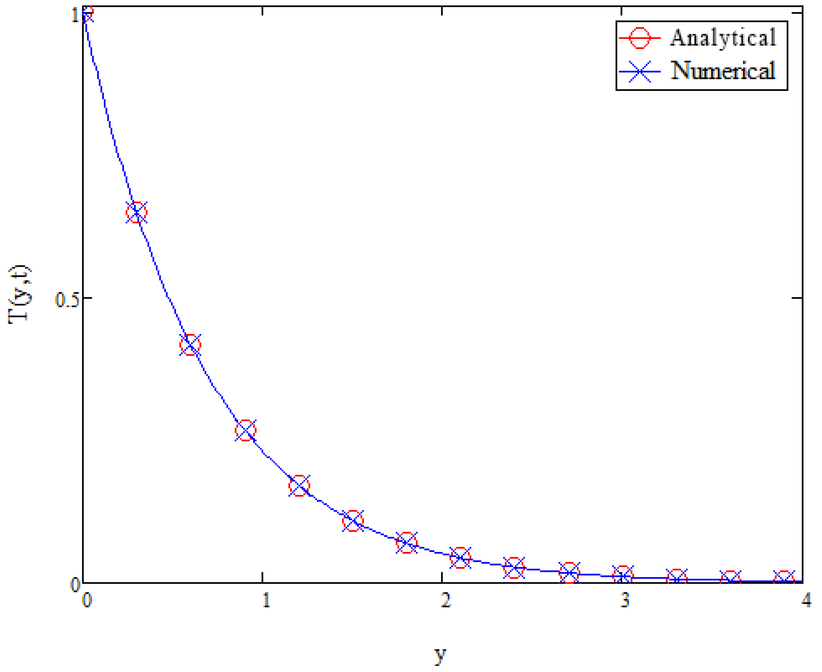
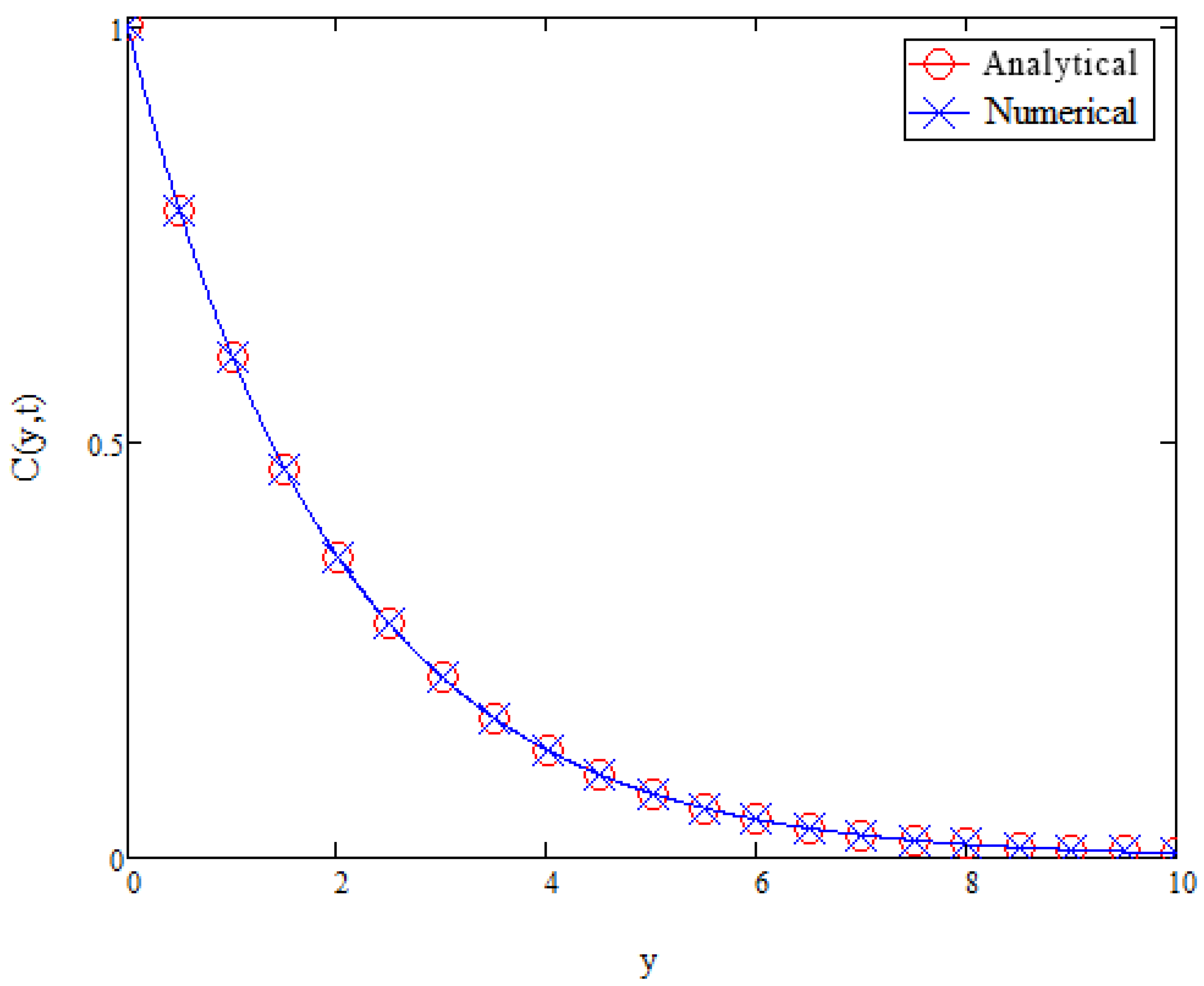
42), respectively, with Mathcad-15. Initially, the solutions were validated by comparing analytical results with semi-analytical results obtained via the Laplace–Zakian method.
Figure 2,
Figure 3 and
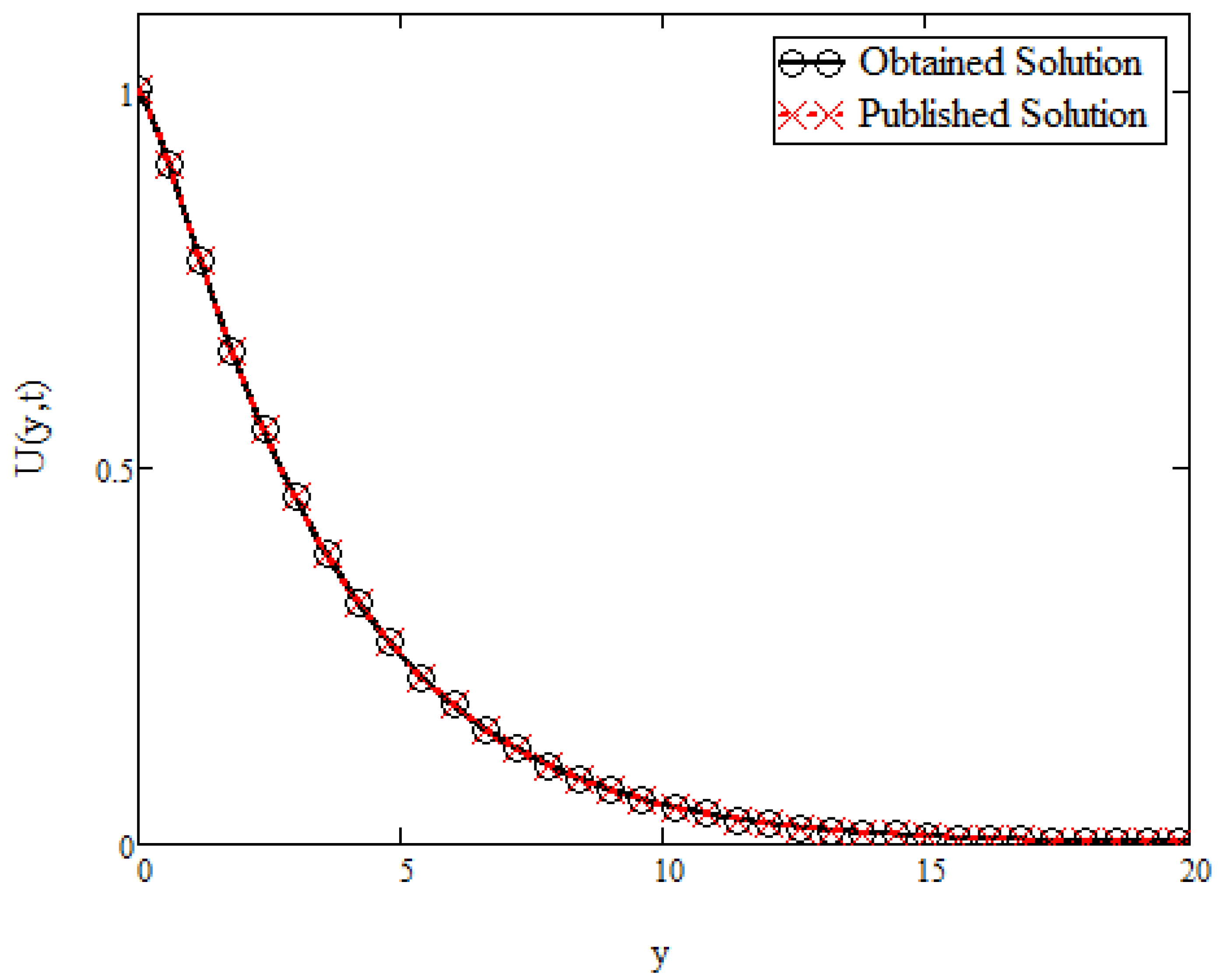
Figure 4 shows the comparison of velocity, temperature, and concentration profiles between the obtained analytical solutions and the semi-analytical solutions. As observed, each of the analytical solutions for each profiles fits perfectly with its corresponding semi-analytical solutions. To further verify the obtained results, a comparison with published limiting case from Ali et al. [
35] was done. The comparison is displayed in
Figure 5. It is observed that the obtained results are in excellent agreement with that of Ali et al. [
35]. Thus, the analytical solutions obtained from this study is accepted and valid.
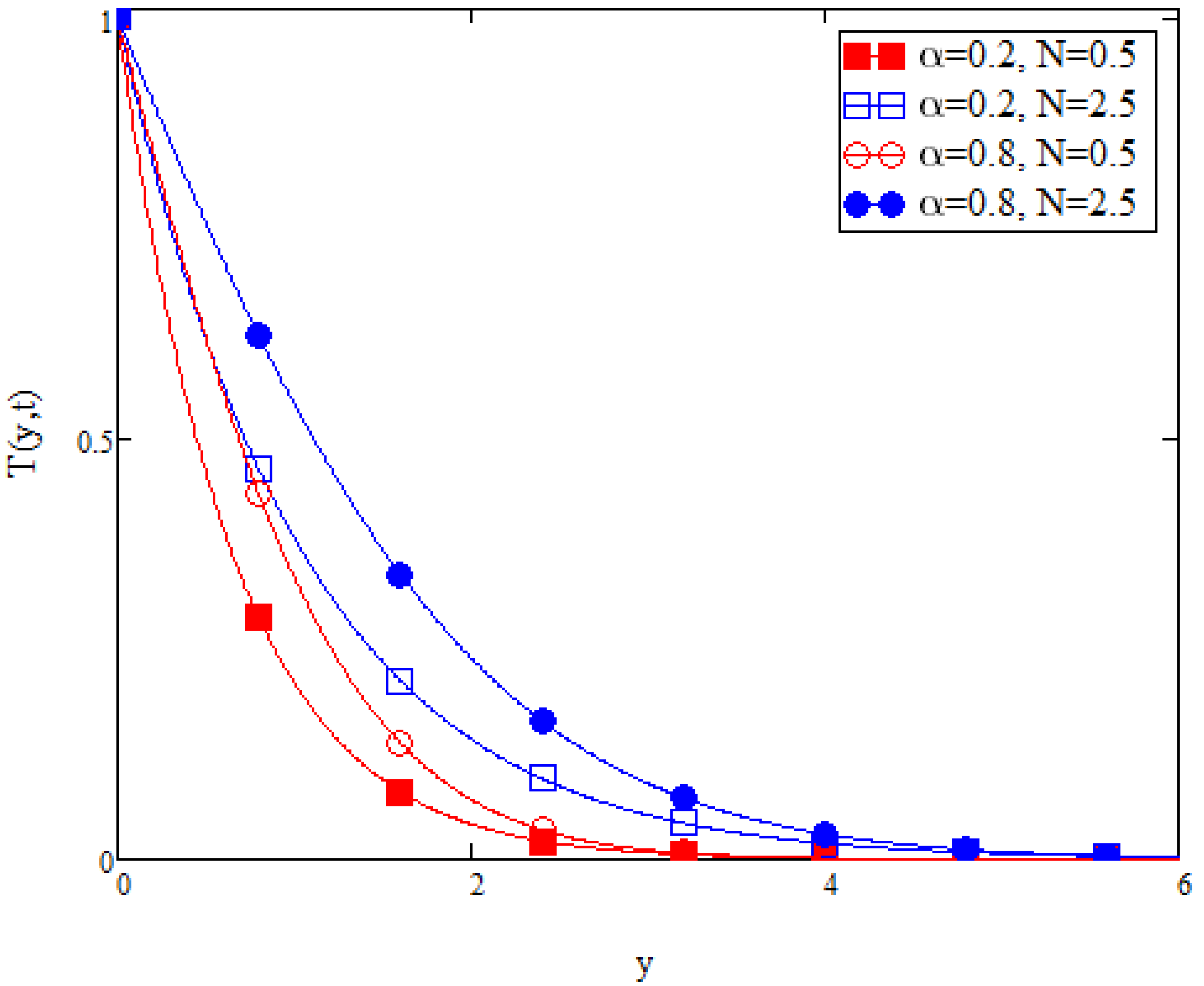
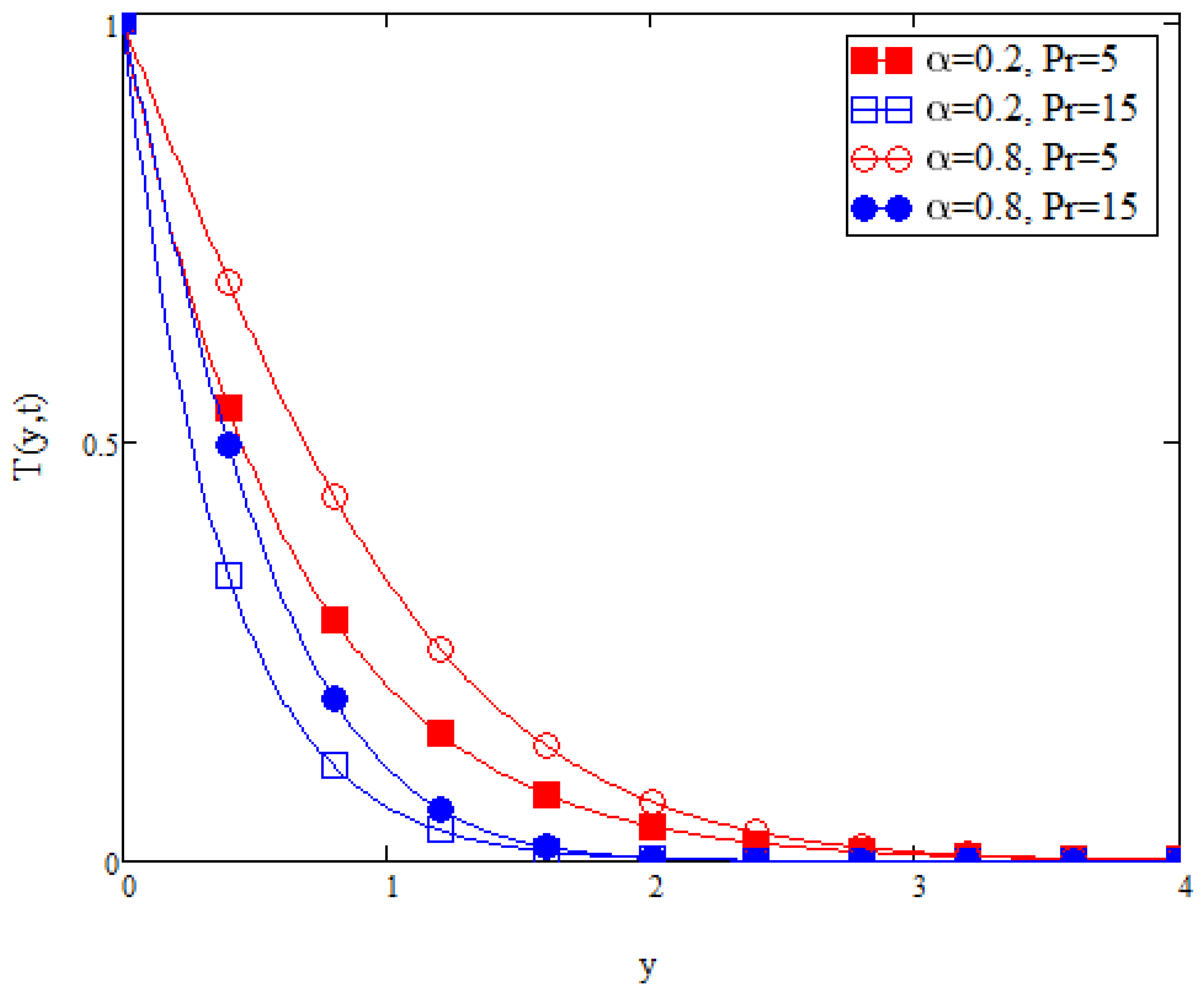
Analysis of obtained results begins with
Figure 6 and
Figure 7. These figures shows the temperature profiles for solutions obtained from Equation (
21) with variations in
N and
Pr, respectively. Both of the figures also show variations in fractional parameter,
. From
Figure 6, it is observed that if the value of
N increases so does the temperature profile. Increasing values of
N indicates increasing amount of thermal radiation applied to the fluid. As the amount of thermal radiation increases, the amount of heat applied to the system is also increased, thus increasing the temperature of fluid. Meanwhile, from
Figure 7, it is observed that the temperature profile decreases as the
Pr value increases. The Prandtl number is defined as the ratio between the diffusivity rate of momentum and diffusivity rate of heat. Hence, the increment of Prandtl number increases the momentum diffusivity and decreases the thermal diffusivity. With a decrease in thermal diffusivity, the amount of heat introduced into the fluid is low, thus the fluid temperature decreases with an increase in the
Pr value. From both,
Figure 6 and
Figure 7, it is shown that the fluid temperature increases as
increases. It is indicated from past literature that the geometrical applications of fractional derivatives has yet to be found. Nonetheless, the behaviour of fluid temperature with variation of
, presented in
Figure 6 and
Figure 7, could be used by experimental researchers to validate their results.
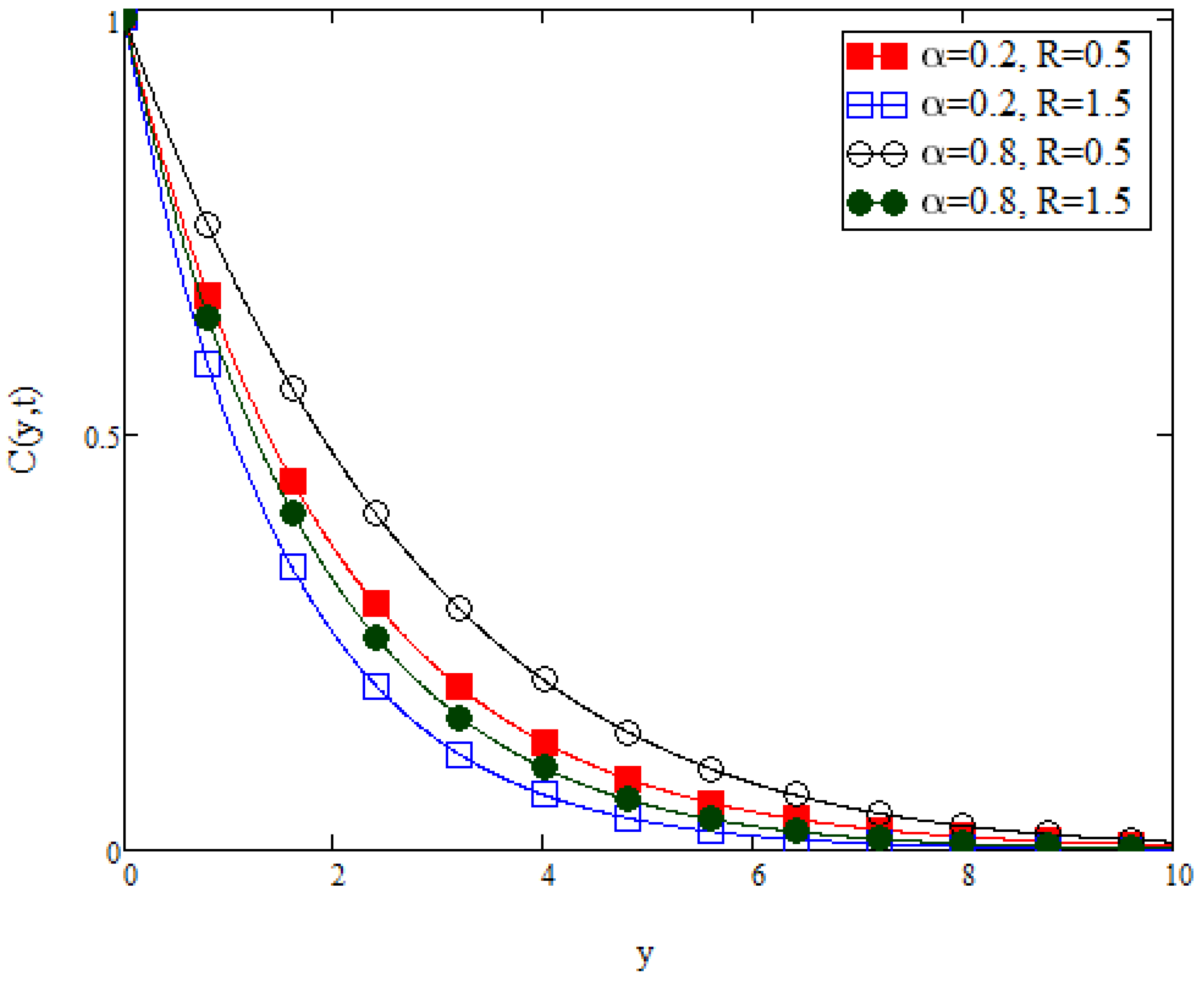
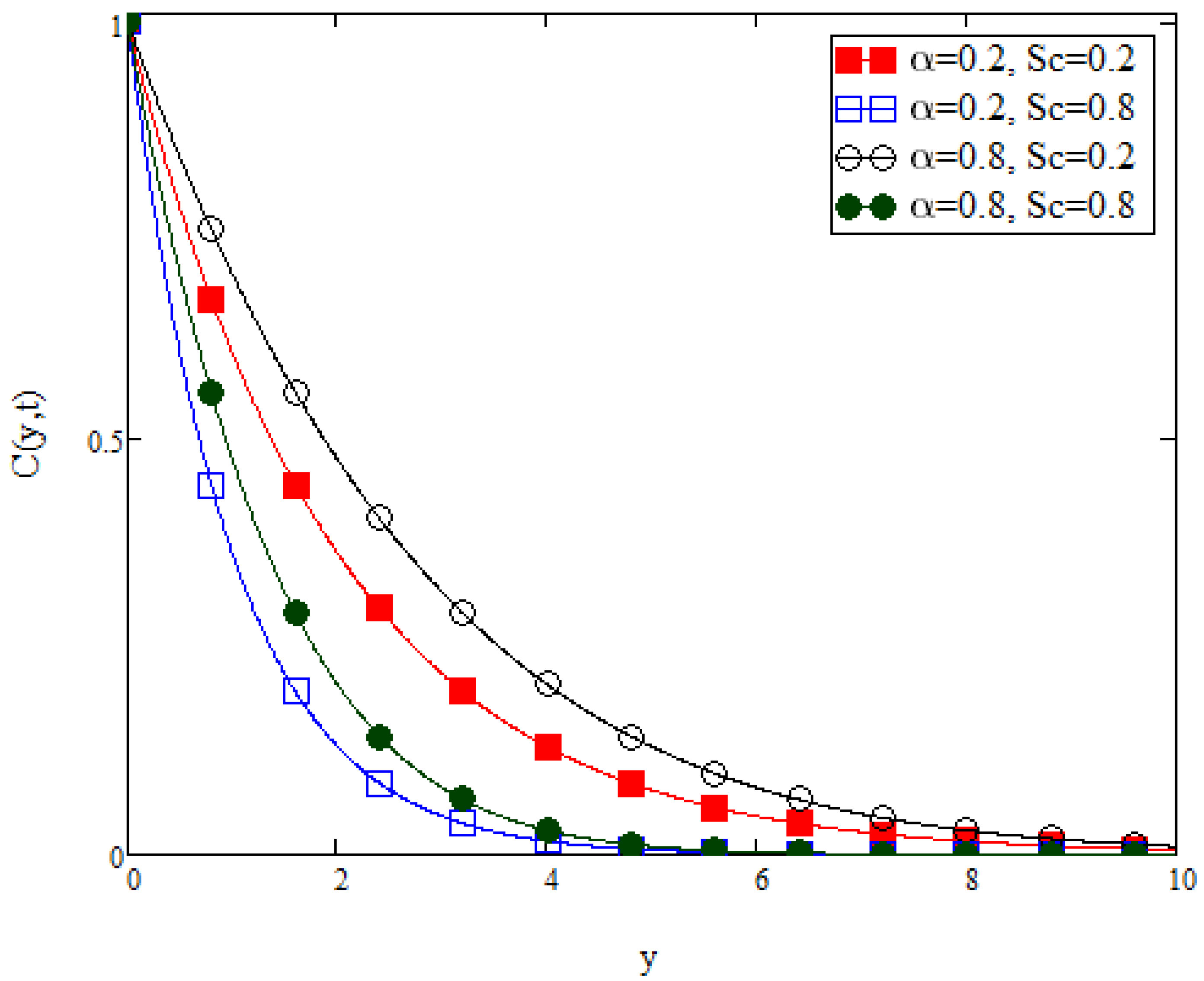
Next,
Figure 8 and
Figure 9 display the concentration profiles obtained from Equation (
22) with variations in
R and
, respectively. Both figures show variations in
as well. It is observed from
Figure 8 that as
R increases, the concentration profile decreases. The chemical reaction rate,
R, determines the species concentration. In this study, a destructive chemical reaction was considered. This is noted by the negative value of the chemical reaction rate parameter,
, in Equation (
3). A destructive chemical reaction tends to create a large disturbance, affecting the species concentration. The larger the chemical reaction rate, the larger the disturbance. The species concentration decreases, at the same time, decreasing the concentration of the fluid. Meanwhile in
Figure 9, it is observed that increasing the
value decreases the concentration profile. The Schmidt number,
, can be described as ratios between the rate of diffusion of momentum or the kinematic viscosity, and the rate of diffusion of the fluid mass. Increasing the
value increases the momentum diffusivity and decreases the mass diffusivity. Thus, with a decrease in the mass diffusivity, the amount of mass introduced into the fluid decreases as well. Consequently, decreasing the concentration of fluid. In both
Figure 8 and
Figure 9, concentration profiles increases as
increases. As mentioned before, this observed behaviour in variation of the fractional parameter,
, could be used in experimental research in the future as a means of validating their results.
Next,
Figure 10,
Figure 11,
Figure 12,
Figure 13,
Figure 14,
Figure 15,
Figure 16,
Figure 17,
Figure 18 and
Figure 19 show velocity profiles with various values of
,
,
,
,
M,
N,
Pr,
R,
, and
t, respectively. Just like the temperature and concentration profiles, each figure from
Figure 10,
Figure 11,
Figure 12,
Figure 13,
Figure 14,
Figure 15,
Figure 16,
Figure 17,
Figure 18 and
Figure 19 show variations in the fractional parameter,
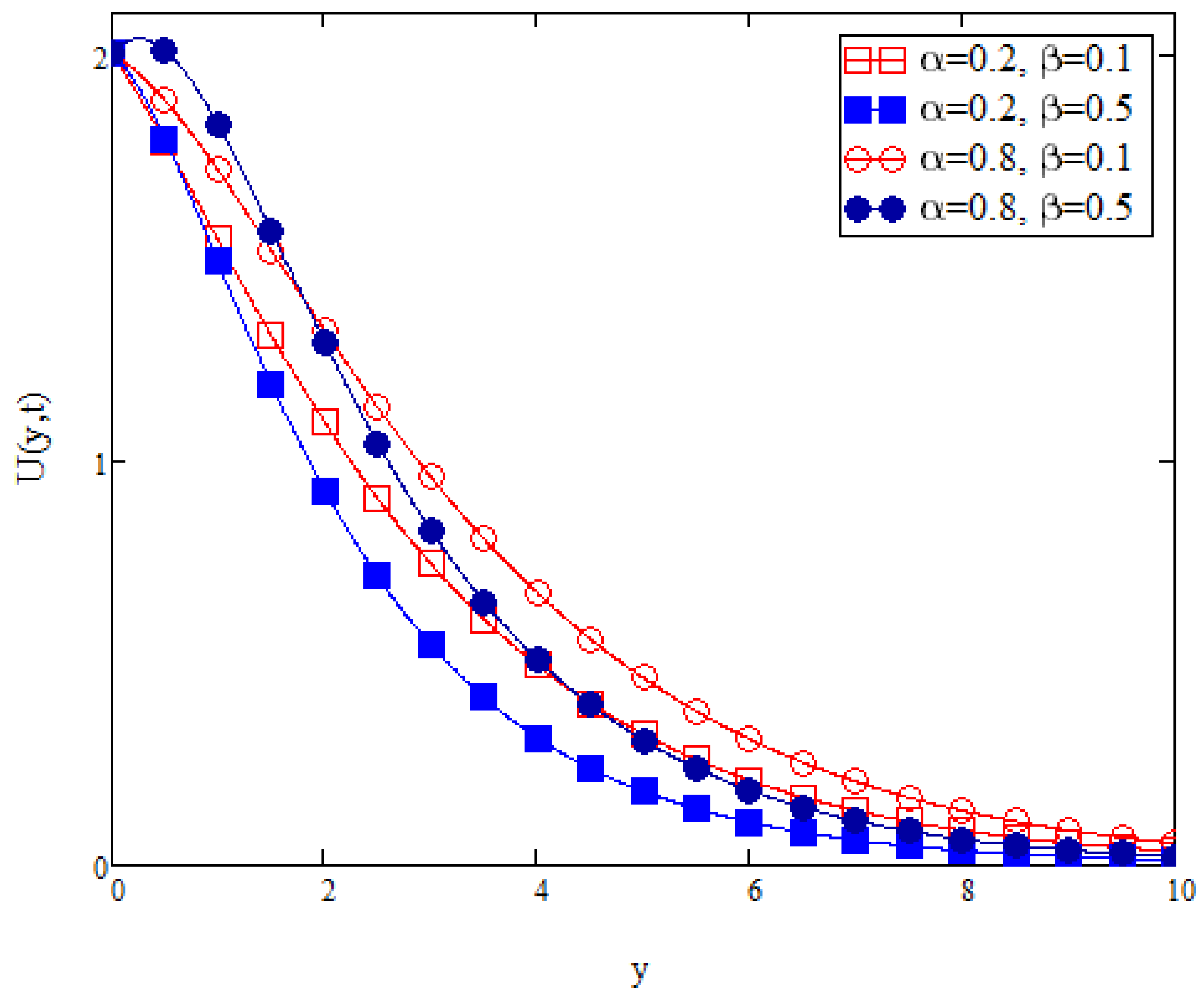
, as well. To begin with,
Figure 10 shows the velocity profile with variation in the Casson parameter,
. A Casson fluid is described as a shear thinning liquid with viscoplastic properties. If the shear rate is less than the yield stress, the fluid would behave as a Newtonian fluid. A fluctuation in fluid behaviour is observed in
Figure 10. Fluid velocity increases with an increase in
. After a certain point on the y-axis, as
increases, viscosity of fluid would also increase and this resulted in the reduction of its velocity. From that point onward, fluid behaves as a non-Newtonian fluid instead of a Newtonian fluid.
Figure 10 also shows that an increase in
resulted in an increase in the fluid velocity.
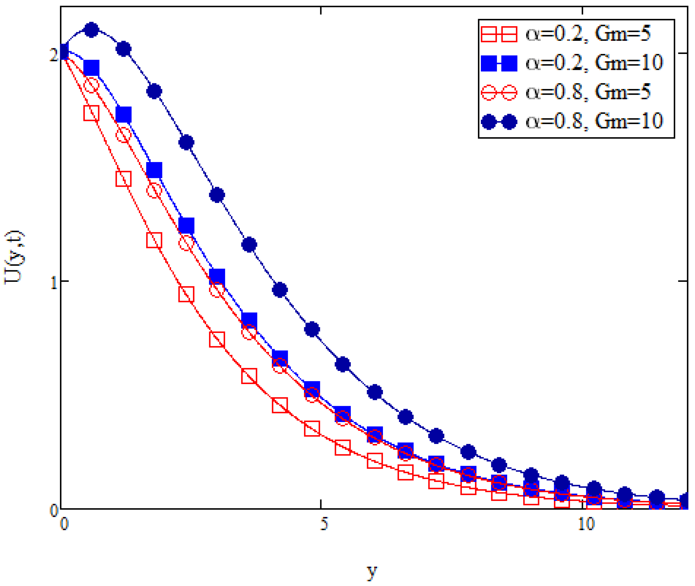
Figure 11 displays the fluid velocity with variation in the mass Grashof number,
. A mass Grashof number is described as the ratio between the buoyancy force and the viscous hydrodynamic force. As the value of
increases, the buoyancy force on the fluid flow increases and the viscous hydrodynamic force decreases. As the fluid flow considered in this study is flowing along a vertical plate, an increase in the buoyancy force would aid the velocity of fluid. Thus, as
increases, the fluid velocity also increases. This behaviour is observed clearly in
Figure 11. In addition in
Figure 11, it is observed that if the fractional parameter,
, is increased, velocity of fluid also increases.
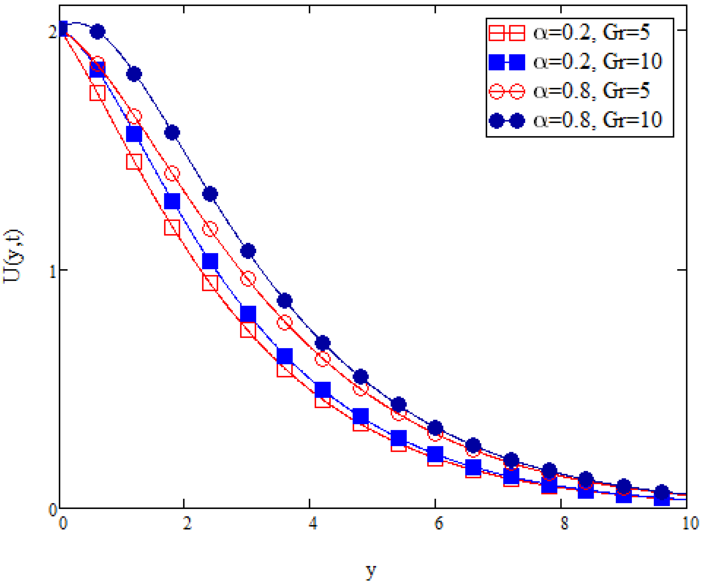
Figure 12 depicts the velocity profile with variation in the thermal Grashof number,
. Similar to the mass Grashof number, a thermal Grashof number is the ratio between the buoyancy force and viscous hydrodynamic force. Unlike the mass Grashof number where the buoyancy force is dependent on the solutal volumetric expansion of the liquid, the buoyancy force of a thermal Grashof number is dependant on the thermal volumetric expansion of the liquid. Thus, increasing the
consequently increases the buoyancy force. However, the increase in the buoyancy force is due to the thermal volumetric expansion, not the solutal volumetric expansion. As mentioned before, since the fluid flow considered is moving along the vertical plate, an increase in the buoyancy force ultimately increases the fluid velocity. It is also observed from
Figure 12 that an increase in the fractional parameter,
, resulted in an increase of the fluid velocity.
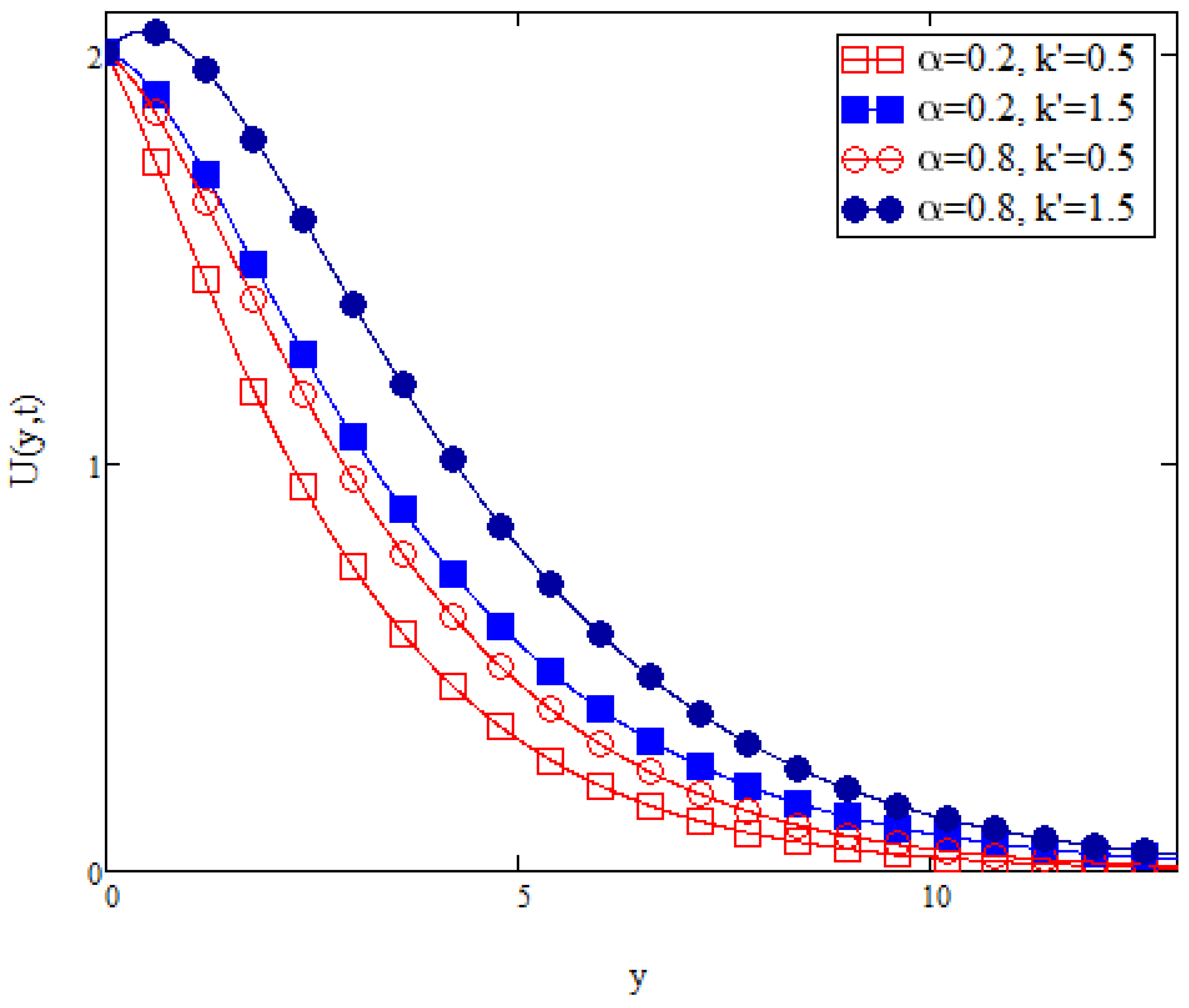
Figure 13 presents the impact of medium porosity,
, on the velocity profile. As the value of
is increased, porosity of medium is also increased, providing more voids, or pores, thus limiting obstacles that produce friction against the fluid flow. Thus velocity of fluid increases with an increase in porous medium parameter
. From
Figure 13, it is observed that an increase in the fractional parameter
, resulted in an increase in the fluid velocity.
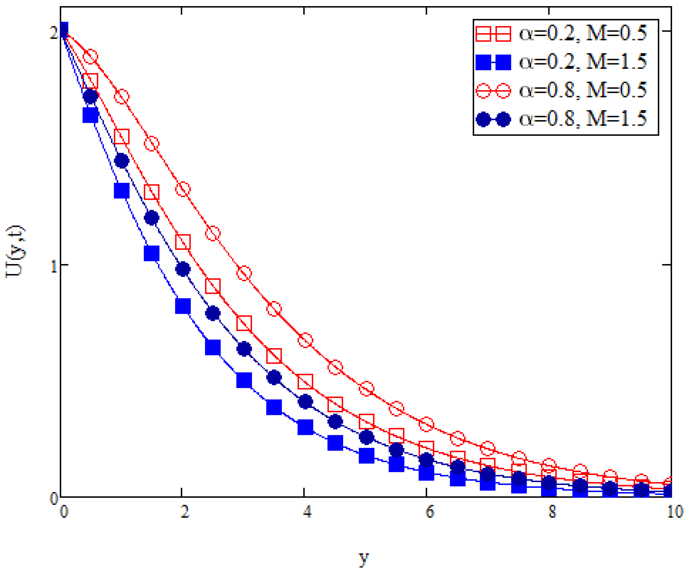
Figure 14 shows the velocity profile with variation in the magnetohydrodynamic (MHD) parameter,
M. Presence of MHD is usually indicated by presence of a magnetic field nearby the fluid flow. The induced magnetic field is possibly due to the presence of a magnetic material or even presence of an electrical current that induces magnetic fields. As the MHD parameter increases, the pulling force from the magnetic field also increases. This in turn hinders the fluid flow, thus decreasing the fluid velocity. Similarly,
Figure 14 shows an increase in fluid velocity with an increase in fractional parameter
.
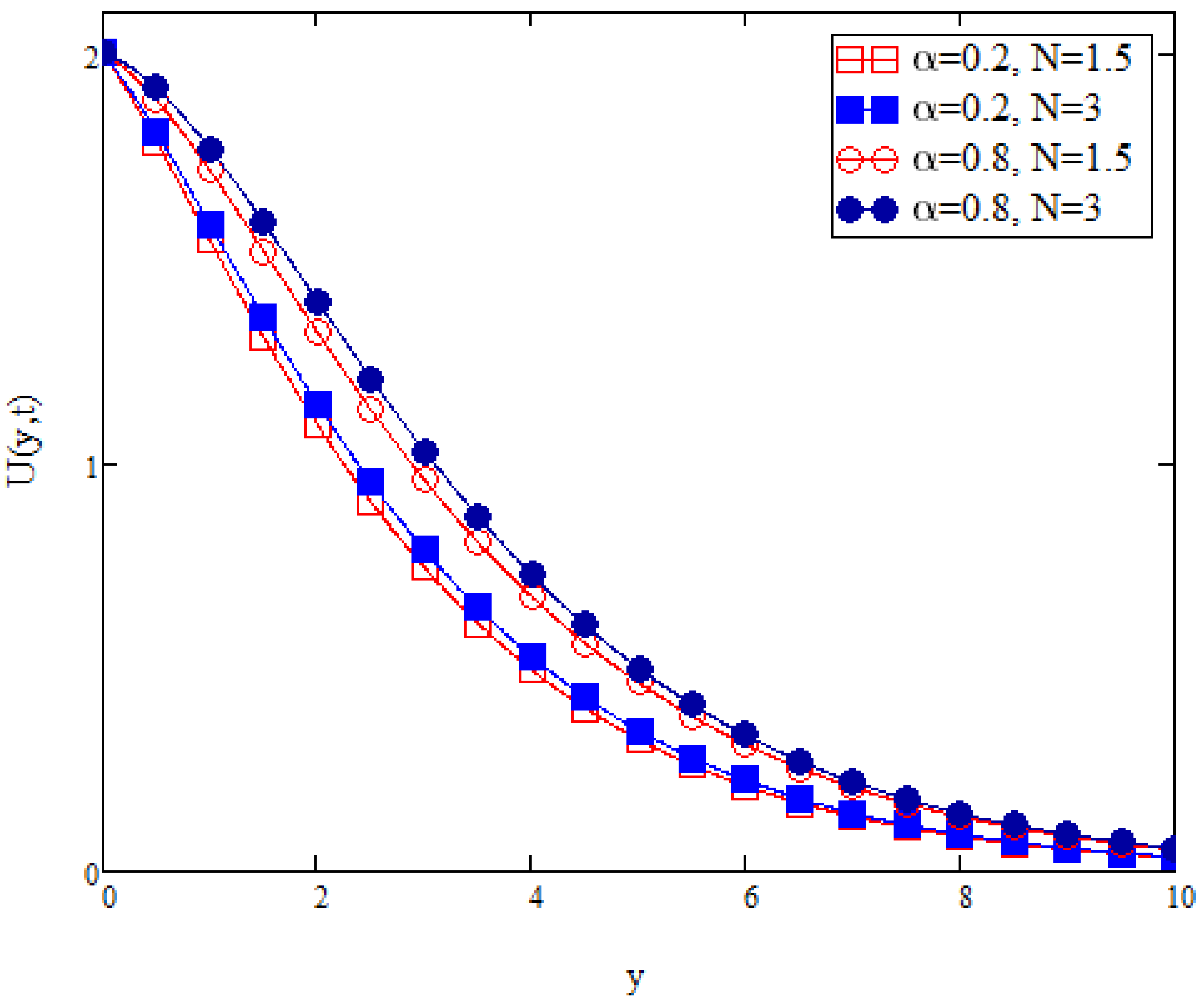
Figure 15 displays the velocity profile with variation in thermal radiation effect,
N. As mentioned, an increase in the thermal radiation ultimately increases the presence of heat in the fluid flow. This in turns increases the kinetic energy of the fluid and velocity of fluid increases. Thus, as observed in
Figure 15, if the value of
N is increased, velocity of fluid also increases. In addition, in
Figure 15, it is observed that an increase in fractional parameter
also increases the fluid velocity.
Figure 16 illustrates the fluid velocity profile with variation in the Prandtl value,
Pr. As mentioned before, an increase in
Pr, increases the momentum diffusivity and decreases the thermal diffusivity. Momentum diffusivity is directly related to an external pressure, the Shear stress, or both. Increasing the momentum diffusivity indicates that an external pressure is applied or the Shear stress is increased. This in turn hinders the fluid flow, decreasing its velocity. Thus, as observed in
Figure 16, the velocity profile decreases when
Pr is increased. From
Figure 16, it is observed that fluid velocity increases with an increase in fractional parameter
.
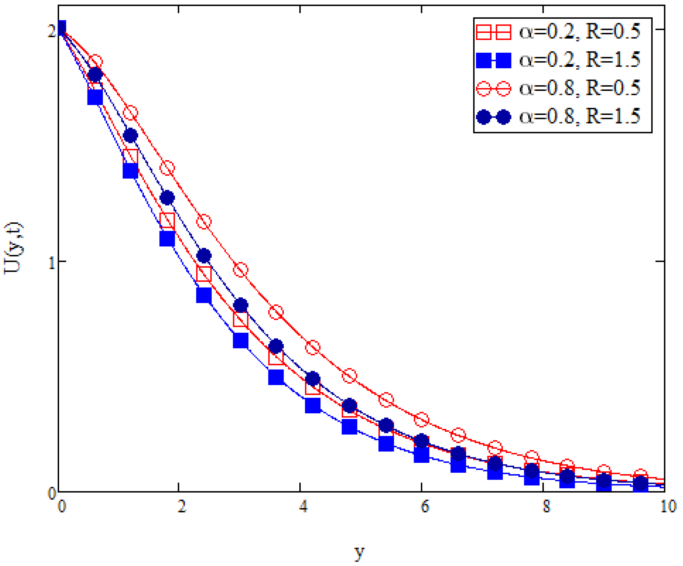
Figure 17 displays the fluid velocity profile with variation in the chemical reaction effect,
R. As mentioned previously, the chemical reaction considered in this study is a destructive chemical reaction. An increase in
R indicates a more active destructive chemical reaction. Since a destructive chemical reaction creates a massive disturbance, fluid flow is indefinitely disrupted. Thus, when the value of
R is increased, the velocity decreases.
Figure 17 also shows that the fluid velocity increases with an increase in fractional parameter
.
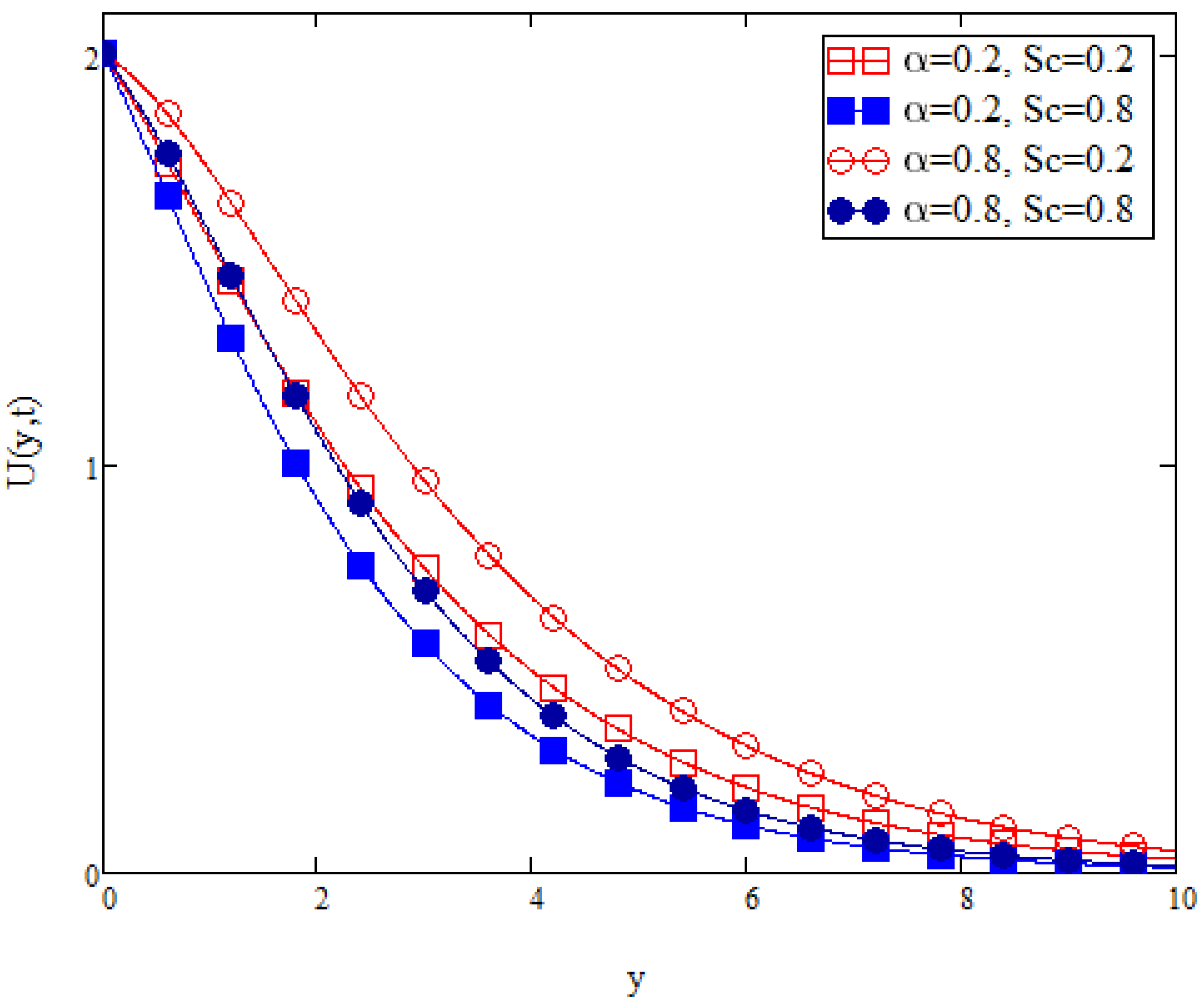
Figure 18 depicts the fluid velocity profile with variation in Schmidt number,
. As mentioned before, the Schmidt number is defined as the ratio of the momentum diffusivity and the mass diffusivity. An increase in the value of
indicates an increase in the momentum diffusivity. An increase in the momentum diffusivity is likely due to an external pressure applied onto the fluid or an increase in the shear stress or both. Either one of these cases could interrupt the flow of fluid. Thus, as observed in
Figure 18, an increase in the value of
decelerates the fluid flow. It also shows that an increase in the fractional parameter
, increases the fluid velocity.
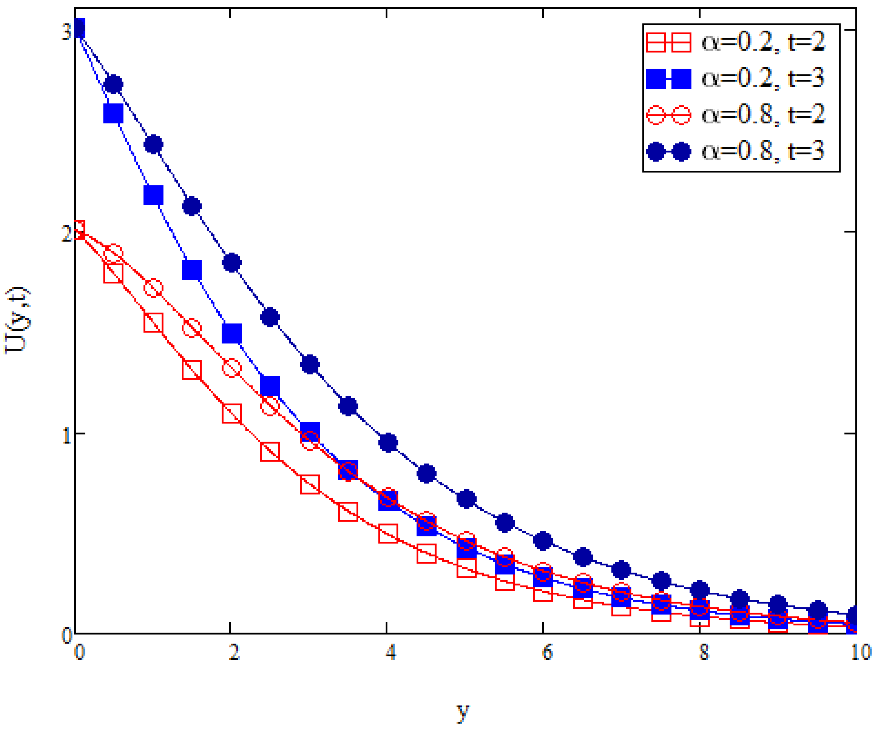
Figure 19 illustrates the fluid velocity profile with variation in time,
t. In this study, it is considered that the fluid is flowing over a vertical uniformly accelerated plate. This in turn creates an initial condition, such as Equation (
4), where initially the velocity of the fluid is at
. Through the process of non-dimensionalisation, the initial velocity is derived as Equation (
10), where the velocity of fluid is initially at
t. Thus, with an increase in
t, the initial velocity of fluid increases as well, satisfying the boundary conditions.
Figure 19 also shows that the fluid velocity increases with an increase in the fractional parameter
.
Aforementioned, based on
Figure 10,
Figure 11,
Figure 12,
Figure 13,
Figure 14,
Figure 15,
Figure 16,
Figure 17,
Figure 18 and
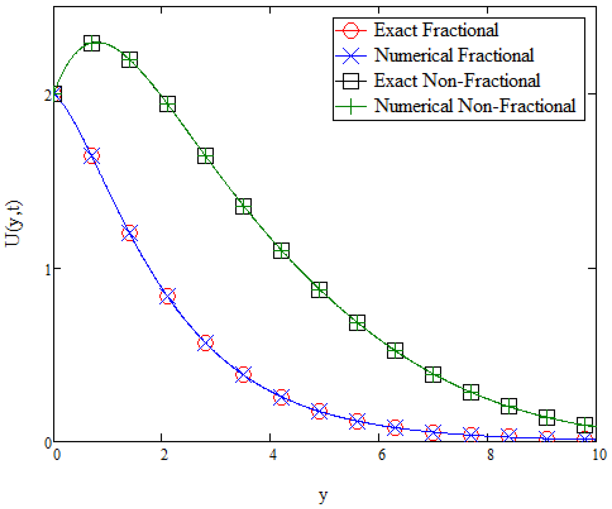
Figure 19, it is observed that the velocity profile increases with the increment of
. To further investigate the impact of fractional derivatives on an MHD Casson fluid flowing over an accelerated plate, a comparison between the fractional derivative solution, from Equation (
20) and a classical, non-fractional, derivative solution, from Equation (
30), were conducted. Analysis of this comparison is displayed in
Figure 20. It is shown that the non-fractional solution produces a velocity profile that is higher than the fractional solution. Observing the pattern of an increasing fractional parameter from
Figure 10,
Figure 11,
Figure 12,
Figure 13,
Figure 14,
Figure 15,
Figure 16,
Figure 17,
Figure 18 and
Figure 19 as well as
Figure 20, it can be suggested that higher values of fractional derivative parameter provide solutions that achieve steady state later compared to a lower values of the fractional parameter. Thus, it can be inferred that fractional parameters arising from fractional derivatives do have an impact on the velocity of a fluid. Although there is yet a geometrical application of fractional derivatives in the field of fluid flow, obtained solutions will be useful in validating experimental studies that will be carried out in the future.
Figure 20 also illustrates analytical solutions for both velocity profiles, with and without fractional derivatives, that is plotted against their respective semi-analytical solutions to be validated. Henceforth, both solutions are valid since they fit perfectly with their corresponding semi-analytical solutions.
Table 1,
Table 2 and
Table 3 displays the Nusselt number, Sherwood number, and skin friction of the fluid flow with variations in the parametric values. From
Table 1 it is observed that the Nusselt number increases with increment in
Pr but decreases with increment in
and
N. The Nusselt number is defined as the ratio between the convective heat transfer and the conductive heat transfer. Increasing the Prandtl value resulted in the reduction of the thermal diffusion. This causes the conductive heat transfer in the fluid to be lowered and therefore increasing the Nusselt number value. This is the opposite when raising the thermal radiation value,
N. Increasing the value of
N would ultimately increases the temperature of the fluid, thus increasing the conductive heat transfer and consequently reducing the Nusselt number value. From
Table 2, it is observed that the Sherwood number increases as the values of
and
R increases but decreases as
increases. The Sherwood number is described as the ratio between the convective mass transfer and the diffusivity of mass. Increasing the Schmidt value resulted in the reduction of the mass diffusivity, coherently increasing the Sherwood number. Similarly, increasing the chemical reaction rate,
R, would cause an increase in the mass convection rate, thus increasing the Sherwood number.
Table 3 shows that the skin friction increases with the increment of
Pr,
,
R, and
M, but decreases with the increment of
,
,
,
,
N, and
. The skin friction value is the result of frictional shear force exerted to the fluid parallel to the flow. A higher skin friction value is the result of a higher drag force created from the friction of the plate surface. According to
Figure 10,
Figure 11,
Figure 12,
Figure 13,
Figure 14,
Figure 15,
Figure 16,
Figure 17,
Figure 18 and
Figure 19, higher values of
Pr,
,
R, and
M resulted in lower fluid velocity, while higher values of
,
,
,
,
N, and
resulted in a higher fluid velocity. This reflects excellently on the result of skin friction, where lower fluid velocities have higher skin friction and higher fluid velocities have lower skin friction.


 ,
, 


