
Fractional Differential Equation-Based Instantaneous Frequency Estimation for Signal Reconstruction


Department of Electrics and Electronics, Istanbul Technical University, Istanbul 34469, Turkey
*
Author to whom correspondence should be addressed.
Fractal Fract. 2021, 5(3), 83; https://doi.org/10.3390/fractalfract5030083
Submission received: 1 July 2021
/
Revised: 26 July 2021
/
Accepted: 27 July 2021
/
Published: 30 July 2021
(This article belongs to the Special Issue Fractional Behavior in Nature 2021)
Abstract
:In this paper, we propose a fractional differential equation (FDE)-based approach for the estimation of instantaneous frequencies for windowed signals as a part of signal reconstruction. This approach is based on modeling bandpass filter results around the peaks of a windowed signal as fractional differential equations and linking differ-integrator parameters, thereby determining the long-range dependence on estimated instantaneous frequencies. We investigated the performance of the proposed approach with two evaluation measures and compared it to a benchmark noniterative signal reconstruction method (SPSI). The comparison was provided with different overlap parameters to investigate the performance of the proposed model concerning resolution. An additional comparison was provided by applying the proposed method and benchmark method outputs to iterative signal reconstruction algorithms. The proposed FDE method received better evaluation results in high resolution for the noniterative case and comparable results with SPSI with an increasing iteration number of iterative methods, regardless of the overlap parameter.
1. Introduction
Signal reconstruction from short-term Fourier transform (STFT) magnitude spectra is a topic that never loses its relevance. This subject, also referred to as the phase recovery problem or spectrogram inversion problem, has attracted the attention of various researchers, and important studies have been carried out. The most-used approach for solving this problem is the well-known Griffin–Lim algorithm (GLA), which was first introduced by Griffin and Lim as an iterative repetition of inverse STFT (ISTFT) and STFT by considering initial phase conditions and exploiting the property of spectrogram redundancy [1].
As the GLA and its derivatives are iterative algorithms, they are time consuming [2,3]. Therefore, in areas where application speed is a concern, different algorithms have been proposed such as single-pass spectrogram inversion (SPSI). SPSI not only outputs applicable results, but also provides a better initial phase estimate for iterative methods such as the GLA [4]. Recently, various methods were proposed for noniterative signal reconstruction problems that claimed improved results concerning SPSI [5,6]. Moreover, with the emergence of deep learning, neural models have produced state-of-the-art results [7,8,9,10]. As a common rule, all recent methods provided results in comparison with SPSI, thus solidifying its place as a benchmark [11].
Historically, phase recovery methods have been model-based approaches. Speech and musical signals, which are defined as semi-stationary signals, have been represented with sinusoidal models. A sinusoidal model takes a speech signal of a given frame length, the time length in which the audio signal is accepted as stationary, as a weighted sum of sinusoids with different phases, frequencies, and amplitudes [12]. The sinusoidal model has been used in both analysis and synthesis applications of audio signal processing. Phase vocoder applications are used for audio signal synthesis for audio processing applications [13]. During synthesis, a given encoded audio signal or a feature set of an audio signal is used to reconstruct the signal in the time domain. Generally, short-term Fourier transform (STFT) magnitudes are analyzed to define phase and frequency components of sinusoids.
For example, the SPSI algorithm first detects spectral peaks and applies quadratic interpolation techniques around the neighborhood of peak bins to obtain an estimate for instantaneous frequency. First, the magnitude of the STFT of the signal is calculated; then, a quadratic function that passes through an amplitude point at peak bin and amplitude points in its two neighborhoods is fitted [14]. Next, with the phase-locked vocoder approach, signal phases are obtained. A linear interpolation gives the phase estimate, which is called the phase accumulator. In the frequency domain, if a peak has happened, a simple estimate for phases of its adjacent bins is a 180° shift. If the peak is not in the center but between two peak bins, it is assumed that one of the adjacent bins also influenced the phase. Therefore, a phase alternation strategy dependent on the location of the instantaneous frequency estimate was proposed [15].
In signal synthesis, there are model assumptions that signals typically obey, such as them being sinusoids or them being solutions to ordinary differential equations (ODEs). For calculating the parameters of signals, functions are fitted based on these assumptions. Modeling bandpass filter outputs using ODEs have found use in sound synthesis [16]. Using simple time-dependent and nonlinear terms, the relationship between ODE coefficients and physically meaningful control parameters such as pitch, pitch bend, decay rate, and attack time can be stated. This relationship makes it possible to generate artificial sounds using ODE models. One of the assumptions for signal models is that a signal is a result of the weighted sum of its history. This approach is called linear prediction and it has been widely used in audio signal processing and time-series analysis [17]. This autoregressive approach can be considered as a special case for the more general autoregressive fractionally integrated moving average (ARFIMA), which is used in time-series analysis with signals that show long-term dependence [18]. This property is elemental in fractional-order calculus.
Fractional-order calculus is a generalization of integer order differentiation and integration. The idea of a fractional-order derivative was first discussed by Leibniz and L’Hospital [19]. The mathematical phenomena of fractional-order calculus make it possible to describe real objects more accurately than classical, integer order calculus. Due to the extra free parameter of the non-integer derivation order, fractional-order-based methods provide an additional degree of freedom in modeling objects, optimizing performance, and describing natural dynamical behavior with memory [20]. Due to these capabilities, the fractional-order calculus framework has a close connection to the theory of fractals. Mandelbrot introduced the concept of fractal theory as a mathematical framework for explaining self-similar structures in nature [21]. Fractal geometry can be translated as the study of textural information, which is important for understanding signals. For example, when assuming that a stochastic signal obeys a well-defined fractal model, a method for estimating the frequency characteristics of a signal can be derived. Moreover, the parameters of this model can be applied to the textural segmentation of a signal [22]. In signal processing, regardless of a signal being fractal or not, fractal theory helps to explain the local properties of a signal and provides a simpler geometrical or statistical description of these properties [23].
Fractional differentiation, or, more correctly, the differ-integration order of a differential equation, gives a metric for the long-term dependence or fractal dimension. Moreover, Grünwald–Letnikow fractional differ-integration shifts a sinusoid phase with direct relation to its differ-integration order [24]. Fractional-order calculus-based models have found use in two ways. First, by differ-integrating a signal, its autocorrelation function can be manipulated. This can result in a reduced number of parameters in linear predictive analysis. An approach based on a weighted sum of fractional derivatives of a signal, which is called fractional linear prediction, has been shown to have good signal prediction capability [25]. Fractional calculus is a nonlocal approach and, therefore, employs infinite memory. Proposed methods for optimal fractional linear prediction with limited memory have not only provided good results on prediction accuracy but also provided a tool for reducing the number of linear prediction coefficients that are needed for encoding an audio signal [26,27,28]. Another application of the fractional derivative in audio processing is using it as a metric for fractal analysis. The excitation in an autoregressive model can be assumed as the fractional derivative of Gaussian noise [29]. Fractal features have also been applied to speech recognition, voiced–unvoiced speech separation [30], and speaker emotion classification [31]. A fusion of fractal-geometry-based features was shown to produce comparable results to mel-frequency cepstral coefficients when applied to speech classification problems [32].
In this article, the fractional-order calculus framework is applied to the audio reconstruction problem, whereby bandpass filter outputs around peak frequencies are modeled as fractional-order differential equations. Fractal geometry or fractional-order calculus-based models have been applied to various cases of signal processing to an extent, but we show that this framework has higher potential by linking the memory feature of the fractionally integrated model to instantaneous frequency estimates. Our starting point is simple. A signal with long-range dependence is expected to show low-frequency behavior, and a signal without long-range dependence is expected to show high-frequency behavior. By analyzing a signal’s long-range dependence, we can create a model to estimate its instantaneous frequency. Furthermore, by applying this framework to the phase reconstruction problem, we show that a method based on a fractional-order differential equation model can achieve better objective test scores using the perceptual evaluation method than the benchmark SPSI method in redundant conditions. We compared our results with those of three different GLA-based methods and show that our proposed phase reconstruction method produces similar results to the benchmark.
2. Materials and Methods
In time-series applications or fractal theory, the use of differential equations is valid and has many applications. In time-series analysis, an ARFIMA (0, d, 0) process with unit increments of time index t can be generalized as a fractional differential equation [33].
In Equation (1), the f(t) signal is a one-dimensional vector with a length of T. Most audio processing applications deal with normalized and sampled signals with respect to the specified sample rate. To avoid dependence on the sample rate and reaching physically incorrect models, we take f(t) as a dimensionless signal, and t as a dimensionless variable of time [22]. The power spectral density function (PSDF) of is given by , and is white noise. The PSD of white noise is a constant c; hence, the following equation is valid:
The PSD of a function, modeled as a fractional differential equation, can be estimated as
where .
From Equation (3), we can see that, depending on the value of , the system exhibits different characteristics in terms of long-range dependence and frequency response.
If 0, the system in Equation (3) becomes a differentiator. The spectrogram of the system will be dominated by high-frequency components as the differentiator behaves like a high-pass filter. Consequently, the system will not exhibit long-range dependence.
If 0, the system in Equation (3) becomes an integrator. The spectrogram of the system will be dominated by low-frequency components as the integrator behaves as a low-pass filter. Consequently, the system will have long-range dependence.
The estimation of differential equation order has been investigated in time-series analyses. One of the most extensively used solutions is a linear regression model, as proposed by Geweke and Porter-Hudak [34]. We can apply the least-squares error method to obtain estimates for and C and create a regression line.
where .
This method is simple to implement. We only need spectrogram magnitudes to evaluate the result, as often is the case with signal reconstruction. If we apply this method to appropriately normalized values, we can reduce the significant workload of least-squares estimation.
To find the values of C and , which minimize this error function, we calculate and . Solving these two equations yields the following expressions for and :
Using Equations (5) and (6), we can estimate
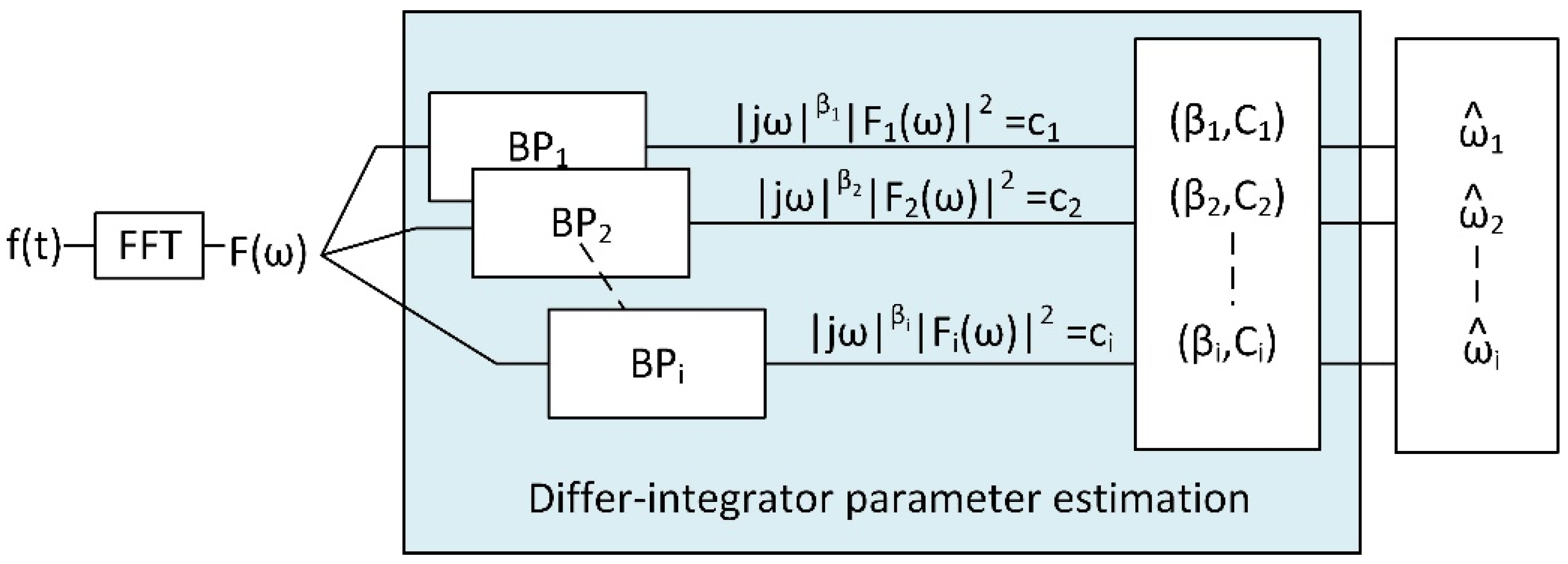
We can use this approach with the modifications described below to estimate instantaneous frequency. Figure 1 shows a diagram of the proposed approach.
First of all, we take spectral peaks and their two adjacent points in the spectrogram into consideration; then, for every peak bin index j, we model these data points according to the differential equation in Equation (1) and obtain their PSDFs as
Equation (8) models PSDF of ith band pass filter output that corresponds to a peak bin index j of a signal frame m. Accordingly, we can create an estimate for new using Equations (3) and (7) as
Then, we can calculate the and values to produce a regression line that passes through the peak and its adjacent points as seen in. Algorithm 1 shows this process.
| Algorithm 1. Pseudocode for FDE-based instantaneous frequency estimation on a signal frame. | |||
| Input: Spectrogram magnitude of the signal frame , NFFT | |||
| Output:, | |||
| 1: | Calculate logarithmic power spectrogram | ||
| 2: | Assign 0.5, 1, 2, 3 to , , , and N | ||
| 3: | |||
| 4: | |||
| 5: | |||
| 6: | |||
| 7: | |||
| 8: | for every spectral peak bin j in do: | ||
| 9: | |||
| 10: | |||
| 11: | if then: | ||
| 12: | |||
| 13: | |||
| 14: | |||
| 15: | |||
| 16: | |||
| 17: | |||
| 18: | else if then: | ||
| 19: | |||
| 20: | |||
| 21: | |||
| 22: | |||
| 23: | |||
| 24: | |||
| 25: | else: | ||
| 26: | |||
| 27: | |||
| 28: | |||
| 29: | |||
| 30: | |||
| 31: | |||
| 32: | endif | ||
| 33: | |||
| 34: | return , sign() | ||
| 35: | endfor | ||
However, we also apply two modifications, as seen in the proposed algorithm. Firstly, we normalize values of 3 points between 0 and 1; secondly, we take constant values for , , and as 0.5, 1, and 2. With these two normalization processes, we end up obtaining linearized frequency indices around the origin and more distributed data points. Moreover, because we have normalized frequency values, we expect that the fractional differentiation order corresponds to the slope of the tangent line. Furthermore, by normalizing frequency values, we force the equation to be in coherence with the theory in [34], which employs a least-squares estimator of the slope parameter in linear regression, formed using only the lowest-frequency ordinates of the log periodogram. Lastly, these predefined values help reduce computational costs.
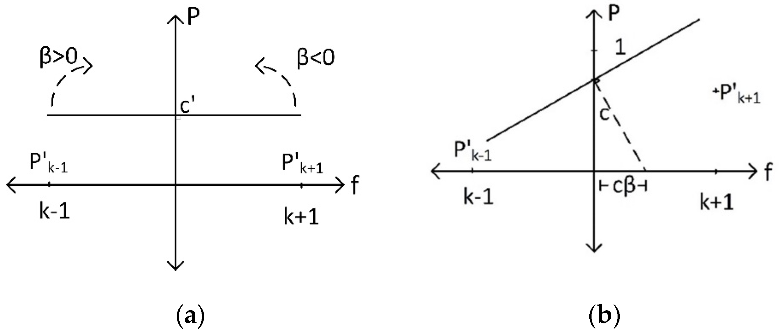
After the calculation of the regression line, two cases are present. Figure 2a,b show these two cases. In case a, we have 0, and, in case b, we have 0. The sign of the value shows whether the frequency for the actual peak is on the left- or right-hand side of the plane. If 0, then we have a system that did not exhibit long-range dependence; therefore, the spectrogram of the system will be populated by a high-frequency component and the regression line will be an increasing line that indicates instantaneous frequency is on the right-hand side of the plane. If 0, we can concur that the system exhibits long-range dependence and, being an integrator, its spectrogram will be populated by low-frequency components. Similarly to case a, we can evaluate that the instantaneous frequency is on the left-hand side of the plane because it creates a decreasing line.
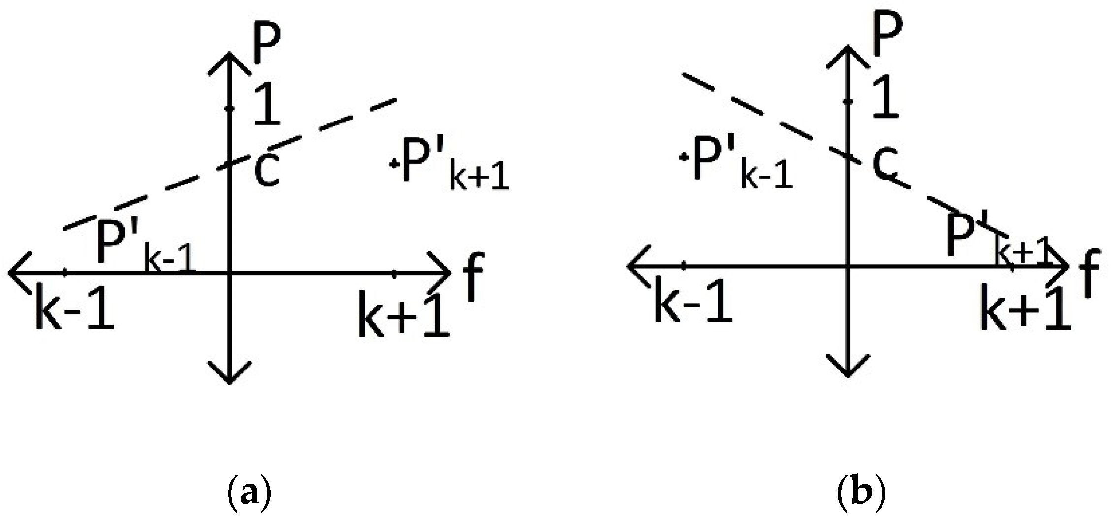
To estimate instantaneous frequency, we calculate the line that is normal to the regression line at the point . The frequency estimate of the model is the value that the normal line hits the x-axis in the frequency domain. This assumption is based on the case of a peak having equally valued adjacent points. In that case, after normalization of and , values are equal to 0 and ; therefore, there is no increasing or decreasing trend. As seen in Figure 3a, the regression line becomes orthogonal to the magnitude axis, indicating that instantaneous frequency was indeed at index k.
In Figure 3b, if 0, the normal line will hit the x-axis at on the right-hand side of the plane. This indicates a new instantaneous frequency estimate. Instantaneous frequency can be calculated as follows:
where NFFT is the size of the fast Fourier transform (FFT) window applied to the signal frame, and j is the frequency index of the spectral peak.
From now on, we can apply the same approaches proposed by Dolson and Puckette to estimate phase values for frames and frequency bins, similarly to SPSI.
Phase values for frequency bin j and frame m can be given as
From [15], we know that phase values for adjacent bins of the peak can be estimated as 180° ()-shifted values. Depending on the sign of , we apply the same scenario as used in SPSI because the instantaneous frequency estimate stays halfway between the peak and adjacent frequency bins. Depending on the value, the weight of the adjacent frequency bins on the phase will change. Thus, if 0, the neighbor bin on the right will also influence the phase; accordingly, bins on the right will have the phase value of the peak bin, and bins on the left will have the -shifted value of the peak bin. If 0, the complete opposite would apply.
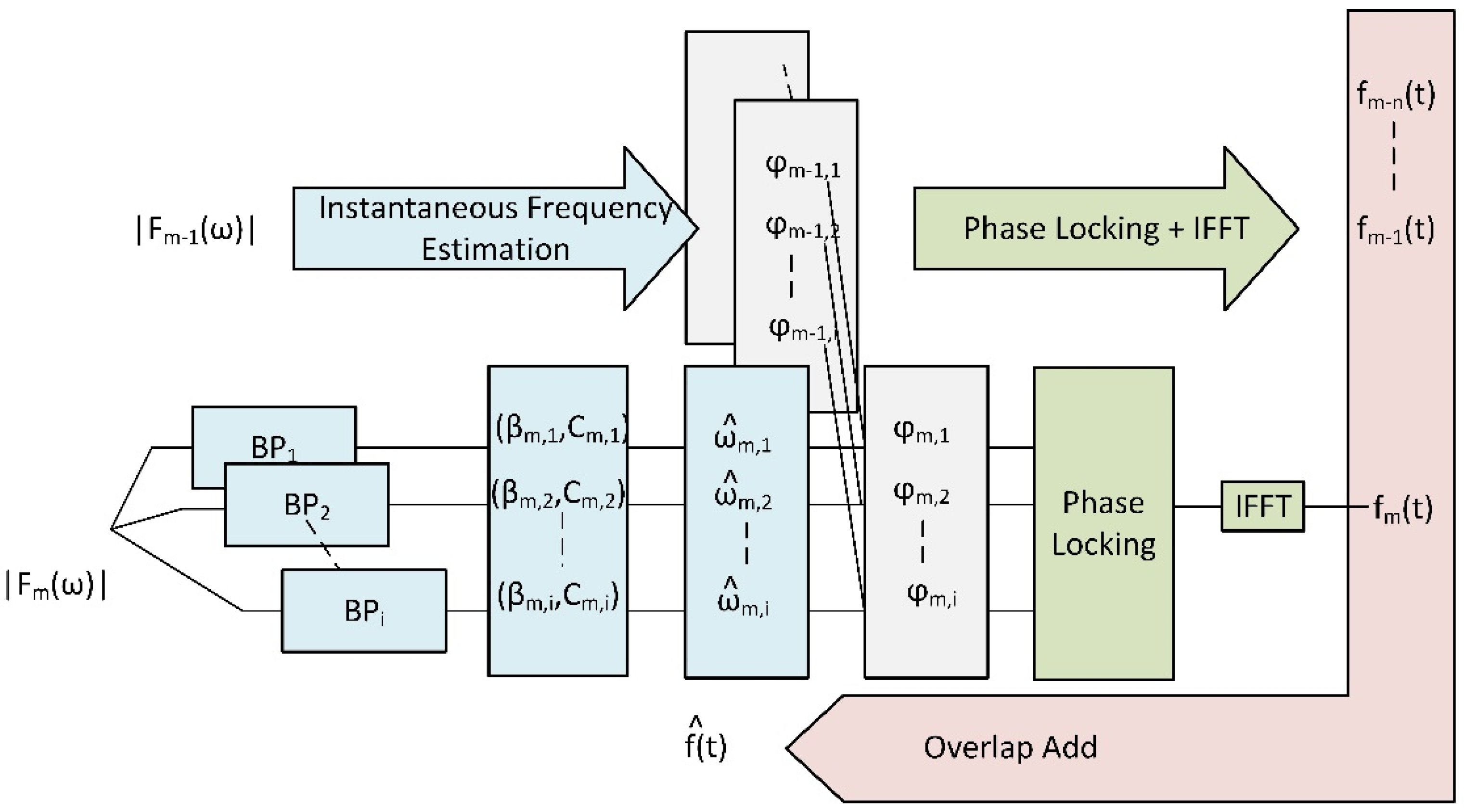
When all the phase values have been computed, the function will return to the time domain by applying inverse FFT (IFFT) with the Hanning window. Then, the frames will be added in an overlapping manner to finally reconstruct the signal. The whole process is summarized in Figure 4.
3. Results
For the tests, we used a subset of the TIMIT database. TIMIT is a read speech corpus, which is used for benchmarking speech processing implementations [35]. The corpus contains 16 bit, 16 kHz speech samples from various dialects of American English. In this work, we used 50 male and 50 female speech samples.
Reconstruction performance was evaluated by two objective measures: spectral convergence (SC) [2] and perceptual evaluation of speech quality (PESQ) [36]. Spectral convergence is commonly used as a loss function or an objective measure and can be given as
In Equation (12), is the target magnitude spectrogram, x is the signal, and denotes the Frobenius norm. This measure is generally used in the logarithmic form . It is widely stated that spectral convergence is not a measure highly correlated with human perception. The perceptual evaluation of speech quality metric was proposed by the International Telecommunication Union Telecommunication Standardization Sector (ITU-T) for providing a highly correlated measure with subjective evaluation metrics. PESQ employs auditory transform that reflects human auditory perceptions, thereby producing highly correlated results with subjective evaluation methodologies such as mean opinion score (MOS) and Multiple Stimuli with Hidden Reference and Anchor (MUSHRA) for 16 kHz sampled data.
A well-known property of the STFT spectrogram is that it is a redundant representation because it is computed by overlapping windowed short-term frames of a signal. This means that there is no guarantee of any spectrogram-like complex number array being equal to the STFT of a signal in the time domain. A complex-valued array that corresponds to the STFT of a time-domain signal is called a consistent spectrogram [37]. Spectrogram consistency is an integral part of signal reconstruction algorithms such as Griffin–Lim. In this regard, overlap value is important because it affects spectrogram resolution and consistency. An increased hop factor also increases aliasing. In the tests, 512 sample length Hamming windows with three different hop sizes of 64, 128, and 256 were applied to the signals. The FDE-based method was compared to SPSI and random phase.
3.1. Comparison of FDE-Based Method to SPSI with Respect to the Hop Size
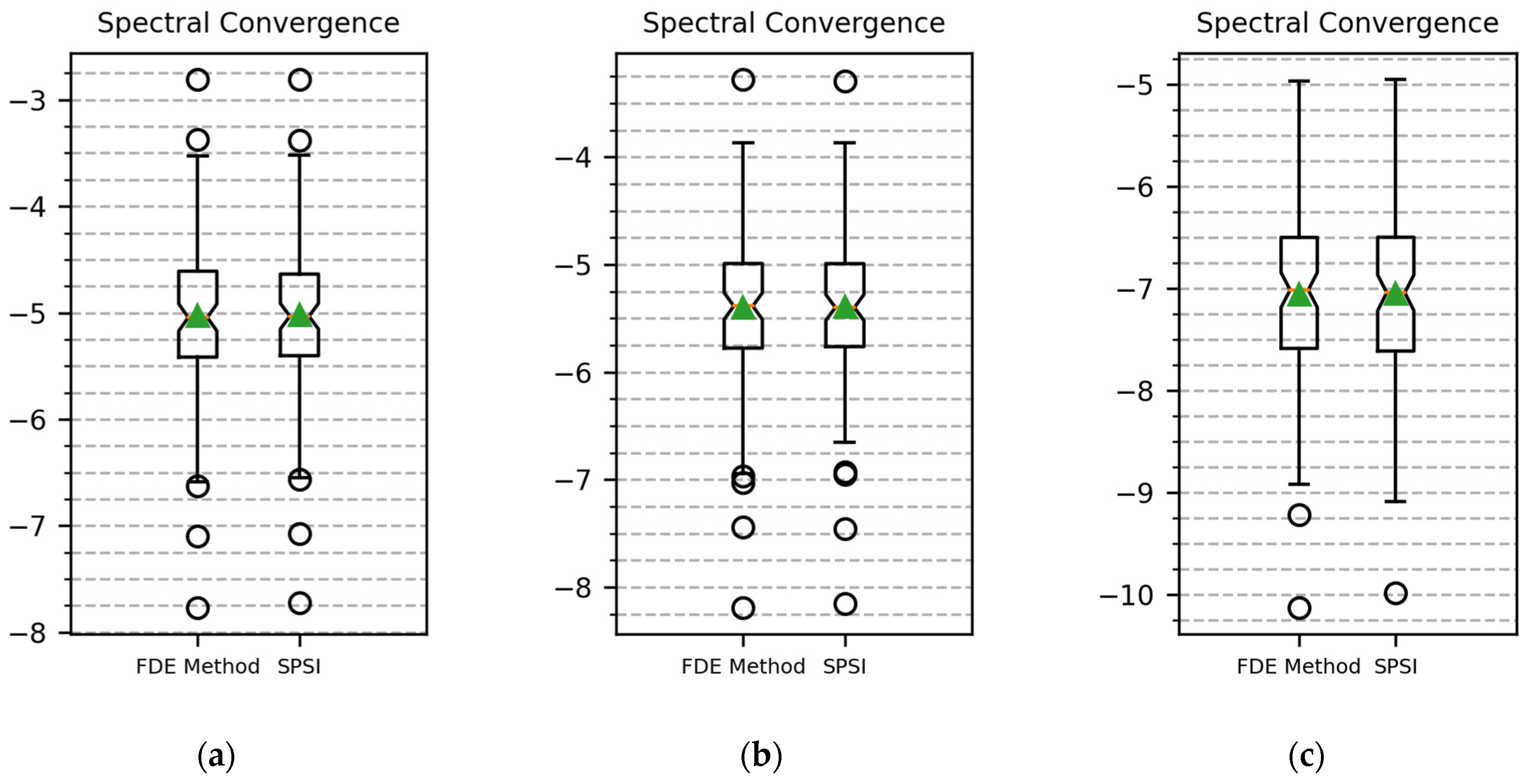
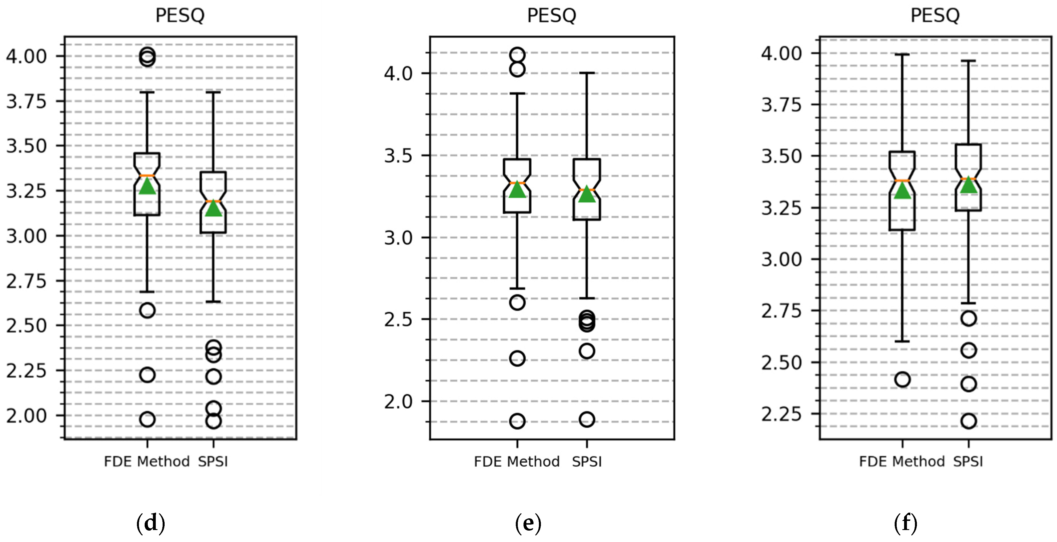
Figure 5 shows the SC and PESQ boxplots for comparison of the FDE-based method and SPSI with hop sizes of 64, 128, and 256. Table 1 gives comparisons of FDE, SPSI, and random phase concerning the average results of SC and PESQ.
Table 1 and Figure 5 show that the FDE-based method and SPSI achieved nearly identical SC results, with the FDE-based method having the slightest upper hand. In Table 1, SC performance had a greater improvement when using the FDE-based method upon increasing hop size. Due to the small differences, we can concur that the proposed FDE-based method and SPSI behaved similarly in the sense of spectrogram convergence, concerning decreasing overlap value and resolution. Inspecting the value distribution in Figure 5a–c validates this result.
In terms of the PESQ score for decreasing overlap, the FDE-based method produced better results for all different overlap values, but in the marginal case of 50% overlap. When the hop size was 64, the FDE-based method achieved a 4% increase in PESQ score concerning SPSI. From Figure 5d,e, it can be seen that the PESQ value deviation was also smaller in the cases with 87.5% and 75% overlap. It can be said that, for higher-resolution cases, which result in fewer aliases, the FDE-based method constructs perceptually better signals.
3.2. Comparison of FDE-Based Method and SPSI as Initial Values to GLA-Based Methods
The GLA repeats ISTFT and STFT iterations by considering initial phase conditions. It is based on exploiting spectrogram redundancy [1]. The convergence performance of the GLA can be further improved by introducing an additional momentum coefficient into the reconstruction. This approach is called the fast GLA (FGLA) [2]. The GLA and FGLA take into account two consistency criteria. First, for a complex-valued spectrogram X, whose amplitude is given as A, X must be a result of a Gabor transform of a set of real numbers x. Second, the amplitude of a Gabor transform of x must be equal to A. The first can be considered the hard constraint, whereas the second can be relaxed to allow applications with near 50% overlap and an auxiliary variable to increase convergence performance. Gabor transform is a special case of STFT with Gaussian windows. This method is called the GLA with an alternating direction method of multipliers (GLA-ADMM) [3].
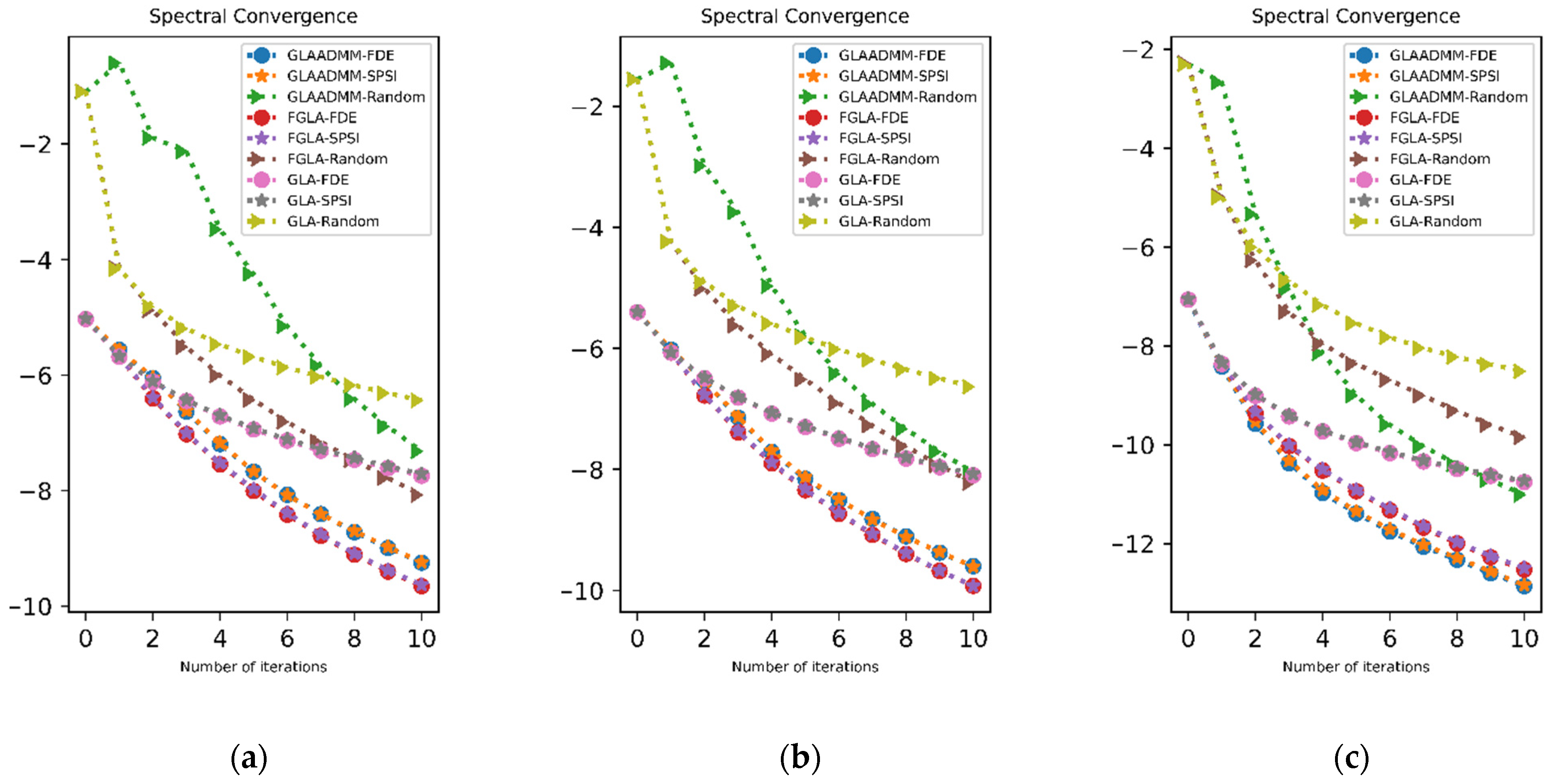
We applied the FDE-based method, SPSI, and random phase to three GLA-based iterative reconstruction methods as initial phase values and compared the deviation of SC and PESQ metrics with iterations.
In all cases, the FDE-based method produced similar, if not slightly better, results to benchmark SPSI in terms of SC. As the difference was substantially small, we can claim that the FDE-based method and SPSI would produce similar SC results for high-resolution cases when the two constraints of GLA iteration are set as hard constraints.
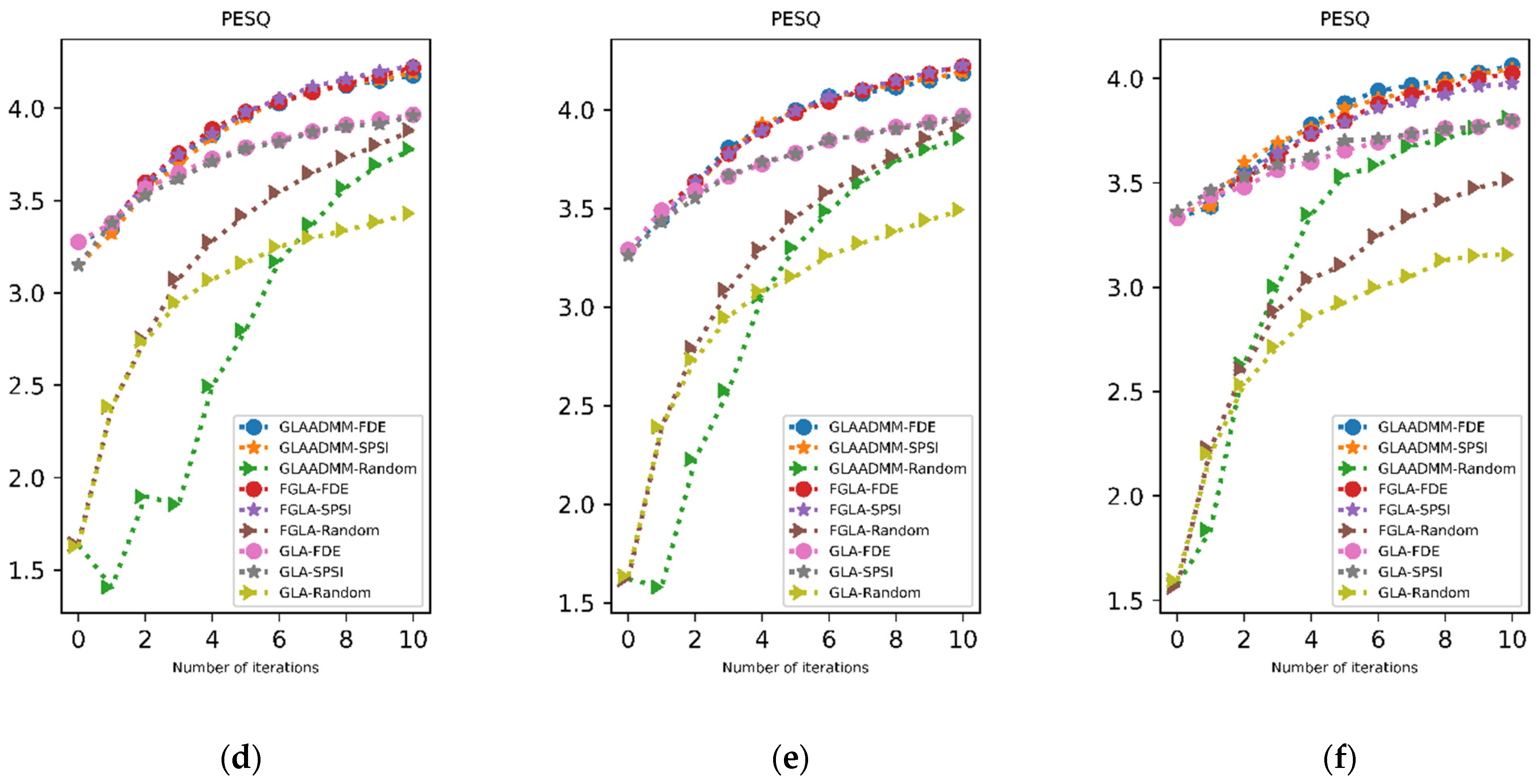
In Figure 6a,d, it can be seen that the initial results for the FDE-based method were higher than both SPSI and random phase initialization. Beginning from the first iteration, the PESQ results for FDE method-based initialization and SPSI initialization coincided. Over the iterations, all iterative methods produced similar SC and PESQ results with FDE and SPSI initialization. Figure 6b,e show similar results for increased hop size.
Upon decreasing the overlap to 50%, we can see that the GLA-ADMM method’s performance increased because it was tailored to perform better when the consistency criterion was relaxed. Figure 6c shows that, for SC evaluation, the GLA-ADMM method resulted in smaller values in the earlier part of the iteration. The small difference concerning the initialization method indicates the consistency of results with smaller hop sizes. Expectedly, the GLA-ADMM-based method also performed well in terms of the PESQ score. In Figure 6d, we can see that the evaluation curves for the FDE-based method and SPSI followed a similar trajectory with results of smaller hop sizes. Random phase initialization created a distinction for the 50% overlap case. Due to the nature of the ADMM method, the GLA-ADMM exploited random values and created a speedy increase. All in all, we can concur that the FDE-based method and SPSI can both increase GLA-based iterative reconstruction performance with similar results and produce better results than random value initialization.
4. Discussion
Although the inherent complexity of fractional-order calculus and the apparent self-sufficiency of integer order calculus has led to a relative under-exploration of applications of the fractional-order framework to signal processing, it has been shown that many systems in science and engineering can be modeled more accurately by fractional-order rather than integer-order derivatives, and many such methods have been developed to solve the problem of fractional systems. Moreover, the theory of fractals and fractional-order time-series modeling has found some applications for various sound synthesis problems. As a subtopic of sound synthesis, the audio reconstruction problem can benefit from the non-integer order differ-integration model due to its ability to model a signal memory, i.e., the dependence of a signal sample on previous samples.
We applied the fractional-order calculus framework to the audio reconstruction problem. This approach is based on conventional vocoder topologies. Unlike conventional vocoders, in this work, bandpass filter outputs around peak frequencies were modeled as fractional-order differential equations. By applying this model, we exploited the memory feature of fractionally integrated models and linked this feature to instantaneous frequency estimates. We evaluated our results using two measures. Spectral convergence is one of the most used measures for similar works, whereas PESQ is a more correlated measure with human auditory perception. We produced results using these measures concerning the window overlap. By doing so, we could evaluate method performance regarding spectrogram resolution and consistency. By applying the fractional-order framework to the phase reconstruction problem, we show that a method based on a fractional-order differential equation model can achieve better PESQ scores than the benchmark SPSI method in high-resolution conditions, along with similar spectral convergence values. Furthermore, using SPSI and the proposed FDE-based method as initialization tools for three different GLA-based methods, we show that our proposed phase reconstruction method produced similar results to benchmark SPSI on iterative algorithms.
We used FDE to model the frequency component of the phase gradient and achieved up to a 4% increase in signal reconstruction. We expect that modeling the time component of the phase gradient with FDE is also possible and that this approach can further increase evaluation performance, which will be addressed in our future research. Moreover, we can increase the adjacent point numbers for differ-integrator value estimation for the frequency component of the phase gradient and evaluate its effect on phase reconstruction performance.
Additional applications of FDE-based synthesis can be considered with neural approaches. The sinusoidal model can be suitable for voiced speech; however, unvoiced speech becomes problematic. Fractal geometry helps to model noise-like characteristics of unvoiced sounds, thereby improving the evaluation performance of modern synthesis or enhancement methods. Moreover, fractal features can be considered as neural network inputs for synthesis and enhancement applications. Additional features can increase model accuracies, especially for enhancement applications. Neural network training is notoriously time-consuming. Models that employ digital signal processing (DSP) modules as a helper for deep learning (hybrid models) have been proposed. These types of systems apply proven DSP tools to reduce the workload on neural architecture. With FDE models, two improvements are possible. Firstly, input feature size can be reduced, resulting in a decrease in the number of model parameters; secondly, signal time dependency can be modeled as a function of its relationship with long-range dependence, thereby improving the efficiency of neural models.
5. Conclusions
In this article, the fractional-order calculus framework was applied to the audio reconstruction problem. By applying this model, the memory feature of fractionally integrated models was linked to the instantaneous frequency estimate. We evaluated our results using spectral convergence and PESQ measures. We achieved up to 4% improvements in perceptually correlated PESQ measures for smaller overlaps and comparable results to the benchmark. Additionally, when using outputs from SPSI and the proposed FDE-based method, as well as random valued complex vectors, as initial values of three GLA-based methods, the proposed FDE-based phase reconstruction method produces similar results to the benchmark SPSI and substantially better results than random phase initialization on iterative algorithms.
Author Contributions
All authors contributed equally. All authors read and agreed to the published version of the manuscript.
Funding
This work was supported by the Scientific Research Projects Department of Istanbul Technical University, Project Number: MDK-2020-42479.
Data Availability Statement
Data included 50 male and 50 female speech samples from the TIMIT database, available at https://kovan.itu.edu.tr/index.php/s/wkUgteNTEtBLZ0K (accessed on 1 July 2021).
Conflicts of Interest
The authors declare no conflict of interest. The funders had no role in the design of the study; in the collection, analyses, or interpretation of data; in the writing of the manuscript; or in the decision to publish the results.
References
- Griffin, D.; Lim, J. Signal Estimation from Modified Short-Time Fourier Transform. IEEE Int. Conf. Acoust. Speech Signal Process. 1983, 8, 804–807. [Google Scholar] [CrossRef]
- Perraudin, N.; Balazs, P.; Sondergaard, P.L. A Fast Griffin-Lim Algorithm. In Proceedings of the 2013 IEEE Workshop on Applications of Signal Processing to Audio and Acoustics, New Paltz, NY, USA, 20–23 October 2013; IEEE: Piscataway, NJ, USA, 2013; pp. 1–4. [Google Scholar] [CrossRef] [Green Version]
- Masuyama, Y.; Yatabe, K.; Oikawa, Y. Griffin–Lim Like Phase Recovery via Alternating Direction Method of Multipliers. IEEE Signal Process. Lett. 2019, 26, 184–188. [Google Scholar] [CrossRef]
- Beauregard, G.T.; Harish, M.; Wyse, L. Single Pass Spectrogram Inversion. Int. Conf. Digit. Signal Process. 2015, 2015, 427–431. [Google Scholar] [CrossRef]
- Prusa, Z.; Søndergaard, P.L. Real-Time Spectrogram Inversion Using Phase Gradient Heap Integration. In Proceedings of the 19th International Conference on Digital Audio Effects (DAFx-16), Brno, Czech Republic, 5–9 September 2016; pp. 17–21. [Google Scholar]
- Prusa, Z.; Balazs, P.; Sondergaard, P.L. A Noniterative Method for Reconstruction of Phase From STFT Magnitude. IEEE/ACM Trans. Audio Speech Lang. Process. 2017, 25, 1154–1164. [Google Scholar] [CrossRef] [Green Version]
- van den Oord, A.; Dieleman, S.; Zen, H.; Simonyan, K.; Vinyals, O.; Graves, A.; Kalchbrenner, N.; Senior, A.; Kavukcuoglu, K. WaveNet: A Generative Model for Raw Audio. arXiv 2016, arXiv:1609.03499. [Google Scholar]
- Kalchbrenner, N.; Elsen, E.; Simonyan, K.; Noury, S.; Casagrande, N.; Lockhart, E.; Stimberg, F.; van den Oord, A.; Dieleman, S.; Kavukcuoglu, K. Efficient Neural Audio Synthesis. arXiv 2018, arXiv:1802.08435. [Google Scholar]
- Valin, J.M.; Skoglund, J. LPCNET: Improving Neural Speech Synthesis through Linear Prediction. In Proceedings of the 2019 IEEE International Conference on Acoustics, Speech and Signal Processing (ICASSP), Brighton, UK, 12–17 May 2019; pp. 5891–5895. [Google Scholar] [CrossRef] [Green Version]
- Masuyama, Y.; Yatabe, K.; Koizumi, Y.; Oikawa, Y.; Harada, N. Deep Griffin–Lim Iteration: Trainable Iterative Phase Reconstruction Using Neural Network. IEEE J. Sel. Top. Signal Process. 2021, 15, 37–50. [Google Scholar] [CrossRef]
- Govalkar, P.; Fischer, J.; Zalkow, F.; Dittmar, C. A Comparison of Recent Neural Vocoders for Speech Signal Reconstruction. In Proceedings of the 10th ISCA Speech Synthesis Workshop, Vienna, Austria, 20–22 September 2019; ISCA: Singapore, 2019; pp. 7–12. [Google Scholar] [CrossRef] [Green Version]
- Serra, X.; Smith, J. Spectral Modeling Synthesis: A Sound Analysis/Synthesis System Based on a Deterministic Plus Stochastic Decomposition. Comput. Music J. 1990, 14, 12. [Google Scholar] [CrossRef]
- Dolson, M. The Phase Vocoder: A Tutorial. Comput. Music J. 1986, 10, 14. [Google Scholar] [CrossRef]
- Liu, Y.-W.; Smith, J.O. Audio Watermarking through Deterministic plus Stochastic Signal Decomposition. EURASIP J. Inf. Secur. 2007, 2007, 75961. [Google Scholar] [CrossRef]
- Puckette, M. Phase-Locked Vocoder. In Proceedings of the 1995 Workshop on Applications of Signal Processing to Audio and Accoustics, New Paltz, NY, USA, 15–18 October 1995; IEEE: Piscataway, NJ, USA, 1995; pp. 222–225. [Google Scholar] [CrossRef]
- Stefanakis, N.; Abel, M.; Bergner, A. Sound Synthesis Based on Ordinary Differential Equations. Comput. Music J. 2015, 39, 46–58. [Google Scholar] [CrossRef]
- Quatieri, T.F. Discrete-Time Speech Signal Processing: Principles and Practice; Prentice Hall: Hoboken, NJ, USA, 2002. [Google Scholar]
- Das, S.; Pan, I. Fractional Order Signal Processing: Introductory Concepts and Applications; Springer: Berlin/Heidelberg, Germany, 2012. [Google Scholar] [CrossRef]
- Podlubny, I. Fractional Differential Equations: Introduction to Fractional Derivatives, Fractional Differential Equations, to Methods of Their Solution and Some of Their Applications; Academic Press: Cambridge, MA, USA, 1999. [Google Scholar]
- Petráš, I. Fractional-Order Nonlinear Systems; Nonlinear Physical Science; Springer: Berlin/Heidelberg, Germany, 2011. [Google Scholar] [CrossRef] [Green Version]
- Sabanal, S.; Nakagawa, M. The Fractal Properties of Vocal Sounds and Their Application in the Speech Recognition Model. Chaos Solitons Fractals 1996, 7, 1825–1843. [Google Scholar] [CrossRef]
- Al-Akaidi, M. Fractal Speech Processing; Cambridge University Press: Cambridge, UK, 2004. [Google Scholar]
- Lévy-Véhel, J. Fractal Approaches in Signal Processing. Fractals 1995, 03, 755–775. [Google Scholar] [CrossRef]
- Ortigueira, M.D.; Trujillo, J.J. Generalized Grünwald–Letnikov Fractional Derivative and Its Laplace and Fourier Transforms. J. Comput. Nonlinear Dyn. 2011, 6, 034501. [Google Scholar] [CrossRef]
- Assaleh, K.; Ahmad, W.M. Modeling of Speech Signals Using Fractional Calculus. In Proceedings of the 2007 9th International Symposium on Signal Processing and Its Applications, Sharjah, United Arab Emirates, 12–15 February 2007; IEEE: Piscataway, NJ, USA, 2007; pp. 1–4. [Google Scholar] [CrossRef]
- Despotovic, V.; Skovranek, T.; Peric, Z. One-Parameter Fractional Linear Prediction. Comput. Electr. Eng. 2018, 69, 158–170. [Google Scholar] [CrossRef]
- Skovranek, T.; Despotovic, V.; Peric, Z. Optimal Fractional Linear Prediction With Restricted Memory. IEEE Signal Process. Lett. 2019, 26, 760–764. [Google Scholar] [CrossRef]
- Skovranek, T.; Despotovic, V. Audio Signal Processing Using Fractional Linear Prediction. Mathematics 2019, 7, 580. [Google Scholar] [CrossRef] [Green Version]
- Maragos, P.; Young, K.L. Fractal Excitation Signals for CELP Speech Coders. In Proceedings of the International Conference on Acoustics, Speech, and Signal Processing, Albuquerque, NM, USA, 3–6 April 1990; IEEE: Piscataway, NJ, USA, 1990; pp. 669–672. [Google Scholar] [CrossRef]
- Maragos, P.; Potamianos, A. Fractal Dimensions of Speech Sounds: Computation and Application to Automatic Speech Recognition. J. Acoust. Soc. Am. 1999, 105, 1925–1932. [Google Scholar] [CrossRef] [PubMed]
- Tamulevičius, G.; Karbauskaitė, R.; Dzemyda, G. Speech Emotion Classification Using Fractal Dimension-Based Features. Nonlinear Anal. Model. Control 2019, 24. [Google Scholar] [CrossRef]
- Pitsikalis, V.; Maragos, P. Analysis and Classification of Speech Signals by Generalized Fractal Dimension Features. Speech Commun. 2009, 51, 1206–1223. [Google Scholar] [CrossRef] [Green Version]
- Tarasov, V.E.; Tarasova, V.V. Long and Short Memory in Economics: Fractional-Order Difference and Differentiation. IRA-Int. J. Manag. Soc. Sci. 2016, 5, 327. [Google Scholar] [CrossRef] [Green Version]
- Geweke, J.; Porter-Hudak, S. The Estimation and Application of Long Memory Time Series Models. J. Time Ser. Anal. 1983, 4, 221–238. [Google Scholar] [CrossRef]
- Garofolo, J.S.; Lamel, L.F.; Fisher, W.M.; Fiscus, J.G.; Pallett, D.S. DARPA TIMIT Acoustic-Phonetic Continuous Speech Corpus CD-ROM. NIST Speech Disc. 1-1.1 [CD-ROM]; US Department of Commerce: Washington, DC, USA, 1993.
- Loizou, P.C. Speech Enhancement: Theory and Practice, 2nd ed.; CRC Press: Boca Raton, FL, USA, 2017. [Google Scholar]
- Le Roux, J.; Kameoka, H.; Ono, N.; Sagayama, S. Fast Signal Reconstruction From Magnitude STFT Spectogram Based on Spectogram Consistency. In Proceedings of the 13th International Conference on Digital Audio Effects (DAFx-10), Graz, Austria, 6–10 September 2010; pp. 1–7. [Google Scholar]
Figure 1.
Proposed instantaneous frequency estimation with fractional differential equation models around spectrogram peak frequencies.
Figure 1.
Proposed instantaneous frequency estimation with fractional differential equation models around spectrogram peak frequencies.

Figure 2.
Regression lines around a peak with respect to beta: (a) case a: 0; (b) case b: 0.

Figure 3.
Calculating estimated instantaneous frequency: (a) when = 0, the normal to the regression line points to the peak frequency bin; (b) upon changing slope of the regression line, the intersection point of the normal line on the frequency axis moves away.
Figure 3.
Calculating estimated instantaneous frequency: (a) when = 0, the normal to the regression line points to the peak frequency bin; (b) upon changing slope of the regression line, the intersection point of the normal line on the frequency axis moves away.

Figure 4.
Proposed signal reconstruction flow.

Figure 5.
SC and PESQ boxplots for different hop sizes: (a) SC boxplot of FDE method and SPSI for hop size = 64, overlap = 87.5%; (b) SC boxplot of FDE method and SPSI for hop size = 128, overlap = 75%; (c) SC boxplot of FDE method and SPSI for hop size = 256, overlap = 50%; (d) PESQ boxplot of FDE method and SPSI for hop size = 64, overlap = 87.5%; (e) PESQ boxplot of FDE method and SPSI for hop size = 128, overlap = 75%; (f) PESQ boxplot of FDE method and SPSI for hop size = 256, overlap = 50%.


Figure 6.
GLA, FGLA, and GLAADMM comparison with SPSI, FDE method, and random phase values as initial phases: (a) SC for 10 iterations for hop size = 64, overlap = 87.5%; (b) SC for 10 iterations for hop size = 128, overlap = 75%; (c) SC for 10 iterations for hop size = 256, overlap = 50%; (d) PESQ for 10 iterations for hop size = 64, overlap = 87.5%; (e) PESQ for 10 iterations for hop size = 128, overlap = 75%; (f) PESQ for 10 iterations for hop size = 256, overlap = 50%.


Table 1.
Mean SC and PESQ measurement results of SPSI, FDE method, and random phase concerning increasing hop size.
Table 1.
Mean SC and PESQ measurement results of SPSI, FDE method, and random phase concerning increasing hop size.
| Hop Size | Method | SC | PESQ |
|---|---|---|---|
| 64 (87.5% overlap) | SPSI | −5.02086 | 3.150896 |
| FDE Method | −5.02798 | 3.27584 | |
| Random | −1.08779 | 1.644972 | |
| 128 (75% overlap) | SPSI | −5.39316 | 3.261765 |
| FDE Method | −5.39769 | 3.289174 | |
| Random | −1.55655 | 1.627104 | |
| 256 (50% overlap) | SPSI | −7.05101 | 3.360622 |
| FDE Method | −7.06164 | 3.331025 | |
| Random | −2.30093 | 1.579338 |
Publisher’s Note: MDPI stays neutral with regard to jurisdictional claims in published maps and institutional affiliations. |
© 2021 by the authors. Licensee MDPI, Basel, Switzerland. This article is an open access article distributed under the terms and conditions of the Creative Commons Attribution (CC BY) license (https://creativecommons.org/licenses/by/4.0/).
Share and Cite
MDPI and ACS Style
Yazgaç, B.G.; Kırcı, M. Fractional Differential Equation-Based Instantaneous Frequency Estimation for Signal Reconstruction. Fractal Fract. 2021, 5, 83. https://doi.org/10.3390/fractalfract5030083
AMA Style
Yazgaç BG, Kırcı M. Fractional Differential Equation-Based Instantaneous Frequency Estimation for Signal Reconstruction. Fractal and Fractional. 2021; 5(3):83. https://doi.org/10.3390/fractalfract5030083
Chicago/Turabian StyleYazgaç, Bilgi Görkem, and Mürvet Kırcı. 2021. "Fractional Differential Equation-Based Instantaneous Frequency Estimation for Signal Reconstruction" Fractal and Fractional 5, no. 3: 83. https://doi.org/10.3390/fractalfract5030083