
Surface Roughness in RANS Applied to Aircraft Ice Accretion Simulation: A Review


1
Mechanical Engineering Department, École de Technologie Supérieure, Montréal, QC H3C 1K3, Canada
2
University Bordeaux, INRIA, CNRS, Bordeaux INP, IMB, UMR 5251, 33405 Talence, France
*
Author to whom correspondence should be addressed.
Fluids 2023, 8(10), 278; https://doi.org/10.3390/fluids8100278
Submission received: 29 August 2023
/
Revised: 7 October 2023
/
Accepted: 10 October 2023
/
Published: 15 October 2023
(This article belongs to the Collection Challenges and Advances in Heat and Mass Transfer)
Abstract
:Experimental and numerical fluid dynamics studies highlight a change of flow structure in the presence of surface roughness. The changes involve both wall heat transfer and skin friction, and are mainly restricted to the inner region of the boundary layer. Aircraft in-flight icing is a typical application where rough surfaces play an important role in the airflow structure and the subsequent ice growth. The objective of this work is to investigate how surface roughness is tackled in RANS with wall resolved boundary layers for aeronautics applications, with a focus on ice-induced roughness. The literature review shows that semi-empirical correlations were calibrated on experimental data to model flow changes in the presence of roughness. The correlations for RANS do not explicitly resolve the individual roughness. They principally involve turbulence model modifications to account for changes in the velocity and temperature profiles in the near-wall region. The equivalent sand grain roughness (ESGR) approach emerges as a popular metric to characterize roughness and is employed as a length scale for the RANS model. For in-flight icing, correlations were developed, accounting for both surface geometry and atmospheric conditions. Despite these research efforts, uncertainties are present in some specific conditions, where space and time roughness variations make the simulations difficult to calibrate. Research that addresses this gap could help improve ice accretion predictions.
1. Introduction
Fluid dynamics studies, both experimental and numerical, intend to understand the fluid flow inside or above complex geometries. Among the applications often encountered are flows in pipes [1], flows around aerial or terrestrial vehicles [2,3] or flows and wind in urban zones [4]. On the computational fluid dynamics (CFD) side, the simplest approach to model the walls and solid parts of the geometry is to assume smooth surfaces [5,6]. The smooth approach has its limits. In practice, several geometries have irregular surfaces with roughness of various origins. Wear, deposit, for example in turbines [7], and ice accretion on an aircraft surface [8] cause roughness. Experimental studies showed different flow structures and behaviour between rough and smooth surfaces [9]. The influence of roughness is mainly concentrated in the near-wall region and affects the turbulent boundary layer [10], particularly the inner layer. The boundary layer modification increases flow metrics such as the wall heat transfer and the skin friction [11]. Experimental studies have tackled this for decades [12,13], highlighting heat transfers, and skin friction increases in the presence of roughness. Therefore, the mathematical models used in CFD should account for roughness to produce accurate predictions.
CFD simulations can either resolve the flow around individual roughness elements or model the effects of roughness. Direct Numerical Simulation (DNS) is one possible way to resolve a flow around surface roughness elements. DNS became popular over the last decade, with the increase in computational power [14,15]. Large Eddy Simulation (LES) also resolves individual roughness elements, but with a lower computational cost [16,17]. Nevertheless, the computational cost of DNS and LES limits their application to simple geometries and is impractical for industrial problems. The modeled approaches present better applicability and wider ranges of use compared to the resolved approaches. The Reynolds Averaged Navier–Stokes (RANS) is popular in an industrial context since it does not require as much computational power as DNS or LES [18].
The RANS models the effects of turbulent fluctuations with an additional stress term in the Navier–Stokes equations. This stress term is usually assumed proportional to the wall normal velocity gradient, and the proportionality factor is called the eddy viscosity. The eddy viscosity turbulence models, such as the Spalart–Allmaras (SA) model [19] or the k-ω model [20], compute the eddy viscosity by solving one (SA) or two (k-ω) transport equations. In a context of rough geometries with RANS, these turbulence models are commonly adapted to account for roughness [21,22]. Experimental skin friction obtained using manufactured roughness patterns help calibrate the rough turbulence models [12]. Sometimes, the rough turbulence models over predict the wall heat fluxes [23]. This inaccuracy led to the development of so-called thermal correction models aiming to reduce the heat fluxes. Morency and Beaugendre [23], Chedevergne [24], Suga et al. [11], and Aupoix [25] derived thermal corrections to use with the rough turbulence models. Most of the thermal correction models increase the turbulent Prandtl number to reduce the wall heat fluxes. The correction depends on the roughness geometric characteristics. Apart from the rough turbulence models, the discrete element roughness method (DERM) is another modeled approach used in CFD [26,27]. The DERM directly adds the roughness effects in the mass, momentum, and energy equations of the flow. The DERM adds source terms to the flow equations to account for blockage, drag, and heat transfer induced by roughness [28]. Chedevergne recently used the DERM helped by experimental surface topography measurements to finely quantify the source terms in the model [29]. The intensity of the additional source terms varies with the roughness geometric characteristics.
Experimental setups can characterize the roughness geometries. Modern measurement techniques allow a precise mapping of experimental surfaces, for example with laser measurements [30]. Particle velocimetry methods are able to measure the velocity around rough surfaces [31], helping in the identification of typical flow structures. Roughness measurements show highly irregular roughness patterns in most engineering applications [32]. These irregular patterns are usually non-trivial to input in the CFD models, since uncertainty persists. A roughness pattern requires quantifiable metrics to model it with CFD. Common metrics statistically characterize the height and/or spacing of the roughness elements on a surface [33], and are used to describe a given roughness pattern. For RANS turbulent flow description, one popular metric is the equivalent sand grain roughness (ESGR) height, ks, introduced almost one century ago by Nikuradse [34]. The ESGR height allows the definition of a roughness pattern with a single metric. ks is the diameter of the packed spheres that would give the same skin friction as the actual real roughness pattern [12], obtained experimentally or geometrically resolved with DNS. ks is relevant for random and regular roughness patterns similar to sand grain paper. For regular roughness patterns, correlations related ks to some geometrical parameters of the roughness elements [35,36]. However, this single metric can fail to predict the skin friction for highly irregular roughness patterns, for example, in a context of ice-induced roughness on an aircraft [37].
Aircraft icing is a specific application of flow over a rough surface. At the early stages, ice accretion creates surface roughness that increases the wall heat transfer and modifies the final ice shape [38]. For CFD-based ice accretion simulations, the usual framework employs a RANS airflow solver, a droplet impingement solver, and an accretion solver [39]. The RANS airflow solver must model surface roughness to increase the wall heat transfer and the wall skin friction [8]. ks is used to characterize the roughness pattern in most ice accretion software, for example in FENSAP-ICE [40], IGLOO3D [41], or LEWICE [42]. Ice-specific semi-empirical correlations are developed to relate the roughness pattern to the atmospheric conditions and the airfoil geometry [43,44,45,46]. In most ice accretion software, the surface roughness imposed in the model is constant and uniform all over the surface [47], even if experimental observations show non-uniform roughness patterns over the airfoil surface [43,48,49]. A recent study followed these observations and derive non-uniform roughness distributions [50] to obtain a heat transfer distribution closer to the experiment. Research efforts are still needed to improve the roughness models as some ice accretion simulations fail at predicting a satisfactory ice shape compared to the experiment [51].
This review paper investigates both RANS approaches with wall resolved boundary layers (denoted as wall resolved RANS for the rest of the paper) that account for roughness in aeronautics flows and the special case of ice-induced roughness in aircraft in-flight icing. The objective is to review (1) how roughness is modeled in RANS in the scope of the ESGR and (2) what the specific roughness treatments required for aircraft icing are. First, the roughness geometrical characterization is depicted, with a focus on the usual metrics and the ESGR approach. Second, the roughness impact on the turbulent flow structures is depicted, highlighting some rough turbulence model implementations for wall resolved RANS. Finally, the roughness impact on the in-flight aircraft ice accretion is detailed. This last section also highlights the semi-empirical correlations and models for ice-induced roughness description.
2. Roughness Geometrical Characterization in Aerodynamics
This section gives an insight on how the presence of roughness impacts the flow structure in the boundary layer. The first subsection develops the roughness pattern characterizations classically employed in CFD, such as the statistical metrics. The second subsection focuses on the particular case of the ESGR height, a metric typically used in RANS applications.
2.1. Geometrical Parameters
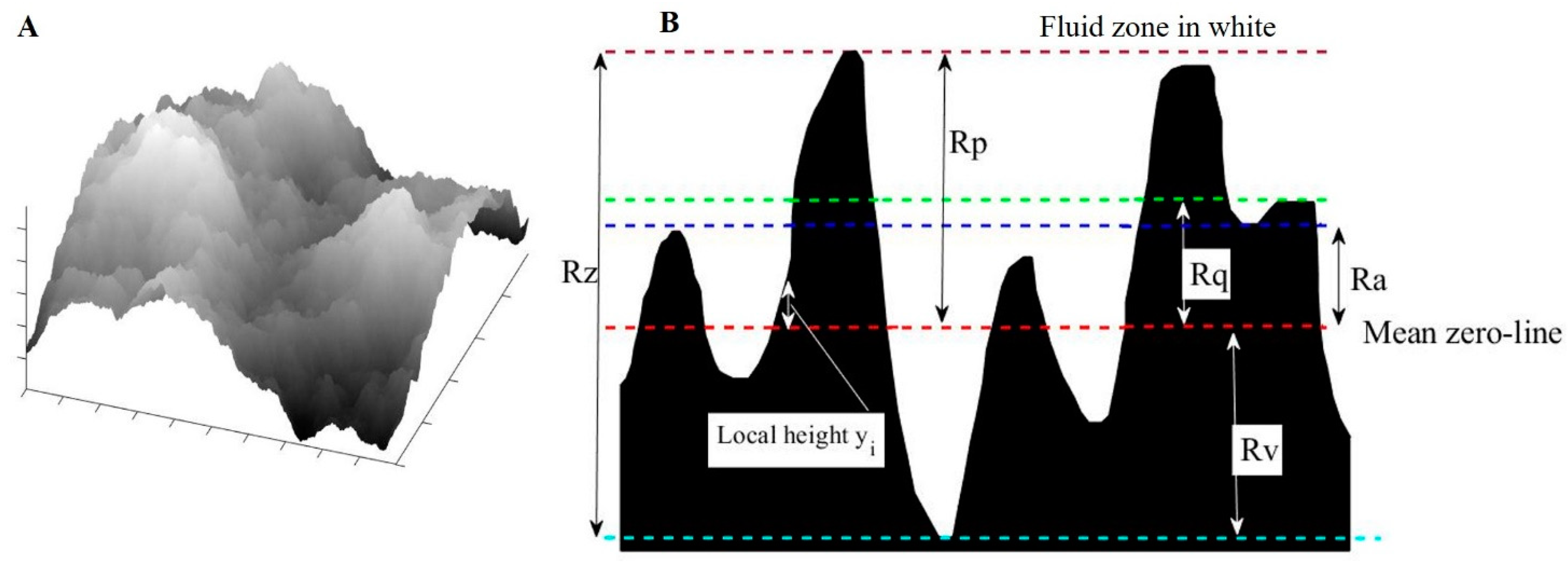
In engineering, the spectrum of roughness patterns encountered varies from regular well-ordered configurations to highly irregular and uncertain geometries such as in ice accretion [52] or heterogeneous surface state [53]. Roughness patterns are mathematically described by quantifiable parameters. Through the years, standards have normalized the description of surface states. The SAE J448 [54], the ISO 1302 norm [33,55,56], or the ISO 4287 norm [57] are among the international standards used. The parameters are defined either on a slice of the surface to represent the peaks and valleys amplitudes, or on an area to finely represent the spatial organization of the surface. The main metrics encountered for a surface description are:
- Ra, the arithmetic mean height;
- Rq, the root mean square height;
- Rv, the maximum valley depth;
- Rp, the maximum peak height;
- Rz, the maximum peak to valley height;
- Sk, the skewness;
- Ku, the kurtosis.
Figure 1 represents a generic rough area and a slice of a rough surface and identifies the most common amplitude metrics. For a rough profile sampled with n points, each one with a height yi from the smooth mean-zero line, the expressions for the previous parameters are given in Equations (1)–(7).
In the cases of 3D roughness patterns covering an area, some authors introduced spatial parameters to account for the spacing and the wetted and/or frontal area of the roughness [58]. The shape parameter Λ is a roughness parameter commonly used in the literature. The shape parameter suggested by Dirling [35] is a function of the average roughness element spacing d, the roughness height k, the frontal area of a roughness element Af, and the total windward wetted area of a roughness element As. Equation (8) presents the mathematical definition of the shape parameter defined by Dirling.
Sigal and Danberg [36] introduced a modified definition of the shape parameter by using a surface ratio to account for the roughness element proximity. The total smooth surface S, before roughness addition, and the total frontal area Sf are accounted for in the expression (Equation (9)). The value of the exponent suggested by Sigal and Danberg was calibrated to match Schlichting’s data [59].
The correlations of Dirling and Sigal and Danberg require the geometric characteristics of a single roughness element, such as Af or As. These correlations are based on regular roughness elements such as spheres, cones, or rods. Therefore, the correlations may not be sufficient for irregular roughness with various geometries. To include such irregular cases, van Rij et al. [60] suggested another variant of the shape parameter definition. The total roughness windward wetted area Ss is used in that case (Equation (10)). This definition requires detailed representations of the roughness pattern to extract Ss.
These geometrical features are useful to calculate an important parameter for the rough turbulent flow: the equivalent sand grain roughness.
2.2. The Equivalent Sand Grain Roughness (ESGR)
To quantify the roughness effects, the ESGR constitutes a length scale often used in engineering fields. Nikuradse [34] carried out experiments with sand-grain-like roughness patterns. The roughness pattern was modeled as packed identical spheres whose diameter is called the sand grain roughness (SGR) height. This approach suits regular roughness patterns with a sand-grain texture well. For irregular roughness, Colebrook et al. [61] introduced the ESGR height, often denoted ks. The ESGR height relates non-uniform roughness patterns effects to the SGR height effects on the boundary layer [58]. The mathematical definition of the ESGR is obtained knowing the flow velocity U at a normal distance y above the surface [59]. denotes the friction velocity and κ is the von Kármán constant.
Without the knowledge of U(y), the ESGR height is correlated to the geometrical configuration of the roughness elements. Dirling [35] established a correlation for cones or spheres elements. Bons [7,62] worked on correlations for turbine blades roughness. Sigal and Danberg [36] derived ESGR correlations for transversal roughness such as bars and rods, while van Rij et al. [60] developed correlations for 3D irregular roughness. Botros [13] recently extended the pioneer studies of Nikuradse and Colebrook for steel pipes. Table 1 presents some correlations used to compute the ESGR ks.
3. Roughness Regimes and Rough Turbulence Models
This section depicts roughness impacts on the flow structure and reviews how RANS models tackle roughness. The first subsection shows how the presence of roughness in a flow alters the boundary layer, defining the roughness regimes encountered. The second subsection presents some RANS approaches used to include the roughness in the computation, including the velocity and thermal corrections required to model the flow over a rough surface.
3.1. The Rough Flow Regimes
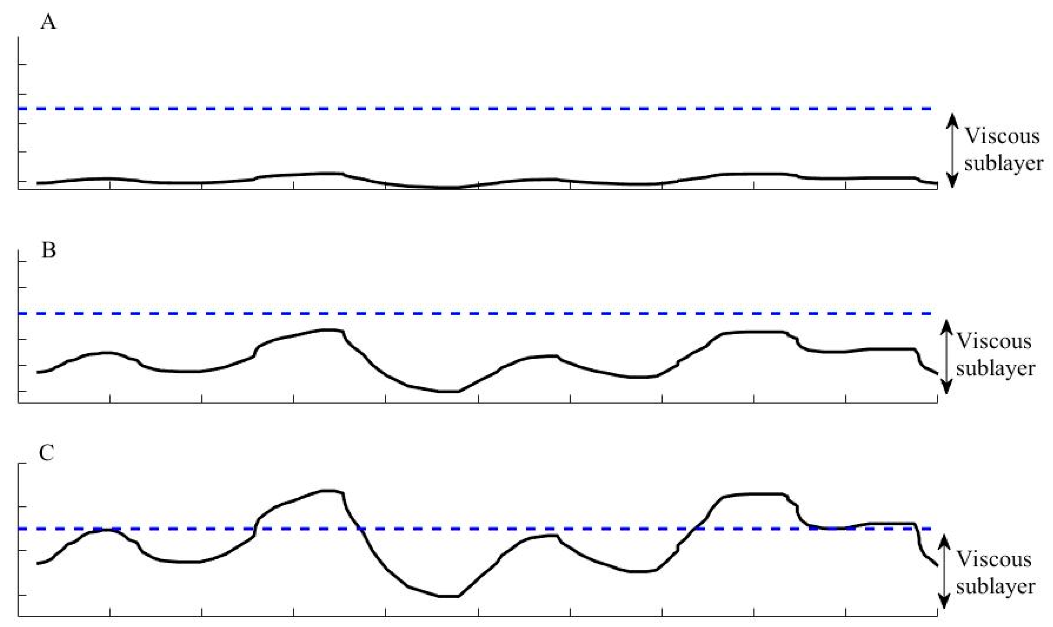
The roughness modifies the near-wall flow behavior compared to a smooth surface. Smooth surfaces were extensively studied for almost a century with the definition of the so-called law-of-the-wall [63,64,65]. The smooth theory was extended to rough surfaces to face industrial applications. For the rough turbulent boundary layer, a roughness Reynolds number is defined. The symbol ν appearing in Equation (12) stands for the kinematic viscosity of air.
Three main roughness regimes can be observed:
- The hydraulically smooth regime if
- The transitionally rough regime if
- The fully rough regime if
Qualitatively, these regimes, illustrated in Figure 2, correspond to:
- Roughness elements small compared to the viscous sublayer thickness (hydraulically smooth);
- Roughness elements in the same order of thickness as the viscous sublayer thickness (transitionally rough); and
and delimit the regimes and take different values depending on the type of roughness encountered. Nikuradse [34] was a pioneer in the field and suggested values for uniform sand grain roughness. Ligrani and Moffat [67] suggested values for spherical roughness elements. Langelandsvik et al. derived tailored values for commercial steel piping [68]. Schultz and Flack [69] established values for surface scratches. These common values are:
- Nikuradse: and
- Ligrani and Moffat: and
- Langelandsvik et al.: and
- Schultz and Flack: and
These theoretical and experimental developments are the basis for the CFD models aiming at accounting for surface roughness. The most common implementations used for RANS modeled approaches are reviewed in the following subsection.
3.2. RANS Implementations to Account for Roughness
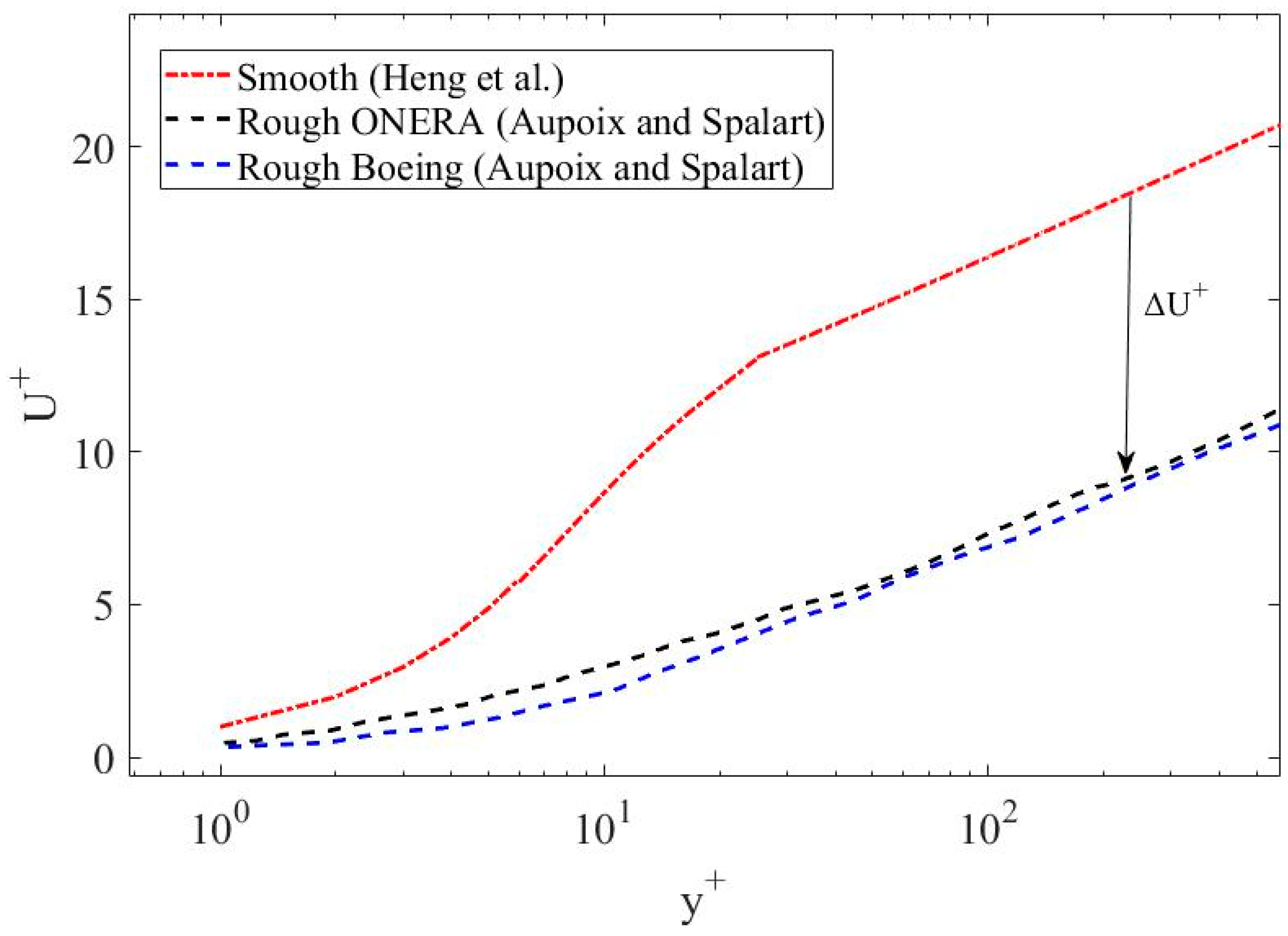
The roughness effects mainly create a velocity deficit in the boundary layer compared to a smooth surface. This leads to a downward shift of the log-Law by a value ΔU+ [58], as in Equation (13) where C is a constant.
This theoretical shift is confirmed by experimental studies for example from ONERA and Boeing [21], compared to the smooth profile [65], as illustrated in Figure 3.
The velocity shift indicates an increase in the friction velocity, and by extension, in the wall shear stress and skin friction coefficient. The amplitude of the velocity shift is a function of the roughness parameters, mainly . Therefore, RANS requires to accurately model the velocity shift ΔU+ to accurately predict the rough skin friction.
To account for roughness in a RANS model, the turbulence models are adapted. A decade after its original publication, the Spalart–Allmaras (SA) turbulence model [19] received a rough extension [21]. The original SA turbulence model solves one transport equation for the turbulence variable . The computation of the turbulent variable enables the knowledge of the turbulent eddy viscosity μt, function of the wall distance, required for the RANS equations closure. The rough version of the SA turbulence model redefines the wall distance from its smooth value d to drough, using the ESGR.
The main modification of the SA turbulence model is the wall boundary condition, which is for a smooth case. For the rough version, a gradient normal to the wall, with n being the normal direction, is imposed.
Similarly, the two-equation k-ω turbulence model [20], gained its roughness extensions through the years. Wilcox [70] was the first to derive a rough extension in 1998 before adding some corrections in 2006. The wall boundary condition for the parameter ω is altered. ρ is the fluid density and μ is the dynamic viscosity.
With
This model has the disadvantage of requiring a very fine mesh in the near wall [71] and is not fully compatible with the original SST formulation [72]. Later, Knopp et al. [73] suggested a new formulation for the rough k-ω turbulence model to improve the weaknesses of the original rough extension. Apart from the SA and k-ω turbulence models, the k-ε model also received its rough extension [74]. These rough versions predict accurate skin frictions compared to experimental data [23]. This allows an evaluation of the friction velocity and of the roughness Reynolds number (Equation (12)).
Several studies showed that the rough velocity profile and the velocity shift ΔU+ (see Figure 3) are functions of the roughness Reynolds number [75,76,77]. Equation (18) shows Nikuradse [34] estimation for the rough log-Law in a fully rough regime.
More recently, Radenac et al. [77] suggest using the relation developed by Grigson [76] based on the work of Colebrook [61] to directly estimate the velocity shift.
Another alternative, developed by Kays and Crawford [75], gives a variant to compute the velocity shift.
Although most correlations are valid in a fully rough regime, others are derived to fit all regimes. Following the works from Nikuradse, Equation (21) covers all regimes from hydraulically smooth Equation (21a) to transitionally rough Equation (21b) and fully rough (Equation (21c)) [10].
In all models, the velocity shift is zero in a hydraulically smooth regime. For very small roughness elements, the effects on the flow vanish due to the viscosity [10,78]. Commercial CFD software with wall resolved RANS approaches, such as STAR-CCM+, implement the roughness effect such as Equation (21) [79]. By default, the constants 5.23 and 0.253 in Equation (21) are set but tunable by the user, such as the values for and .
Even if the skin friction is accurate, the wall heat transfer is not correctly predicted for some rough cases. Past studies [11,23,25] reported an overestimation of the wall heat fluxes when the rough turbulence models are employed. Similar to the velocity profile, the temperature profile is shifted in the boundary layer [25] above roughness. Kays and Crawford [75] gave a formulation for the temperature shift ΔT+, where Prt is the turbulent Prandtl number and CPr is a function of the laminar Prandtl number Pr.
The prediction of the wall heat transfer in the RANS models requires to accurately predict the temperature shift ΔT+.
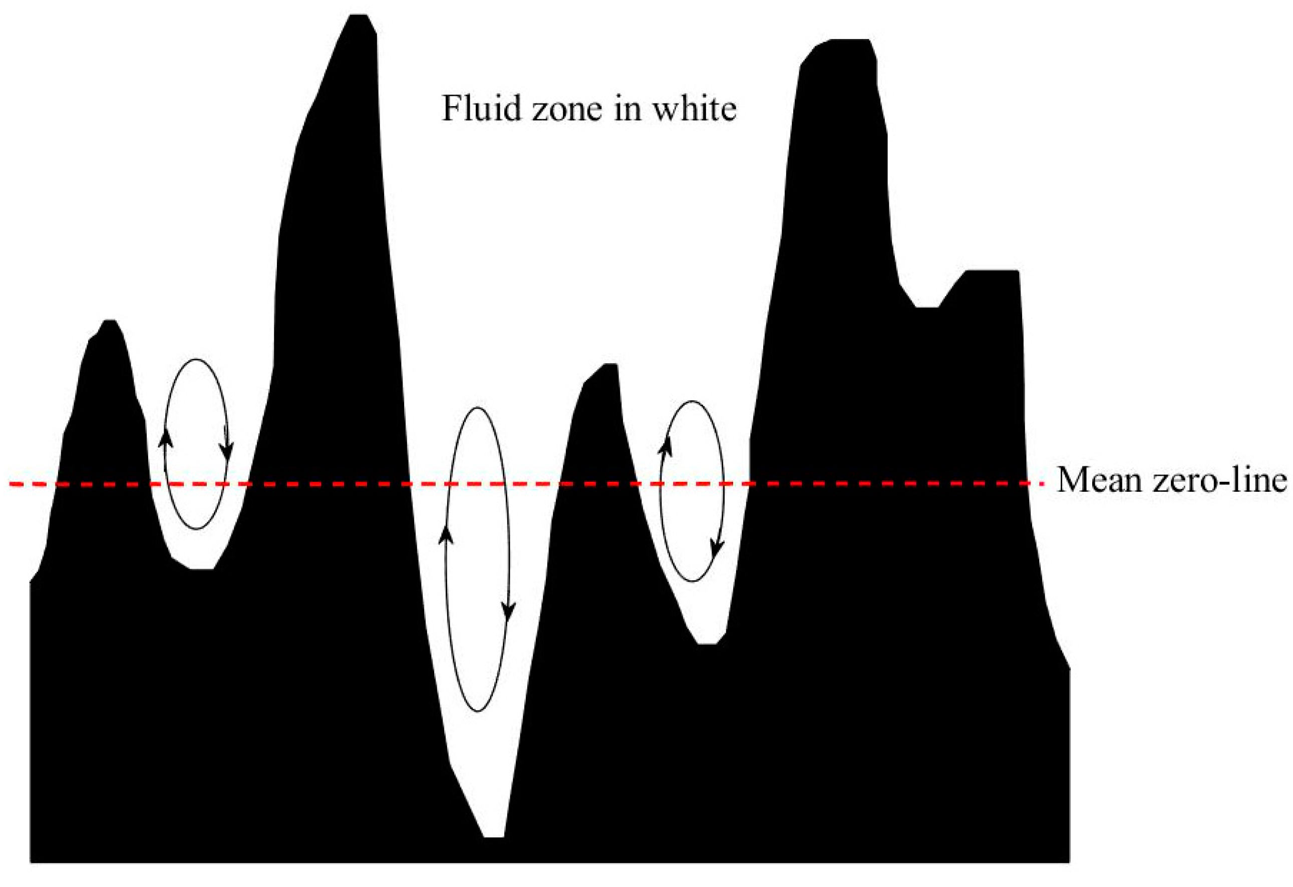
According to the investigations of Suga et al. [11], the heat flux overestimation comes from the trapped recirculating flow between the roughness elements. These recirculation zones create a thermal barrier reducing the heat flux, as schemed in Figure 4.
The thermal correction models [11,23,25] intend to account for these recirculation zones. The common approach in the literature is to locally increase the turbulent Prandtl number Prt. This impacts both the thermal conductivity and the temperature shift (Equation (22)). The thermal correction models add ΔPrt to the turbulent Prandtl number, allowing the modification of the thermal conductivity.
Suga et al. [11] derived the following expression for the turbulent Prandtl number correction, where εs and εy are the local turbulent kinetic energy at the ESGR height and at the height y from the wall, respectively.
The thermal correction model from Suga et al. only requires one roughness parameter, ks, to compute the thermal correction.
Morency and Beaugendre [23] derived a 2-parameter thermal correction model by blending the works from Ligrani et al. [80], Dipprey and Sabersky [81], and Owen and Thomson [82], and the integral method from Kays and Crawford [75]. The general form of is inspired from the thermal correction model from Aupoix [25].
The expression of F is given by Equation (27).
The factor g damps the correction in a transitionally rough regime. The limits used to separate the hydraulically smooth ), transitional, and fully rough ( regimes corresponds to the and values suggested by Nikuradse [34].
A third thermal correction model is the 3-parameter model of Aupoix [25]. The turbulent Prandtl number correction is the same as in Equation (26), but with an alternate definition for the factor F, function of the velocity shift ΔU+, and a geometrical correction parameter Scorr. Scorr corresponds to the ratio between the rough wetted area (i.e., accounting for the wetted area of the roughness elements) and the smooth wetted area, with the through below the recirculation zone (see Figure 4) neglected. The factor F is expanded in Equation (28).
The factors A and B are defined in the following Equations (29) and (30).
ΔU+ being a function of , the correction suggested by Aupoix requires three roughness parameters: ks; k; and Scorr.
The RANS models depicted in this subsection predict both wall shear stress and wall heat flux over roughness. The next section gives an insight into a specific application of rough surfaces: aircraft icing.
4. The Specific Case of Aircraft Icing
In-flight ice accretion simulation commonly relies on RANS and rough turbulence to model airflow. This section first depicts the models used in aircraft ice accretion simulations and how surface roughness plays a key role in the process. The second subsection reviews the roughness semi-empirical correlations developed to determine the roughness pattern above ice surfaces.
The Ice Accretion Process: A Roughness-Dependent Phenomenon
Ice accretion studies address the safety concerns induced by ice build-up on aircraft surfaces [83,84]. The studies apply to both ice-induced aerodynamic degradation [85,86] and shedding debris [87,88]. Initially carried out experimentally [38,45,89], ice accretion studies have been supplemented by numerical simulations with the increase of computational power [52,90,91].
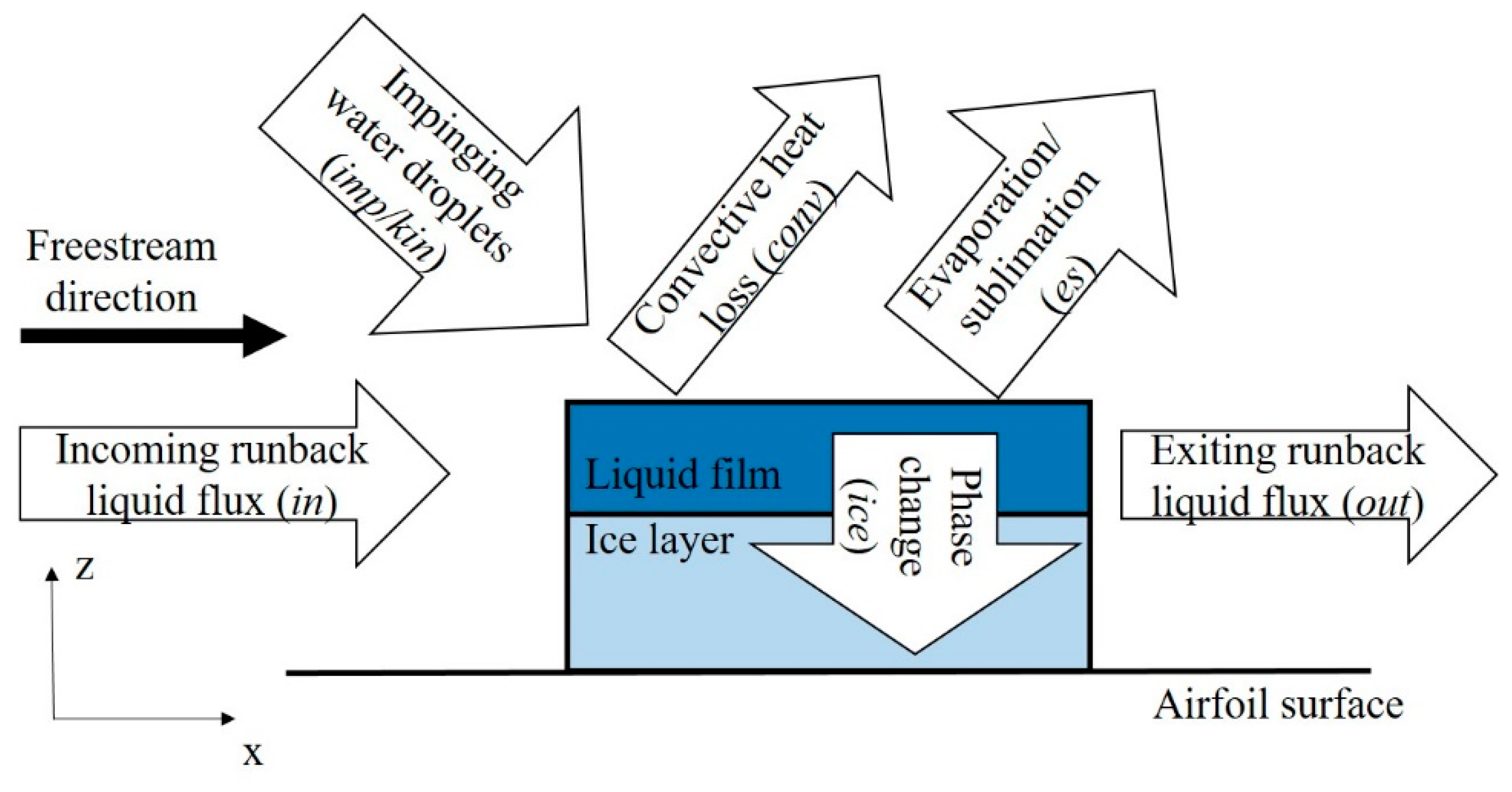
For numerical simulations, Messinger [92] pioneer works develop a well-known model to compute the ice growth on an aircraft surface. The Messinger model has been improved through the years to include features such as unsteadiness, shear-stress driven liquid film, or partial differential equation formulation [93,94,95,96]. The original Messinger model computes the mass and the energy balance in a control volume composed of a moving liquid film and an ice layer, as shown in Figure 5.
The white arrows in Figure 5 symbolize the main contributions to the mass balance (Equation (31)) and the energy balance (Equation (32)) where (kg/s) and (J/s) are the mass flux rate and energy flux rate, respectively. The subscripts correspond to the ones illustrated in Figure 5.
The accretion can be seen as a phase change problem where the liquid film freezes, releasing latent heat during the process. In a control volume, the water phase is determined by the internal energy. If the energy in the control volume is lower than the solidification energy, the water is solid. If the energy in the control volume is higher than the fusion energy (the solidification energy plus the latent heat of phase change), the water is liquid. When the total energy of the control volume is between the energy of solidification and the energy of fusion, ice and liquid water coexist, and a glaze ice state is observed. The contributions remain almost identical among the ice accretion models, with some additions such as the radiation or the conductivity through ice [47,97]. The variables in Equations (31) and (32) were described by Özgen and Canibek [98]. Among the variables, several depend on quantities obtained at the airflow computation step, such as the heat transfer coefficient htc obtained from the wall heat flux ϕ, the wall temperature T, and the recovery temperature Trec.
More precisely:
- The evaporation/sublimation mass and energy variables depend on the heat transfer coefficient [99];
- The convective heat loss is a function of the heat transfer coefficient;
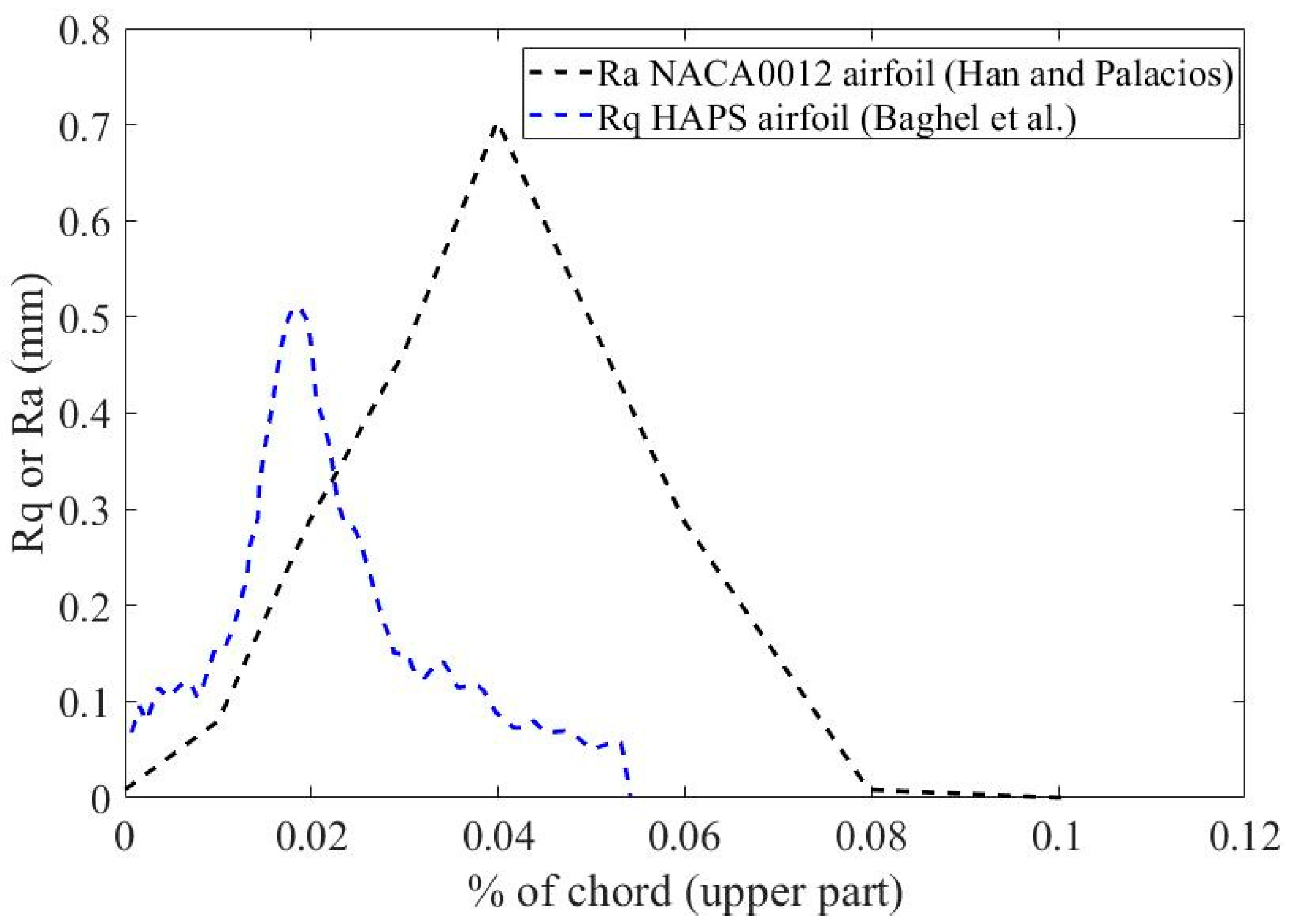
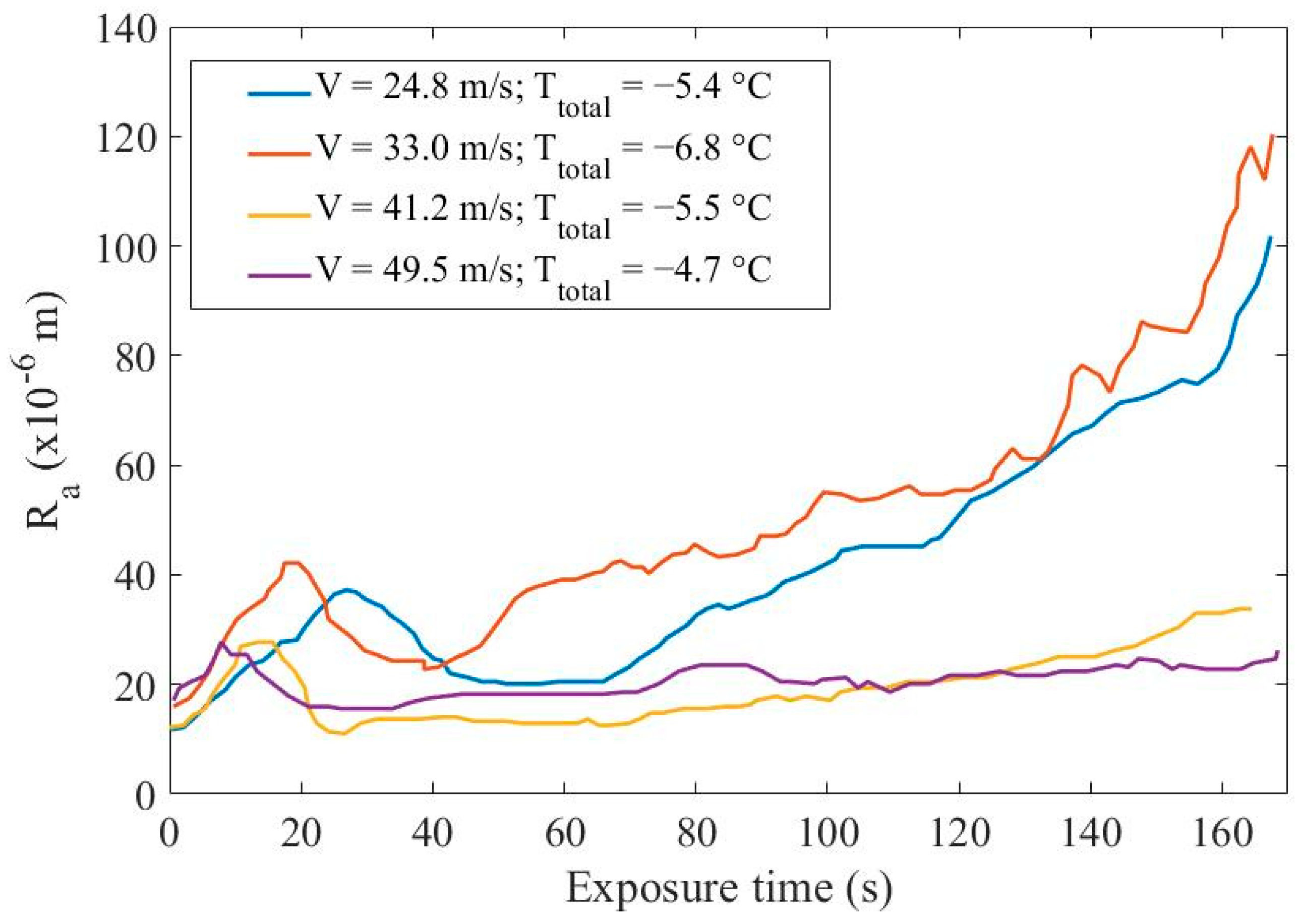
Both heat transfer and wall shear stress are functions of the surface roughness pattern and impact the computed ice shape. The development of surface roughness in the early stages then drives the ice accretion process [100]. This surface roughness is usually uncertain, both in space and time, raising a difficulty to correctly model it. Experimental measurements using photogrammetry and 3D scanning highlight a spatial variation of the roughness, with a smoother zone around the stagnation point [49,101]. Additional studies allow the monitoring of the temporal evolution of the roughness characteristics [102]. To highlight the spatial roughness variation, the experimental measurements from Han and Palacios [101] were conducted on a NACA0012 airfoil and Baghel et al. [49] used the High Altitude Pseudo Satellites (HAPS) airfoil. Variation of measured experimental Ra (Equation (1)) and Rq (Equation (2)) against the chord fraction on the upper part of the airfoil are shown in Figure 6. The x-axis origin corresponds to the stagnation point location. Figure 7 highlights the temporal roughness variation obtained on a 0.33 m chord, 0.3 m span NACA0012 wing at −5° angle of attack [102]. Figure 7 plots Ra (Equation (1)) against the exposure time for various freestream velocities (V) and total temperatures (Ttotal). Figure 6 and Figure 7 also give indications on the magnitude of roughness height usually encountered in aircraft ice accretion. This surface roughness only characterizes the very first moments of the ice accretion. The roughness models the surface irregularities of size similar to the boundary layer thickness. The ice then grows on the rough airfoil, driven by the heat transfer and shear stress, and can reach large size and thickness. In the case of ice accretions larger than the boundary layer thickness, strategies such as geometry update [103] or the immersed boundary method [104] are required to account for the wall macroscopic deformation. The multi-layer approach allows updating the airflow during the simulation, as the accretion is computed layer by layer. In most cases, the single layer approach is preferred. The single layer approach only relies on the initial flow field obtained on the rough airfoil without any large ice accretion. In some cases, the single and multi-layer approach can lead to similar results [47].
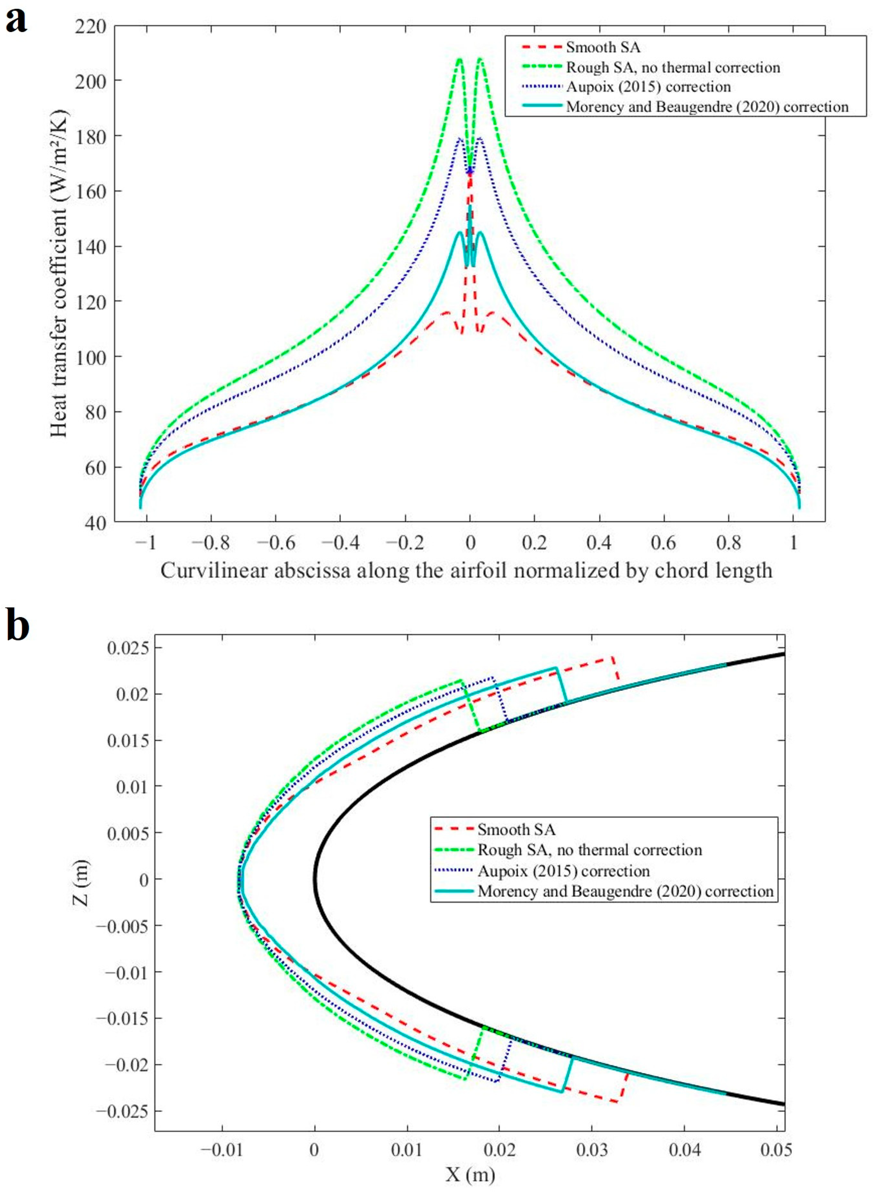
Figure 8 illustrates the influence of the thermal correction model on the ice shape in numerical simulations. Figure 8 highlights how the changes in the heat transfer coefficient (Equation (33)), resulting from the thermal correction chosen, impact the final ice shape on a NACA0012 airfoil in glaze conditions [105]. The results are presented for the smooth SA turbulence model [19], the rough SA without thermal correction [21], the rough SA with the Aupoix thermal correction [25], and for the rough SA with Morency and Beaugendre thermal correction [23].
Given the uncertainty and complex roughness patterns in the experimental setups, empirical correlations were developed to take surface roughness into account in the numerical simulations. These correlations are reviewed in the next section.
5. Empirical Roughness Correlations in Ice Accretion Simulations
Usual roughness correlations developed for sand grain paper, manufactured roughness elements, and more regular roughness patterns must be adjusted for irregular ice-induced roughness. Ice-specific roughness height and ESGR correlations were developed in an attempt to mimic the experimental observations. The early correlations assumed a uniform roughness pattern for the sake of simplification and kept the same roughness for all atmospheric conditions [106]. Gent et al. [107] suggested a roughness height function of the liquid water content (LWC), measuring the mass of liquid water droplet in a given volume of dry air (usually expressed in g/m3), the freestream velocity, the ambient air temperature, and the airfoil chord length c. Ruff [44] suggested a correlation for a uniform ESGR estimation. Shin and Bond [45] extended this correlation to include the dependency to the median volume diameter (MVD) of the water droplets, noticing that this dependency vanishes for MVD below 20 μm. The correlations from Ruff [44] and Shin and Bond [45] take the general form given by Equation (34). The coefficients A, B, C, and D are functions of the LWC, the freestream temperature, the freestream velocity, and the MVD (for [45] only), respectively.
Recent works by CIRA still use the Shin and Bond uniform relation to determine ks [108]. The commercial software FENSAP-ICE initially used Shin and Bond uniform correlation [46,109], or a constant user-defined ks. These uniform roughness correlations are still available in the FENSAP-ICE package and are regularly used [110]. FENSAP-ICE later received a non-uniform roughness beading model accounting for the roughness variability in space and time [111,112,113]. Li et al. [114] also developed a non-uniform roughness distribution in FENSAP-ICE, accounting for the state of the liquid water. In case of a continuous liquid film, the roughness height depends on the film height hw as in Equation (35), where g is the gravitational constant, τw is the wall shear stress, and μw is the water viscosity. In the case of scattered beads, the gravitational forces and water surface tension drive the roughness height.
Fortin et al. [115] also derived a specific roughness height correlation function of the local wall shear stress and local water film thickness. Anderson and Shin [116] also developed a non-uniform roughness height correlation, based on the local freezing fraction f. The freezing fraction is the proportion of incoming water (runback and impingement) that actually freezes in a control volume. This roughness height correlation, used in the ice accretion software LEWICE [117], is given in Equation (36).
Fortin [43] recently developed a logarithmic correlation for the ESGR height that includes the local collection efficiency β, the water latent heat of fusion Lf, the water fusion temperature T0, and the recovery temperature Trec alongside the liquid water content LWC (Equation (37)).
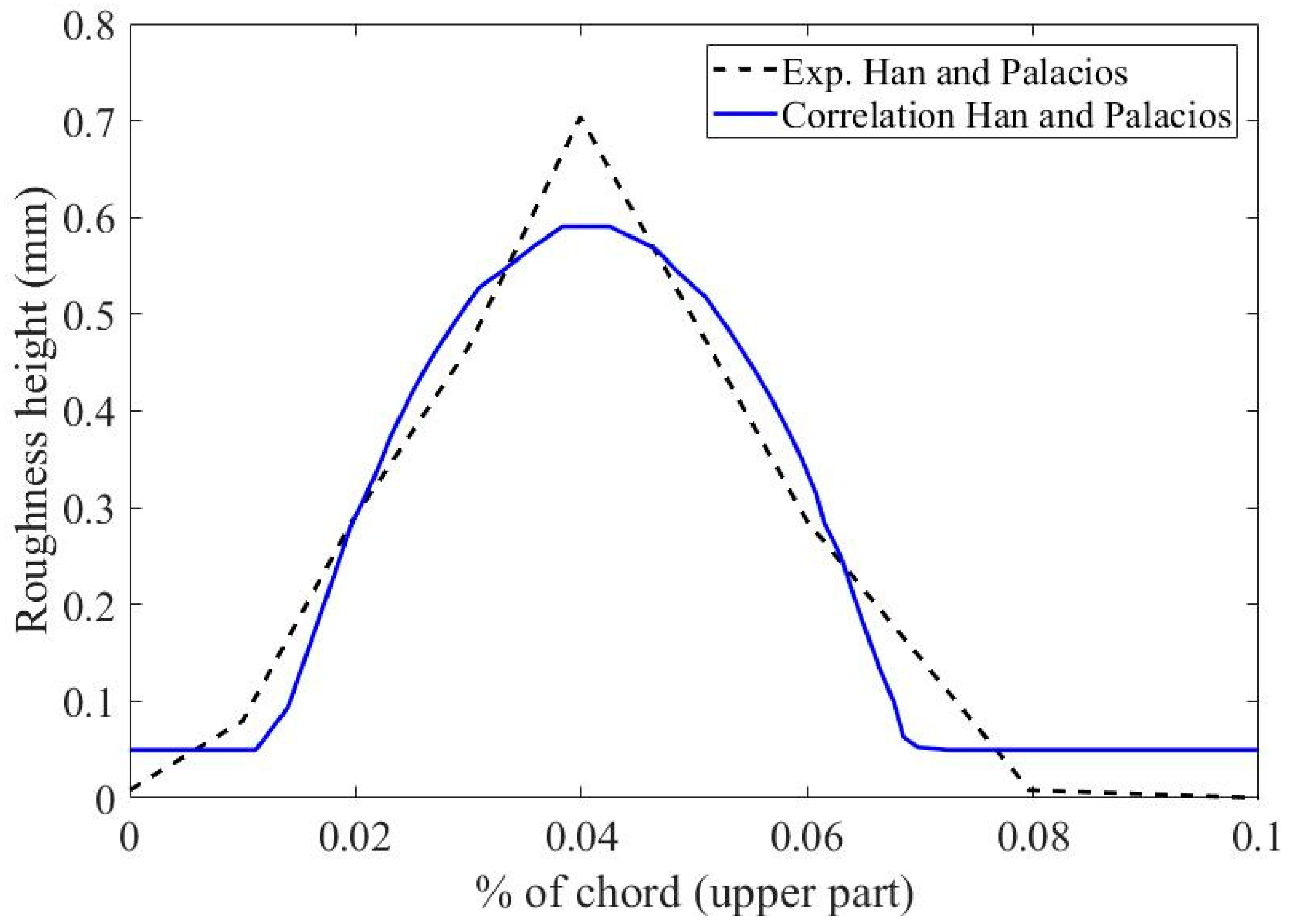
To account for the spatial variability of the roughness height, and following the LEWICE correlation (Equation (36)), Han and Palacios [50] derived a parabolic roughness distribution with respect to the wrapped distance s from the stagnation point. This correlation, with the smooth width w and the icing limit l as parameters, takes the form of Equation (38).
The parameters w, l, and kmax in Equation (38) are mainly dependent on the local freezing fraction, the accumulation parameter [50], and the airfoil leading edge radius. The correlation somehow fits the experimental roughness height, as plotted in Figure 9.
The recent advances made in ONERA with the IGLOO3D suite combine both experimental measurements and empirical correlation for the roughness estimation [41]. IGLOO3D relies on the thermal correction model from Aupoix [25] (see subsection III.B, Equations (28)–(30)). Scorr and the roughness height k are measured from experimental short-time-exposure accretions and ks is then computed using the semi-empirical correlation from Flack and Schultz [58]. The research work at NASA with the GlennICE code adopts a slightly different approach, where the roughness metric Rq is directly computed using the freezing fraction, the pressure coefficient, and the total temperature. The heat transfer coefficient is then augmented by a correction function of Rq [118].
Despite all the research efforts to develop roughness correlations for numerical simulations, existing roughness models fail to predict some experimental ice shapes. The roughness models, as well as the accretion models, are probably not universal and their results depend on both test case and code used [47,51]. Data-driven calibration methods and uncertainty quantification techniques are emerging solutions that could establish roughness patterns specifically tailored for a given case/code configuration. Such methods are already used for roughness estimation in other engineering fields [119]. Up to recently, only a few published works utilize the methods to calibrate roughness patterns for ice accretion prediction. Although the calibrated roughness patterns lack universality, the methods open new perspectives for future investigations of roughness models and their impact on ice shapes.
6. Conclusions
This paper reviewed how roughness is tackled in wall resolved RANS and the representation of surface roughness in ice accretion simulations. Focusing on the RANS turbulence models with equivalent sand grain roughness (ESGR) approach, the survey established that specific adjustments are required for realistic predictions of both heat transfer and skin friction over surface roughness. These requirements are justified by the boundary layer flow modification induced by roughness, especially the viscous sub-layer. Semi-empirical correlations were developed through decades to model the roughness geometry and ease its addition in the CFD models. The ice accretion phenomenon is a particular case of a rough surface, where the roughness pattern is highly uncertain, irregular, and difficult to measure. Ice accretion simulation codes need to account for ice roughness. Several icing-specific correlations relate roughness parameters to various atmospheric conditions and local ice properties on surfaces. The most complex correlations attempt to predict the roughness variability in space and time. A research gap was highlighted, showing that the roughness correlations may fail to predict correct ice shapes in some cases. This opens the perspective of using uncertainty quantification tools to improve the roughness pattern prediction for ice accretion simulations and detach the roughness estimation from the historical semi-empirical correlations. As a recommendation, other gaps still need attention such as a better understanding of the roughness time evolution.
Funding
This research received no external funding.
Acknowledgments
The authors want to thank the TOMATO Association (Aéroclub de France), Paris, France, the Office of the Dean of Studies, ÉTS, Montréal, Canada, and SubstanceETS, Montréal, Canada. CFD computations were carried out on the supercomputer Cedar from Simon Fraser University. This research was enabled in part by support provided by Calcul Québec and the Digital Research Alliance of Canada (alliancecan.ca (accessed on 1 August 2023)).
Conflicts of Interest
The authors declare no conflict of interest.
References
- Gao, H.; Li, X.; Nezhad, A.H.; Behshad, A. Numerical simulation of the flow in pipes with numerical models. Struct. Eng. Mech. 2022, 81, 523–527. [Google Scholar] [CrossRef]
- Marquet, O.; Leontini, J.S.; Zhao, J.; Thompson, M.C. Hysteresis of two-dimensional flows around a NACA0012 airfoil at Re=5000 and linear analyses of their mean flow. Int. J. Heat Fluid Flow 2022, 94, 108920. [Google Scholar] [CrossRef]
- Howell, J.; Forbes, D.; Passmore, M.; Page, G. The Effect of a Sheared Crosswind Flow on Car Aerodynamics. SAE Int. J. Passeng. Cars-Mech. Systems 2017, 10, 278–285. [Google Scholar] [CrossRef]
- Jafari, M.; Alipour, A. Review of approaches, opportunities, and future directions for improving aerodynamics of tall buildings with smart facades. Sustain. Cities Soc. 2021, 72, 102979. [Google Scholar] [CrossRef]
- Kaya, M.N.; Kok, A.R.; Kurt, H. Comparison of aerodynamic performances of various airfoils from different airfoil families using CFD. Wind. Struct. Int. J. 2021, 32, 239–248. [Google Scholar] [CrossRef]
- Omoware, W.D.; Maheri, A.; Azimov, U. Aerodynamic analysis of flapping-pitching flat plates. In Proceedings of the 3rd International Symposium on Environmental Friendly Energies and Applications (EFEA), Paris, France, 19–21 November 2014; pp. 1–5. [Google Scholar] [CrossRef]
- Bons, J.P. A review of surface roughness effects in gas turbines. J. Turbomach. 2010, 132, 021004. [Google Scholar] [CrossRef]
- Kontogiannis, A.; Prakash, A.; Laurendeau, E.; Moens, F. Sensitivity of Glaze Ice Accretion and Iced Aerodynamics Prediction to Roughness. In Proceedings of the 26th Annual Conference of the Computational Fluid Dynamics Society of Canada, Winnipeg, MB, Canada, 10–12 June 2018. [Google Scholar]
- Hosni, M.H.; Coleman, H.W.; Garner, J.W.; Taylor, R.P. Roughness element shape effects on heat transfer and skin friction in rough-wall turbulent boundary layers. Int. J. Heat Mass Transf. 1993, 36, 147–153. [Google Scholar] [CrossRef]
- Kadivar, M.; Tormey, D.; McGranaghan, G. A review on turbulent flow over rough surfaces: Fundamentals and theories. Int. J. Thermofluids 2021, 10, 100077. [Google Scholar] [CrossRef]
- Suga, K.; Craft, T.J.; Iacovides, H. An analytical wall-function for turbulent flows and heat transfer over rough walls. Int. J. Heat Fluid Flow 2006, 27, 852–866. [Google Scholar] [CrossRef]
- Schlichting, H. Experimental Investigation of the Problem of Surface Roughness; NACA-TM-823; National Advisory Commitee for Aeronautics: Edwards, CA, USA, 1937. [Google Scholar]
- Botros, K.K. Experimental Investigation into the Relationship between the Roughness Height in Use with Nikuradse or Colebrook Roughness Functions and the Internal Wall Roughness Profile for Commercial Steel Pipes. J. Fluids Eng. Trans. ASME 2016, 138, 081202. [Google Scholar] [CrossRef]
- Javanappa, S.K.; Narasimhamurthy, V.D. DNS of plane Couette flow with surface roughness. Int. J. Adv. Eng. Sci. Appl. Math. 2019, 11, 288–300. [Google Scholar] [CrossRef]
- Forooghi, P.; Stroh, A.; Schlatter, P.; Frohnapfel, B. Direct numerical simulation of flow over dissimilar, randomly distributed roughness elements: A systematic study on the effect of surface morphology on turbulence. Phys. Rev. Fluids 2018, 3, 044605. [Google Scholar] [CrossRef]
- Rao, V.N.; Jefferson-Loveday, R.; Tucker, P.G.; Lardeau, S. Large eddy simulations in turbines: Influence of roughness and free-stream turbulence. Flow Turbul. Combust. 2014, 92, 543–561. [Google Scholar] [CrossRef]
- De Marchis, M. Large eddy simulations of roughened channel flows: Estimation of the energy losses using the slope of the roughness. Comput. Fluids 2016, 140, 148–157. [Google Scholar] [CrossRef]
- Blazek, J. Computational Fluid Dynamics: Principles and Applications, 2nd ed.; Elsevier: Amsterdam, The Netherlands, 2005. [Google Scholar]
- Spalart, P.; Allmaras, S. A one-equation turbulence model for aerodynamic flows. In 30th Aerospace Sciences Meeting and Exhibit; American Institute of Aeronautics and Astronautics: Reston, VA, USA, 1992. [Google Scholar] [CrossRef]
- Menter, F.R. Two-equation eddy-viscosity turbulence models for engineering applications. AIAA J. 1994, 32, 1598–1605. [Google Scholar] [CrossRef]
- Aupoix, B.; Spalart, P.R. Extensions of the Spalart–Allmaras turbulence model to account for wall roughness. Int. J. Heat Fluid Flow 2003, 24, 454–462. [Google Scholar] [CrossRef]
- Chedevergne, F. A double-averaged Navier-Stokes k -ω turbulence model for wall flows over rough surfaces with heat transfer. J. Turbul. 2021, 22, 713–734. [Google Scholar] [CrossRef]
- Morency, F.; Beaugendre, H. Comparison of turbulent Prandtl number correction models for the Stanton evaluation over rough surfaces. Int. J. Comput. Fluid Dyn. 2020, 34, 278–298. [Google Scholar] [CrossRef]
- Chedevergne, F. Analytical wall function including roughness corrections. Int. J. Heat Fluid Flow 2018, 73, 258–269. [Google Scholar] [CrossRef]
- Aupoix, B. Improved heat transfer predictions on rough surfaces. Int. J. Heat Fluid Flow 2015, 56, 160–171. [Google Scholar] [CrossRef]
- Hanson, D.R.; Kinzel, M.P.; McClain, S.T. Validation of the discrete element roughness method for predicting heat transfer on rough surfaces. Int. J. Heat Mass Transf. 2019, 136, 1217–1232. [Google Scholar] [CrossRef]
- Hanson, D.R.; Kinzel, M.P. Application of the discrete element roughness method to ice accretion geometries. In Proceedings of the 46th AIAA Fluid Dynamics Conference, Washington, DC, USA, 13–17 June 2016; American Institute of Aeronautics and Astronautics Inc, AIAA: Las Vegas, NV, USA, 2016. [Google Scholar]
- Aupoix, B. Revisiting the Discrete Element Method for Predictions of Flows over Rough Surfaces. J. Fluids Eng. Trans. ASME 2016, 138, 031205. [Google Scholar] [CrossRef]
- Chedevergne, F. Modeling rough walls from surface topography to double averaged Navier-Stokes computation. J. Turbul. 2023, 24, 36–56. [Google Scholar] [CrossRef]
- Jayabarathi, S.B.; Ratnam, M.M. Comparison of Correlation between 3D Surface Roughness and Laser Speckle Pattern for Experimental Setup Using He-Ne as Laser Source and Laser Pointer as Laser Source. Sensors 2022, 2, 6003. [Google Scholar] [CrossRef] [PubMed]
- Mejia-Alvarez, R.; Christensen, K.T. Wall-parallel stereo particle-image velocimetry measurements in the roughness sublayer of turbulent flow overlying highly irregular roughness. Phys. Fluids 2013, 25, 115109. [Google Scholar] [CrossRef]
- Kuwata, Y.; Yamamoto, Y.; Tabata, S.; Suga, K. Scaling of the roughness effects in turbulent flows over systematically-varied irregular rough surfaces. Int. J. Heat Fluid Flow 2023, 101, 109130. [Google Scholar] [CrossRef]
- Leach, R. Characterisation of Areal Surface Texture, 1st ed.; Leach, R., Ed.; Springer: Berlin/Heidelberg, Germany, 2013; p. 353. [Google Scholar] [CrossRef]
- Nikuradse, J. Laws of flow in rough pipes. VDI Forschungsheft 1933, 4, 63. [Google Scholar]
- Dirling, R. A method for computing roughwall heat transfer rates on reentry nosetips. In Proceedings of the 8th Thermophysics Conference, Palm Springs, CA, USA, 16–18 July 1973. [Google Scholar] [CrossRef]
- Sigal, A.; Danberg, J.E. New correlation of roughness density effect on the turbulent boundary layer. AIAA J. 1990, 28, 554–556. [Google Scholar] [CrossRef]
- McClain, S.T.; Vargas, M.; Jen-Ching, T. Characterization of Ice Roughness Variations in Scaled Glaze Icing Conditions. In Proceedings of the 8th AIAA Atmospheric and Space Environments Conference, Reston, VA, USA, 13–17 June 2016; AIAA—American Institute of Aeronautics and Astronautics: Reston, VA, USA, 2016; p. 14. [Google Scholar]
- Liu, Y.; Hu, H. An experimental investigation on the unsteady heat transfer process over an ice accreting airfoil surface. Int. J. Heat Mass Transf. 2018, 122, 707–718. [Google Scholar] [CrossRef]
- Bourgault-Cote, S.; Docampo-Sánchez, J.; Laurendeau, E. Multi-Layer Ice Accretion Simulations Using a Level-Set Method with B-Spline Representation. In Proceedings of the 2018 AIAA Aerospace Sciences Meeting, Kissimmee, FL, USA, 8–12 January 2018. [Google Scholar]
- Akbal, O.; Ayan, E.; Murat, C.; Ozgen, S. Flight Ice Shape Prediction with Data Fit Surrogate Models; SAE International: Minneapolis, MN, USA, 2023. [Google Scholar] [CrossRef]
- Radenac, E.; Gaible, H.; Bezard, H.; Reulet, P. IGLOO3D Computations of the Ice Accretion on Swept-Wings of the SUNSET2 Database. In Proceedings of the International Conference on Icing of Aircraft, Engines, and Structures, Minneapolis, MN, USA, 17–21 June 2019; SAE International: Minneapolis, MN, USA, 2019. [Google Scholar] [CrossRef]
- Shannon, T.; McClain, S.T. An Assessment of LEWICE Roughness and Convection Enhancement Models. SAE Int. J. Adv. Curr. Pract. Mobil. 2019, 2, 128–139. [Google Scholar] [CrossRef]
- Fortin, G. Equivalent Sand Grain Roughness Correlation for Aircraft Ice Shape Predictions; SAE International: Minneapolis, MN, USA, 2019. [Google Scholar] [CrossRef]
- Ruff, G.A.; Berkowitz, B.M. Users Manual for the NASA Lewis Ice Accretion Prediction Code (LEWICE); NASA CR-185129; National Aeronautics and Space Administration: Washington, DC, USA, 1990. [Google Scholar]
- Shin, J.; Bond, T.H. Results of an icing test on a NACA 0012 airfoil in the NASA Lewis Icing Research Tunnel. In Proceedings of the 30th Aerospace Sciences Meeting and Exhibit, Reno, NV, USA, 6–9 January 1992. [Google Scholar] [CrossRef]
- Shin, J.; Berkowitz, B.; Chen, H.H.; Cebeci, T. Prediction of ice shapes and their effect on airfoil performance. In Proceedings of the AIAA 29th Aerospace Sciences Meeting, Reno, NV, USA, 7–10 January 1991. [Google Scholar]
- Lavoie, P.; Pena, D.; Hoarau, Y.; Laurendeau, E. Comparison of thermodynamic models for ice accretion on airfoils. Int. J. Numer. Methods Heat Fluid Flow 2018, 28, 1004–1030. [Google Scholar] [CrossRef]
- Hansman, R.; Yamaguchi, K.; Berkowitz, B.; Potapczuk, M. Modeling of Surface Roughness Effects on Glaze Ice Accretion. J. Thermophys. Heat Transf. 1989, 5, 54–60. [Google Scholar] [CrossRef]
- Baghel, A.P.; Sotomayor-Zakharov, D.; Knop, I.; Ortwein, H.-P. Detailed Study of Photogrammetry Technique as a Valid Ice Accretion Measurement Method; SAE International: Minneapolis, MN, USA, 2023. [Google Scholar] [CrossRef]
- Han, Y.; Palacios, J. Surface Roughness and Heat Transfer Improved Predictions for Aircraft Ice-Accretion Modeling. AIAA J. 2017, 55, 1318–1331. [Google Scholar] [CrossRef]
- Laurendeau, E.; Bourgault-Cote, S.; Ozcer, I.A.; Hann, R.; Radenac, E.; Pueyo, A. Summary from the 1st AIAA Ice Prediction Workshop. In Proceedings of the AIAA AVIATION 2022 Forum, Chicago, IL, USA, 27 June–1 July 2022. [Google Scholar] [CrossRef]
- Caccia, F.; Guardone, A. Numerical simulations of ice accretion on wind turbine blades: Are performance losses due to ice shape or surface roughness? Wind. Energy Sci. 2023, 8, 341–362. [Google Scholar] [CrossRef]
- Ravenna, R.; Song, S.; Shi, W.; Sant, T.; De Marco Muscat-Fenech, C.; Tezdogan, T.; Demirel, Y.K. CFD analysis of the effect of heterogeneous hull roughness on ship resistance. Ocean. Eng. 2022, 258, 111733. [Google Scholar] [CrossRef]
- Committee, S.E. Surface Texture; SAE International: Warrendale, PA, USA, 2023. [Google Scholar] [CrossRef]
- Leach, R. Introduction to Surface Topography. In Characterisation of Areal Surface Texture; Leach, R., Ed.; Springer: Berlin/Heidelberg, Germany, 2013; pp. 1–13. [Google Scholar] [CrossRef]
- Heldt, E. Measurement of component surface roughness. Qual. Und Zuverlaessigkeit 2006, 51, 80–84. [Google Scholar]
- Todhunter, L.D.; Leach, R.K.; Lawes, S.D.A.; Blateyron, F. Industrial survey of ISO surface texture parameters. CIRP J. Manuf. Sci. Technol. 2017, 19, 84–92. [Google Scholar] [CrossRef]
- Flack, K.A.; Schultz, M.P. Review of Hydraulic Roughness Scales in the Fully Rough Regime. J. Fluids Eng. 2010, 132, 041203. [Google Scholar] [CrossRef]
- Schlichting, H.; Gersten, K. Boundary-Layer Theory, 9th ed.; Springer: Berlin/Heidelberg, Germany, 2017. [Google Scholar] [CrossRef]
- van Rij, J.A.; Belnap, B.J.; Ligrani, P.M. Analysis and Experiments on Three-Dimensional, Irregular Surface Roughness. J. Fluids Eng. 2002, 124, 671–677. [Google Scholar] [CrossRef]
- Colebrook, C.F.; White, C.M.; Taylor, G.I. Experiments with fluid friction in roughened pipes. Proc. R. Soc. London. Ser. A-Math. Phys. Sci. 1937, 161, 367–381. [Google Scholar] [CrossRef]
- Bons, J.P. St and cf Augmentation for Real Turbine Roughness with Elevated Freestream Turbulence. J. Turbomach. 2002, 124, 632–644. [Google Scholar] [CrossRef]
- Von Kármán, T. Mechanical Similitude and Turbulence; NACA-TM-611; National Advisory Committee for Aeronautics: Washington, DC, USA, 1931. [Google Scholar]
- Reichardt, H. Vollständige Darstellung der turbulenten Geschwindigkeitsverteilung in glatten Leitungen. ZAMM-J. Appl. Math. Mech./Z. Für Angew. Math. Und Mech. 1951, 31, 208–219. [Google Scholar] [CrossRef]
- Heng, L.; Duo, W.; Hongyi, X. Improved Law-of-the-Wall Model for Turbulent Boundary Layer in Engineering. AIAA J. 2020, 58, 3308–3319. [Google Scholar] [CrossRef]
- Ghanadi, F.; Djenidi, L. Study of a rough-wall turbulent boundary layer under pressure gradient. J. Fluid Mech. 2022, 938, A17. [Google Scholar] [CrossRef]
- Ligrani, P.M.; Moffat, R.J. Structure of transitionally rough and fully rough turbulent boundary layers. J. Fluid Mech. 1986, 162, 69–98. [Google Scholar] [CrossRef]
- Langelandsvik, L.I.; Kunkel, G.; Smits, A. Flow in a commercial steel pipe. J. Fluid Mech. 2008, 595, 323–339. [Google Scholar] [CrossRef]
- Schultz, M.P.; Flack, K.A. The rough-wall turbulent boundary layer from the hydraulically smooth to the fully rough regime. J. Fluid Mech. 2007, 580, 381–405. [Google Scholar] [CrossRef]
- Wilcox, D.C. Turbulence Modeling for CFD; DCW Industries: La Cañada Flintridge, CA, USA, 2006. [Google Scholar]
- Patel, V.C.; Yoon, J.Y. Application of Turbulence Models to Separated Flow Over Rough Surfaces. J. Fluids Eng. 1995, 117, 234–241. [Google Scholar] [CrossRef]
- Hellsten, A.; Laine, S. Extension of the k-omega-SST turbulence model for flows over rough surfaces. In Proceedings of the AIAA 22nd Atmospheric Flight Mechanics Conference, New Orleans, LA, USA, 11–13 August 1997. [Google Scholar]
- Knopp, T.; Eisfeld, B.; Calvo, J.B. A new extension for k–ω turbulence models to account for wall roughness. Int. J. Heat Fluid Flow 2009, 30, 54–65. [Google Scholar] [CrossRef]
- Durbin, P.A.; Medic, G.; Seo, J.M.; Eaton, J.K.; Song, S. Rough wall modification of two-layer k-ε. Trans. ASME J. Fluids Eng. 2001, 123, 16–21. [Google Scholar] [CrossRef]
- Kays, W.M.; Crawford, M.E. Convective Heat and Mass Transfer; McGraw-Hill: New York, NY, USA, 1993. [Google Scholar]
- Grigson, C. Drag Losses of New Ships Caused by Hull Finish. J. Ship Res. 1992, 36, 182–196. [Google Scholar] [CrossRef]
- Radenac, E.; Kontogiannis, A.; Bayeux, C.; Villedieu, P. An extended rough-wall model for an integral boundary layer model intended for ice accretion calculations. In Proceedings of the 2018 Atmospheric and Space Environments Conference, AIAA, Atlanta, GA, USA, 25–29 June 2018. [Google Scholar] [CrossRef]
- Orych, M.; Werner, S.; Larsson, L. Roughness effect modelling for wall resolved RANS—Comparison of methods for marine hydrodynamics. Ocean. Eng. 2022, 266, 112778. [Google Scholar] [CrossRef]
- Andersson, J.; Oliveira, D.R.; Yeginbayeva, I.; Leer-Andersen, M.; Bensow, R.E. Review and comparison of methods to model ship hull roughness. Appl. Ocean. Res. 2020, 99, 102119. [Google Scholar] [CrossRef]
- Ligrani, P.M.; Moffat, R.J.; Kays, W.M. The Thermal and Hydrodynamic Behavior of Thick, Rough-Wall, Turbulent Boundary Layers; Stanford University: Stanford, CA, USA, 1979. [Google Scholar]
- Dipprey, D.F.; Sabersky, R.H. Heat and momentum transfer in smooth and rough tubes at various prandtl numbers. Int. J. Heat Mass Transf. 1963, 6, 329–353. [Google Scholar] [CrossRef]
- Owen, P.R.; Thomson, W.R. Heat transfer across rough surfaces. J. Fluid Mech. 1963, 15, 321–334. [Google Scholar] [CrossRef]
- International Air Transport Association. Safety Report 2015; International Air Transport Association: Montreal, QC, Canada, 2016. [Google Scholar]
- Cao, Y.; Tan, W.; Wu, Z. Aircraft icing: An ongoing threat to aviation safety. Aerosp. Sci. Technol. 2018, 75, 353–385. [Google Scholar] [CrossRef]
- Bragg, M.B.; Broeren, A.P.; Blumenthal, L.A. Iced-airfoil aerodynamics. Prog. Aerosp. Sci. 2005, 41, 323–362. [Google Scholar] [CrossRef]
- Esmaeilifar, E.; Prince Raj, L.; Myong, R.S. Computational simulation of aircraft electrothermal de-icing using an unsteady formulation of phase change and runback water in a unified framework. Aerosp. Sci. Technol. 2022, 130, 107936. [Google Scholar] [CrossRef]
- Bennani, L.; Villedieu, P.; Salaun, M.; Trontin, P. Numerical simulation and modeling of ice shedding: Process initiation. Comput. Struct. 2014, 142, 15–27. [Google Scholar] [CrossRef]
- Ignatowicz, K.; Morency, F.; Lopez, P. Dynamic Moment Model for Numerical Simulation of a 6-DOF Plate Trajectory around an Aircraft. J. Aerosp. Eng. 2019, 32. [Google Scholar] [CrossRef]
- Dukhan, N.; Masiulaniec, K.C.; Witt, K.J.D.; Fossen, G.J.V. Experimental Heat Transfer Coefficients from Ice-Roughened Surfaces for Aircraft Deicing Design. J. Aircr. 1999, 36, 948–956. [Google Scholar] [CrossRef]
- Gori, G.; Bellosta, T.; Guardone, A. Numerical Simulation of In-Flight Icing Under Uncertain Conditions. In Handbook of Numerical Simulation of In-Flight Icing; Habashi, W.G., Ed.; Springer International Publishing: Cham, Switzerland, 2023; pp. 1–34. [Google Scholar] [CrossRef]
- Fujiwara, G.E.C.; Bragg, M.B.; Broeren, A.P. Comparison of Computational and Experimental Ice Accretions of Large Swept Wings. J. Aircr. 2020, 57, 342–359. [Google Scholar] [CrossRef]
- Messinger, B.L. Equilibrium Temperature of an Unheated Icing Surface as a Function of Air Speed. J. Aeronaut. Sci. 1953, 20, 29–42. [Google Scholar] [CrossRef]
- Myers, T.G. Extension to the Messinger Model for Aircraft Icing. AIAA J. 2001, 39, 211–218. [Google Scholar] [CrossRef]
- Zhu, C.; Fu, B.; Sun, Z.; Zhu, C. 3D Ice Accretion Simulation For Complex Configuration Basing On Improved Messinger Model. Int. J. Mod. Phys. Conf. Ser. 2012, 19, 341–350. [Google Scholar] [CrossRef]
- Ayan, E.; Ozgen, S. Modification of the Extended Messinger Model for Mixed Phase Icing and Industrial Applications with TAICE. In Proceedings of the 9th AIAA Atmospheric and Space Environments Conference, Denver, CO, USA, 5–9 June 2017; p. 3759. [Google Scholar]
- Bourgault, Y.; Beaugendre, H.; Habashi, W.G. Development of a Shallow-Water Icing Model in FENSAP-ICE. J. Aircr. 2000, 37, 640–646. [Google Scholar] [CrossRef]
- Ignatowicz, K.; Morency, F.; Beaugendre, H. Extension of SU2 CFD capabilities to 3D aircraft icing simulation. In Proceedings of the 29th Annual Conference of the Computational Fluid Dynamics Society of Canada (CFDSC2021), Online, 27–29 July 2021. [Google Scholar]
- Özgen, S.; Canıbek, M. Ice accretion simulation on multi-element airfoils using extended Messinger model. Heat Mass Transf. 2008, 45, 305. [Google Scholar] [CrossRef]
- Macarthur, C.; Keller, J.; Luers, J. Mathematical modeling of ice accretion on airfoils. In Proceedings of the 20th Aerospace Sciences Meeting, Orlando, FL, USA, 11–14 January 1982. [Google Scholar] [CrossRef]
- Liu, Y.; Zhang, K.; Tian, W.; Hu, H. An experimental investigation on the dynamic ice accretion and unsteady heat transfer over an airfoil surface with embedded initial ice roughness. Int. J. Heat Mass Transf. 2020, 146, 118900. [Google Scholar] [CrossRef]
- Han, Y.; Palacios, J. Transient Heat Transfer Measurements of Surface Roughness due to Ice Accretion. In Proceedings of the 6th AIAA Atmospheric and Space Environments Conference, Reston, VA, USA, 16–20 June 2014; p. 22. [Google Scholar]
- Wang, Y.; Zhang, Y.; Wang, Y.; Zhu, D.; Zhao, N.; Zhu, C. Quantitative Measurement Method for Ice Roughness on an Aircraft Surface. Aerospace 2022, 9, 739. [Google Scholar] [CrossRef]
- Fossati, M.; Khurram, R.A.; Habashi, W.G. An ALE mesh movement scheme for long-term in-flight ice accretion. Int. J. Numer. Methods Fluids 2012, 68, 958–976. [Google Scholar] [CrossRef]
- de Rosa, D.; Capizzano, F.; Cinquegrana, D. Multi-Step Ice Accretion by Immersed Boundaries; SAE International: Minneapolis, MN, USA, 2023. [Google Scholar] [CrossRef]
- Ignatowicz, K.; Morency, F.; Beaugendre, H. Numerical simulation of ice accretion using Messinger-based approach: Effects of surface roughness. In Proceedings of the CASI AERO 2019, CASI, Laval, QC, Canada, 14–16 May 2019. [Google Scholar]
- Wright, W.B.; Gent, R.W.; Guffond, D. DRA/NASA/ONERA Collaboration on Icing Research. Part II—Prediction of Airfoil Ice Accretion; NASA: Washington, DC, USA, 1997. [Google Scholar]
- Gent, R.; Markiewicz, R.; Cansdale, J. Further Studies of Helicopter Rotor Ice Accretion and Protection. Vertica 1987, 11, 473–492. [Google Scholar]
- Cinquegrana, D.; D’Aniello, F.; de Rosa, D.; Carozza, A.; Catalano, P.; Mingione, G. A CIRA 3D Ice Accretion Code for Multiple Cloud Conditions Simulations; SAE International: Minneapolis, MN, USA, 2023. [Google Scholar] [CrossRef]
- Beaugendre, H.; Morency, F.; Habashi, W.G.; Benquet, P. Roughness Implementation in FENSAP-ICE: Model Calibration and Influence on Ice Shapes. J. Aircr. 2003, 40, 1212–1215. [Google Scholar] [CrossRef]
- Martini, F.; Ibrahim, H.; Contreras Montoya, L.T.; Rizk, P.; Ilinca, A. Turbulence Modeling of Iced Wind Turbine Airfoils. Energies 2022, 15, 8325. [Google Scholar] [CrossRef]
- Ozcer, I.A.; Baruzzi, G.S.; Reid, T.; Habashi, W.G.; Fossati, M.; Croce, G. FENSAP-ICE: Numerical Prediction of Ice Roughness Evolution, and Its Effects on Ice Shapes; SAE International: Minneapolis, MN, USA, 2011. [Google Scholar] [CrossRef]
- Croce, G.; Candido, E.D.; Habashi, W.; Aubé, M.; Baruzzi, G. FENSAP-ICE: Numerical Prediction of In-flight Icing Roughness Evolution. In Proceedings of the 1st AIAA Atmospheric and Space Environments Conference, San Antonio, TX, USA, 22–25 June 2009. [Google Scholar] [CrossRef]
- ANSYS. ANSYS FENSAP-ICE User Manual; ANSYS: Canonsburg, PA, USA, 2020. [Google Scholar]
- Yan, L.; Chao, W.; Shi-nan, C.; Du, C. Simulation of Ice Accretion Based on Roughness Distribution. Procedia Eng. 2011, 17, 160–177. [Google Scholar] [CrossRef]
- Fortin, G.; Laforte, J.-L.; Ilinca, A. Heat and mass transfer during ice accretion on aircraft wings with an improved roughness model. Int. J. Therm. Sci. 2006, 45, 595–606. [Google Scholar] [CrossRef]
- Anderson, D.; Shin, J.; Anderson, D.; Shin, J. Characterization of ice roughness from simulated icing encounters. In Proceedings of the AIAA 35th Aerospace Sciences Meeting and Exhibit, Reno, NV, USA, 6–9 January 1997. [Google Scholar] [CrossRef]
- Wright, W. User’s Manual for LEWICE Version 3.2; QSS Group, Inc.: Cleveland, OH, USA, 2008. [Google Scholar]
- Wright, W.; Rigby, D.; Ozoroski, T. Roughness Parameter Optimization of the McClain Model in GlennICE; SAE International: Minneapolis, MN, USA, 2023. [Google Scholar] [CrossRef]
- Aghaei Jouybari, M.; Junlin, Y.; Brereton, G.J.; Murillo, M.S. Data-driven prediction of the equivalent sand-grain height in rough-wall turbulent flows. J. Fluid Mech. 2021, 912, A8. [Google Scholar] [CrossRef]
Figure 1.
(A) Example of rough area, with fluid flowing above, and (B) a rough profile with the usual metrics.
Figure 1.
(A) Example of rough area, with fluid flowing above, and (B) a rough profile with the usual metrics.

Figure 2.
(A) Hydraulically smooth; (B) Transitionally rough; and (C) Fully rough. The dashed line corresponds to the viscous sublayer thickness and the solid line represents the rough surface.
Figure 2.
(A) Hydraulically smooth; (B) Transitionally rough; and (C) Fully rough. The dashed line corresponds to the viscous sublayer thickness and the solid line represents the rough surface.


Figure 4.
Illustration of the trapped fluid between roughness elements.

Figure 5.
Typical control volume for ice accretion simulations.

Figure 6.
Experimental spatial roughness measurements from Han and Palacios [101] and Baghel et al. [49].

Figure 7.
Experimental roughness temporal evolution measurements [102].
Figure 7.
Experimental roughness temporal evolution measurements [102].

Figure 8.
(a) Heat transfer coefficient for different models [19,21,23,25]; and (b) Resulting ice shapes [105].

Figure 9.
Parabolic correlation from Han and Palacios [50] (Equation (38)).
Figure 9.
Parabolic correlation from Han and Palacios [50] (Equation (38)).


Disclaimer/Publisher’s Note: The statements, opinions and data contained in all publications are solely those of the individual author(s) and contributor(s) and not of MDPI and/or the editor(s). MDPI and/or the editor(s) disclaim responsibility for any injury to people or property resulting from any ideas, methods, instructions or products referred to in the content. |
© 2023 by the authors. Licensee MDPI, Basel, Switzerland. This article is an open access article distributed under the terms and conditions of the Creative Commons Attribution (CC BY) license (https://creativecommons.org/licenses/by/4.0/).
Share and Cite
MDPI and ACS Style
Ignatowicz, K.; Morency, F.; Beaugendre, H. Surface Roughness in RANS Applied to Aircraft Ice Accretion Simulation: A Review. Fluids 2023, 8, 278. https://doi.org/10.3390/fluids8100278
AMA Style
Ignatowicz K, Morency F, Beaugendre H. Surface Roughness in RANS Applied to Aircraft Ice Accretion Simulation: A Review. Fluids. 2023; 8(10):278. https://doi.org/10.3390/fluids8100278
Chicago/Turabian StyleIgnatowicz, Kevin, François Morency, and Héloïse Beaugendre. 2023. "Surface Roughness in RANS Applied to Aircraft Ice Accretion Simulation: A Review" Fluids 8, no. 10: 278. https://doi.org/10.3390/fluids8100278