
Investigation of Flow-Induced Instabilities in a Francis Turbine Operating in Non-Cavitating and Cavitating Part-Load Conditions

Mechanics and Maritime Sciences, Chalmers University of Technology, 412 96 Gothenburg, Sweden
*
Author to whom correspondence should be addressed.
Fluids 2023, 8(2), 61; https://doi.org/10.3390/fluids8020061
Submission received: 13 January 2023
/
Revised: 31 January 2023
/
Accepted: 4 February 2023
/
Published: 10 February 2023
(This article belongs to the Special Issue Recent Advances in Fluid Mechanics: Feature Papers, 2022)
Abstract
:The integration of intermittent renewable energy resources to the grid system requires that hydro turbines regularly operate at part-load conditions. Reliable operation of hydro turbines at these conditions is typically limited by the formation of a Rotating Vortex Rope (RVR) in the draft tube. In this paper, we investigate the formation of this vortex using the scale-resolving methods SST-SAS, wall-modeled LES (WMLES), and zonal WMLES. The numerical results are first validated against the available experimental data, and then analyzed to explain the effect of using different scale-resolving methods in detail. It is revealed that although all methods can capture the main features of the RVRs, the WMLES method provides the best quantitative agreement between the simulation results and experiment. Furthermore, cavitating simulations are performed using WMLES method to study the effect of cavitation on the flow in the turbine. These effects of cavitation are shown to be highly dependent on the amount of vapor in the RVR. If the amount of vapor is small, cavitation induces broadband high-frequency fluctuations in the pressure and forces exerted on the turbine. As the amount of cavitation increases, these fluctuations tend to have a distinct dominant frequency which is different from the frequency of the RVR.
1. Introduction
Due to their large storage capacity and quick response, hydro power plants are more and more being used to facilitate the integration of intermittent energy produced by other renewable sources of energy such as wind and solar to the grid system. This requires that hydro power plants expand their range of operation and also operate frequently at off-design conditions. In such off-design operation, the flow in different components of a hydro power plant is prone to complex behaviors and instabilities. One example is the formation of a Rotating Vortex Rope (RVR) in the draft tube which is associated with a high level of pressure fluctuations in the system. These pressure fluctuations can cause oscillation in the mechanical loading of the runner, causing a significant swing in the power produced by the hydro power plant [1,2]. Furthermore, the pressure drop in the core of the RVR can lead to the formation of vapor pockets in the water flow, known as cavitation. The presence of cavitation in hydro turbines is known to have several undesirable effects, such as cavitation erosion [3], performance degradation [4], and increased level of pressure fluctuations and vibration [5].
The detrimental effects of the RVR for hydro turbines operating at off-design conditions have motivated several experimental studies with the aim to investigate the formation of the RVR and its associated cavitating structures. Nishi et al. [6] experimentally examined non-cavitating and cavitating RVRs at different flow conditions. They observed that the pressure fluctuations induced by the RVR can be decomposed into synchronous and convective components. Iliescu et al. [7] studied the dynamics of non-cavitating and cavitating RVRs using High-Speed Visualization (HSV) and Particle Image Velocimetry (PIV) measurements. They concluded that the formation of vapor pockets in an RVR can lead to fluctuations in its geometrical features. Favrel et al. [8] and Arpe et al. [9] studied the effect of cavitation on the pressure fluctuations induced by the RVR. They both concluded that cavitation formation in the RVR can influence both the amplitude and the frequency of the pressure fluctuations. Further, Landry et al. [10] showed that the presence of cavitation in the RVR can alter the eigenfrequency of the hydraulic system by changing the sound propagation speed in the liquid. This can lead to severe vibrations and power swing if there is a match between this eigenfrequency and the frequency of induced pressure fluctuations by the RVR [1,2].
In addition to experimental investigations, CFD simulations have been used to investigate this flow. In the majority of these simulations, Reynolds-averaged Navier–Stokes (RANS) approaches are used as they have lower computational cost compared to scale-resolving methods. These RANS simulations have been shown to have deficiencies in capturing the correct behavior of RVRs. Ciocan et al. [11] studied the dynamics of the RVR using unsteady RANS and showed that their results under-predicted the level of swirl in the flow entering the draft tube and differed by 13% in RVR frequency compared to the experimental data. Similar deficiency has been observed by Liu et al. [12] who performed unsteady RANS simulations of the RVR in a draft tube and compared the level of pressure fluctuations with the experimental data. Furthermore, the simulations by Ruprecht et al. [13] have shown that using a RANS approach over-estimates the decay of the swirling flow around the RVR, which results in the under-prediction of the pressure fluctuations caused by the RVR. Despite these deficiencies, a few studies have used the RANS approach to study the effect of cavitation on the behavior of RVRs. Yu et al. [14] performed RANS simulations of a cavitating RVR and revealed that the presence of cavitation affects the vorticity production around the RVR as well as the pressure fluctuations generated in the draft tube. Jošt et al. [15] performed simulations of cavitating and non-cavitating flows in a Francis turbine and compared the results with experimental data. They showed that it is necessary to consider cavitation in the simulation to correctly reproduce the RVR-induced pressure fluctuations in the experiment.
To avoid the limitation of RANS approaches in capturing the correct behavior of RVRs, several numerical studies have used scale-resolving approaches to examine non-cavitating and cavitating RVRs. Salehi et al. [16] and Salehi and Nilsson [17] investigated the formation of RVRs during the startup and shutdown in a Francis turbine using a scale-resolving approach. By analyzing the results, they were able to explain the complex flow behavior leading to the formation of RVRs in the draft tube. Foroutan and Yavuzkurt [18] studied the RVR using DES and found a good agreement between their numerical results and experimental data. By analyzing the DES results, they postulated that the RVR is created in the shear layer between the region of low axial velocity in the center of the draft tube cone and the flow outside of this region, due to Kelvin–Helmholtz instability. Minakov et al. [19] used DES to study the RVR in the draft tube at different guide vane openings, and found that changing the guide vane opening leads to a different swirl number and discharge coefficient, which leads to different behavior of the RVR. Rajan and Cimbala [20] studied the flow in a simplified draft tube using the DES approach for different discharge coefficients. It was shown that the level of pressure fluctuations increases substantially when the RVR is formed in the draft tube. Guo et al. [21] used the LES approach to simulate cavitating flows in the draft tube. They highlighted the importance of including the runner to predict the low-pressure region in the center of the RVR. Pacot et al. [22] performed LES simulations for cavitating RVRs and showed that a large amount of cavitation in the RVR can prevent its precession motion, leading to a reduction of the RVR-induced pressure fluctuations.
Although the numerical studies reviewed above have highlighted the importance of using scale-resolving methods to capture the correct behavior of the RVR, only a few of them have performed a detailed comparison between the performance of different scale-resolving approaches. Furthermore, detailed analyses of how cavitation affects the flow features of the RVR are also scarce in the literature. To address this knowledge gap, in the present paper, the formation of non-cavitating and cavitating RVRs in the Francis-99 turbine is investigated using three scale-resolving methods. The simulation results are compared with the experimental data provided through the Francis-99 workshop, and the differences between the results obtained by different scale-resolving methods are highlighted. Then, cavitating simulations are performed for three cavitating conditions, covering the condition near the inception of cavitation in the RVR to the fully cavitating RVR. Using these simulations, the effect of cavitation on the behavior of the RVR, the generated pressure fluctuations and the forces exerted on different component of the turbine are discussed in detail. This paper is organized into five sections. After this introduction, the next section briefly summarizes the employed numerical set-up. Then, the studied turbine and flow conditions are described in the following section. The results are presented in the fourth section, where first the effects of different scale-resolving methods on capturing the flow features are discussed, and then, the effects of cavitation on the flow features of the RVR are explained in detail.
2. Numerical Set-Up
In this paper, the modified interPhaseChangeFoam solver [23,24,25] from the OpenFOAM-2.2.x framework [26] is used to perform the simulations. The governing equations in this solver are the incompressible Navier–Stokes equations for two-phase (liquid-vapor) isothermal flows. Using the homogeneous mixture approach, only one set of equations is solved for the two-phase mixture. Similar to turbulent single-phase flows, turbulent two-phase mixture flows include a wide range of scales. For engineering flow, RANS, LES, or zonal hybrid RANS/LES approaches can be employed, where the governing equations of a two-phase mixture with homogeneous assumption read
where is the mixture density, is the velocity vector, p is the pressure, is the identity tensor, is the viscous stress tensor, and is the stress tensor due to unresolved turbulence in the flow. The tilde operation on the velocity vector in the above equations, , represents a time-averaging operation in the RANS approach or spatial filtering in the LES approach. Assuming that the mixture of liquid and vapor is homogeneous and that the dynamic viscosity and the density in each phase are constant, the mixture viscous stress tensor, , and the mixture density can be obtained from
where S is the mixture strain tensor, and , , , and are, respectively, the liquid volume fraction, the vapor volume fraction, the density of the liquid and the density of the vapor. In order to close the governing equations, , and should be determined. In non-cavitating simulations, the liquid volume fraction, , is equal to 1 while the volume fraction of the vapor phase, , is equal to zero in the entire domain. For two-phase cavitating flows, is obtained using a transport equation, reading
where is the mass transfer term due to vaporization and condensation. The vapor volume fraction, , is then determined using . To model the mass transfer term, , the Schnerr–Sauer model [27] is used in this paper. This term can written as
where and are, respectively, condensation and vaporization terms and can be defined as
In the above equations, and , the condensation and vaporization constants, are 1, is the vapor pressure, is the initial volume fraction of nuclei, and is the radius of the nuclei which is obtained from
The initial volume fraction of nuclei is calculated from
where the average number of nuclei per cubic meter of liquid volume, , and the initial nuclei diameter, , are assumed to be and , respectively.
To model the term, the eddy-viscosity hypothesis is used as
where is the eddy viscosity and is the unresolved turbulent kinetic energy. In this paper, we use three models to approximate and which are explained in the following.
2.1. SST-SAS RANS Approach
The eddy viscosity, , and unresolved turbulent kinetic energy, , represent, respectively, the turbulent viscosity, , and the turbulent kinetic energy, within the context of the RANS approach. Here, these terms are modeled using the Shear Stress Transport-based Scale-Adaptive Simulation model (SST-SAS) [28,29]. In this turbulence model, the turbulent kinetic energy, , and the turbulent specific rate of dissipation, , are calculated using transport equations. These two terms are then used to calculate as
where S is the invariant measure of the strain rate, and are constants, and is a blending function. The transport equation for in is the same as the equation in the turbulence model [30], and can be written as
where and are, respectively, the production term and a constant. The transport equation for can be read as
where , , and are constants, is a blending function, and is an extra term compared to the equation in the turbulence model. This extra term can be obtained as
where , , , and C are constants. In Equation (15), L and are the modeled turbulence length scale and the von Karman length scale, respectively, which are defined as
where , , and are constants.
2.2. WALE LES Approach
Within the LES context, and are the sub-grid scale viscosity, , and the sub-grid turbulent kinetic energy, , respectively. Here, the wall-adapting local eddy-viscosity (WALE) LES model proposed by Nicoud and Ducros [31] is used to model these terms as
where is the cell length scale calculated based on the cubic root of the cell volume and and are the model constants. and are also, respectively, the resolved-scale strain rate tensor and traceless symmetric part of the square of the velocity gradient tensor.
2.3. Zonal RANS/LES Approach
In the zonal approach, the RANS and WALE LES approaches are used in predefined regions of the domain. To mark these predefined regions, a scalar field is set to 1 in the LES regions and zero in the RANS regions. Using this scalar field, the and can be obtained as
where and are obtained using the WALE LES approach from Equations (17) and (18), while and are determined using the RANS approach from Equations (12) and (13).
2.4. Discretization Schemes and Solution Algorithm
To discretize convective terms in the momentum equations, the Linear-Upwind Stabilized Transport (LUST) convection scheme is used. This scheme blends 2nd order upwind (25%) and central differencing (75%) schemes [32]. The discretization of diffusion terms in the momentum equations are done using the linear scheme. For the convective term in the liquid volume fraction transport equation, the first-order upwind scheme is used. Using this scheme is consistent with the mixture assumption and is recommended in the original publication [33] for the Schnerr–Sauer model. A second-order backward implicit scheme is used for time discretization and a pressure-based PIMPLE approach, a combination of SIMPLE and PISO algorithms, is employed to solve the discretized equations. To ensure the convergence of the algorithm, the residual target for the pressure and velocities are set to for the simulations with cavitation and for the simulations without cavitation. For more details about the solution procedure, the reader can refer to Asnaghi et al. [24] and Bensow and Bark [23].
3. The Francis-99 Turbine and Computational Mesh
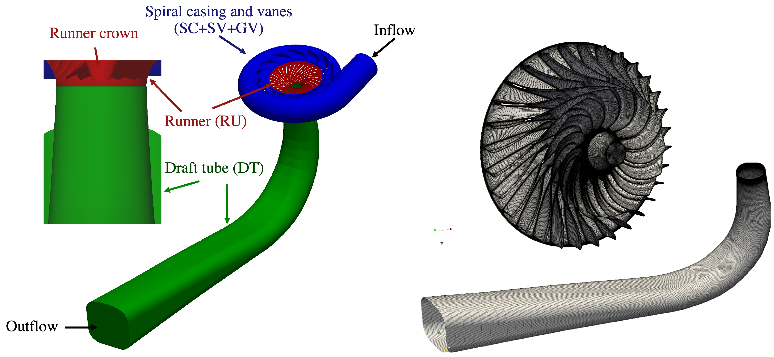
In this paper, the Francis-99 turbine model is used. This turbine is a scaled-down model of the prototype Francis turbine installed at the Tokke power plant in Norway [34]. The computational domain shown in Figure 1 includes the spiral casing, the stay vanes, the guide vanes, the runner, and the draft tube. There are 14 stay vanes and 28 guide vanes. The runner includes 15 splitter blades and 15 full-length blades. The inlet and outlet diameters of the runner are 0.63 m and 0.347 m, respectively. The mesh in different components of the turbine are produced using the Pointwise V18.3 mesh generation software. The mesh specifications for each component are shown in Table 1. The mesh has 20.88 M cells, which according to the mesh dependency studies performed for simulations of the Francis-99 turbine found in the literature [35,36,37,38,39] is enough for mesh-independent results of the flow in the draft tube. The table also shows that the average value is larger than 1 for all components; therefore, the wall function based on Spalding’s law is used at the walls [25,40,41]. It should be mentioned that using the wall function for the simulations of the flow in the draft tube of Francis turbines is justified as the work by Wilhelm et al. [42] showed that resolving near-wall regions instead of using the wall function has insignificant effects on the captured flow in the draft tube.
As mentioned in Section 2, we use a zonal WMLES approach where the RANS and WMLES approaches are used in different regions of the domain. Since the focus of the paper is to investigate the RVR in the draft tube, we use the WMLES approach in the draft tube (region labeled by DT in Figure 1) and in the rest of the domain (regions labeled by RU, SC, SV, and GV in Figure 1), the RANS approach is employed.
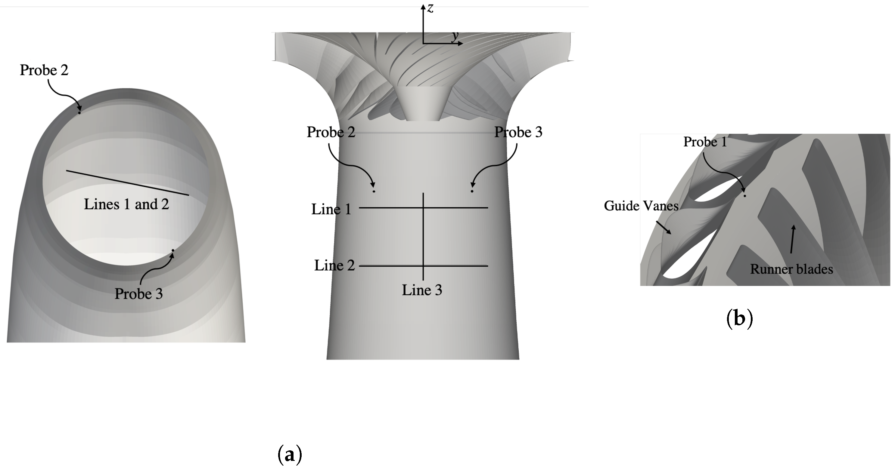
The experimental data used for validation in the present study are from the second Francis-99 workshop. These data include both pressure and velocity measurements at different locations. The velocity measurements includes the axial and horizontal components over three lines in the draft tube, Line 1, Line 2, and Line 3 in Figure 2a. The data also include the static pressure fluctuations at two probes in the draft tube, Probe 2 and Probe 3 in Figure 2a and the static pressure in the vaneless region between the guide vane blades and runner blades, is marked by Probe 1 in Figure 2b.
3.1. Studied Flow Conditions
In this paper, the part-load (PL) condition in the second Francis-99 workshop is studied. In this condition, the guide vane opening is , the runner angular speed is , and the discharge is . In order to study the effect of cavitation in this PL condition, the simulations are performed for both non-cavitating and cavitating conditions. The cavitation number, , in these simulations is defined as
where and are, respectively, the pressure and the cross-section area at the draft tube outlet, is the vapour pressure, is liquid density, and H is the turbine head. Here, we study the flows at which includes the near-inception cavitation in the RVR () as well as the condition corresponding to the fully cavitating RVR ().
4. Results
The results are divided into two parts. The first part presents the effect of turbulence modeling on capturing the global quantities, the velocity profiles and the pressure fluctuations in the draft tube. The second part is devoted to studying the effects of cavitation on the same flow features.
4.1. Effect of Turbulence Modeling
In Table 2, the global quantities captured with different turbulence modeling techniques are compared with the experimental values. The relative errors in this table are obtained by dividing the difference between the experimental and numerical values by the experimental values. This comparison shows that all of the turbulence modeling techniques can capture these global quantities with a relatively small error, although a slightly lower relative error can be seen in the WMLES results. According to Čelič and Ondráčka [43], this error can be due to neglecting the labyrinth seal and disk friction losses.
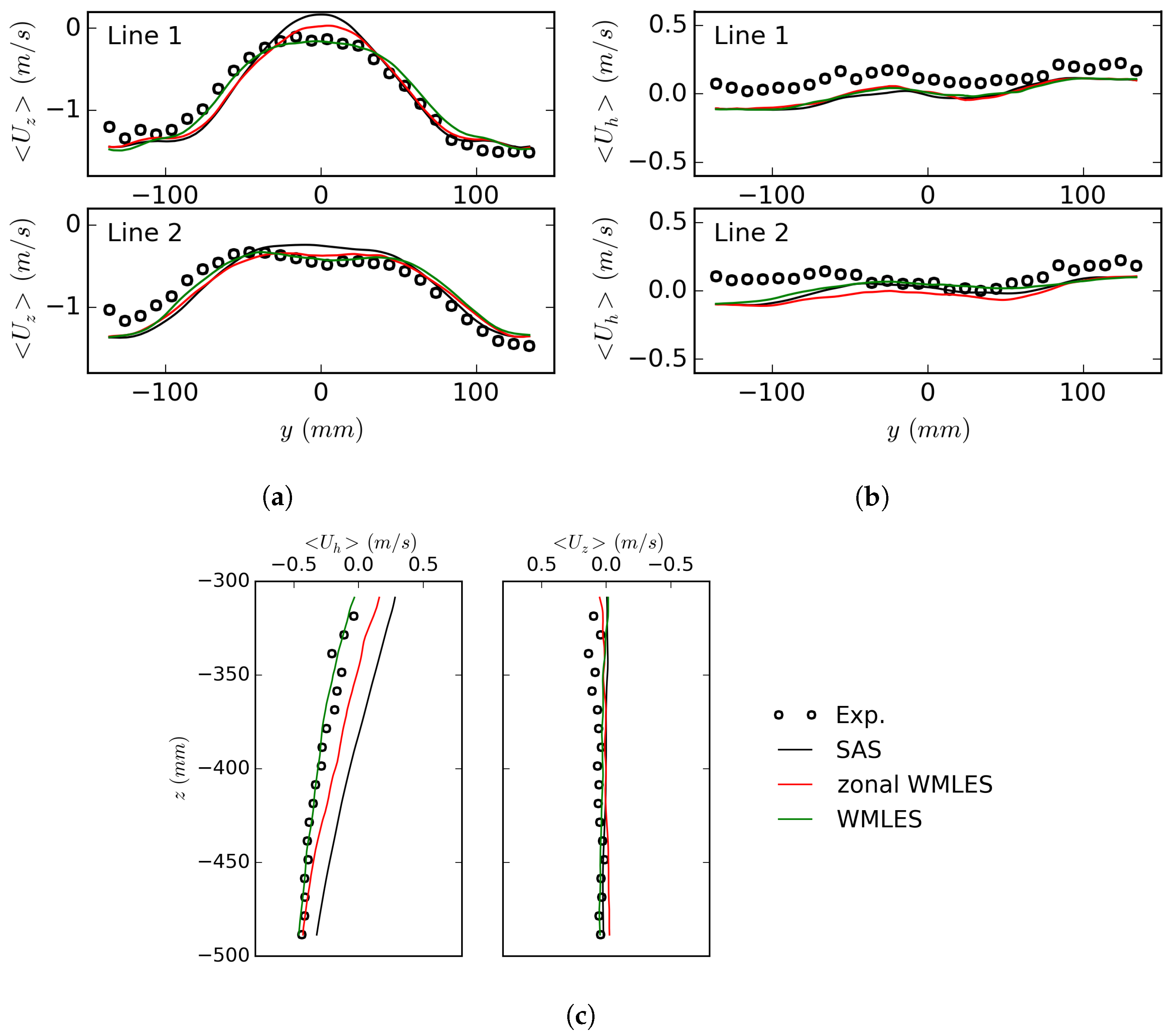
Figure 3 compares the time-averaged experimental and numerical velocity profiles along the three lines shown in Figure 2a. The experimental profiles are taken from the data provided by the second Francis-99 workshop [44]. The experimental axial velocity over Line 1 and Line 2 indicates that a region with low values of absolute axial velocity exists near the center of the draft tube. The comparison between the numerical results in Figure 3a,c indicates that this region is captured by all simulations, although there are some quantitative differences between the different results. As it can be seen in the axial velocity profiles on Lines 1 and 2 (Figure 3a), the regions with low values of absolute axial velocity in the SAS and zonal WMLES results are more confined to the center of the draft tube cone compared to the WMLES results and the experimental data. The axial velocity along the centerline (Figure 3c) shows that while the WMLES simulation predicts a negative averaged axial velocity along the entire Line 3, similar to the experimental data, positive values for the time-averaged axial velocity can be seen in the SAS and zonal WMLES results. Considering the definition of the axial direction (z), shown in Figure 2a, this positive axial velocity means that there is a reversed flow along the centerline of the draft tube cone in these two simulations. The cause of this difference is explained later in this paper. The horizontal velocity profiles (Figure 3b,c) show that the simulations can capture the trends similar to the experiment. However, the values of horizontal velocity in these simulations are shifted compared with the experimental values. It should be noted that the absolute value of the horizontal velocity is very close to zero over the measurement lines, the relative uncertainty for these velocities is higher compared with that for the axial velocities according to Salehi and Nilsson [45]. This higher uncertainty can be one reason for the difference between the results for these velocity profiles.
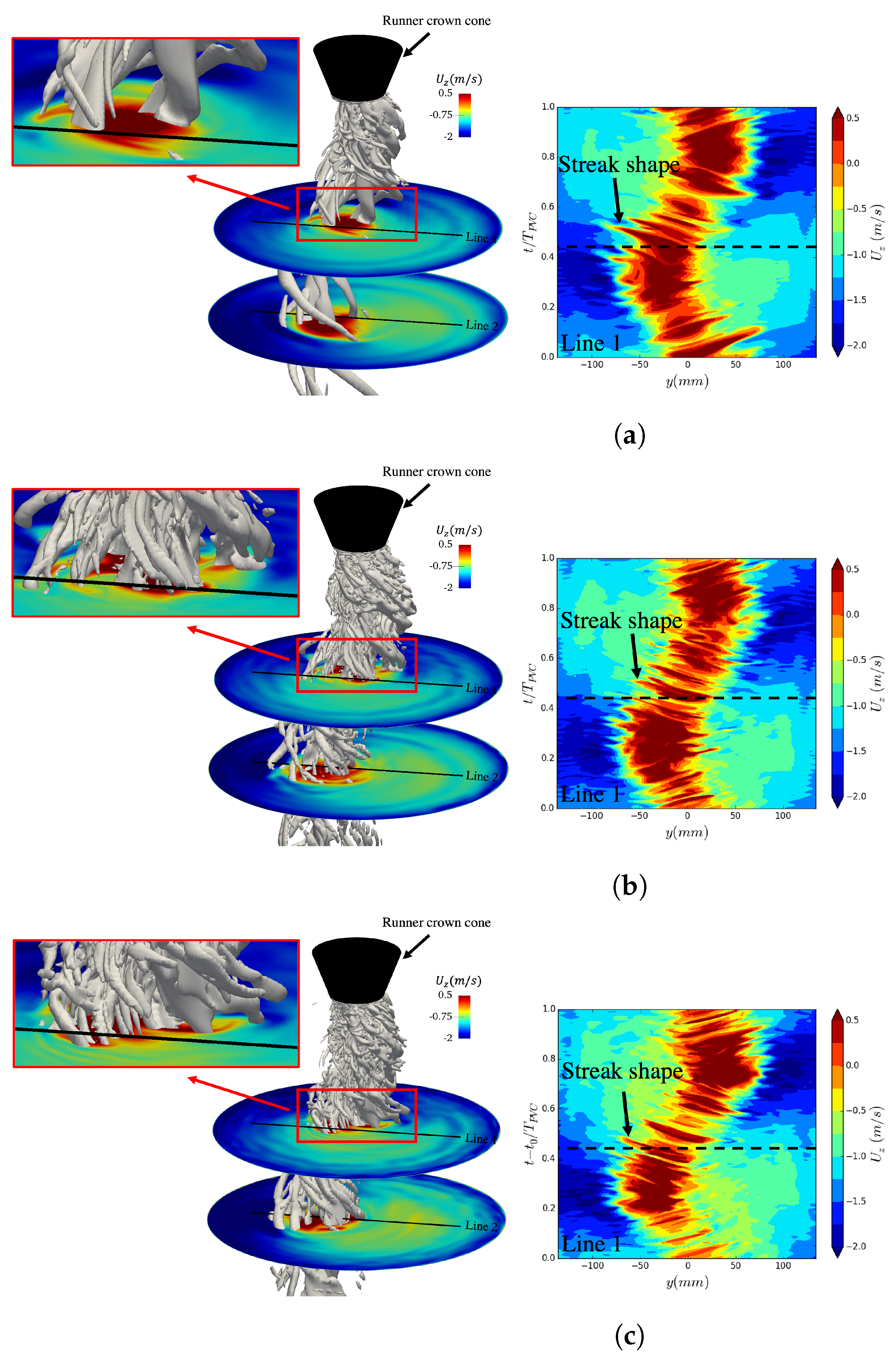
It is well-established that the region with low values of absolute axial velocity shown in Figure 3 is caused by the formation of the RVR in the draft tube at part-load condition. Figure 4 shows snapshots of the RVRs of the different numerical results. In this figure, the RVRs are visualized using an iso-surface of Q, which is the second invariant of the velocity gradient tensor. The level of the iso-surface is , which is chosen for an optimal visualization of the RVRs. In the zoom-in view, it can be seen that the RVR consists of many vortices wrapping around each other. At the location of these vorticies, the positive value of axial velocity (red color in the figure) indicates the presence of a reversed flow. The figure also presents the time history of the axial velocity on Line 1 for one period of the RVR rotation. The time instance corresponding to the snapshot of the iso-surfaces is shown by black dashed lines. These time histories show that as the RVR passes Line 1, the axial velocity on these lines becomes positive (red regions). The sweeping motion of the vortices causes the tilted streaks seen in the time history. A comparison between the results from the different simulations indicates that the number and size of the vortices in the RVR are strongly influenced by the selection of the turbulence modeling technique. In the SAS simulation, the RVR consists of a small number of large vortices, as shown in the zoom-in views, and this leads to fewer and large streaks in the time history of the axial velocity. In the zonal WMLES and WMLES simulations, however, the RVR has a large number of smaller vortices, which creates thinner streaks in the time history.
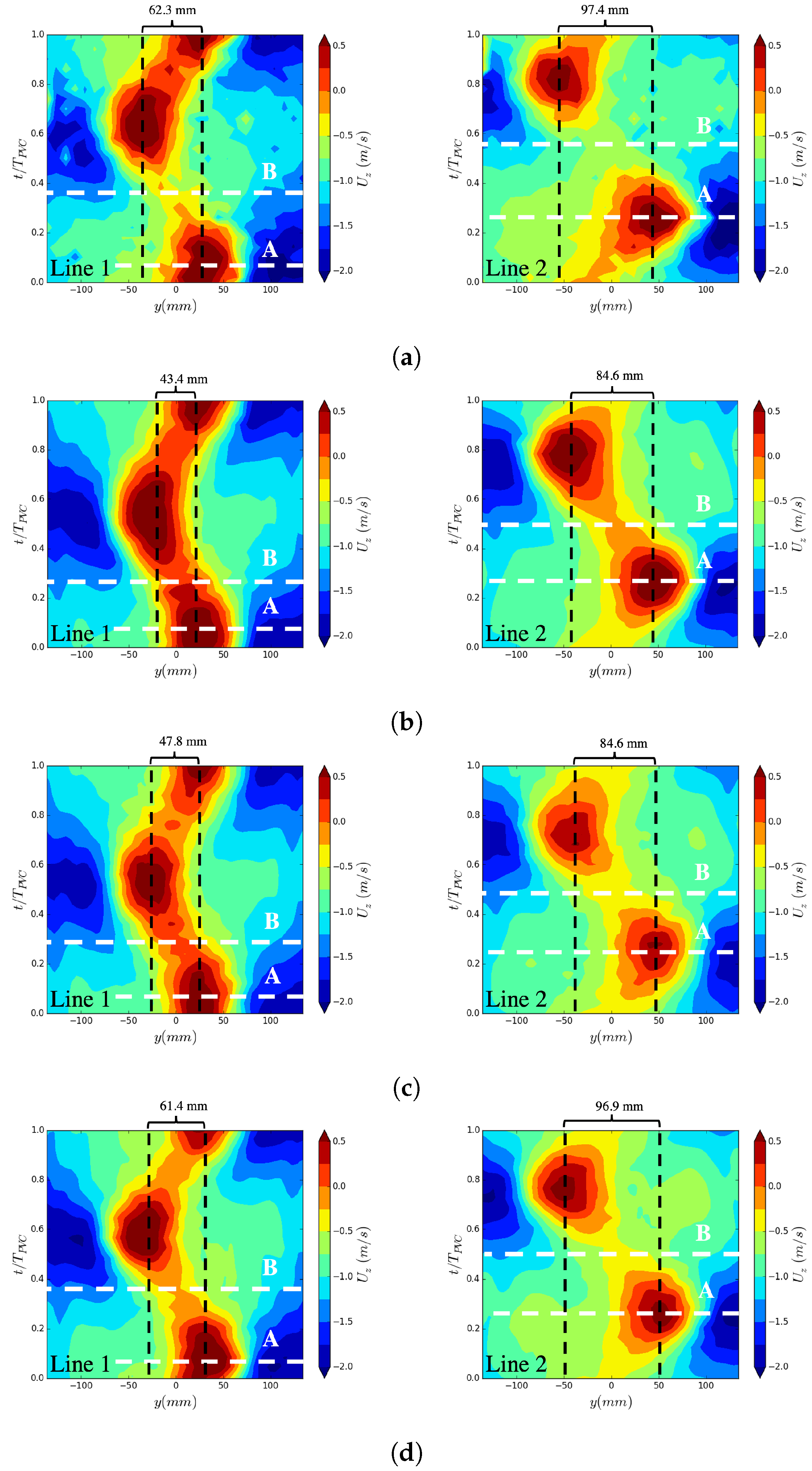
As mentioned earlier and shown in Figure 3, the region with a low value of absolute axial velocity in the center of the draft tube cone is affected by the selection of the turbulence modeling. To provide a reason for this effect, the phase-averaged axial velocity over Lines 1 and 2 in the experiment and simulations is shown in Figure 5. To obtain the phase-averaged values in this paper, the data signal corresponding to one cycle of the RVR rotation, , is divided into 30 windows. The data corresponding to each window are averaged together. Two instances A and B are marked in these figures. At instance A, the axial velocity has a high positive value which is due to the passage of the RVR over the measurement lines. At instance B, the RVR has rotated further and left the measurement lines, which leads to the observed decrease in the axial velocity toward the negative values. The comparison in Figure 5 shows that when the vortex passes the measurement lines at instance A, all simulations predict a distribution of axial velocity which is quite similar to the experimental data. However, this is not case for the instance when the RVR leaves the measurement lines (instance B). At this instance, the axial velocity over Line 1 near the center of the draft tube ( mm) has positive values in the SAS and zonal WMLES simulations while the values in the experiment and the WMLES simulations are negative. The reason for this difference is that the RVR in the SAS and zonal WMLES simulations rotates on a path which is closer to the center of draft tube as compared with the experiment and the WMLES simulation. To clearly show this, the figure shows vertical black lines passing through the maximum values of axial velocity when the RVR is on the measurement line. The distance between these lines is also shown. It can be seen that distance between these lines is larger in the experiment and the WMLES results as compared with the other two simulations. This difference means that a portion of the RVR in the SAS and zonal WMLES simulations has overlaps with Line 1 near the center of the draft tube all through the rotational cycle of the RVR. Since the axial velocity in the RVR is positive according to Figure 4, this overlap would lead to the positive values of axial velocity over Line 1 at instance B in the SAS and zonal WMLES simulations. It also leads to the positive values of the averaged axial velocity in these two simulations which is shown in Figure 3.
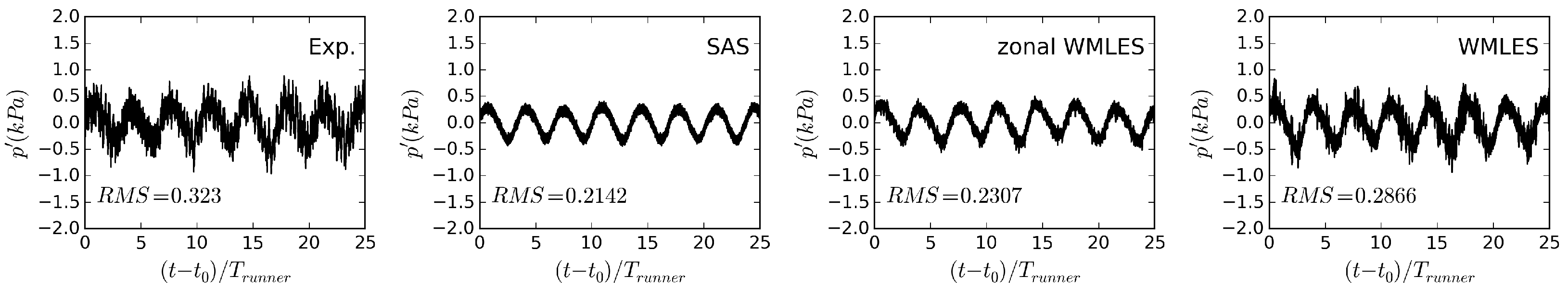
The RVR in the draft tube creates a large amount of pressure fluctuations which can lead to vibrations. To evaluate how well these pressure fluctuations can be captured by the different turbulence modeling techniques, Figure 6 compares the experimental and numerical pressure fluctuation signals in Probe 2 in the draft tube. For each signal, the Root Mean Square (RMS) of the fluctuations is noted in the plot. It can be seen that in all of the numerical results, the RMS values are lower compared with the values in the experiment. The numerical RMS values however increase towards the experimental one as the resolution of the turbulence modeling technique increases. It can be seen that, as expected, it is mainly the smaller scales of the fluctuations that differ between the results from the different turbulence modeling techniques, while the amplitude and frequency of the large-scale RVR motion are similar.
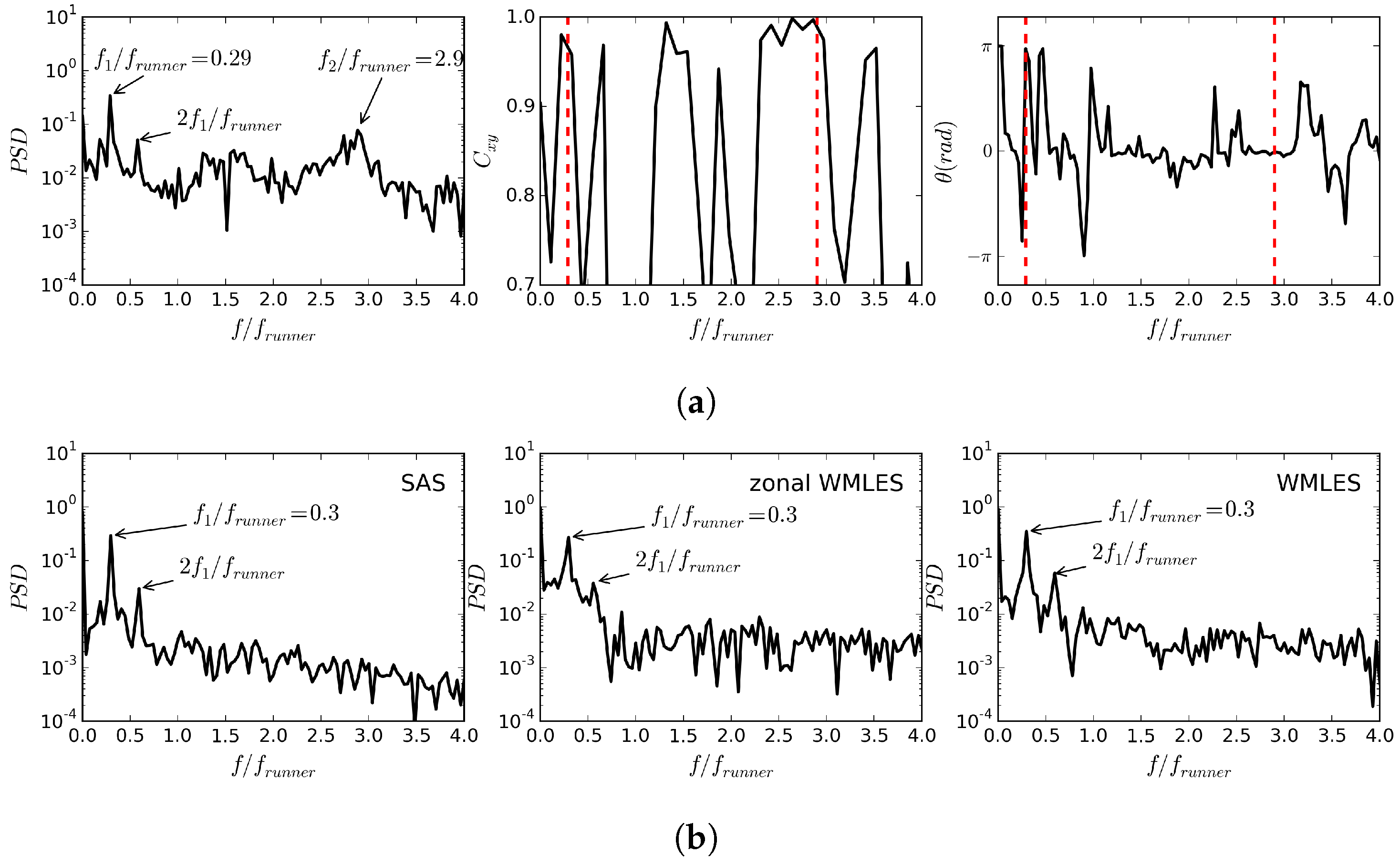
To investigate the reasons why the RMS values of the pressure fluctuations are lower in the simulations compared with the experiment, Figure 7 shows a frequency analysis of the pressure fluctuations. For the experiment, the analysis (Figure 7a) includes the power spectrum analysis of the pressure signal from Probe 2 (left plot), the coherence (middle plot), and the phase difference (right plot) between the pressure signals from Probes 2 and 3. The coherence and phase difference between the two signals are calculated from the cross-spectral density, , which is obtained using Welch’s method [46]. The frequency analysis of the experimental pressure signal (left plot) indicates the existence of two dominant frequencies, and . For these dominant frequencies, the coherence between the signals at Probes 2 and 3 (middle plot) is almost one, which means that these dominant frequencies also exist in the signal from Probe 3. The phase difference between the two signals (right plot) is for the dominant frequency and its harmonic . Considering that the locations of Probes 2 and 3 are exactly at opposite sides of the cone region in the draft tube, this phase difference suggests that the dominant frequency, , is due to the precession of the RVR in the draft tube cone. It should be mentioned that the precession frequency is in the range 0.2–0.4 , which has been found in previous studies [7,47]. For the dominant frequency , the phase difference is almost zero indicating that the corresponding pressure fluctuations are synchronous meaning that they have the same phase and amplitude for the pressure sensors located in the same cross section of the draft tube. The frequency analyses of the pressure signals in the simulations with different turbulence modeling techniques show that the dominant frequency of the RVR, , and its harmonic, , is captured by all turbulence modeling techniques. The experimental dominant frequency can however not be seen in any of the numerical results, which causes a reduced RMS value.
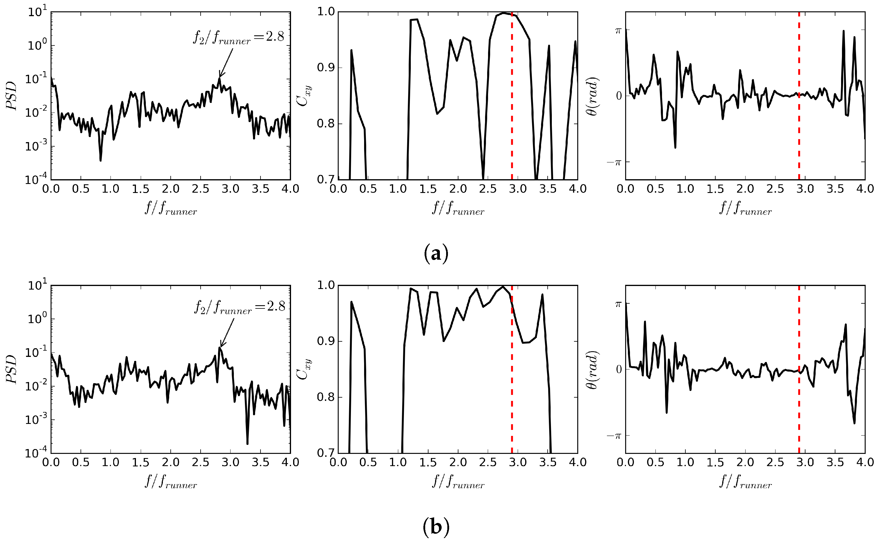
To investigate the origin of the dominant frequency in the experiment, Figure 8 shows a spectral analysis of the pressure fluctuations in the draft tube at the Best Efficiency Point (BEP) and High Load (HL) conditions for which there is no RVR. Similar to the PL condition, a dominant frequency at can be seen also for BEP and HL (left plots). As for the PL condition, the coherence (middle plots) is close to one and the phase difference (right plots) is zero for this frequency. This indicates a synchronous nature of these pressure fluctuations, at a frequency that is rather independent of the operating condition. Based on this observation, we can conclude that the synchronous pressure fluctuations seen in the experimental results is related to a component in the system rather than the flow features in the components studied here. It should be mentioned that similar synchronous pressure fluctuations have been observed by Favrel et al. [8], Arpe et al. [9], with frequencies in the range of 2–4 . These studies, however, have shown that this type of pressure fluctuations occurs in cavitating conditions and can be attributed to the interaction between the cavitating RVR and the elbow in the draft tube.
To further analyze the high-frequency content of the signals and its effects on the RMS values, the fluctuations are decomposed into two components as
where denotes the pressure fluctuations due to the precession of the RVR and denotes the pressure fluctuations due to other sources. To perform this decomposition, we assume that the pressure fluctuations due to RVR at Probe 2 have a phase difference of with the corresponding fluctuations at Probe 3. This assumption is shown to be true in Figure 7a. Based on this assumption, the frequencies of pressure fluctuations due to RVR are determined. These frequencies are then filtered from the signal of pressure fluctuations to obtain the pressure fluctuations due to other sources, . The fluctuations due to RVR, , then can be obtained by subtracting from the original pressure fluctuation signal according to Equation (22).
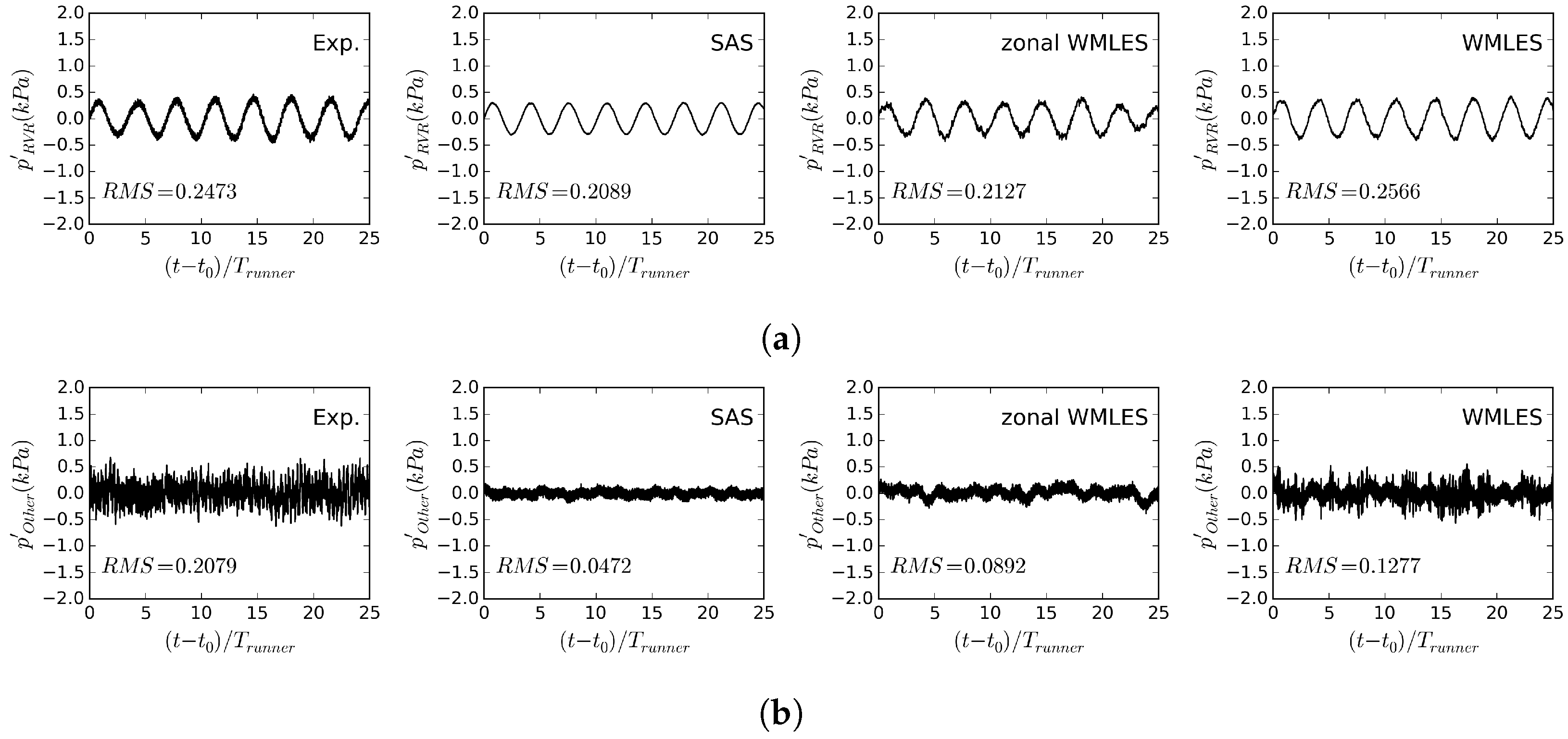
Figure 9 shows the different components of the pressure fluctuations at Probe 2 according to Equation (22) and their corresponding RMS values from the results of the simulations and experiment. For the pressure fluctuations due to the RVR, the difference between the predicted RMS values and the experimental RMS value correspond to 16%, 14% and 4% for the SAS, zonal WMLES and WMLES simulations, respectively. The reason for these differences will be explained later. The corresponding differences for the pressure fluctuations due to other sources are 77%, 59%, and 39%. The reason for these large differences is mainly that (as shown before) the numerical fluctuations do not include the synchronous pressure fluctuations with the experimental dominant frequency of shown in Figure 7a. The comparison between the results of the different simulations also shows that the RMS values of are very sensitive to the selected turbulence modeling technique. This type of pressure fluctuations includes the pressure fluctuations due to wakes of the guide vanes, runner blades, and runner crown which are captured to a larger extent in the WMLES simulation compared with the zonal WMLES and SAS simulations, for which the region upstream the draft tube is resolved using a RANS approach.
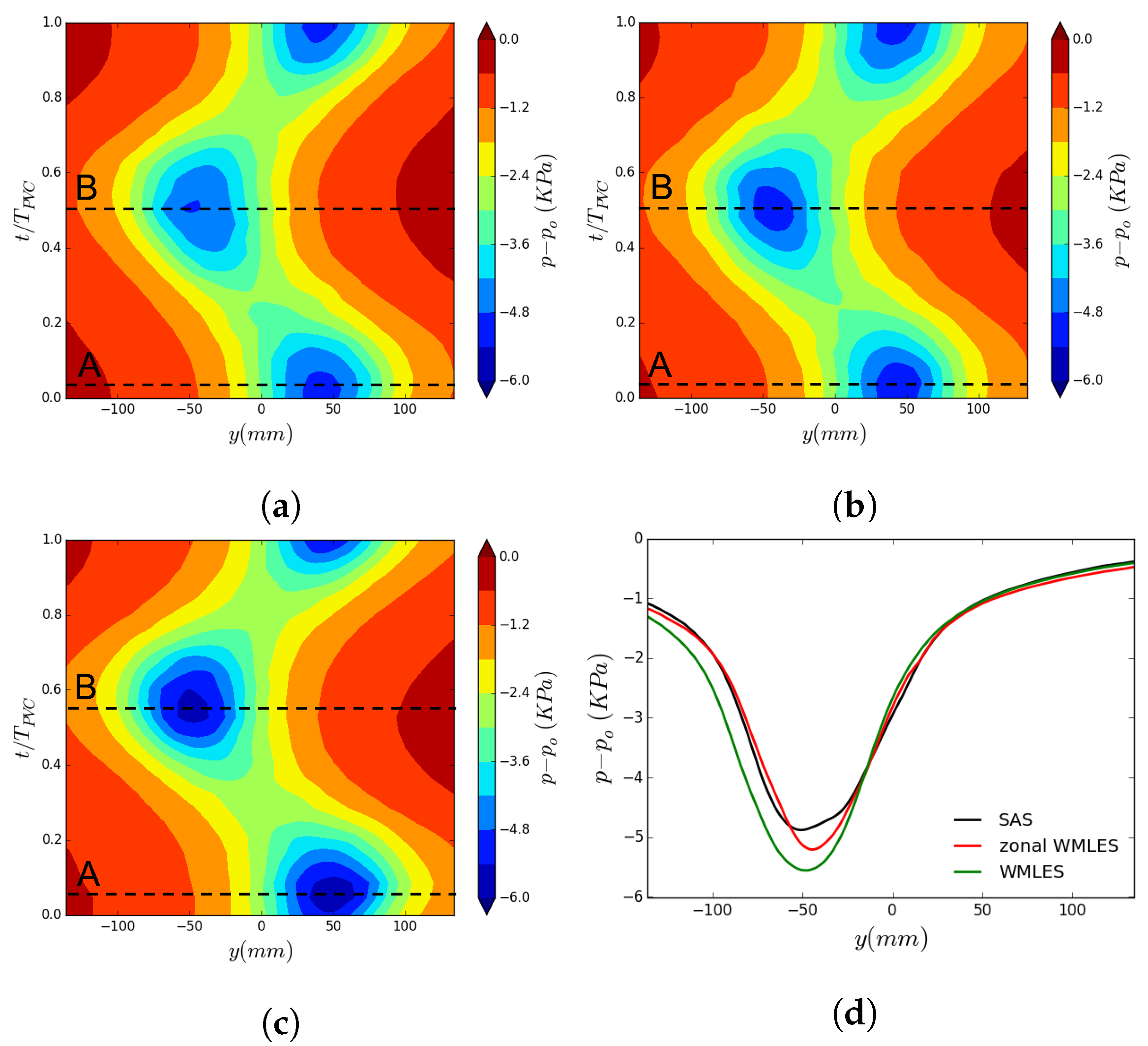
The comparison between the RMS values of the pressure fluctuations due to the RVR in Figure 9a showed that the predicted value from the WMLES simulation is closer to the experimental value than the values using the other turbulence modeling techniques. In order to investigate the reason for this and also study the effect of turbulence modeling on the pressure field in the draft tube, Figure 10 shows the phase-averaged pressure over Line 1 with the different turbulence modeling techniques. The core of the RVR, where the pressure is low, passes Line 1 at instances A and B. It can be seen that the RVR core pressure drops more in the WMLES results compared with the results of the other turbulence modeling techniques. A more quantitative comparison is shown in Figure 10d, at time instance B only. It can be seen that the pressure field far from the vortex core ( mm) is almost the same in all simulations. However, the pressure in the near-field of the RVR ( mm) is affected by the choice of turbulence modeling technique. In the WMLES results, the minimum pressure in the near-field is lower and the extent of the low pressure region is larger and slightly closer to the nearest wall compared with the other two results. This can explain the higher RMS level of the pressure fluctuations due to the RVR in the WMLES simulation as shown in Figure 9a. It should particularly be stressed that capturing the correct pressure drop in the RVR is very important for cavitating simulations as this pressure drop is the driving force of the cavitation formation. In WMLES simulations, where a larger pressure drop can be captured, a larger volume of cavitation should be expected in cavitating simulations.
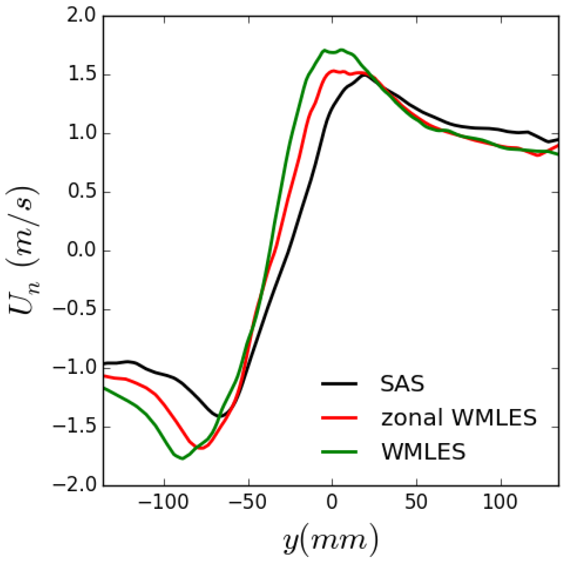
To explain the reason for the larger pressure drop in the RVR of the WMLES simulation, Figure 11 shows the phase-averaged normal velocity over Line 1 at time instance B that was shown in Figure 10. The center of the RVR approximately corresponds to due to the rotating flow around the center of the RVR. The comparison between the numerical results shows that the gradient of the normal velocity is larger around the center of the RVR in the WMLES result than with the other turbulence model techniques. This indicates that the swirling motion around the RVR in the WMLES simulation is stronger, which leads to the larger pressure drop shown in Figure 10.
4.2. Effect of Cavitation
As mentioned in Section 3.1, cavitation simulations using WMLES are performed for three different cavitation numbers to study the effect of cavitation on the global quantities, the velocity profiles and the pressure fluctuations in the draft tube. It should be mentioned that since there are no experimental data for cavitating conditions in a Francis-99 turbine, no comparison is made between the simulation results and experimental ones. To show the extent of the cavitating region in these simulations, Figure 12 presents the cavitating part of the RVR using a blue iso-surface of . This figure also shows the variation of the total volume of vapor in the RVR as well as a spectral analysis of this variation. It can be seen that the cavitation inception at happens at the root of the RVR near the runner crown. The total vapor content at this condition exhibits significant fluctuations, indicating that the cavitation is highly unstable. The spectral analysis of the vapor volume variation shows that this instability in the cavity volume does not have any dominant frequency. By decreasing the cavitation number to , the cavitation starts to incept in the small vortices further downstream the runner exit. Similar to the previous condition, the cavitation is unstable, although with a lower frequency. The spectral analysis indicates that although there is an increase in the PSD level of frequencies lower than , this increase does not lead to a dominant peak in the PSD level. By further decreasing the cavitation number to , the cavitating region covers almost the entire root of the RVR near the runner exit. The variation of vapor volume indicates that there are fluctuations in the size of the cavitating region of the vortex. Unlike the other two cavitating conditions, the spectral analysis shows that these fluctuations have a dominant frequency at .
Table 3 presents the global quantities in the form of torque, , head, H, and efficiency , for the different cavitation numbers and for the non-cavitating condition (). It can be seen that the cavitation number does not have any significant effect on these quantities, as the maximum variation in these quantities with respect to the cavitation number is less than 0.2 percent. This is expected, as the studied cavitation numbers are far from the cavitation breakdown for the studied turbine [48].
To study the effect of cavitation on the velocity field, Figure 13 shows the time-averaged velocity profiles on Lines 1–3 (shown in Figure 2) for different cavitation numbers. It can be seen that cavitation does not have any effect on these velocity profiles for and . For these conditions, the size of the region with low values of absolute axial velocity is almost identical to the size of this region in the non-cavitating condition. In the fully cavitating RVR in the simulation with , however, the velocity profiles are slightly affected by the presence of cavitation. This effect is more dominant in the profiles for Line 1 as this line is closer to the cavitating part of the RVR.
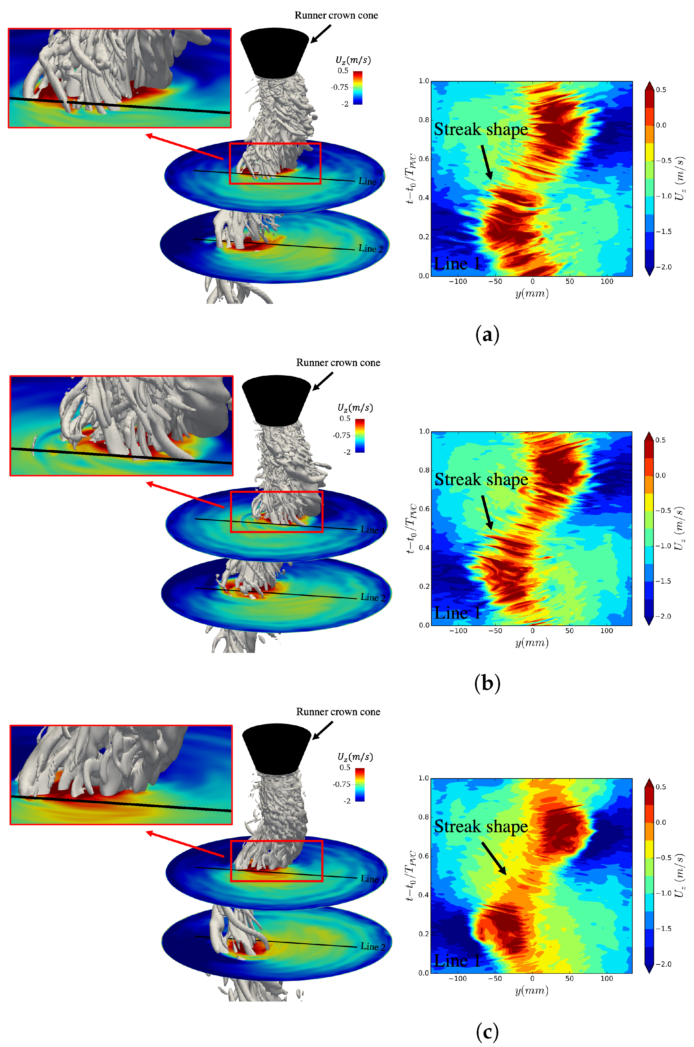
In order to investigate the effects of cavitation on the structure of the RVR and the instantaneous velocity field, Figure 14 presents the iso-surface of the Q criterion (left plots) and the history of the axial velocity over Line 1 for one period of vortex rotation (right plots) for different cavitation numbers. The iso-surface of the Q-criterion shows that similar to the non-cavitating condition, shown in Figure 4c, the RVR of the cavitating conditions consists of small vortices and there is a reverse flow at the location of these small vortices. The plots of history of the axial velocity on Line 1 show that streaks are formed as these vorticies and their reverse flows pass Line 1. A comparison between the results for the different cavitation numbers shows that the reversed flow in these streaks is highly affected by the presence of cavitation. At , for which the amount of cavitation in the RVR is small, the reverse flow in the streaks is quite similar to the non-cavitating condition (see Figure 4c). As the amount of cavitation increases, for and , the reverse flow in the streaks becomes weaker.
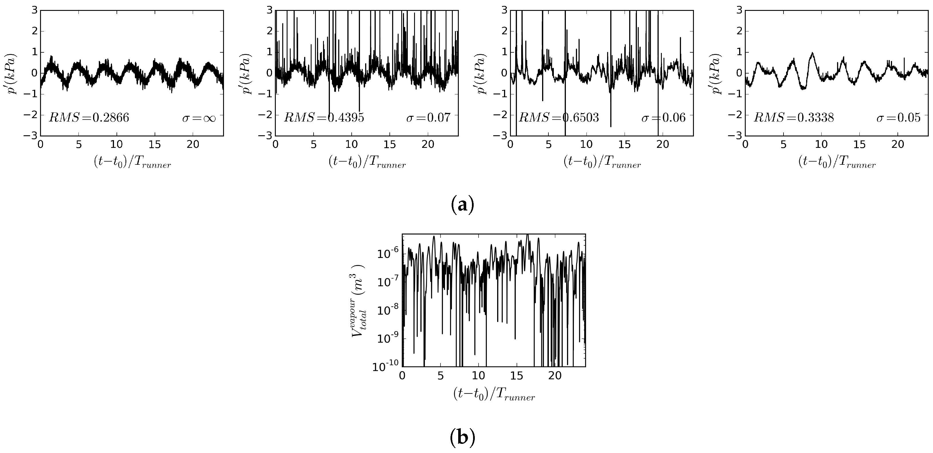
Figure 15a shows the pressure fluctuations at Probe 2 for different cavitation numbers, including their RMS values. It can be seen that the inception of cavitation (at ) leads to spikes in the pressure fluctuations, which is due to the collapse of the cavitation region. This can be seen in Figure 15b, where the total vapor volume decreases to near-zero values at the time of the pressure spikes. Due to these spikes, the RMS of the pressure fluctuations increases by 54% compared to the non-cavitating case. It should be noted that the spikes are truncated in the plot in order to keep a scale that still shows the variations due to the RVR. By slightly increasing the amount of cavitation (for ), the spikes are not as frequent as those at , which indicates that the cavitation region is less frequently entirely collapsing. This is confirmed in Figure 12b, where the total volume fraction goes to zero less frequently than in Figure 12a. There is however a further increase in the RMS value as the cavitation number is decreased from to , indicating that the collapses of the larger cavitation regions give higher pressure pulses. Again, it should be noted that the spikes are truncated in the plot. In the case of the fully cavitating RVR, at , most of the spikes are gone. This indicates that the cavitation region never collapses entirely (confirmed in Figure 12c), and that the collapses of smaller cavitation regions in the freestream give much smaller pressure spikes. This leads to smaller RMS values. On the other hand, it can clearly be seen that the variations due to the RVR is much less periodic at than for the other cavitation numbers, indicating that the general flow features are influenced to a larger extent. In accordance with the increase in the RMS value compared to the non-cavitating condition, the cavitation increases the amplitude of the variations due to the RVR as a major contributor to the RMS value.
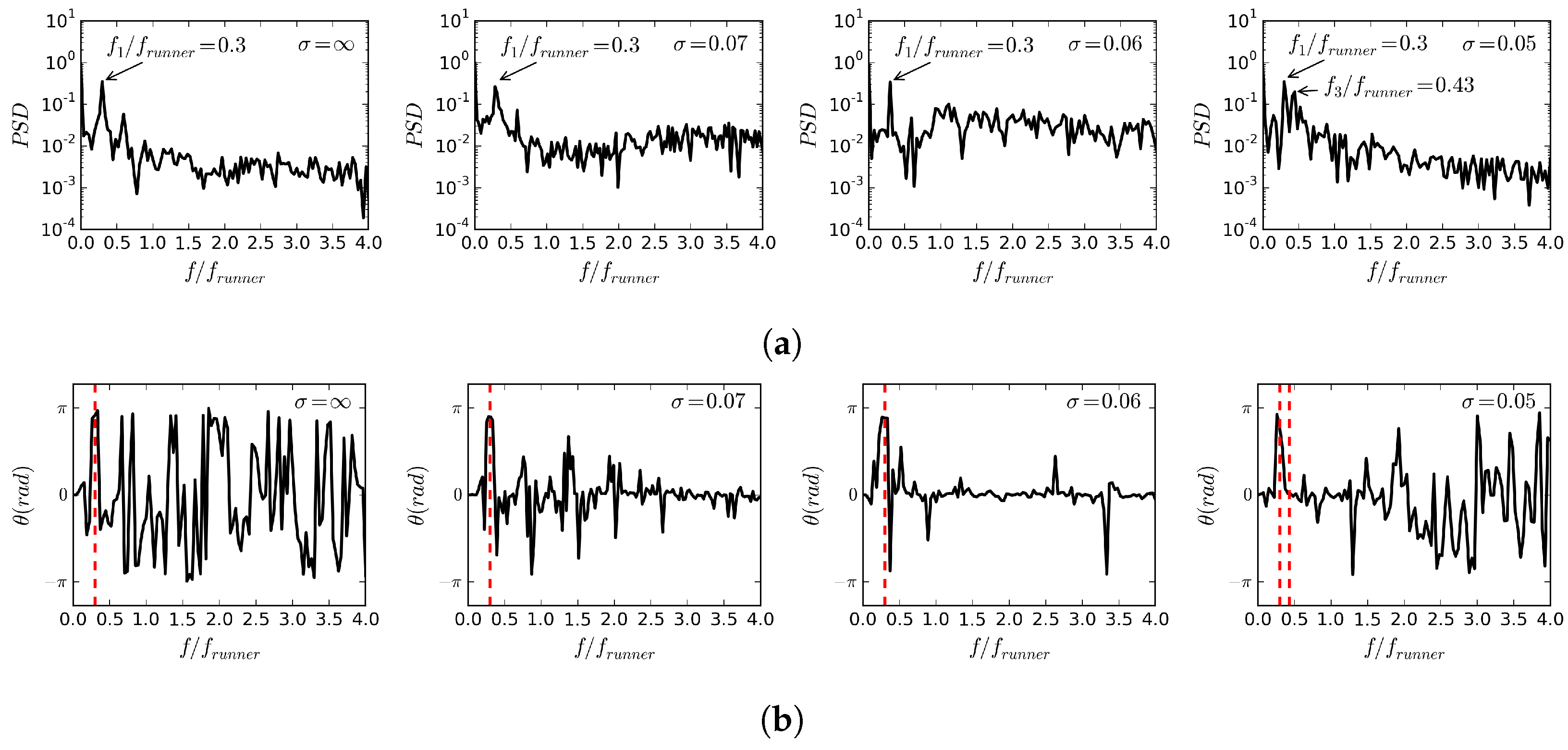
Figure 16 shows spectral analyses of the pressure fluctuations at Probe 2 for the different cavitation numbers, as well as the phase difference between the pressure fluctuations at Probes 2 and 3. The spectral analyses show that the dominant frequency, , is not affected by the presence of cavitation. As mentioned earlier, this frequency is related to the frequency of the RVR rotation. A comparison between the non-cavitating and cavitating conditions indicates that cavitation mostly affects the PSD level of the higher frequencies rather than that of the relatively low RVR frequency. For , at cavitation inception, an increase can be seen in the PSD level of frequencies larger than . By further increasing the amount of cavitation, at , the increase in the PSD level of the pressure fluctuations happens already at . At , the increase in the PSD level approaches the frequency, with a local peak at , and the PSD level of the higher frequencies again decreases. The frequency of the additional peak is the same as the dominant frequency of the vapor volume fluctuations for this cavitation number, as shown in Figure 12c. The phase difference between the pressure fluctuations at Probes 2 and 3, shown in Figure 16b, shows that for the frequencies where there is an increase in the PSD level due to cavitation, the phase difference is highly reduced (approaching zero). This means that the increased pressure fluctuations in these frequencies are synchronous.
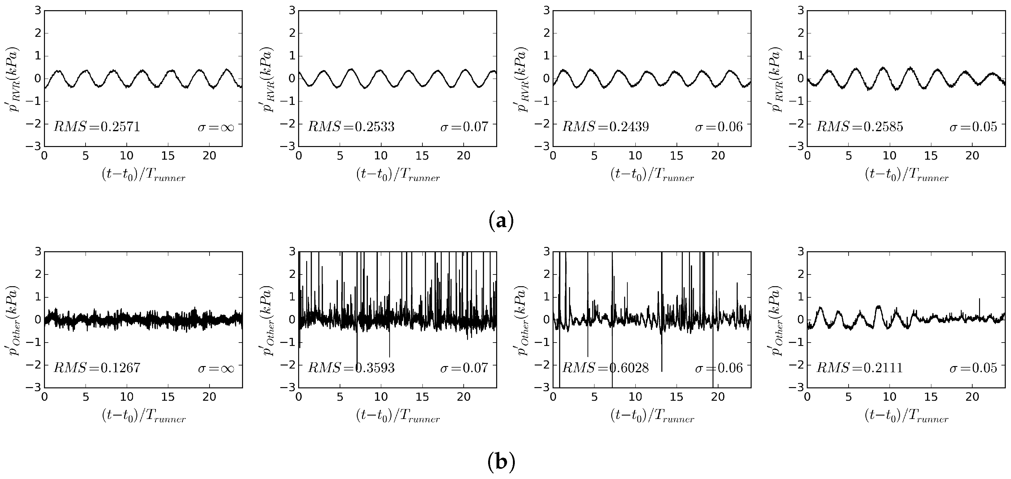
Figure 17 shows the effects of cavitation on the different components of the pressure fluctuations and their RMS values, decomposed according to Equation (22). It can be seen that the cavitation has insignificant effects on the RMS values of the pressure fluctuations due to the RVR, as the maximum difference between the RMS values for the different cavitation numbers is around 7%. However, the RMS values of the other sources are highly affected by the presence of cavitation. Similar to the trends shown in Figure 15a, the RMS of the synchronous pressure fluctuations first increases as the amount of cavitation increases ( and ), and then decreases when the RVR is fully cavitating ().
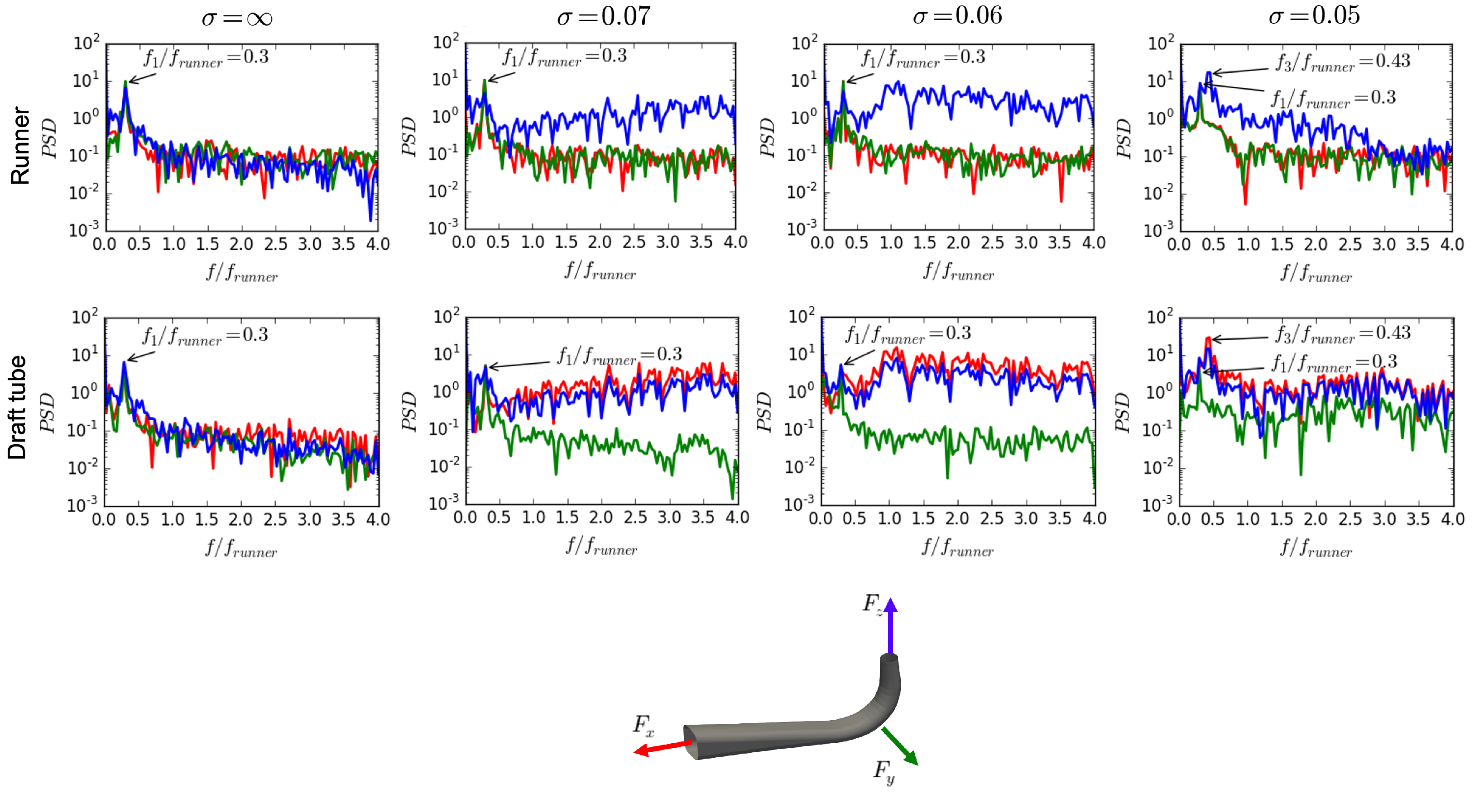
Figure 18 shows the effects of cavitation on the forces exerted on the runner and draft tube in the frequency domain. For the runner, only the z-component of the force (the blue curve) is affected by the cavitation, while for the draft tube, both the x- and z-components of the forces (red and blue curves, respectively) are affected by the cavitation. The trends of the changes due to cavitation, however, are the same for these affected force components, and they are quite similar to the trends for the pressure fluctuations shown in Figure 16a. At , where the amount of cavitation is small, there is an increase in the PSD level of the high-frequency fluctuations of the affected force components. The same increase can be seen for , although the increase in the PSD level starts to appear already at lower frequencies. At , this increase in PSD level leads to the dominant frequency , which is the same as the dominant frequency of the vapor volume fluctuations as shown in Figure 12c. It should be mentioned that the changes in the forces discussed here are caused by cavitation-induced pressure fluctuations, which are shown to be synchronous in Figure 16. Due to the synchronous nature of these pressure fluctuations, they affect only the forces in the directions where the geometry is asymmetrical. In the symmetrical directions, the changes in the forces due to these pressure fluctuations cancel each other out. For the runner, the geometry is almost symmetrical with respect to the x- and y-directions, and therefore, the cavitation-induced pressure fluctuations can affect only the forces in the z-direction. In the draft tube, however, the geometry is symmetric only with respect to the y-direction, and the effects of cavitation can be seen both in the x- and z-components of the forces.
5. Conclusions
In this work, we examine non-cavitating and cavitating RVR (Rotating Vortex Rope) in the Francis-99 turbine model using scale-resolving approaches. The non-cavitating simulations are performed using the SST-SAS, zonal wall-modeled LES and wall-modeled LES (WM) approaches, and the results are compared with the experimental data made available by the Francis-99 workshop. Furthermore, cavitating simulations are conducted for three cavitation numbers using the WMLES approach. The results from these simulations are used to study the effects of cavitation on the flow features, such as the velocity distribution and pressure fluctuations in the draft tube, and the forces acting on the draft tube and the runner.
The comparison between the results of the non-cavitating simulations and the experimental data reveals that the averaged velocity profiles and the pressure fluctuations predicted by the WMLES approach are in better agreement with the experimental data compared with the SST-SAS and zonal WMLES approaches. It is shown for the first time that the better velocity prediction is related to a correctly predicted rotating path of the RVR in the WMLES simulation. In the SST-SAS and zonal WMLES simulations, the RVR rotates on a path which is closer to the center of the draft tube as compared to the WMLES simulation and experiment. This yields an over-prediction of the influence of the RVR on the time-averaged velocity profile near the center of the draft tube. The comparison between the numerical results and the experimental data also shows that all methods under-predict the RMS values of the pressure fluctuations in the experiment, although the predicted RMS of the pressure fluctuations using the WMLES approach is closest to the experimental value. Using a detailed analysis of the pressure fluctuations in the simulations and experiment, the reason for the difference between the numerical and experimental values is shown to be related to a synchronous type of fluctuations only appearing in the experimental data, with a dominant frequency of around 2.8 times the frequency of the runner. An analysis of the pressure fluctuations in the experimental data shows that this synchronous pressure fluctuations can be seen also at the BEP and HL conditions, which suggests that these synchronous pressure fluctuations are created by a component in the system rather than the RVR. Such a finding has not been reported in the previous studies on the Francis-99 turbine. It is also shown that the WMLES simulation can capture a larger pressure drop in the center of the RVR compared to the other two approaches, which is shown to be due to the larger swirling velocity around the RVR in the WMLES simulation.
The results from the cavitating simulations reveal that cavitation slightly affects the average velocity profiles in the draft only if there is a large amount of cavitation in the RVR. They also show that the presence of cavitation damps out the instantaneous reverse flow in the small vortices in the RVR. The pressure fluctuations are also shown to be significantly affected by the presence of cavitation. Cavitation induces synchronous pressure fluctuations with a frequency larger than the frequency of the RVR. Capturing these synchronous pressure fluctuations in simulations has previously not been reported in the literature. When the amount of cavitation in the RVR is small, these fluctuations have a broadband high-frequency spectrum, while in the case of a fully cavitating RVR, they have a dominant frequency close to the dominant frequency of the RVR. The analysis of the forces reveals that the cavitation-induced pressure fluctuations have different effects on the forces exerted on the runner and draft tube. In the runner, the presence of cavitation induces significant force fluctuations only in the direction aligned with the rotational axis of the runner, while the force fluctuations in the draft tube are additionally affected in the direction of the bend. This finding can be used to design a method to detect cavitation in the turbine based on the direction of the vibrations in the draft tube and runner.
Author Contributions
Conceptualization, M.H.A., R.E.B. and H.N.; methodology, M.H.A.; validation, M.H.A.; Analysis, M.H.A.; investigation, M.H.A.; writing—original draft preparation, M.H.A.; writing—review and editing, R.E.B. and H.N.; supervision, R.E.B. and H.N.; project administration, R.E.B. and H.N.; funding acquisition, R.E.B. and H.N. All authors have read and agreed to the published version of the manuscript.
Funding
The work was funded by Chalmers Energy Area of Advance and was carried out as a part of the “Swedish Hydropower Centre - SVC”. SVC is established by the Swedish Energy Agency, EnergiForsk and Svenska Kraftnät together with Luleå University of Technology, The Royal Institute of Technology, Chalmers University of Technology, and Uppsala University. The computations were enabled by resources provided by the Swedish National Infrastructure for Computing (SNIC) at NSC and C3SE partially funded by the Swedish Research Council through grant agreement no. 2018e05973. The investigated test case is provided by NTNU, Norwegian University of Science and Technology, under the Francis-99 workshop series.
Data Availability Statement
The data that support the findings of this study can be available from the corresponding author upon reasonable request.
Conflicts of Interest
The authors declare no conflict of interest.
References
- Rheingans, W. Power swings in hydroelectric powerplants. Trans. ASME 1940, 62, 171–184. [Google Scholar]
- Valentín, D.; Presas, A.; Egusquiza, E.; Valero, C.; Egusquiza, M.; Bossio, M. Power swing generated in Francis turbines by part load and overload instabilities. Energies 2017, 10, 2124. [Google Scholar] [CrossRef]
- Arndt, R.E.; Voigt, R.L., Jr.; Sinclair, J.P.; Rodrique, P.; Ferreira, A. Cavitation erosion in hydroturbines. J. Hydraul. Eng. 1989, 115, 1297–1315. [Google Scholar] [CrossRef]
- Avellan, F. Introduction to Cavitation in Hydraulic Machinery; Technical Report; Politehnica University of Timișoara: Timișoara, Romania, 2004. [Google Scholar]
- Brennen, C. Cavitation and Bubble Dynamics; Cambridge University Press: Cambridge, UK, 2014. [Google Scholar]
- Nishi, M.; Kubota, T.; Matsunaga, S.; Senoo, Y. Study on swirl flow and surge in an elbow type draft tube. In Proceedings of the 10th IAHR Symposium on Hydraulic Machinery and Cavitation, Tokyo, Japan, 28 September–2 October 1980; Volume 1, pp. 557–568. [Google Scholar]
- Iliescu, M.; Ciocan, G.; Avellan, F. Analysis of the cavitating draft tube vortex in a Francis turbine using particle image velocimetry measurements in two-phase flow. J. Fluids Eng. 2008, 130, 021105. [Google Scholar] [CrossRef]
- Favrel, A.; Müller, A.; Landry, C.; Yamamoto, K.; Avellan, F. LDV survey of cavitation and resonance effect on the precessing vortex rope dynamics in the draft tube of Francis turbines. Exp. Fluids 2016, 57, 1–16. [Google Scholar] [CrossRef]
- Arpe, J.; Nicolet, C.; Avellan, F. Experimental evidence of hydroacoustic pressure waves in a Francis turbine elbow draft tube for low discharge conditions. J. Fluids Eng. 2009, 131, 081102. [Google Scholar] [CrossRef]
- Landry, C.; Favrel, A.; Müller, A.; Nicolet, C.; Avellan, F. Local wave speed and bulk flow viscosity in Francis turbines at part load operation. J. Hydraul. Res. 2016, 54, 185–196. [Google Scholar] [CrossRef]
- Ciocan, G.; Iliescu, M.S.; Vu, T.C.; Nennemann, B.; Avellan, F. Experimental study and numerical simulation of the FLINDT draft tube rotating vortex. J. Fluids Eng. 2007, 12, 146–158. [Google Scholar] [CrossRef]
- Liu, S.; Zhang, L.; Nishi, M.; Wu, Y. Cavitating turbulent flow simulation in a Francis turbine based on mixture model. J. Fluids Eng. 2009, 131, 051302. [Google Scholar] [CrossRef]
- Ruprecht, A.; Helmrich, T.; Aschenbrenner, T.; Scherer, T. Simulation of vortex rope in a turbine draft tube. In Proceedings of the 21st IAHR Symposium on Hydraulic Machinery and Systems, Lausanne, Switzerland, 9–12 September 2002; Volume 1, pp. 259–266. [Google Scholar]
- Yu, A.; Zou, Z.; Zhou, D.; Zheng, Y.; Luo, X. Investigation of the correlation mechanism between cavitation rope behavior and pressure fluctuations in a hydraulic turbine. Renew. Energy 2020, 147, 1199–1208. [Google Scholar] [CrossRef]
- Jošt, D.; Škerlavaj, A.; Morgut, M.; Nobile, E. Numerical prediction of cavitating vortex rope in a draft tube of a Francis turbine with standard and calibrated cavitation model. J. Phys. Conf. Ser. 2017, 813, 012045. [Google Scholar] [CrossRef]
- Salehi, S.; Nilsson, H.; Lillberg, E.; Edh, N. An in-depth numerical analysis of transient flow field in a Francis turbine during shutdown. Renew. Energy 2021, 179, 2322–2347. [Google Scholar] [CrossRef]
- Salehi, S.; Nilsson, H. Flow-induced pulsations in Francis turbines during startup-A consequence of an intermittent energy system. Renew. Energy 2022, 188, 1166–1183. [Google Scholar] [CrossRef]
- Foroutan, H.; Yavuzkurt, S. Flow in the Simplified Draft Tube of a Francis Turbine Operating at Partial Load—Part I: Simulation of the Vortex Rope. J. Appl. Mech. 2014, 81, 061010. [Google Scholar] [CrossRef]
- Minakov, A.; Platonov, D.; Dekterev, A.; Sentyabov, A.; Zakharov, A. The analysis of unsteady flow structure and low frequency pressure pulsations in the high-head Francis turbines. Int. J. Heat Fluid Flow 2015, 53, 183–194. [Google Scholar] [CrossRef]
- Rajan, G.; Cimbala, J. Computational and theoretical analyses of the precessing vortex rope in a simplified draft tube of a scaled model of a francis turbine. J. Fluids Eng. 2017, 139, 021102. [Google Scholar] [CrossRef]
- Guo, Y.; Kato, C.; Miyagawa, K. Large-eddy simulation of non-cavitating and cavitating flows in the draft tube of a Francis turbine. Seisan Kenkyu 2007, 59, 83–88. [Google Scholar]
- Pacot, O.; Matsui, J.; Suzuki, T.; Tani, K.; Kato, C. LES Computation of the Cavitating Vortex Rope in the Draft Tube of a Francis Turbine. In Proceedings of the 13th Asian International Conference on Fluid Machinery, Tokyo, Japan, 7–10 September 2015. [Google Scholar]
- Bensow, R.; Bark, G. Implicit LES predictions of the cavitating flow on a propeller. J. Fluids Eng. 2010, 132, 041302. [Google Scholar] [CrossRef]
- Asnaghi, A.; Feymark, A.; Bensow, R. Improvement of cavitation mass transfer modeling based on local flow properties. Int. J. Multiph. Flow 2017, 93, 142–157. [Google Scholar] [CrossRef]
- Asnaghi, A. Developing Computational Methods for Detailed Assessment of Cavitation on Marine Propellers. Licentiate Thesis, Chalmers University of Technology, Goteborg, Sweden, 2015. [Google Scholar]
- Weller, H.; Tabor, G.; Jasak, H.; Fureby, C. A tensorial approach to computational continuum mechanics using object-oriented techniques. Comput. Phys. 1998, 12, 620–631. [Google Scholar] [CrossRef]
- Sauer, J. Instationär Kavitierende strömungen-Ein Neues Modell, Basierend auf front Capturing (VoF) und Blasendynamik. Ph.D. Thesis, Karlsruhe Institute of Technology, Karlsruhe, Germany, 2000. [Google Scholar]
- Menter, F.; Egorov, Y. A scale adaptive simulation model using two-equation models. In Proceedings of the 43rd AIAA Aerospace Sciences Meeting and Exhibit, Reno, NV, USA, 10–13 January 2005; p. 1095. [Google Scholar]
- Egorov, Y.; Menter, F. Development and application of SST-SAS turbulence model in the DESIDER project. In Advances in Hybrid RANS-LES Modelling; Springer: Berlin/Heidelberg, Germany, 2008; pp. 261–270. [Google Scholar]
- Menter, F. Zonal two equation kw turbulence models for aerodynamic flows. In Proceedings of the 23rd Fluid Dynamics, Plasmadynamics, and Lasers Conference, Orlando, FL, USA, 6–9 July 1993; p. 2906. [Google Scholar]
- Nicoud, F.; Ducros, F. Subgrid-scale stress modelling based on the square of the velocity gradient tensor. Flow Turbul. Combust. 1999, 62, 183–200. [Google Scholar] [CrossRef]
- Weller, H. Controlling the computational modes of the arbitrarily structured C grid. Mon. Weather. Rev. 2012, 140, 3220–3234. [Google Scholar] [CrossRef]
- Schnerr, G.H.; Sauer, J. Physical and numerical modeling of unsteady cavitation dynamics. In Proceedings of the Fourth International Conference on Multiphase Flow, New Orleans, LA, USA, 27 May–1 June 2001; Volume 1. [Google Scholar]
- Trivedi, C.; Cervantes, M.; Gandhi, B.; Dahlhaug, O. Experimental and numerical studies for a high head Francis turbine at several operating points. J. Fluids Eng. 2013, 135, 111102. [Google Scholar] [CrossRef]
- Wallimann, H.; Neubauer, R. Numerical study of a high head Francis turbine with measurements from the Francis-99 project. J. Phys. Conf. Ser. 2015, 579, 012003. [Google Scholar] [CrossRef]
- Mössinger, P.; Jester-Zürker, R.; Jung, A. Investigation of different simulation approaches on a high-head Francis turbine and comparison with model test data: Francis-99. J. Phys. Conf. Ser. 2015, 579, 012005. [Google Scholar] [CrossRef]
- Jošt, D.; Škerlavaj, A.; Morgut, M.; Mežnar, P.; Nobile, E. Numerical simulation of flow in a high head Francis turbine with prediction of efficiency, rotor stator interaction and vortex structures in the draft tube. J. Phys. Conf. Ser. 2015, 579, 012006. [Google Scholar] [CrossRef]
- Aakti, B.; Amstutz, O.; Casartelli, E.; Romanelli, G.; Mangani, L. On the performance of a high head Francis turbine at design and off-design conditions. J. Phys. Conf. Ser. 2015, 579, 012010. [Google Scholar] [CrossRef]
- Yaping, Z.; Weili, L.; Hui, R.; Xingqi, L. Performance study for Francis-99 by using different turbulence models. J. Phys. Conf. Ser. 2015, 579, 012012. [Google Scholar] [CrossRef]
- Huuva, T. Large Eddy Simulation of Cavitating and Non-Cavitating Flow. Ph.D. Thesis, Chalmers University of Technology, Göteborg, Sweden, 2008. [Google Scholar]
- Lu, N.; Bensow, R.E.; Bark, G. LES of unsteady cavitation on the delft twisted foil. J. Hydrodyn. Ser. B 2010, 22, 784–791. [Google Scholar] [CrossRef]
- Wilhelm, S.; Balarac, G.; Métais, O.; Ségoufin, C. Analysis of head losses in a turbine draft tube by means of 3D unsteady simulations. Flow Turbul. Combust. 2016, 97, 1255–1280. [Google Scholar] [CrossRef]
- Čelič, D.; Ondráčka, H. The influence of disc friction losses and labyrinth losses on efficiency of high head Francis turbine. J. Phys. Conf. Ser. 2015, 579, 012007. [Google Scholar] [CrossRef]
- Cervantes, M.; Trivedi, C.; Dahlhaug, O.; Nielsen, T. Francis-99 Workshop 2: Transient operation of Francis turbines. J. Phys. Conf. Ser. 2017, 782, 011001. [Google Scholar]
- Salehi, S.; Nilsson, H. Effects of uncertainties in positioning of PIV plane on validation of CFD results of a high-head Francis turbine model. Renew. Energy 2022, 193, 57–75. [Google Scholar] [CrossRef]
- Welch, P. The use of fast Fourier transform for the estimation of power spectra: A method based on time averaging over short, modified periodograms. IEEE Trans. Audio Electroacoust. 1967, 15, 70–73. [Google Scholar] [CrossRef]
- Favrel, A.; Müller, A.; Landry, C.; Yamamoto, K.; Avellan, F. Study of the vortex-induced pressure excitation source in a Francis turbine draft tube by particle image velocimetry. Exp. Fluids 2015, 56, 1–15. [Google Scholar] [CrossRef]
- Trivedi, C. (Waterpower Laboratory, Norwegian University of Science and Technology, Trondheim, Norway). Personal Communication, 2020.
Figure 1.
Computational domain and mesh in the runner and draft tube.

Figure 2.
Measurement probes and lines in the experimental data provided by the second Francis-99 workshop. (a) Measurement probes and lines in the draft tube, (b) probe between guide vanes and runner.
Figure 2.
Measurement probes and lines in the experimental data provided by the second Francis-99 workshop. (a) Measurement probes and lines in the draft tube, (b) probe between guide vanes and runner.

Figure 3.
Comparison between the averaged velocities along the measurement lines in Figure 2a in the experiment [44] and the simulations. (a) Axial velocity, Lines 1 (upper) and 2 (lower). (b) Horizontal velocity, Lines 1 (upper) and 2 (lower). (c) Axial (right) and horizontal (left) velocities, Line 3.

Figure 4.
RVR (left figures) and its effect on the axial velocity at Line 1 during one RVR cycle (right figures), (a) SAS, (b) zonal WMLES, (c) WMLES. The vortices are shown by the iso-surface .
Figure 4.
RVR (left figures) and its effect on the axial velocity at Line 1 during one RVR cycle (right figures), (a) SAS, (b) zonal WMLES, (c) WMLES. The vortices are shown by the iso-surface .

Figure 5.
Phase-averaged axial velocity over Lines 1 and 2 in the experiment and simulations, instance A corresponds to RVRs being on the line and instance B corresponds to RVRs leaving the lines. (a) Exp., (b) SAS, (c) zonal WMLES, (d) WMLES.
Figure 5.
Phase-averaged axial velocity over Lines 1 and 2 in the experiment and simulations, instance A corresponds to RVRs being on the line and instance B corresponds to RVRs leaving the lines. (a) Exp., (b) SAS, (c) zonal WMLES, (d) WMLES.

Figure 6.
The signal of pressure fluctuations at Probe 2 shown in Figure 2a in the experiment and simulations.
Figure 6.
The signal of pressure fluctuations at Probe 2 shown in Figure 2a in the experiment and simulations.

Figure 7.
Spectral analysis of pressure signals from Probes 2 and 3 in the draft tube in the experiment and simulations. (a) Frequency analysis of pressure signal from Probe 2 (left plot), the coherence (middle plot) and the phase difference (right plot) between the pressure signals from Probes 2 and 3 in the experiment. (b) Frequency analysis of the pressure signals from Probe 2 in the draft tube in the simulations with different turbulence modeling techniques.

Figure 8.
Spectral analysis of pressure signal from Probes 2 and 3 in the draft tube in the experiment at (a) Best Efficiency Point (BEP), and (b) High Load (HL), frequency analysis of pressure signal from Probe 2 (left plot), the coherence (middle plot) and the phase difference (right plot) between the pressure signals from Probes 2 and 3 in the experiment.

Figure 9.
Different components of pressure fluctuations at Probe 2 (shown in Figure 2a), (a) due to the rotation of RVR, (b) due to other sources than RVR.
Figure 9.
Different components of pressure fluctuations at Probe 2 (shown in Figure 2a), (a) due to the rotation of RVR, (b) due to other sources than RVR.

Figure 10.
Phase-averaged pressure over Line 1 with different turbulence modeling techniques, (a) SAS, (b) zonal WMLES, (c) WMLES, (d) comparison over line at instance B. Instances A and B correspond to RVR passing Line 1.
Figure 10.
Phase-averaged pressure over Line 1 with different turbulence modeling techniques, (a) SAS, (b) zonal WMLES, (c) WMLES, (d) comparison over line at instance B. Instances A and B correspond to RVR passing Line 1.

Figure 11.
Phase-averaged distribution of the normal velocity over Line 1, for time instance B in Figure 10.
Figure 11.
Phase-averaged distribution of the normal velocity over Line 1, for time instance B in Figure 10.

Figure 12.
Cavitating regions in the RVR, shown by the blue iso-surface of , for different cavitation numbers, (a) , (b) , (c) , The RVR is shown by a transparent gray iso-surface of . Plots show variation of total volume of vapor (with different scales on y-axis for different cavitation numbers) in the RVR as well as spectral analysis of this variation.

Figure 13.
Comparison between the time-averaged velocities over the lines in Figure 2 for different cavitation numbers. (a) Averaged axial velocity over Lines 1 and 2. (b) Averaged horizontal velocity over Lines 1 an 2. (c) Averaged horizontal (left) and axial (right) velocities over Line 3.
Figure 13.
Comparison between the time-averaged velocities over the lines in Figure 2 for different cavitation numbers. (a) Averaged axial velocity over Lines 1 and 2. (b) Averaged horizontal velocity over Lines 1 an 2. (c) Averaged horizontal (left) and axial (right) velocities over Line 3.

Figure 14.
RVR, visualized by (left), and its effects on the velocity at Line 1 during one cycle (right) for different cavitation numbers, (a) , (b) , (c) .
Figure 14.
RVR, visualized by (left), and its effects on the velocity at Line 1 during one cycle (right) for different cavitation numbers, (a) , (b) , (c) .

Figure 15.
Pressure fluctuations and total volume of vapor in the cavitating simulations, (a) pressure fluctuations at Probe 2 (shown in Figure 2a) for different cavitation numbers, (b) total volume of vapor for .
Figure 15.
Pressure fluctuations and total volume of vapor in the cavitating simulations, (a) pressure fluctuations at Probe 2 (shown in Figure 2a) for different cavitation numbers, (b) total volume of vapor for .

Figure 16.
Spectral analysis of the pressure fluctuations in draft tube for different cavitation numbers. (a) Frequency analysis of the pressure fluctuations at Probe 2. (b) Phase difference between the pressure fluctuations at Probes 2 and 3.
Figure 16.
Spectral analysis of the pressure fluctuations in draft tube for different cavitation numbers. (a) Frequency analysis of the pressure fluctuations at Probe 2. (b) Phase difference between the pressure fluctuations at Probes 2 and 3.

Figure 17.
Different components of pressure fluctuations at Probe 2 shown in Figure 2a in the simulations with different cavitation numbers, (a) the pressure fluctuations due the rotation of RVR, (b) the pressure fluctuations due to other sources than RVR.
Figure 17.
Different components of pressure fluctuations at Probe 2 shown in Figure 2a in the simulations with different cavitation numbers, (a) the pressure fluctuations due the rotation of RVR, (b) the pressure fluctuations due to other sources than RVR.

Figure 18.
Effect of cavitation on the forces exerted on the runner and draft tube. Curve colors correspond to colors of coordinate directions.
Figure 18.
Effect of cavitation on the forces exerted on the runner and draft tube. Curve colors correspond to colors of coordinate directions.


Table 1.
Mesh resolution.
| Components | # of Cells | Average |
|---|---|---|
| SC+SV+GV | 10.12 M | 20 |
| RU | 5.13 M | 12 |
| DT | 5.63 M | 14 |
| Total | 20.88 M | 17 |
Table 2.
Effect of turbulence modeling technique on predicted global quantities, torque, , head, H, and efficiency .
Table 2.
Effect of turbulence modeling technique on predicted global quantities, torque, , head, H, and efficiency .
| Quantities | SAS | Zonal WMLES | WMLES | Exp. |
|---|---|---|---|---|
| (Nm) | 440.57 | 440.51 | 439.68 | 420.79 |
| Relative error for | 4.7% | 4.7% | 4.5% | - |
| H (m) | 12.71 | 12.70 | 12.48 | 11.87 |
| Relative error for H | 7.1% | 7.0% | 5.1% | - |
| 88.14 | 88.19 | 89.58 | 90.13 | |
| Relative error for | 2.2% | 2.2% | 0.6% | - |
Table 3.
Effect of cavitation number on the torque, , head, H, and efficiency .
| ∞ | ||||
|---|---|---|---|---|
| (Nm) | 439.68 | 439.02 | 439.00 | 438.99 |
| H (m) | 12.48 | 12.46 | 12.46 | 12.46 |
| 89.58 | 89.61 | 89.60 | 89.60 |
Disclaimer/Publisher’s Note: The statements, opinions and data contained in all publications are solely those of the individual author(s) and contributor(s) and not of MDPI and/or the editor(s). MDPI and/or the editor(s) disclaim responsibility for any injury to people or property resulting from any ideas, methods, instructions or products referred to in the content. |
© 2023 by the authors. Licensee MDPI, Basel, Switzerland. This article is an open access article distributed under the terms and conditions of the Creative Commons Attribution (CC BY) license (https://creativecommons.org/licenses/by/4.0/).
Share and Cite
MDPI and ACS Style
Arabnejad, M.H.; Nilsson, H.; Bensow, R.E. Investigation of Flow-Induced Instabilities in a Francis Turbine Operating in Non-Cavitating and Cavitating Part-Load Conditions. Fluids 2023, 8, 61. https://doi.org/10.3390/fluids8020061
AMA Style
Arabnejad MH, Nilsson H, Bensow RE. Investigation of Flow-Induced Instabilities in a Francis Turbine Operating in Non-Cavitating and Cavitating Part-Load Conditions. Fluids. 2023; 8(2):61. https://doi.org/10.3390/fluids8020061
Chicago/Turabian StyleArabnejad, Mohammad Hossein, Håkan Nilsson, and Rickard E. Bensow. 2023. "Investigation of Flow-Induced Instabilities in a Francis Turbine Operating in Non-Cavitating and Cavitating Part-Load Conditions" Fluids 8, no. 2: 61. https://doi.org/10.3390/fluids8020061