A Monolithic Approach of Fluid–Structure Interaction by Discrete Mechanics

Abstract

The unification of the laws of fluid and solid mechanics is achieved on the basis of the concepts of discrete mechanics and the principles of equivalence and relativity, but also the Helmholtz–Hodge decomposition where a vector is written as the sum of divergence-free and curl-free components. The derived equation of motion translates the conservation of acceleration over a segment, that of the intrinsic acceleration of the material medium and the sum of the accelerations applied to it. The scalar and vector potentials of the acceleration, which are the compression and shear energies, give the discrete equation of motion the role of conservation law for total mechanical energy. Velocity and displacement are obtained using an incremental time process from acceleration. After a description of the main stages of the derivation of the equation of motion, unique for the fluid and the solid, the cases of couplings in simple shear and uniaxial compression of two media, fluid and solid, make it possible to show the role of discrete operators and to find the theoretical results. The application of the formulation is then extended to a classical validation case in fluid–structure interaction.

1. Introduction

Fluid–structure interactions always present a challenge related to the ever-broader problems tackled within the framework of industrial processes or for the environment. They put to the test the most recent numerical methodologies but also the physical models which must make it possible to integrate all types of constitutive laws. The finite difference or finite element methods which were among the first to allow solid–fluid couplings [1,2] have been joined for several decades by techniques from differential geometry such as mimetic discretizations [3,4] or the discrete exterior calculus [5]; sometimes they are combined to increase their versatility. Progress in the simulation of fluid–structure interactions is also conditioned by the formulations implemented; some treat fluids and solids separately by solving the Navier–Stokes and Navier–Lamé equations, respectively. Others treat fluids and solids together in a so-called monolithic description.

The object of this article is the presentation of the evolution of a physical model of monolithic type developed from 2014 [6,7], on the basis of a modification of the Navier–Stokes equation introducing a term into the divergence of the viscous stress tensor. This made it possible to accumulate the shear stresses in the solid parts of the field and classically resolve the movements of fluids. The interfaces between the media were taken into account using a tracking method of the volume of fluid type. This technique made it possible to carry out standard test cases such as the Turek–Hron benchmark, the flow of a laminar incompressible flow around an elastic obstacle fixed to a rigid cylinder with a satisfactory precision.

However, the existing formal differences between the Navier–Lamé and Navier–Stokes equations as well as certain difficulties in defining the Lamé coefficients for fluids leads one to abandon this path. The unification of fluid and solid mechanics has been sought on the basis of discrete mechanics developed few years ago. The conservation of the momentum at the basis of the continuum mechanics media has been replaced by the conservation of acceleration; at the same time, mass or density has been abandoned in favor of the conservation of an equivalent quantity, energy. The first publications of 2020 present the discrete physical model defined on the basis of the acceleration conservation in a local frame of reference [8,9]. The equation of motion resulting from the derivation in this frame of reference made it possible to build a representative model of the movements of fluids and solids without any other modification than those of the longitudinal and transverse celerities of the media considered. The velocity formulation allows, at the same time, calculating the displacements and the compressive and shearing stresses. Other reference cases such as that of Sugiyama et al. [10] made it possible to verify and validate this formulation. At the same time, the associated numerical methodology has evolved towards techniques based on differential geometry and exterior calculus. The equation of motion is free from tensor of order equal to or greater than two and the vectors themselves are scalars carried by oriented segments. The formalism and numerical methodology are presented in detail in [11].

The evolution of this discrete model is continuous; the one presented here reduces the local frame of reference to a segment of length $dh$ called a discrete horizon. which is the distance traveled by an acoustic wave at a velocity equal to the celerity of the medium. The derivation of the equation of motion for fluids and solids is carried out on a segment translates the conservation of acceleration on it but also the conservation of the total energy between the two ends of the segment, the sum of kinetic energy and potential energy. The scalar potential of acceleration represents the compression energy per unit mass and the vector potential represents the shear energy per unit mass. The extension of the model to several dimensions of space is carried out by assembling the segments in polygons to form the primal surfaces then the elementary faces are linked by one of their side to create volumes. The interactions from one local frame of reference to another is interpreted by a cause and effect mechanism through the scalar potential common to two or more segments. From the technical point of view, an unstructured mesh based on polygons or polyhedra with any number of faces represents the primal geometric structure. The passage of information from the primal mesh to the dual or its inverse is carried out according to the mimetic method developed in particular by Shaskov [12].

The verification and validations carried out mainly for fluid flows show that the most classic solutions of the Navier–Stokes equations are also those of the discrete equation. For solutions represented by a polynomial of degree less than or equal to two, the solution obtained is exact to machine precision; for the other solutions, the precision is on the order of two in space and time. The cases presented here are limited to three: (i) a fluid–structure interaction in one dimension of space for the shear of an elastic solid by a Newtonian fluid; (ii) compression of an elastic solid by a fluid; and (iii) a lid-driven open cavity flow with flexible bottom wall, which is one of the benchmarks of the FSI literature [13,14].

2. Discrete Mechanics Formulation

2.1. One-Dimensional Framework

The discrete formulation already presented elsewhere [8,9,11] is summarized to give its main characteristics. It is based on established principles: (i) the principle of equivalence between gravitational and inertial effects; (ii) the Galilean principle of velocity relativity; (iii) the equivalence between energy and mass resulting from special relativity; and (iv) the Helmholtz–Hodge decomposition of a vector into one divergence-free component and another curl-free.

The geometric structure on which the derivation of the equation of motion is performed is one-dimensional in space. The classic representation of the vectors of space within a global frame of reference $(x,y,z)$ is abandoned in favor of a local frame of reference where all interactions are defined from cause to effect. It is a rectilinear segment $\Gamma$ limited at its ends by two points a and b, thus introducing a characteristic length $dh=[a,b]$ named discrete horizon with reference to the distance traveled by a wave of celerity c during a time interval $dt$ or $dh=cdt$; in mechanics, the celerity c is simply the longitudinal velocity of sound $c=c_l$. The segment $\Gamma$ is oriented by a unit vector $\mathbf{t}$ carried by it. The scalar variables such as the pressure are attached to the points of the segment $\Gamma$, while the vectors acceleration, velocity or displacement are located on this one where they are considered as constant. In one dimension of space, they are vectors or scalars on the oriented segment and in the multidimensional case they are also defined on $\Gamma$ as a component of the vector of space whose knowledge is not required. At no time is the notion of a space vector required, only knowing the components on different segments would make it possible, if necessary, to represent the vector in a n-dimensional space. Similarly, the notion of tensor of order equal to greater than two is no longer useful. The framework of the mechanics of continuous media is abandoned as well as that of the derivation at a point, the mathematical analysis, etc.

The starting point of the discrete formulation is the interpretation of the principle of weak equivalence which states that the effects of a gravitational field are identical to the effects of an acceleration. The observation of the equality between the inertial mass and the gravitational mass on the law of dynamics $m\mathbf{\gamma }=\mathbf{F}$ for $\mathbf{F}=m\mathit{g}$ leads to deleting the moving mass m to get an equality between accelerations, $\mathbf{\gamma }=\mathit{g}$. Discrete mechanics postulates that this law can be extended to any other acceleration, any kind of nature:

$$\begin{array}{c}\hfill {\displaystyle \mathbf{\gamma }=\mathit{h}}\end{array}$$

(1)

where $\mathbf{\gamma }$ is the intrinsic acceleration of the material medium or of a particle with or without mass and $\mathit{h}$ is the sum of all the accelerations applied to it on the segment $\Gamma$.

The essential difference on the interpretation of the principle of equivalence of Galileo as well as the principles which result from it adopted by the discrete mechanics is that the mass is a separate notion from that of acceleration. In other words, they should not be associated. Mass is a nonessential quantity; it can be replaced by energy or rather by energy per unit mass. Indeed, within all the quantities of physics which depends on mass, this one intervenes only with order 1, 0 or −1; thus, it is possible to define equivalent quantities per unit of mass, for example the force per unit of mass is an acceleration. If we define the total energy per unit of mass $\Phi$ as the sum of the kinetic energy and the potential energy, its difference between the points a and b is written:

$$\begin{array}{c}\hfill {\displaystyle {\Phi }_b-{\Phi }_a={\int }_a^b\mathbf{\gamma }·\mathbf{t}dl}\end{array}$$

(2)

The relation (1) appears as the fundamental law of dynamics but also as the conservation of total energy. The second member of this equation $\mathit{h}$ represents the sum of all the accelerations which are applied to the material medium; in the absence of a source term, the acceleration is zero and the velocity is a constant on the segment $\Gamma$ which satisfies the Galilean principle of relativity. In fact, a uniform translational movement cannot be perceived by the material environment; discrete mechanics extends this principle to uniform rotational motion [9]. The calculation of the current velocity $\mathbf{V}$ at the instant t must be carried out from its value at the instant $t^o$ by the upgrade $\mathbf{V}={\mathbf{V}}^o+\mathbf{\gamma }dt$. Similarly, the displacement on $\Gamma$ is obtained by $\mathbf{U}={\mathbf{U}}^o+\mathbf{V}dt$.

In one dimension of space, the law of dynamics is expressed from the intrinsic acceleration $\mathbf{\gamma }$ and the acceleration applied, $\mathit{h}$; the latter can be written as deriving from a scalar potential $\varphi$:

$$\begin{array}{c}\hfill {\displaystyle \mathbf{\gamma }=-\nabla \varphi }\end{array}$$

(3)

The scalar potential is defined only on the ends of the segment $[a,b]$. Although both sides of this equation are vectors, they only represent their projections on $\Gamma$. The operator ∇ will continue to represent one of the components of the gradient vector even in dimensions equal to or greater than two. The potential $\varphi$ is associated to various phenomena: gravity, capillary effects, rotation effects, etc.

2.2. Extension to Other Space Dimensions

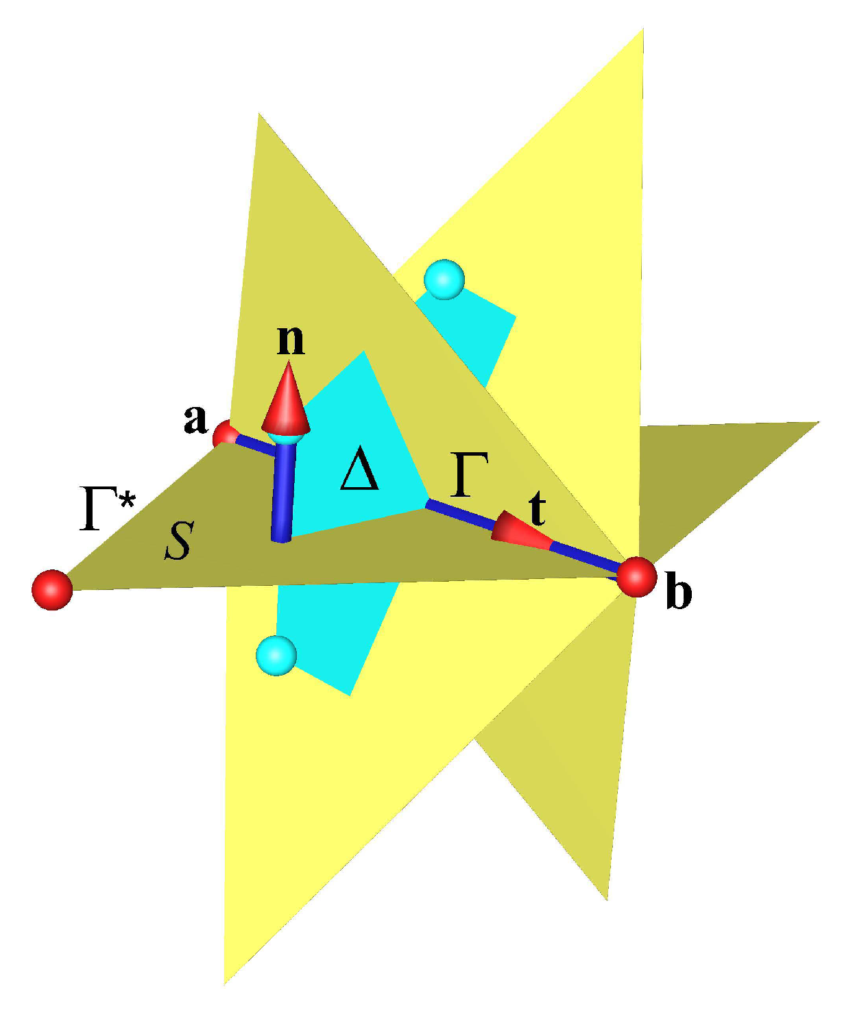
The extension to several dimensions of space is achieved by the construction of a discrete geometric structure based on the association of segments by their ends. Three segments build a triangular planar surface, but the planar polygonal surface can be generated from n segments; the collection of n segments forming the surface $\mathcal{S}$ is named ${\Gamma }^{*}$. Figure 1 shows the geometric structure made up of the different facets $\mathcal{S}$ having the principal segment $\Gamma$ in common.

Each facet has a normal $\mathbf{n}$ orthogonal to the direction of the unit vector $\mathbf{t}$, $\mathbf{n}·\mathbf{t}=0$. This set forms the local frame of reference whose position and directions in three-dimensional space are undefined. The changes of frames of reference of classical mechanics are no longer possible, the interactions from one segment to another are cause and effect, from the modification of the common scalar potential located on a vertex. This extension is limited to the creation of a polyhedral structure without any particular privileged direction, in particular the notion of volume is not necessary for the derivation of an equation of motion.

However, it should be considered that the only scalar potential $\varphi$ is not sufficient to characterize the intrinsic acceleration $\mathbf{\gamma }$. Indeed, the velocities on contour ${\Gamma }^{*}$ create a curl carried by the normal $\mathbf{n}$ to the facet $\mathcal{S}$; this axial vector $\mathbf{\psi }$ associated with that of all the other facets having the segment $\Gamma$ in common makes it possible to calculate a circulation on the contour of the dual surface $\Delta$ passing through the barycenters of the facets. This dual curl is carried by the segment $\Gamma$, thus defining a second contribution to the intrinsic acceleration $\mathbf{\gamma }$:

$$\begin{array}{c}\hfill {\displaystyle \mathbf{\gamma }=-\nabla \varphi +\nabla \times \mathbf{\psi }}\end{array}$$

(4)

The second contribution is orthogonal to the first because they cannot combine, they simply add up; exchanges between the two contributions are only possible if the acceleration $\mathbf{\gamma }$ is not zero. This observation is in line with J.C. Maxwell’s idea on the dynamic role of electromagnetic interactions [15]. Equation (4) is a formal Helmholtz–Hodge decomposition of the acceleration. The third harmonic term at the same time with divergence-free and curl-free does not exist here because it corresponds to the uniform translational and rotational movements immediately eliminated by the operators in accordance with the principle of relativity. The intrinsic acceleration $\mathbf{\gamma }=d\mathbf{V}/dt$ has a particular status; it is the only quantity that can be considered as absolute. As we perceive the direct actions represented by $\nabla \varphi$ and induced by $\nabla \times \mathbf{\psi }$ are entangled, in several dimensions of space one does not exist without the other, one is the dual of the other. The classical interactions of electromagnetism between direct currents and induced currents are exactly the same in mechanics. The formulation has a certain number of properties in particular the global and local orthogonality of the terms in gradient and in dual curl. The discrete operators mimic some properties of the continuous operators $\nabla \times (\nabla \varphi )=0$ and $\nabla ·(\nabla \times \mathbf{\psi })=0$ whatever the polygonal geometric structure, polygonal or polyhedral, structured or unstructured.

In discrete mechanics time runs smoothly from an instant $t^o$ to the current instant $t=t^o+dt$. There is no dilatation of time interval $dt$ no more than contraction of the lengths, these quantities are independent of the otherwise relative velocity. Relativistic effects are taken into account in completely different ways. The state of the system is completely defined at the instant $t^o$ from scalar and vector potentials of the acceleration, ${\varphi }^o$ and ${\mathbf{\psi }}^o$. The derivation of the discrete equation of motion therefore requires calculating the acceleration $\mathbf{\gamma }$ at the current state by the law (4).

2.3. Equations of Discrete Formulation

The calculation of the current potentials $\varphi$ and $\mathbf{\psi }$ must be modeled by the introduction of increments $d\varphi$ and $d\mathbf{\psi }$ dependent on the velocity $\mathbf{V}$ on each segment. The potentials ${\varphi }^o$ and ${\mathbf{\psi }}^o$ are called retarded potentials with reference to the Liénard–Wichert [16] potentials of electromagnetism. The acceleration then becomes $\mathbf{\gamma }=-\nabla ({\varphi }^o+d\varphi )+\nabla \times ({\mathbf{\psi }}^o+d\mathbf{\psi })$. The modeling of these terms, which given previously in [17], make it possible to write the discrete equation of motion in the form:

$$\begin{array}{c}\hfill \left\{\begin{array}{c}{\displaystyle \mathbf{\gamma }=-\nabla \left({\varphi }^o-dt{c}_l^2\nabla ·\mathbf{V}\right)+\nabla \times \left({\mathbf{\psi }}^o-dt{c}_t^2\nabla \times \mathbf{V}\right)+{\mathit{h}}_s}\hfill \\ \\ {\displaystyle (1-{\alpha }_l){\varphi }^o-dt{c}_l^2\nabla ·\mathbf{V}⟼{\varphi }^o}\hfill \\ \\ {\displaystyle (1-{\alpha }_t){\mathbf{\psi }}^o-dt{c}_t^2\nabla \times \mathbf{V}⟼{\mathbf{\psi }}^o}\hfill \\ \\ {\displaystyle {\mathbf{V}}^o+\mathbf{\gamma }dt⟼{\mathbf{V}}^o}\hfill \\ \\ {\displaystyle {\mathbf{U}}^o+\mathbf{V}dt⟼{\mathbf{U}}^o}\hfill \end{array}\right.\end{array}$$

(5)

where $c_l$ and $c_t$ are the longitudinal and transverse celerities; these quantities measured experimentally must simply be known. The source term ${\mathit{h}}_s$ here characterizes the other contributions to the modification of acceleration, gravitational effects, capillary effects, etc. The ⟼ symbol corresponds to an upgrade from time $t^o$ to time t. The quantities ${\alpha }_l$ and ${\alpha }_t$ are the attenuation factors of the longitudinal and transverse waves. In the case of a fluid, the shear stresses are relaxed in a very short time, of the order of $\tau \approx {10}^{-12}s$, and the attenuation factor ${\alpha }_t$ is then close to unity; a fluid does not retain the memory of the shear. On the contrary, an elastic solid medium has a zero attenuation factor ${\alpha }_t=0$ and the transverse waves persist for a very long time. In the general case, the two factors ${\alpha }_l$ and ${\alpha }_t$ are arbitrary.

The retarded potentials ${\varphi }^o$ and ${\mathbf{\psi }}^o$ are expressed in $m^2{s}^{-2}$ or energies per units of mass. System upgrades (5) correspond to the accumulation of compression and rotation energies and are also written in the form:

$$\begin{array}{c}\hfill {\displaystyle {\varphi }^o=-{\int }_0^{t^o}{c}_l^2\nabla ·\mathbf{V}d\tau ;{\mathbf{\psi }}^o=-{\int }_0^{t^o}{c}_t^2\nabla \times \mathbf{V}d\tau }\end{array}$$

(6)

The equation of discrete motion of system (5) is also a law of conservation of energy per unit mass. This consists of two Lagrangians where the kinetic and potential energies are exchanged separately for compression and shear. The interactions between the effects of compression and shear, on the other hand, can only be achieved by modifying the acceleration. The discrete formulation is a continuous memory model; the knowledge of the potentials at the instant $t^o$ and of the velocity $\mathbf{V}$ makes it possible to resume the forecast of the next state at any time.

Equation (5) makes it possible to investigate various problems of mechanics, the incompressible or compressible fluid flows, the mechanics of elastic solids or of media having complex constitutive laws but also the couplings with other phenomena such as thermal diffusion. The formulation lends itself to simulations carried out at all time scales, the product $dt{c}_l^2$ for the longitudinal effects or $dt{c}_t^2$ for the transverse effects indeed allow to take into account the characteristic scale of the phenomenon independently of its celerities. The treatment of a fluid is exactly the same as for a solid, only the physical characteristics $(c_l,c_t,{\alpha }_l,{\alpha }_t)$ are modified. The formulation is perfectly suited to fluid–structure interaction with large deformations.

2.4. Inertia on Discrete Formulation

The resolution of the system (5) is essentially unsteady, although it can be used to obtain a stationary solution if it exists by adopting a very large time interval in order to ensure $-\nabla \varphi +\nabla \times \mathbf{\psi }=$ 0. It is thus advisable to express the acceleration starting from the derivative in time and the nonlinear terms. These terms differ significantly from those of classical mechanics which are written in the form $\mathbf{V}·\nabla \mathbf{V}$ or $\nabla ·\left(\mathbf{V}\otimes \mathbf{V}\right)-\mathbf{V}\nabla ·\mathbf{V}$ or $\nabla \left(\right|\mathbf{V}{|}^2/2)-\mathbf{V}\times \nabla \times \mathbf{V}$. In discrete mechanics, inertial acceleration takes the form of a Helmholtz–Hodge decomposition [9]:

$$\begin{array}{c}\hfill {\displaystyle \mathbf{\gamma }=\frac{d\mathbf{V}}{dt}\equiv \frac{\partial \mathbf{V}}{\partial t}+\nabla {\varphi }_i-\nabla \times {\mathbf{\psi }}_i=\frac{\partial \mathbf{V}}{\partial t}+\nabla \left(\frac{{\parallel \mathbf{V}\parallel }^2}{2}\right)-\nabla \times \left(\frac{{\parallel \mathbf{V}\parallel }^2}{2}\mathbf{n}\right)}\end{array}$$

(7)

If the gradient term of the inertial potential ${\varphi }_i={\parallel \mathbf{V}\parallel }^2/2$ is the same as with continuous media, the last term is a true dual curl. Applying the divergence operator to the equation of motion eliminates this term, which is not the case in the mechanics of continuous media. In some cases, it is possible to pass the term in gradient of the inertial potential in the second member to reveal the potential of Bernoulli, ${\varphi }_B^o={\varphi }^o+{\varphi }_i$. The solution of the velocity problem does not depend on the scalar potential used and this operation makes it possible to reduce the discretization errors, in particular for turbulent flows where inertia plays an important role. Writing in the form (7) of inertia makes it possible to make this equation of motion completely symmetrical thanks to the Helmholtz–Hodge decomposition by making possible the regrouping of the terms in gradient and in dual curl.

2.5. Reduction to Waves Equation

The strong coupling between the shear stresses defined by $\nabla \times \mathbf{\psi }$ and compression represented by $-\nabla \varphi$ necessarily passes through the acceleration $\mathbf{\gamma }=-\nabla \varphi +\nabla \times \mathbf{\psi }$. Indeed, the two operators gradient and dual curl are orthogonal and cannot directly exchange energy. We can show that the vector Equation (5) is a wave equation. Consider the special case where $c_l=c_t=c$ and apply the Leibniz calculus formula:

$$\begin{array}{c}\hfill {\displaystyle {\nabla }^2\mathbf{V}=\nabla \nabla ·\mathbf{V}-\nabla \times \nabla \times \mathbf{V}}\end{array}$$

(8)

By using the definition of the displacement $\mathbf{U}={\mathbf{U}}^o+\mathbf{V}dt$, we obtain a form which contains the retarded potentials at the second member:

$$\begin{array}{c}\hfill {\displaystyle \frac{d^2\mathbf{U}}{d{t}^2}-c^2{\nabla }^2\mathbf{U}=-\nabla {\varphi }^o+\nabla \times {\mathbf{\psi }}^o}\end{array}$$

(9)

The first member of this equation is a d’Alembertian $☐\mathbf{U}$:

$$\begin{array}{c}\hfill {\displaystyle \frac{1}{c^2}\frac{{\partial }^2\mathbf{U}}{\partial t^2}-{\nabla }^2\mathbf{U}}\end{array}$$

(10)

In solid mechanics, the celerities $c_l$ and $c_t$ are generally of the same order of magnitude but not equal. The system (5) generalizes the wave propagation equation, in a homogeneous medium or in a vacuum in the case of electromagnetism, to any medium, fluid or solid with complex constitutive laws and for anisotropic media. In the general case, the celerities depend on other variables such as temperature, time or of course the constraints themselves. For fluids, the transverse celerity $c_t$ can be considered as zero because the relaxation times of the shear stresses are very short, of the order of ${10}^{-12}$ s; the shear stress takes the instantaneous value ${\mathbf{\psi }}^o=-\nu \nabla \times \mathbf{V}$ where $\nu$ is the kinematic viscosity. The value of the attenuation factor ${\alpha }_t$ of the transverse waves is then equal to the unit. At very low time constants, the fluid behaves as a solid of celerity $c_t$, which makes it possible to remove the paradox of the Stokes equation where, for an imposed shear, the stress is infinite at the initial time.

3. Numerical Methodology

The resolution of the vector equation of the system (5) is carried out on the support of a primal geometry of finite element type constructed from elements similar to the stencil of Figure 1. The structured or unstructured polygonal or polyhedral mesh with any number of facets is characterized by the number of vertices $n_v$, the number of facets $n_f$ and the number $n_e$ of segments $\Gamma$ on which is assigned the velocity variable or rather its components.

The numerical methodology implemented to simulate the various flows or FSI problems is very close to the mimetic methods initiated by Shaskhov [12] for the diffusion equation; since then, they have been applied successfully to different fields of physics, mechanics, electromagnetism, etc. This method is formally very close to the ideas retained for the discrete physical model itself; the connection between the two has been highlighted recently [11]. This methodology is of the ready-to-use type; indeed, no discretization is necessary to transform the discrete vector equation into an algebraic system of rank $n_e$. The gradient operator $\nabla \varphi$ represents the component of the gradient vector on the segment $\Gamma$, which is simply calculated by $\nabla \varphi =({\varphi }_b-{\varphi }_a)/dh$. The primal curl $\nabla \times \mathbf{V}$ is evaluated from the velocity circulation along the ${\Gamma }^{*}$ contour. The divergence of the velocity $\nabla ·\mathbf{V}$ is represented by the sum of all flows associated with a vertex of the primal mesh. Finally, the dual curl $\nabla \times \mathbf{\psi }$ is calculated from the circulation of this vector on the dual contour passing through the barycenters of the facets. The only $n_e$ unknowns are the velocity components on the segments $\Gamma$. Solving the corresponding linear system by a method of conjugated gradients, preconditioned or not, or even by a direct method, makes it possible to extract the values of $\mathbf{V}$. The upgrade of the potentials ${\varphi }^o$ and ${\mathbf{\psi }}^o$ is carried out explicitly using the operators $\nabla ·\mathbf{V}$ and $\nabla \times \mathbf{V}$. The time integration is carried out by a Gear diagram of order one or two. The nonlinear terms $\nabla (\parallel \mathbf{V}{\parallel }^2/2)$ and $\nabla \times (\parallel \mathbf{V}{\parallel }^2/2\mathbf{n})$ are treated in a semi-implicit way by writing ${\parallel \mathbf{V}\parallel }^2={\mathbf{V}}^n·{\mathbf{V}}^{n+1}$ where n is the exponent representing the time step.

The formulation has some properties including that of mimicking those of continuous operators, i.e., ${\nabla }_h\times \left({\nabla }_h\varphi \right)=0$ and ${\nabla }_h·({\nabla }_h\times \mathbf{\psi })=0$, and this whatever the nature of the mesh adopted. Another very important property is the discrete local and global orthogonality of $\nabla \varphi$ and $\nabla \times \mathbf{\psi }$ demonstrated in [8]. In the case of a regular mesh, these properties combine to exhibit a spatial convergence to the second order in all cases previously treated with the aid of this formulation.

4. Verifications

The following very simple test cases have analytical solutions which make it possible to check that the results of the discrete Equation (5) are indeed in conformity with those of the continuum mechanics despite a significantly different formulation. These examples also serve to explain the role of each discrete operator by dissociating the effects of compression from those of rotation.

4.1. Shear between a Fluid and an Elastic Media

We consider one of the simplest cases of fluid–structure interaction to study the behavior of two media, one viscous and the other elastic. This test case has a very simple analytical solution that highlights the behavior of the two media modeled with the discrete description (5). The domain height h = 1 m is separated by a $\Sigma$ interface located at $h/2$. The velocity of the lower wall is kept at rest and the upper surface is initially set in motion with a velocity $V_0$ = 1 m s${}^{-1}$.

Let us first consider the purely viscous case of two kinematic viscosity fluids ${\nu }_1$ = 1 m${}^2$ s${}^{-1}$ and ${\nu }_2$ = 4 m${}^2$ s${}^{-1}$; the solution obtained using the system (5) converges very quickly towards the stationary solution. It appears as two right-hand portions satisfying the boundary conditions and the condition ${\nu }_1\nabla \times {\mathbf{V}}_1={\nu }_2\nabla \times {\mathbf{V}}_2$ at the interface. Under these conditions, the velocity at the interface is equal to $V_i=0.2$. The 1D solution does not depend on the chosen spatial approximation and the error is zero to almost machine accuracy. Note that the condition at the interface is implicitly provided by the $\nabla \times \left(\nu \nabla \times \mathbf{V}\right)$ operator. The constant rotational in each medium is, respectively, equal to $\nabla \times {\mathbf{V}}_1=-1.6$ and $\nabla \times {\mathbf{V}}_2=-0.4$. Since the problem has no compressibility terms, only the viscous terms independent of the first ones appear in the discrete motion equation.

The lower part of the domain is now assumed to behave as an elastic solid of celerity $c_t^2=\nu =4$. The upper part is occupied by a fluid whose viscosity is equal to $\nu =1$. The potential vector ${\mathbf{\psi }}^o$ makes it possible to accumulate the shear stresses in the solid, the constraints at the interface in the fluid being effectively transmitted and stored in the solid. The solution converges rapidly to a strictly zero velocity field in the solid and a linear velocity profile satisfying the condition in $y=h$ and at zero velocity on the $\Sigma$ interface. The vector equation of the system (5) is identically satisfied with ${\mathbf{\psi }}^o=\nu \nabla \times \mathbf{V}$ where $\mathbf{V}$ is the velocity of the fluid and ${\mathbf{\psi }}^o=2$. The exact solution does not depend on the spatial approximation.

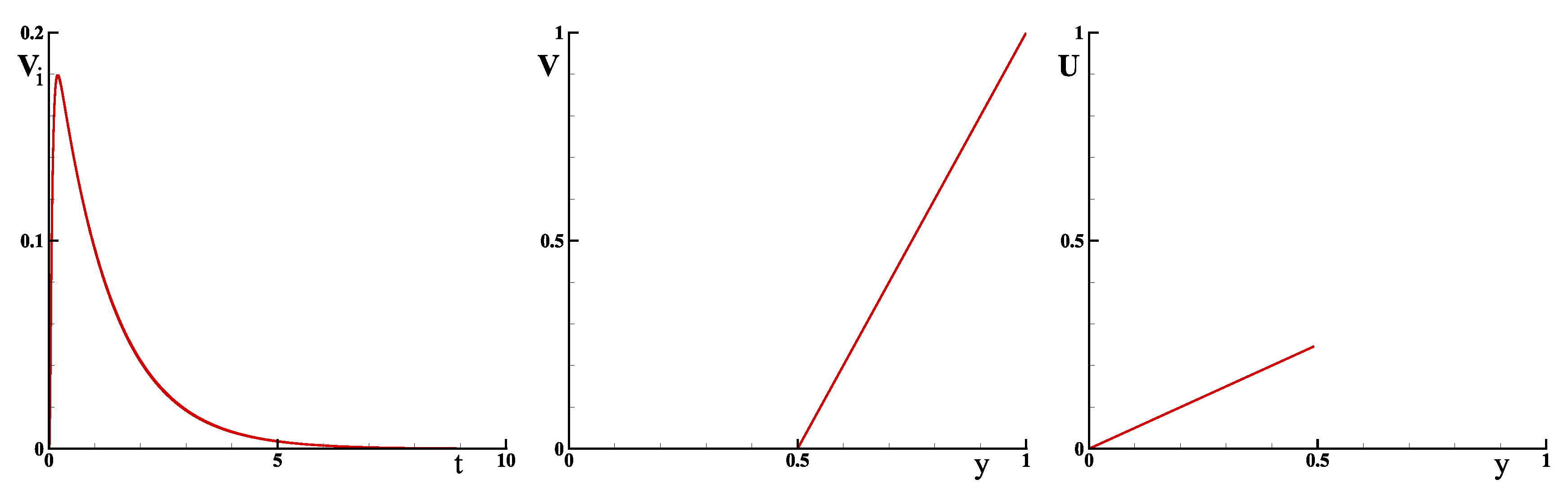
Figure 2 shows the evolution of the velocity at interface $\Sigma$ over time. It diminishes quickly, enough to become zero. The velocity field is zero in the solid and linear in the steady-state fluid. The figure also gives the displacement $\mathbf{U}$ of the solid at the end of the time evolution.

While a fluid moves indefinitely under the action of shear, an elastic solid quickly reaches a stationary displacement. The absence of interpolation at the interface between a fluid and a solid allows us to reach the exact solution. This very simple example makes it possible to understand the different mechanisms involved in Equation (5) and to validate the unsteady and stationary fluid–solid interaction.

In continuum mechanics, the theoretical solution of this problem can be obtained by considering the two media separately by imposing boundary conditions at the interface. The equations, in a stationary incompressible regime without inertial effects, for the fluid and solid media are, respectively:

$$\begin{array}{c}\hfill \left\{\begin{array}{c}{\displaystyle \nabla ·\left({\nu }_f\left(\nabla \mathbf{V}+{\nabla }^t\mathbf{V}\right)\right)=0}\hfill \\ \\ {\displaystyle \nabla \times \left({\nu }_s\nabla \times \mathbf{U}\right)=0}\hfill \end{array}\right.\end{array}$$

(11)

When the properties ${\nu }_f$ and ${\nu }_s$ are constant, these equations are reduced to Laplacian terms. With the assumptions adopted here, the results in the fluid are obtained with the Navier–Stokes equation, while the solid solutions come from the Navier–Lamé equation. The conditions at the interface are simple, for the fluid the velocity is zero at $y=h/2$, while its value is $V_0$ at $y=h$. For the solid, the displacement is null at $y=0$ and the constraint is imposed at the interface $y=h$, chosen equal to that of the fluid side. The velocity is of course zero in the solid domain. The solution is very simple: $v\left(y\right)=\mathbf{V}·e_x=\left(2y/h-1\right)$ and $u\left(y\right)=\mathbf{U}·e_x={\nu }_f/{\nu }_s(2y/h)$. As expected, the velocity solution $v\left(y\right)$ does not depend on viscosity, whereas the displacement depends on the ratio ${\nu }_f/{\nu }_s$. For this simple problem, the solutions of discrete mechanics are of course the same as in continuum mechanics. Among the advantages of the monolithic discrete approach, the equation of motion is unique for all media. Its acceleration formulation makes it possible to consider velocity and displacement as simple accumulators associated with operators $\nabla ·\mathbf{V}$ and $\nabla \times \mathbf{V}$.

4.2. Compression of an Elastic Solid by a Fluid

Consider the case of a square cavity of dimension $[0,1]\times [0,1]$ filled with two media: (i) a fluid of density ${\rho }_1$ = 1.1768 kg m${}^{-3}$ in the upper half; and (ii) a solid of density ${\rho }_2$ = 1.1768 kg m${}^{-3}$ in the lower part. The longitudinal velocity of the fluid considered as an ideal gas is equal to $c_l$ = $\sqrt{r{T}_0}$ m s${}^{-1}$ where $T_0$ is the constant temperature of the whole system; the celerity of the solid is imposed as $c_l$ = 5000 m s${}^{-1}$. The evolution is therefore considered as isothermal.

At the instant $t=0$, we inject air at the velocity $V_0=-0.01{\mathbf{e}}_y$ whose density is equal to ${\rho }_0={\rho }_1$ by the upper surface. The divergence of the velocity is uniform and constant over time and equal to $\nabla ·\mathbf{V}=-V_{0}S/[\Omega ]$. The compression of the fluid is homogeneous taking into account the very slow variations of the variables; the density as the pressure are uniform in each of the two domains. As the walls of the cavity are strictly rigid, the compression of the solid is uniaxial. The effects of shearing are strictly null. The system (5) reduces to the following equations:

$$\begin{array}{c}\hfill \left\{\begin{array}{c}{\displaystyle \mathbf{\gamma }=-\nabla \left({\varphi }^o-dt{c}_l^2\nabla ·\mathbf{V}\right)}\hfill \\ \\ {\displaystyle {\varphi }^o-c_l^{2}dt\nabla ·\mathbf{V}⟼{\varphi }^o}\hfill \end{array}\right.\end{array}$$

(12)

The classic solution of this problem in the concept of continuous media, obtained by considering the evolution as isothermal and the gas as ideal, is simple and gives the evolutions of the variables of the problem as a function of time:

$$\begin{array}{c}\hfill \left\{\begin{array}{c}{\displaystyle p_1\left(t\right)=p_0\left(1-\nabla ·\mathbf{V}t\right)}\hfill \\ \\ {\displaystyle {\rho }_1\left(t\right)={\rho }_0\left(1-\nabla ·\mathbf{V}t\right)}\hfill \end{array}\right.\end{array}$$

(13)

where ${\rho }_0$ = 1.1768 kg m${}^{-3}$ is the density of the injected fluid and $p_0$ is equal to $1.0135·{10}^5\mathrm{Pa}$.

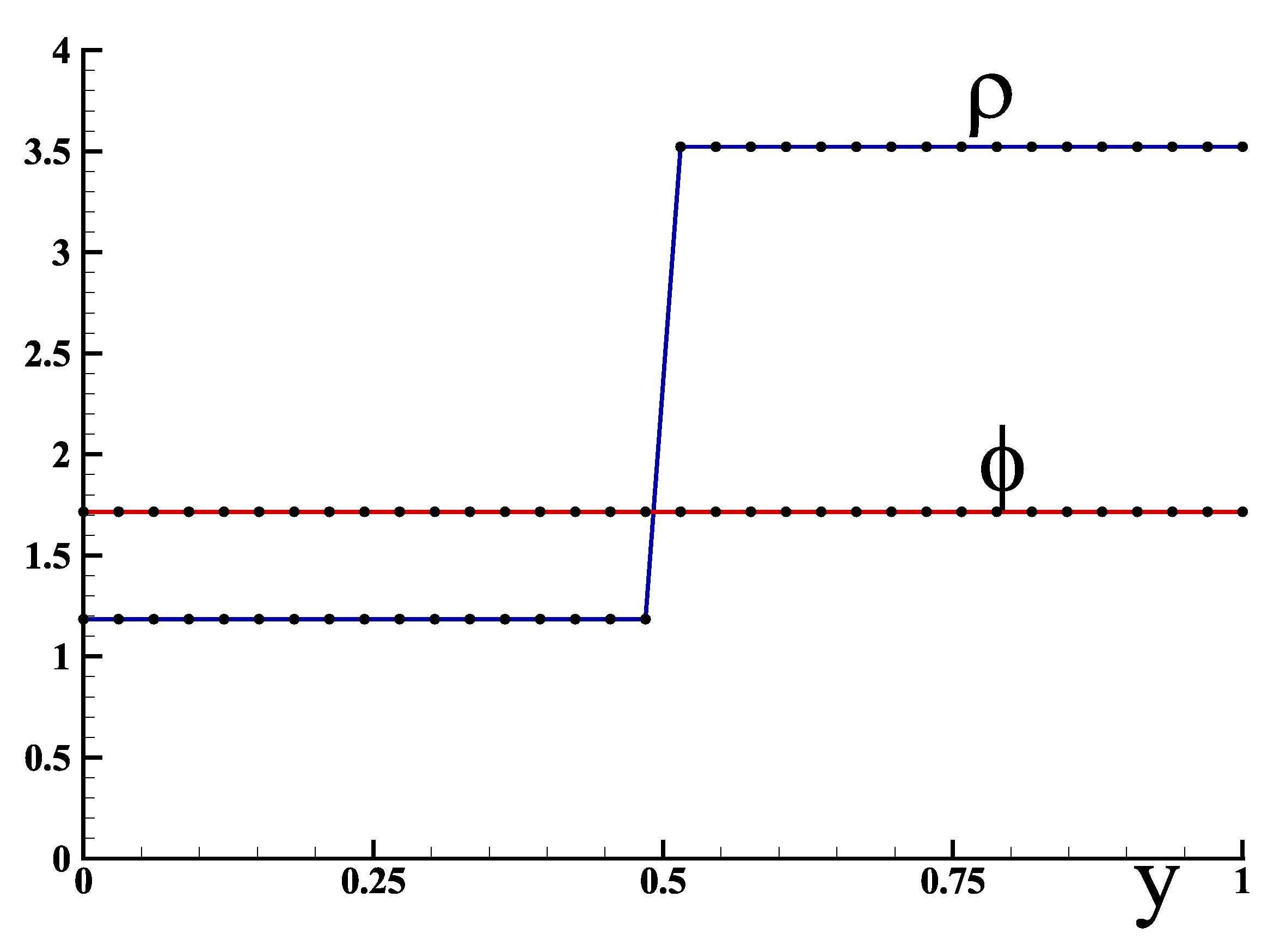
In discrete mechanics the variables of the problem are $(\mathbf{V},{\varphi }^o)$. The pressure p and the density $\rho$ are replaced by the single variable ${\varphi }^o$ but these two quantities can possibly be calculated a posteriori by an integration in time of the divergence of the velocity used to upgrade the scalar potential. The problem is solved from the system (12) and initial conditions $(\mathbf{V}=0,{\varphi }^o=0)$. Figure 3 shows the solution obtained at the end of a simulation time of t = 100 s according to the vertical coordinate y. The scalar potential ${\varphi }^o$ and the density $\rho$ evolve linearly over time.

At the end of the simulation, the density in the fluid is equal to $\rho$ = 3.5224 kg m${}^{-3}$ and that of the solid is equal to $\rho$ = 1.1849 kg m${}^{-3}$. The value of the potential is strictly constant in the whole domain and equal to 1.7161 · 10${}^5$ m${}^2$ s${}^{-2}$. The density of the fluid increased according to the isothermal compression law of an ideal gas while that of the solid only varied by $\Delta \rho$ = 0.0081 kg m${}^{-3}$. These values correspond to the theoretical solution of the problem.

As shown in Figure 3, the scalar potential is uniform in the cavity; this means that the energy produced by the injection of the fluid is distributed uniformly in the solid and the fluid. The concept of pressure that could possibly be given depends on the definition given to it; if we adopt the law $p={\rho }_0{\varphi }^o$ then it will also be uniform in the two media. In fact, this distinction is inconsequential because the pressure p has no influence on the solution of the problem; it is only a secondary variable which one can do without.

In conclusion, this case of isothermal uniaxial compression treated using the equation of discrete mechanics (5) allows finding the exact solution provided by the mechanics of continuous media. The discrete equation is both an equation of motion and a law of conservation of mechanical energy, compression and shear.

5. Validation

The validations of the discrete formulation in its previous version were carried out on standard test cases from the literature (e.g., [6,7]). More recent cases [8] have validated the current form of discrete equations on the FSI in addition to more specific examples devoted to the inertial term [9] or heat transfer at small scales. The case presented here is one of the benchmarks often used in FSI.

Lid-Driven Open Cavity Flow with Flexible Bottom Wall

The lid-driven cavity with flexible bottom is an example that we can reasonably deal with. This case corresponds to that proposed in [13]. It was also considered by others authors [2,14]. A fluid, characterized by its kinematic viscosity $\nu$ = 10${}^{-2}$ m${}^2$ s${}^{-1}$, is driven by the velocity boundary condition of the top of the cavity which varies with time: $u(x,t)=1-cos(2\pi t/T)$, where the period is equal to T = 5 s.

The elastic structure density is ${\rho }_s$ = 500 kg${}^{-1}$ m${}^{-3}$, the Young’s modulus is E = 250 Pa and the Poisson coefficient is $\sigma =0$. The fluid is considered as incompressible. Neumann boundary conditions are imposed on the two holes localized at the top of the vertical walls. As we resolve at the same time the velocity field and the displacement field in the fluid and the elastic membrane, respectively, using a fixed grid, we have to take a relatively large thickness for the membrane (2% of the cavity length) compared to other simulations of the literature, in order prevent a use of a very fine grid. The solution is obtained from zero fields from the system of Equation (5).

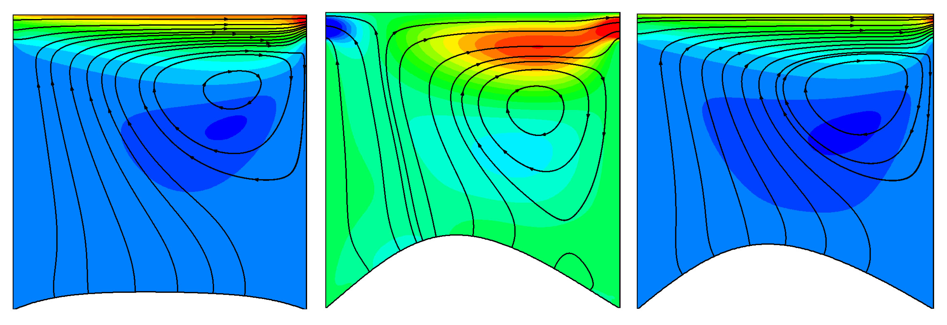
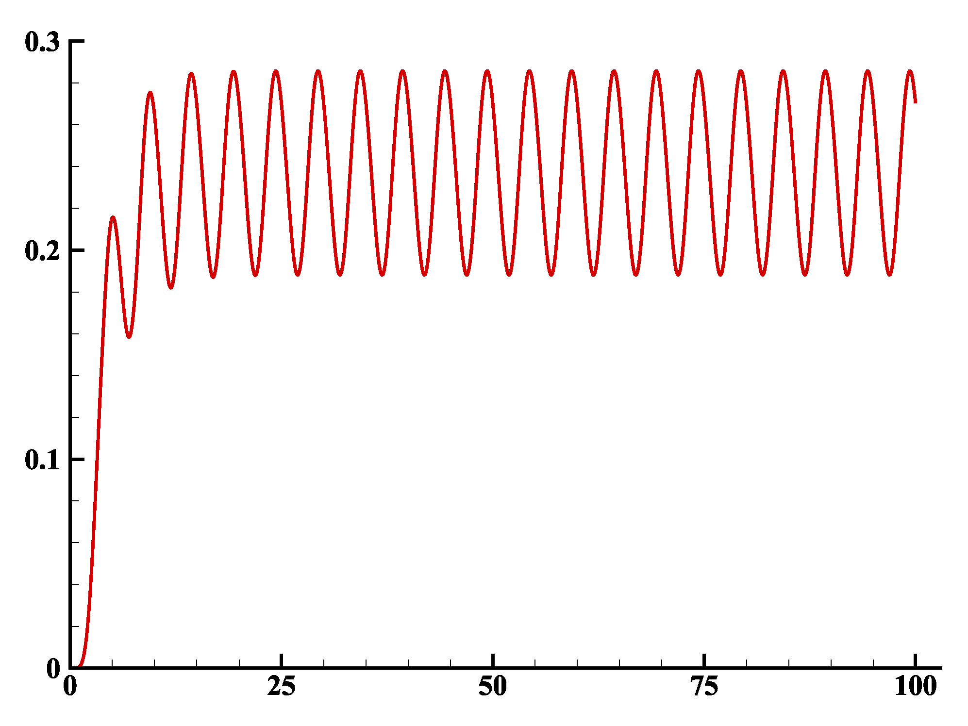
The differential discrete operators, such as gradient, divergence and rotational properties have the properties of continuum $\nabla ·\nabla \times \mathbf{\psi }=0$ and $\nabla \times \nabla \varphi =0$ on every type of unstructured polyhedral meshes. This methodology is similar to what is proposed in the discrete exterior calculus [5]. In the present case, adaptive quadrangle mesh is used with initially 2562 cells. The resolution of the motion equation of the fluid allows obtaining the pressure on the top surface of the membrane, the lower surface being maintained at a constant pressure $p=0$. The force acting on the membrane, proportional to the pressure difference, allows to calculate its displacement. The mesh is then modified at each time step. This is what we call the Arbitrary Lagrangian Eulerian method. The results obtained are presented in Figure 4 where the horizontal velocity maps in the fluid and the membrane shape are shown together with the streamlines for different time steps. After an unsteady phase of a few cycles, the regime becomes totally periodic, of period T = 5 s (Figure 5). The divergence of the velocity remains less than ${10}^{-8}$ throughout the calculation. The celerity of air, which is equal to $c\approx$ 340 m s${}^{-1}$, maintains the flow in the incompressibility approximation for the selected time period $dt$ = 10${}^{-2}$ s. Indeed, the discrete model clearly shows that the Mach number $M=v/c$ does not define the incompressibility of a flow: this is the product $dt{c}_l^2$. For example, water, an essentially incompressible fluid, propagates the waves at a celerity of $c_l\approx$ 1500 m s${}^{-1}$, which induces the fact that water is a compressible medium if the observation time constant $dt$ is sufficiently low.

Depending on the author, the results may be different; the cavity can be globally suppressed with respect to the outside, this is the case for the work of Bathe [1] where the vertical positions of the membrane are alternately positive and negative. The comparison with the previous simulations by Gerbeau [13] or Kassiotis [14] are on the other hand in good qualitative agreement with those obtained in this study; the amplitude of the variations of the position of the membrane is close to that of these authors and the position of the interface always positive. The form of bottom flexible wall at different times corresponds well to that shown by Kassiotis [14] despite very different numerical methodologies.

The case of rigid lid-driven cavity flow was compared very precisely with the results of Bruneau et al. [18]. In general, the numerical methodology associated with the discrete model is of order two in space and time; in parallel, the fluid structure coupling also showed that this precision could be maintained [8] for the analytical solution of Sugiyama [10]. The differences however reduced in the case presented here with those of Kassiotis are explained by differences in the treatment of the fluid–structure coupling.

6. Conclusions

The unique discrete Formulation (5) to represent the motions of fluids and the displacements of solids in large deformations has the advantage of allowing a monolithic treatment of fluid–structure interaction. The celerities $c_l$ and $c_t$ and the attenuation factors of the waves ${\alpha }_l$ and ${\alpha }_t$ make it possible to describe all the phenomena including for complex constitutive laws. The state laws of the mediums and their rheological laws are not part of the system of equations; only the four physical parameters depending on time and space allow modifying the local state of the medium. The double representation in velocity $\mathbf{V}$ and displacement $\mathbf{U}$ makes the computation of the compression and shear stresses possible; these constraints are the respective energies per unit mass. Thus, the total energy is strictly conserved during a simulation.

The unification of the laws of fluid and solid mechanics can be extended to the propagation of waves of all kinds: swells, sound waves, shock waves, electromagnetism, etc. The equation of motion thus becomes an equation of waves where only acceleration is at the origin of transformations from one form of energy to another. The principle of relativity applied to velocity and acceleration induces invariances respected by the discrete equation of motion.

References

- Bathe, K.-J.; Zhang, H. Finite element developments for general fluid flows with structural interactions. Int. J. Numer. Methods Eng. 2004, 60, 213–232. [Google Scholar] [CrossRef] [Green Version]
- Bathe, K.-J.; Zhang, H. A mesh adaptivity procedure for cfd and fuid-structure interactions. Comput. Struc. 2009, 87, 604–617. [Google Scholar] [CrossRef]
- Hyman, J.; Shashkov, M. Natural discretizations for the divergence, gradient ans curl on logically rectangular grids. SIAM J. Num. Anal. 1999, 36, 788–818. [Google Scholar] [CrossRef] [Green Version]
- Hyman, J.; Shashkov, M. The orthogonal decomposition theorems for mimetic finite difference methods. SIAM J. Num. Anal. 1999, 36, 788–818. [Google Scholar] [CrossRef] [Green Version]
- Desbrun, M.; Hirani, A.; Leok, M.; Marsden, J. Discrete exterior calculus. arXiv 2005, arXiv:0508341v2. [Google Scholar]
- Bordère, S.; Caltagirone, J.-P. A unifying model for fluid flow and elastic solid deformation: A novel approach for fluid structure interaction. J. Fluid Struct. 2014, 51, 344–353. [Google Scholar] [CrossRef]
- Bordère, S.; Caltagirone, J.-P. A multi-physics and multi-time scale approach for modeling fuid-solid interaction and heat transfer. Comput. Struc. 2016, 164, 38–52. [Google Scholar] [CrossRef]
- Caltagirone, J.-P.; Vincent, S. On primitive formulation in fluid mechanics and fluid-structure interaction with constant piecewise properties in velocity-potentials of acceleration. Acta Mech. 2020, 231, 2155–2171. [Google Scholar] [CrossRef] [Green Version]
- Caltagirone, J.-P. On Helmholtz-Hodge decomposition of inertia on a discrete local frame of reference. Phys. Fluids 2020, 32, 083604. [Google Scholar] [CrossRef]
- Sugiyama, K.; Ii, S.; Takeuchi, S.; Takagi, S.; Matsumoto, Y. A full eulerian finite difference approach for solving fluid-structure coupling problems. J. Comput. Phys. 2011, 230, 596–627. [Google Scholar] [CrossRef] [Green Version]
- Caltagirone, J.-P. Application of discrete mechanics model to jump conditions in two-phase flows. J. Comp. Phys. 2021, 432, 110151. [Google Scholar] [CrossRef]
- Shaskov, M. Conservative Finite-Difference Methods on General Grids; CRC Press: Boca Raton, FL, USA, 1996. [Google Scholar] [CrossRef]
- Gerbeau, J.; Vidrascu, M. A quasi-newton algorithm based on a reduced model for fluid-structure interaction problems in blood flows. Math. Model. Numer. Anal. 2003, 37, 631–647. [Google Scholar] [CrossRef] [Green Version]
- Kassiotis, C.; Ibrahimbegovic, A.; Niekamp, R.; Matthies, H. Nonlinear Fluid-Solid-driven cavity flow with flexible bottom structure problem, Part I: Implicit partitioned algorithm, nonlinear stability proof and validation examples. Comput. Mech. 2011, 47, 305–323. [Google Scholar] [CrossRef] [Green Version]
- Maxwell, J. A dynamical theory of the electromagnetic field. Philos. Trans. R. Soc. Lond. 1865, 155, 459–512. [Google Scholar]
- Liénard, A. Champ électrique et magnétique produit par une charge électrique concentrée en un point et animée d’un mouvement quelconque. L’Éclairage Électrique 1898, 27, 5–112. [Google Scholar]
- Caltagirone, J.-P. Discrete Mechanics, Concepts and Applications, ISTE; John Wiley & Sons: London, UK, 2019. [Google Scholar] [CrossRef]
- Bruneau, C.; Saad, M. The lid-driven cavity problem revisited. Comput. Fluids 2006, 35, 326–348. [Google Scholar] [CrossRef]
Figure 1.
Discrete geometric structure: a set of primitive planar facets are associated with the segment of unit vector whose ends a and b are distant by a length d. Each facet is defined by a contour , a collection of three segments , is oriented according to the normal such that ; the dual surface connecting the centroids of the cells is also flat.
Figure 2.
Fluid–structure interaction between a viscous fluid and an elastic solid; the viscosity of the fluid is equal to = 1 m s and the solid shear modulus is equal to = 4 m s: (left) the velocity of the interface over time is presented; (middle) the velocity at steady-state regime is reported; and (right) the displacement of the solid is plotted.
Figure 3.
Evolutions of the density and of the scalar potential as a function of the vertical coordinate y for a time s and an injection velocity = −0.01 m s for a mesh of cells.
Figure 4.
Vertical displacement at mid-point of flexible plate in lid-driven open cavity flow with flexible bottom wall, velocity and streamlines at t = 2.5, 15, 20 s.