Multiscale Filtering of Compressible Wave Propagation in Complex Geometry through a Wavelet-Based Approach in the Framework of Pressurized Water Reactors Depressurization Transient Analysis

Abstract

The proposed research takes place in the framework of the analysis of the mechanical consequences of accidental scenarios for pressurized water reactors (PWR). It is particularly dedicated to the effects of the propagation of a transverse rarefaction wave through the assemblies of the nuclear core, consecutive to a pipe break in the primary circuit of the reactor. This paper focuses on the representation, with a reduced number of well-chosen variables, of a pressure wave propagating through a highly congested medium composed of rod bundles, with the primary objective of accurately evaluating the resulting pressure forces exerted on the rods. To achieve this goal, a description of the fluid domain as a homogenized or porous medium is introduced, yielding the need for a new filtering technique to be applied to the fluid fields. A new homogenized and multiscale representation of the fluid variables, based on continuous wavelet transform (CWT), is thus proposed. The capabilities of CWT to accurately approximate a reference representative unsteady pressure field, corresponding to a wave propagation at microscale, is assessed. The proposed technique is applied to a pressure field obtained numerically at local scale. The number of variables that shall be kept at macroscale to have a meaningful representation of the pressure field is fully evaluated through the comparison of the fluid force applied to the microstructure.

1. Introduction

The present paper can be positioned in the framework of the analysis of the mechanical consequences of accidental scenarios for pressurized water reactors (PWR) and is particularly dedicated to the effects of the propagation of a transverse rarefaction wave through the assemblies of the nuclear core, consecutive to a pipe break in the primary circuit of the reactor. In this context, we are interested in the response of a set of fuel assemblies, composed of guide tubes and grids supporting fuel rods, to the dynamic loading induced by the pressure wave, the resulting internal constraints and deformations being the quantities to monitor in the end. This paper thus focuses on the representation, with a reduced number of well-chosen variables, of a wave propagating through a highly congested medium composed of rod bundles, with the primary objective of representing the resulting pressure forces exerted on the fuel assemblies in the most condensed form to then apply an equivalent beam model to the structure. This topic is a key component towards the design of a coupled fluid-structure solver implementing the proposed approximation of the fluid physical fields in these conditions.

Vibration phenomena under fluid loading are encountered in many industrial or research fields, such as aeronautics, biology, civil or nuclear engineering. However, addressing the topics introduced above with classical approaches relying on an explicit representation of the interfaces between fluid and solid will inevitably lead here to unaffordable computations. This often yields some strong simplifications, like in [1], where the interaction between a rarefaction wave originating from a pipe break and the core dynamics was studied with fuel assemblies considered as an equivalent acoustic impedance, responsible for the global pressure drop through the core. The proposed improvement is to add the representation of the fluid domain as a homogenized or porous medium, depending on the technique used to describe the effects of the local geometric details without explicitly representing them. Such a strategy has already been successfully implemented in the PWR framework in [2,3] in the case of a dynamic excitation related to seism. In these conditions, the fluid forces acting on structures come from the incompressible, turbulent, and mostly axial flow through the assemblies and are very different in nature from the pressure forces associated to waves in a compressible medium that are addressed in the present paper for a depressurization transient. In particular, the porous model for seismic transient does not account for transverse pressure gradient within the rod bundles, irrelevant with incompressible flow and yet mandatory in the situation of the current paper. A proper representation of the pressure wave loading at the suitable scale is therefore needed in order to then implement a beam-like model for fuel assemblies, in which the fluid forces acting on structures are derived from the local pressure field only, due to the inviscid interaction between fluid and structure coming with compressible models (i.e., Euler equations are used instead of Navier–Stokes equations). The representation of inner pressure gradients also introduces a multiscale problematics specific to the new framework of the present article, which significantly influences the choice of the filtering strategy needed to build the relevant set of variables representing the fluid at macroscale (i.e., one fuel assembly).

Considering the key ideas introduced above and the wide state of the art provided in the following section, the authors hereafter set the bases of a new homogenized and multiscale representation of the fluid variables, based on continuous wavelet transform (CWT). The added value of this research is thus the demonstration of the capabilities of CWT to, on the one hand, accurately approximate a reference representative unsteady pressure field corresponding to a wave propagation at microscale and, on the other hand, provide a physics-driven measure of this accuracy with respect to the number of variables conserved at macroscale, based on the evaluation of the resulting pressure force exerted on the rods.

This article is hereafter divided into five parts. In Section 2, a brief overview of the state-of-the-art on homogenized and multiscale approaches is presented, completed with some reference works on wavelet methods. In Section 3, the fluid and structure physical systems to consider are described, with a focus on the fluid problem and a brief presentation of the solid medium. In Section 4, the wavelet-based homogenized and multiscale filtering of the fluid fields is introduced, in order to build a set of macroscale variables describing the relevant information contained in local fields, whereas the capabilities of the CWT filtering in the proposed context are thoroughly tested and discussed in Section 5. The filtering technique is thus applied to a reference pressure field obtained numerically at local scale using EUROPLEXUS software for Euler equations (http://www-epx.cea.fr), and the accuracy of the approach in terms of conserved scales in the wavelet approximation, directly related to the number of variables kept at macroscale, is evaluated through the computation of the fluid force applied to the microstructure. The last section draws some conclusions and prospects of the proposed work.

To end this introduction, it is important to note that the proposed filtering technique only needs to be applied in a 2D geometry to match the requirements of the 3D analysis of the consequences of a depressurization in a PWR. Indeed, fuel assemblies exhibit a microstructure to be accounted for only in a transverse section, whereas the components of the waves along the axial direction can be described using standard discretization techniques (see Figure 1a for an overview of the major geometric characteristics of a PWR fuel assembly). The grids contribute little to the response of the assemblies to a transverse wave, and classical regular and singular head loss models can be implemented to account for them and for the friction along the rods for the axial component of the waves. Therefore, the 2D reference solution used in Section 5, which considers the 2D section of a $10\times 10$ rod bundle with relative dimensions in accordance with those of a PWR fuel assembly, is fully representative of the wave propagation problem to consider in the design of a dedicated homogenized porous approach.

2. Short Review of Homogenized or Filtered Approaches, and Wavelet Methods

Before going further in this article, it is important to note that the current work, while being applied in a particular industrial context, cannot be separated from the wide state-of-the-art on homogenization and multiscale methods involving fluids providing loads onto structures. Indeed, representing the main interaction phenomena occurring when a fluid flows inside a congested structural domain can be seen as a porous [3] or a homogenization problem [4]. In literature, classical (and analytical) homogenization techniques are based either on a representative volume element (in micromechanics) or on a periodic microstructure satisfying a scale separation assumption (in asymptotic homogenization). As for porous media approaches, they rely on a spatial averaging of local balance equations, initially defined on separated media [5,6]. Such a spatial filtering process can also be found, for instance, in multiphase flow literature [7] and in turbulence literature [8,9,10] with large eddy simulation (LES). All these different filtering or homogenization methods have in common the ability to simplify local geometry and small-scale phenomena, thus allowing to significantly reduce computation time. Nevertheless, they also do share the same limitations, that is to say, the treatment of boundary conditions, the loss of microscopic information, and the resulting need of closure model between resolved and unresolved scales.

All these different methods, connected within the wide family of multiscale modeling, could be even linked to the more general issue of reduced-order modeling and sparse representation of information. When studying either heterogeneous materials, multiphase or turbulent flows, or computing large scale systems, a fine representation of microscopic behavior is often too cumbersome. From a modeling point of view, this calls for the definition of mesoscopic or macroscopic variables and equations able to simulate an acceptable approximation of a system behavior. From a numerical point of view, the answer lies in a balance between convergence (i.e., mesh refinement) and computation time. This led to the development, in the 1970s and 1980s, of adaptive grid methods, such as multilevel adaptive techniques [11] or adaptive mesh refinement [12]. A few years later, the introduction of wavelets, initially for signal processing and data compression, opened the way to adaptive wavelet methods for the computation of partial differential equations (PDEs) [13,14,15]. Such methods mainly spread into two families: on the one hand, wavelet-based Galerkin methods for finite element computations [16,17] and, on the other hand, multiresolution analysis for finite volume schemes [18,19,20], following the theoretical background built in [21]. Wavelets also showed their relevance in structural dynamics and modal identification [22]. It is also noticeable that, among the existing literature, the work of [23] is a rare example of the application of continuous wavelet transform (CWT) on a set of linear differential equations.

To close this bibliography section, we have to mention a posteriori reduction approaches, which are also dedicated to providing reduced order models for complex physical systems. In the present context, nonlinear reduction would have to be considered, which selects proper orthogonal decomposition or proper generalized decomposition techniques (see for instance [24,25,26]). Such methods, based on the definition of a generalized eigenvalue problem over a set of reference solutions at local scale, possibly integrating experimental results, are yet better suited for static or semiharmonic problems and are rarely considered for transient wave propagation problems.

3. Physical and Mathematical Framework for PWR Depressurization Transient

This section gives an overview of the solid medium design and describes the reference equations for the fluid, in order to set the main properties of the fields we filtered through CWT, as described in the following sections. As stated in the introduction, the current paper focuses on the representation of fluid fields and the computation of forces onto structures, so the structure is first considered as a stationary rigid body. Thus, the fluid domain is invariant, and an Eulerian formulation is used for the balance equations.

3.1. Solid Medium and Fluid Domain Boundaries

In the industrial case study, the solid medium is composed of rod bundles, and specifically fuel assemblies used in a French PWR. As shown in Figure 1a, fuel assemblies have a discontinuous but periodic design. They exhibit a beam-like geometry, with a square cross-section ($17\times 17$ rod slots, $20{\mathrm{cm}}^2$ × 4$\mathrm{m}$). A French 900 M$\mathrm{W}$ PWR possesses 157 fuel assemblies, each composed of 264 fuel rods ($5\mathrm{mm}$ radius), 5 instrumentation guide thimbles, and 24 control rod guide thimbles. The latter bring stiffness and cohesion to the structure thanks to 8 spacer grids (Figure 1b) placed along the assembly. They can also host the falling control rods in case of an emergency core stop. Under nominal operating conditions, fuel assemblies are submitted to an axial water flow, which transports the heat, created by the nuclear fission reaction, towards the steam generators.

As this article does not develop the solid medium modeling, the reader can refer to [2] for further details on the design and mechanical behavior of PWR fuel assemblies.

3.2. Compressible Fluid Representation

We consider the water flow in a PWR core. Under nominal operating conditions, the water is purely liquid at around 300 ${}^{\circ }$C under $155\mathrm{bar}$. The flow is almost vertical, incompressible, and very turbulent, with a Reynolds number around ${10}^5$. However, in the case studied here, i.e., a transverse pressure wave propagating through the flow and fuel assemblies, the theory of viscous incompressible flow is no longer relevant. Nevertheless, the fluid remains in a liquid state in the area of interest during the dynamic transient, with massive vaporization occurring significantly later. To account for such a wave propagation, the following modeling framework is thus addressed:

• monophasic compressible flow;
• inviscid fluid: viscosity and turbulence effects are negligible compared to pressure gradients;
• gravity is negligible compared to pressure gradients;
• conduction heat transfer is negligible on the time scale at study;
• barotropic state law.

3.3. Local Equations

Based on this modeling framework, the water flow is driven by the following Euler compressible equations, expressed in general form on the fluid domain ${\Omega }_f$:

$$\begin{array}{cccc}{\partial }_t\rho +div\left(\rho \underline{v}\right)& =& 0& \mathrm{in}{\Omega }_f,\\ {\partial }_t\left(\rho \underline{v}\right)+div\left(\rho \underline{v}\otimes \underline{v}\right)& =& -\underline{\nabla }p& \mathrm{in}{\Omega }_f,\\ {\partial }_t\left(\rho e\right)+div\left(\left(\rho e+p\right)\underline{v}\right)& =& 0& \mathrm{in}{\Omega }_f,\end{array}$$

(1)

which translate, respectively, the conservation of mass $\left(\rho \right)$, momentum $\left(\rho \underline{v}\right)$, and energy $\left(\rho e\right)$. This system of conservation laws is closed by the addition of an equation of state for the fluid, for instance, the barotropic relation between pressure and density:

$$p=p_{ref}+c^2\left(\rho -{\rho }_{ref}\right),$$

(2)

where ${\rho }_{ref}$ is a reference density, $p_{ref}=p\left({\rho }_{ref}\right)$ the corresponding reference pressure, and $c=\sqrt{{\partial }_{\rho }p}$ the sound velocity in the fluid.

Regarding the boundary conditions, the assumption of inviscid fluid implies, with a stationary structure:

$$\begin{array}{cccc}\underline{v}·{\underline{n}}_F& =& 0& \mathrm{on}\partial {\Omega }_f,\end{array}$$

(3)

where ${\underline{n}}_F$ is the outward unit normal vector on the boundary $\partial {\Omega }_f$.

Thus, given the initial data, the pressure wave is completely described by Euler compressible Equations (1), the barotropic state law (2), and the kinematic condition (3) on the flow boundary.

In the following subsection, a brief mathematical analysis of Euler compressible equations is detailed, with a focus on the smoothness of the different fields. These remarks are mandatory for the choice and definition of the wavelet-based filtering of the fluid fields to provide macroscale variables in the section of a fuel assembly.

3.4. Mathematical Analysis of the Fluid Balance Equations

Euler compressible Equations (1) are part of a general class of systems of PDEs, called hyperbolic systems. With such equations, the global existence (in time) of the classical solution is not guaranteed in the general case. Hence, weak solutions shall be considered. Moreover, as hyperbolic systems may possess several weak solutions, an entropy function and its conservation law are generally added in order to select the solution physically relevant. In the case of an inviscid fluid satisfying a barotropic state law, the role of entropic equation is played by the energy balance equation. The interested reader can refer to [27] for a detailed presentation on hyperbolic systems.

Regarding now the smoothness of this entropic solution, it can be determined by writing the weak formulation of (1). Starting from an initial data $\underline{X_0}=\left({\rho }_0,{\left(\rho \underline{v}\right)}_0,{\left(\rho e\right)}_0\right)$ locally bounded $\left(L_{loc}^{\infty }\right)$, it can thus be shown that the entropic solution $\underline{X}=\left(\rho ,\rho \underline{v},\rho e\right)$ will possess the same spatial smoothness. Moreover, the fluid domain ${\Omega }_f$ being bounded, a $L^q$ spatial smoothness is satisfied for all $q\in [1,+\infty ]$. Nevertheless, it can be noted that, in literature, weak solutions are generally assumed to be piecewise $C^1$ functions. The discontinuities of such solutions are moreover governed by the Rankine–Hugoniot condition.

However, other fields present in Euler compressible equations do not share the same smoothness. Indeed, the pressure gradient and all the divergence operators are only defined in a distributional sense. This lack of smoothness requires a specific care in order to implement the filtering/homogenization process.

4. A Wavelet-Based Multiscale Filtering to Build Homogenized Variables for the Fluid

Considering the lack of smoothness that was pointed out in Euler compressible equations, a homogenization/filtering process based on a plain volume averaging of the fluid equations is not mathematically robust. The filtering operator shall thus be adapted consequently. Its definition is also guided by the need to:

(a)

take into account, without any additional assumption, the real fluid boundary conditions into the homogenized variables;

(b)

connect, with an analytical equation (i.e., no closure model), the resolved and unresolved scales of the fluid;

(c)

reconstruct, from the homogenized variables, and with a good accuracy, the pressure field in the real fluid, and thus the force applied to the solid medium microstructure.

The filtering operator used for instance in LES for turbulence, and classically defined by means of a convolution product with a box or gaussian function, does not fulfill these requirements.

Continuous wavelet transform (CWT), conversely, is hereafter proven to be a relevant tool for defining homogenized fluid variables, while taking into account boundary conditions and connecting resolved and unresolved scales. It is recalled that CWT shall hereafter be introduced in a 2D formalism, as the homogenization process is defined along the solid medium cross section only. Furthermore, the choice of continuous wavelet transform, rather than discrete wavelet transform, is here motivated by the will to define new fluid variables describing an homogenized continuum medium, in the sense of continuum mechanics. To this end, and in the spirit of [23], continuous wavelet transform shall later be applied directly onto the fluid PDEs.

4.1. Continuous Wavelet Transform: Definition and Properties

Definition 1.

Continuous Wavelet Transform (2D)

Assume $\mathrm{\Psi }\in L^1\left({\mathbb{R}}^2\right)\cap L^2\left({\mathbb{R}}^2\right)$, with real or complex values, and satisfying a zero-average condition:

$${\int }_{{\mathbb{R}}^2}\mathrm{\Psi }\left(\underline{x}\right)\mathrm{d}\underline{x}=0.$$

(4)

The continuous wavelet transform of a signal $f\in L^2\left({\mathbb{R}}^2\right)$ is defined, with an energy formulation, as follows:

$$\begin{array}{cc}\hfill \mathcal{W}\left[f\right]\left(s,\underline{u},\theta \right)& ={\int }_{{\mathbb{R}}^2}f\left(\underline{x}\right)\frac{1}{s}\mathrm{\Psi }{\left({\left(\underline{\underline{R_{\theta }}}\right)}^{-1}\frac{\underline{x}-\underline{u}}{s}\right)}^{\ast }\mathrm{d}\underline{x},\hfill \end{array}$$

(5)

$$\begin{array}{cc}\hfill & =\left(f\ast {\tilde{\mathrm{\Psi }}}_{s,\theta }^{\ast }\right)\left(\underline{u}\right),\hfill \end{array}$$

(6)

where:

•

s is a positive scale parameter, $\underline{u}\in {\mathbb{R}}^2$ a vector, and θ an angle;

•

$\mathcal{W}\left[f\right](s,\underline{u},\theta )$ is the wavelet coefficient of f;

•

$\mathrm{\Psi }$ is called the mother or analyzing wavelet, and ${\mathrm{\Psi }}^{\ast }$ is its complex conjugate;

•

the scaling factor $\frac{1}{s}$ refers to the energy formulation ($\frac{1}{s^2}$ is used with an amplitude formulation);

•

${\mathrm{\Psi }}_{s,\theta }:\underline{x}⟼\frac{1}{s}\mathrm{\Psi }\left({\left(\underline{\underline{R_{\theta }}}\right)}^{-1}\frac{\underline{x}}{s}\right)$, and $\tilde{\mathrm{\Psi }}\left(\underline{x}\right)=\mathrm{\Psi }(-\underline{x})$;

•

$\underline{\underline{R_{\theta }}}={\left(\begin{array}{cc}cos\left(\theta \right)& -sin\left(\theta \right)\\ sin\left(\theta \right)& cos\left(\theta \right)\end{array}\right)}_{\left(\underline{e_1},\underline{e_2}\right)}$ is the 2D rotation matrix with respect to the $\left(O,\underline{e_1}\wedge \underline{e_2}\right)$ axis, where $\left(\underline{e_1},\underline{e_2}\right)$ is the orthonormal cartesian basis of ${\mathbb{R}}^2$.

The analyzing wavelet $\mathrm{\Psi }$ is classically an oscillating function, with a well-localized support both in the spatial and frequency domains, and a band-pass behavior. From this analyzing wavelet, the scale, position, and angular parameters allow building a family ${\left({\mathrm{\Psi }}_s\right)}_{s>0}$ of dilated $\left(s\right)$, translated $\left(\underline{u}\right)$, and oriented $\left(\underline{\underline{R_{\theta }}}\right)$ wavelets, each behaving as a band-pass filter. The filtering properties of the wavelet family are detailed in

Table 1. Wavelets band-pass behavior (1D).

Central Frequency	Bandwidth	Q Factor
${\omega }_{{\mathrm{\Psi }}_s}=\frac{{\omega }_{\mathrm{\Psi }}}{s}$	$\Delta {\omega }_{{\mathrm{\Psi }}_s}=\frac{\Delta {\omega }_{\mathrm{\Psi }}}{s}$	$Q_{{\mathrm{\Psi }}_s}=\frac{{\omega }_{{\mathrm{\Psi }}_s}}{\Delta {\omega }_{\mathrm{\Psi }}}$

for the 1D case.

Thus, by filtering a signal through a wavelet family ${\left({\mathrm{\Psi }}_s\right)}_{s>0}$, it is possible to study numerous frequency domains, while preserving the spatial localization via the translation parameter $\underline{u}$. The interested reader can refer to [28] for a detailed presentation on wavelet transform, and to [29] for an overview of the different frequencies (energy frequency, peak-amplitude frequency, instantaneous frequency) that can be associated to a complex analytic wavelet in the 1D case.

In addition to these filtering and localization properties, the key advantage of CWT is its ability to reconstruct a signal $f\in L^2\left({\mathbb{R}}^2\right)$ from its wavelet coefficients $\mathcal{W}\left[f\right](s,·)$, as detailed in the following theorem.

Theorem 1.

Reconstruction formula (2D)

If the analyzing wavelet $\mathrm{\Psi }$ satisfies, via its Fourier transform $\mathcal{F}\left[\mathrm{\Psi }\right]$, the following admissibility condition:

$$C_{\mathrm{\Psi }}:={\int }_{{\mathbb{R}}^2}\frac{{\left|\mathcal{F}\left[\mathrm{\Psi }\right]\left(\underline{k}\right)\right|}^2}{\parallel \underline{k}{\parallel }^2}\mathrm{d}\underline{k}<+\infty ,$$

(7)

then, the following energy identity and reconstruction formula hold:

$$\begin{array}{cc}\hfill {∥f∥}_{L^2}^2& =\frac{1}{C_{\mathrm{\Psi }}}{\int }_0^{+\infty }{\int }_{{\mathbb{R}}^2}{\int }_0^{2\pi }{\left|\mathcal{W}\left[f\right](s,\underline{u},\theta )\right|}^2\mathrm{d}\theta \mathrm{d}\underline{u}\frac{\mathrm{d}s}{s^3},\hfill \end{array}$$

(8)

$$\begin{array}{cc}\hfill f\left(\underline{x}\right)& =\frac{1}{C_{\mathrm{\Psi }}}{\int }_0^{+\infty }{\int }_{{\mathbb{R}}^2}{\int }_0^{2\pi }\mathcal{W}\left[f\right](s,\underline{u},\theta )\times \mathrm{\Psi }\frac{1}{s}\left({\left(\underline{\underline{R_{\theta }}}\right)}^{-1}\frac{\underline{x}-\underline{u}}{s}\right)\mathrm{d}\theta \mathrm{d}\underline{u}\frac{\mathrm{d}s}{s^3}.\hfill \end{array}$$

(9)

In other words, with a well-chosen number of filtered and homogenized fluid variables ${\left(\mathcal{W}\left[f\right](s_k,·)\right)}_{1\le k\le N}$, evaluated on a well-chosen scale range $\left[s_1,s_N\right]$, it is possible to reconstruct, up to an approximation, the real fluid variable f at the microscopic scale. This key ability of CWT will allow to take into account the real fluid boundary conditions, to connect resolved and unresolved scales without any closure model, and last, to reconstruct the force applied to the solid medium microstructure.

To complete this brief overview of CWT, the following subsection describes the analyzing wavelet $\mathrm{\Psi }$ chosen for the study.

4.2. Analyzing Wavelet: Isotropic Mexican Hat

Depending on the signal to be filtered (stationary wave, fast transient signal, isotropic or directional signal, etc.), some analyzing wavelets may be better suited than others. In continuous wavelets literature, two major wavelet families are available:

• complex analytic wavelets (in 1D) or directional wavelets (in 2D);
• real isotropic wavelets.

In the current case study, CWT is aimed at filtering fields that do not possess any oriented feature. Moreover, the analyzing wavelet shall be able to “observe” pressure waves propagating in different directions simultaneously (reflection/transmission on obstacles). Thus, a real isotropic wavelet seems here better suited than a complex analytic or directional one. The Mexican hat wavelet (Figure 2) was therefore chosen for the study. Its definition in the Fourier domain is given below:

$$\begin{array}{cc}\hfill \mathcal{F}\left[\mathrm{\Psi }\right]\left(\omega \right)& =\frac{{\sigma }^{\frac{5}{2}}{\pi }^{\frac{1}{4}}2\sqrt{2}}{\sqrt{3}}{\omega }^2{e}^{-\frac{{\sigma }^2{\omega }^2}{2}},\mathrm{in}1\mathrm{D}.\hfill \end{array}$$

(10)

$$\begin{array}{cc}\hfill \mathcal{F}\left[\mathrm{\Psi }\right]\left(\underline{k}\right)& ={\sigma }^3\sqrt{2\pi }{\parallel \underline{k}\parallel }^2{e}^{-\frac{{\sigma }^2{\parallel \underline{k}\parallel }^2}{2}},\mathrm{in}2\mathrm{D}.\hfill \end{array}$$

(11)

This wavelet is obtained by computing the Laplacian of a gaussian function, whose standard deviation is here denoted by $\sigma$. The constant coefficients visible in the previous definitions (Equations (10) and (11)) are designed for an $L^2$-normalization of the wavelet in the time or spatial domain. As any wavelet, the Mexican hat exhibits a band-pass behavior in the Fourier domain, as can be seen in Figure 2b. The wavelet characteristics are gathered in the following

Table 2. 2D Mexican hat band-pass behavior $(\sigma =1)$.

Central Wave Vector	Central Wavelength	Bandwidth
$∥\underline{k_{\mathrm{\Psi }}}∥=\frac{\sqrt{2}}{\sigma }$	${\lambda }_{\mathrm{\Psi }}\approx 4.45\mathrm{m}$	$\Delta {\lambda }_{\mathrm{\Psi }}\approx 4.14\mathrm{m}$

.

It can be noticed that the Mexican hat exhibits a low selectivity $(Q\approx 1)$. Moreover, the standard deviation $\sigma$ has a weak influence on the Q factor.

In addition to this band-pass behavior, the wavelet satisfies the admissibility condition (7), with

$$C_{\mathrm{\Psi }}=2{\pi }^2{\sigma }^2(\mathrm{in}2\mathrm{D}).$$

(12)

The key properties of CWT being stated, and the choice of the analyzing wavelet being motivated, the following section aims at providing significant a priori results on the relevant cutoff scale between resolved and unresolved scales for the physics considered in this paper, and on the number of wavelet coefficients required to reach a good accuracy on the force applied to the solid medium microstructure.

5. Assessment of the Capabilities of CWT Filtering to Accurately Approximate a Representative Pressure Field

A 2D reference solution is hereafter considered, obtained with EUROPLEXUS software, a fast-transient dynamics code for fluids and structures, resolving the Euler equations introduced in Section 3 for a transverse pressure wave propagating through a $10\times 10$ array of rods. Thanks to this detailed local solution, it is possible to compute the wavelet coefficients of the reference pressure field and thus fully assess the accuracy of the filtering process on the computation of the relevant quantity of interest in our context, i.e., the resulting force acting on the structure, directly related to the accuracy of the reconstruction of the pressure gradient.

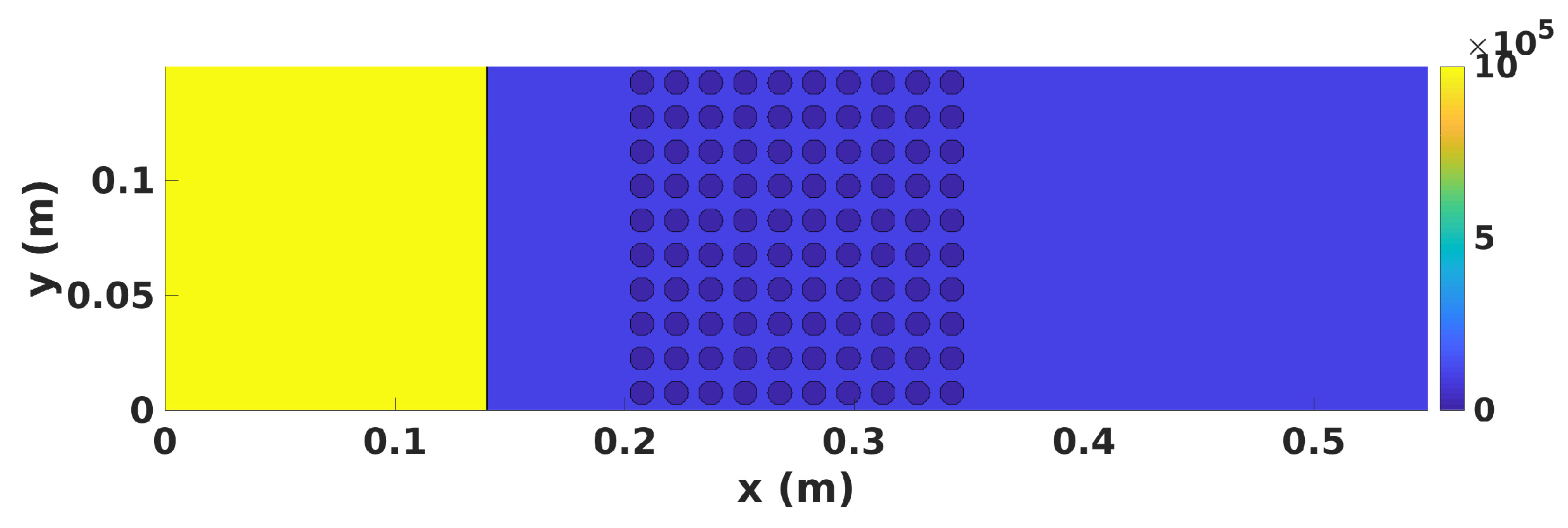
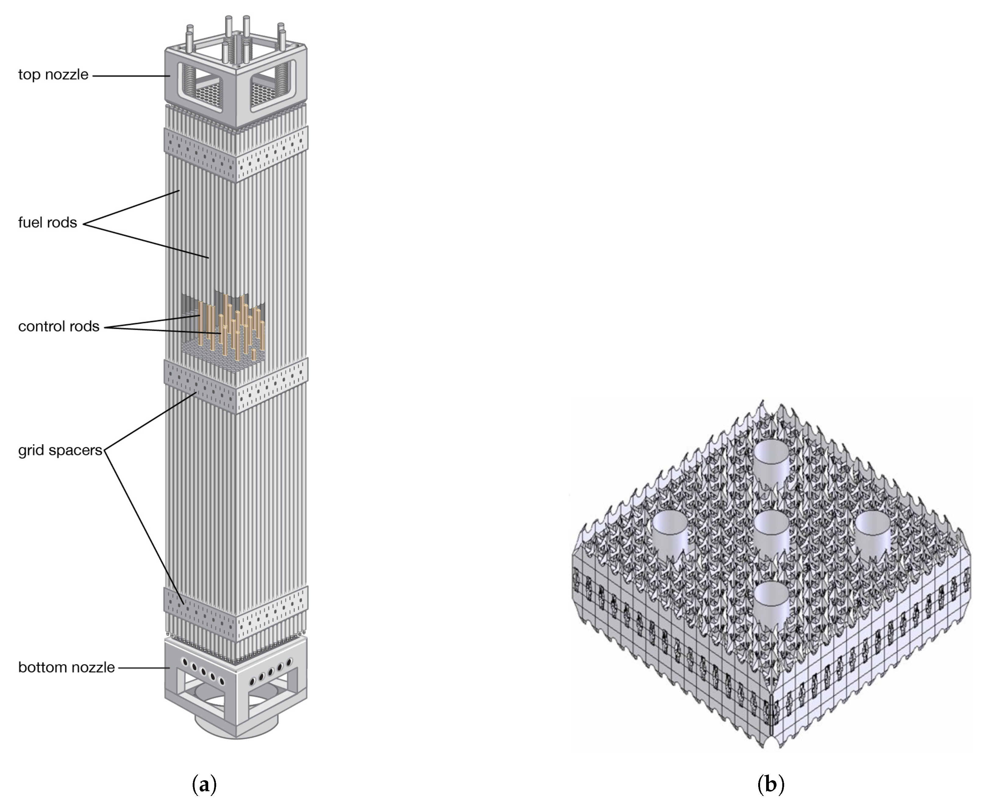
The simulation is designed as shown in Figure 3: a 2D transverse pressure wave propagates through a rod bundle composed of $10\times 10$ rods. As stated in the introduction, this test case can be seen as a simplified, yet representative, version of the actual pressure loading that would impact PWR fuel assemblies during a depressurization transient (known as loss of cooling accident, or LOCA).

Indeed, as can be seen in Figure 4, such a pressure wave would originate from a failure in one of the pipes of the primary loop and then propagate towards the main vessel. This initial plane wave is of course expected to undergo some diffraction at the junction between the 1D pipe and the 3D core. The first mechanical sollicitation on the fuel assemblies would then come from the transverse propagation of a (spherical) pressure wave, followed by a second vertical wave guided by the axial water flow. Thus, only the first wave is here considered, with a simplified modeling.

All the simulation parameters are specified in

Table 3. Geometry.

X-Dimension	Y-Dimension	Rods Radius	Distance between Consecutive Rods	Rods Position
$0.55\mathrm{m}$	$0.15\mathrm{m}$	$5\times {10}^{-3}\mathrm{m}$	$5\times {10}^{-3}\mathrm{m}$	$[0.2025\mathrm{m},0.3525\mathrm{m}]$

,

Table 4. Pressure loading.

10 Bar Pressure Zone	1 Bar Pressure Zone	Pressure Discontinuity ⟷ 1st Rod Bundles
$[0,0.14\mathrm{m}]$	$[0.14\mathrm{m},0.55\mathrm{m}]$	$6.75\times {10}^{-2}\mathrm{m}$

and

Table 5. Fluid parameters.

Reference Density	Reference Pressure	Sound Velocity
${\rho }_{ref}=1000\mathrm{k}\mathrm{g}·{\mathrm{m}}^{-3}$	$p_{ref}={10}^5\mathrm{Pa}$	$c=1300\mathrm{m}·{\mathrm{s}}^{-1}$

.

The fluid is considered compressible, inviscid and isothermal. It satisfies a barotropic state law:

$$p=p_{ref}+c^2(\rho -{\rho }_{ref}),$$

(13)

with the following numerical values.

As for the solid medium, the rods can here be considered as rigid bodies, whose centers are kinematically blocked, so that the sum of the reaction forces to the central blockages directly provides the force applied by the fluid to the microstructure.

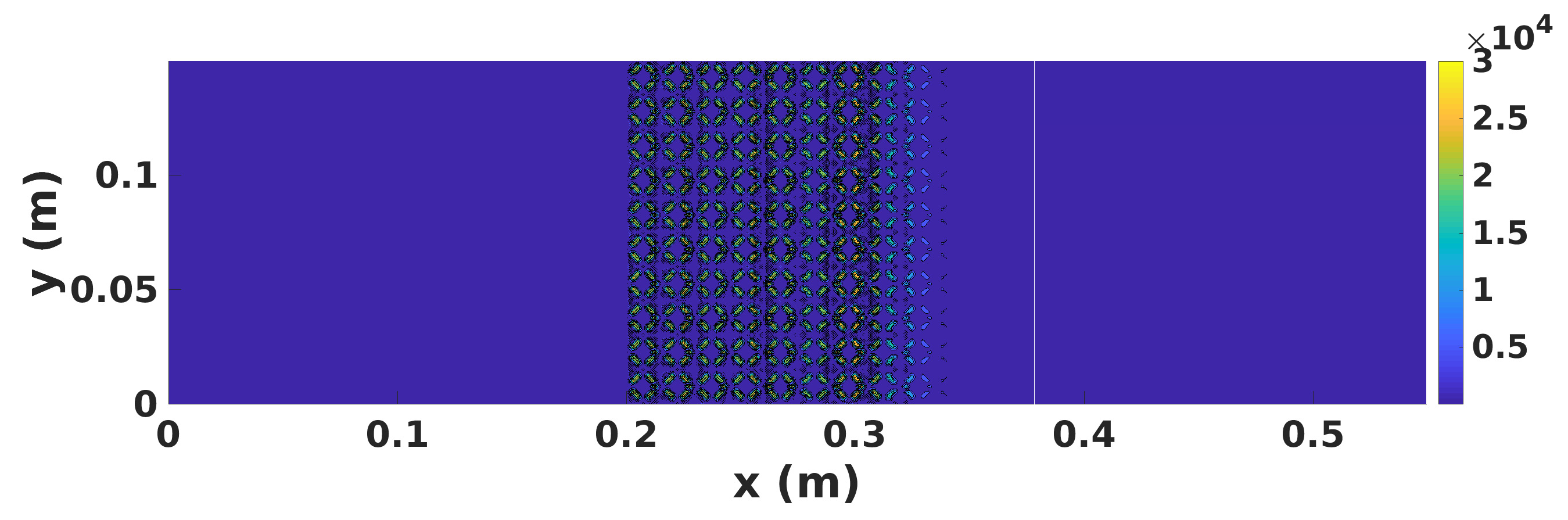
The mesh size is set to $\frac{r_b}{5}$, where $r_b=5\times {10}^{-3}\mathrm{m}$ is the rods’ radius. For the sake of convergence, finer mesh sizes of $\frac{r_b}{8}$, $\frac{r_b}{10}$ and $\frac{r_b}{12}$ are also computed. The spatial discretization of the equations is implemented through a finite element method for the solid medium (with 3-noded triangle elements), and a cell-centered finite volume scheme for the fluid (quadrangle elements, order 2 in time and space, HLL Riemann solver). An Euler explicit scheme is then used for the time discretization. 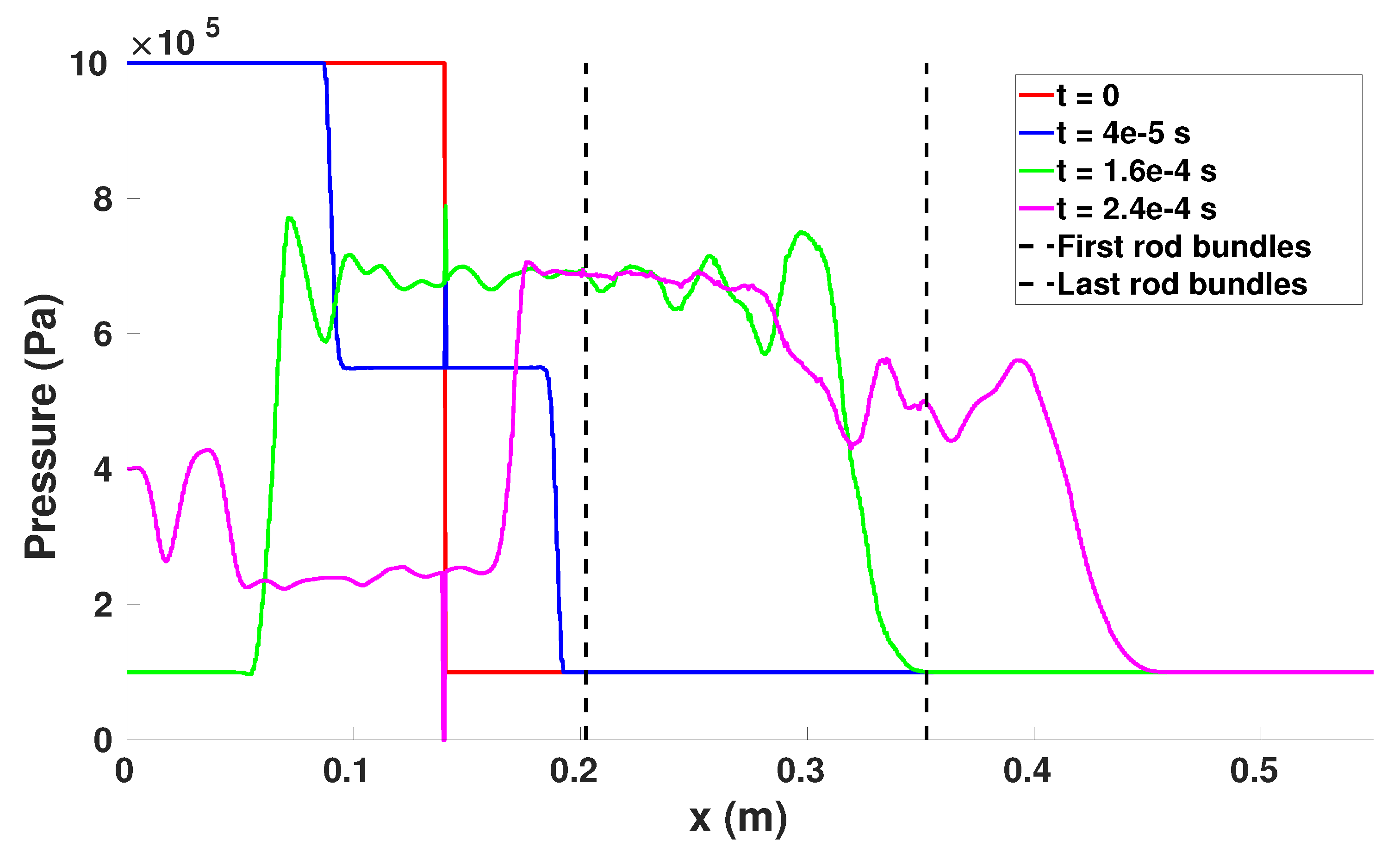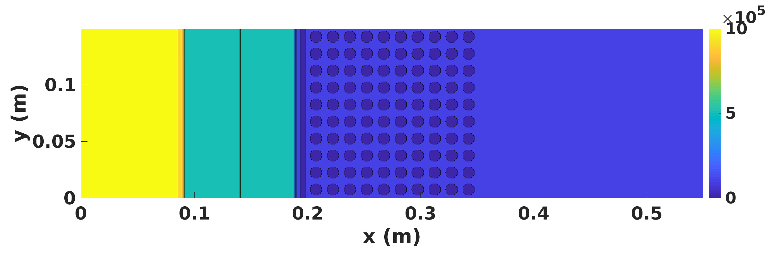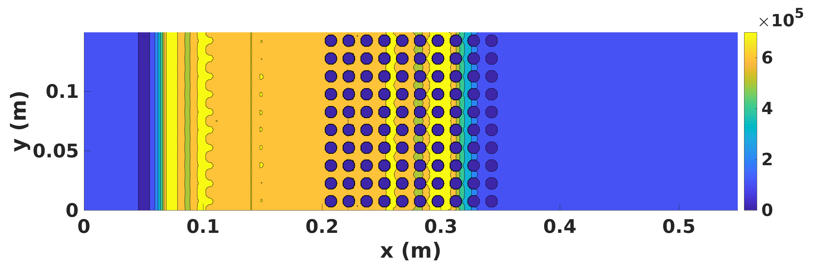The resulting pressure field is displayed in Figure 5, Figure 6, Figure 7 and Figure 8. It can be noted that, during the postprocessing, the pressure is by default set to zero on the nodes located outside the fluid domain.

As in a classical shock tube situation, the simulation shows two waves propagating in opposite directions from the initial discontinuity (Figure 5 at $t=4\times {10}^{-5}\mathrm{s}$, and Figure 6). The left one then bounces back on the left vertical boundary (defined with absorbing conditions) and heads back towards the solid medium (Figure 5, $t=1.6\times {10}^{-4}\mathrm{s}\mathrm{and}t=2.4\times {10}^{-4}\mathrm{s}$). This left boundary condition, not very familiar in shock tube computations or experiments, does not here affect the propagation of the pressure wave within the solid medium. Indeed, the simulation stops before the reflected wave hits back the solid medium. The same is true for the wave bouncing back on the right vertical boundary.

5.1. A Priori Accuracy Results

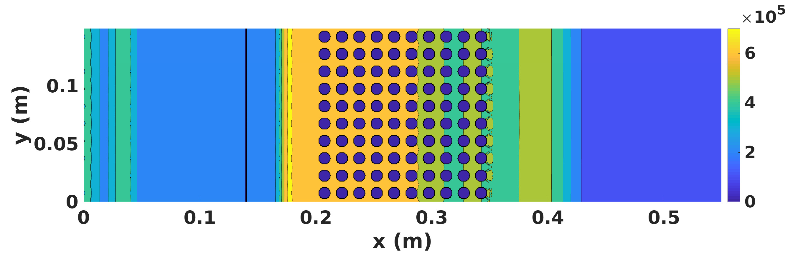
The reference solution being computed at the microscopic scale, the following wavelet postprocessing uses an interpolation of the pressure field on a 2D regular cartesian grid, whose mesh size equals $5·{10}^{-4}\mathrm{m}$, i.e., half the value of the reference computation grid. It is recalled that the pressure is by default set to zero on the nodes located outside the fluid domain. Given the microstructure geometry and reference pressure field (Figure 7), wavelengths around ${10}^{-3}\mathrm{m}$ and ${10}^{-4}\mathrm{m}$ are expected to convey a significant part of the pressure field information. In order to confront this estimation and determine both the relevant cutoff scale and the required number of wavelet coefficients, two accuracy criteria are hereafter introduced:

•

first, a criterion based on wavelets ability to preserve a signal $L^2$-energy:

$${∥f∥}_{L^2}^2=\frac{2\pi }{C_{\mathrm{\Psi }}}{\int }_0^{+\infty }{\int }_{{\mathbb{R}}^2}{\left|\mathcal{W}\left[f\right](s,\underline{u})\right|}^2\mathrm{d}\underline{u}\frac{\mathrm{d}s}{s^3},$$

(14)

which allows studying the impact of the number of wavelet coefficients $N_s$ on the $L^2$-energy recovery:

$$N_s⟼\frac{1}{{∥f∥}_{L^2}^2}\sum _{k=1}^{N_s}\frac{2\pi }{C_{\mathrm{\Psi }}}{∥\mathcal{W}\left[f\right](s_k,·)∥}_{L^2}^2\frac{\Delta s}{s_k^3},s_k\in \left[s_1,s_{N_s}\right];$$

(15)

•

second, a physics-driven criterion based on the force applied to the solid medium microstructure:

$$\underline{F_{F\to S}}\left(t\right)={\int }_{\partial {\Omega }_s}-p(\underline{\sigma },t){\underline{n}}_{S\to F}\left(\underline{\sigma }\right)\mathrm{d}\underline{\sigma },$$

(16)

which shall be compared to its approximation:

$${\left(\underline{F_{F\to S}}\right)}_{N_s}\left(t\right)={\int }_{\partial {\Omega }_s}-p_{N_s}(\underline{\sigma },t){\underline{n}}_{S\to F}\left(\underline{\sigma }\right)\mathrm{d}\underline{\sigma },$$

(17)

where $p_{N_s}$ is an approximation of the microscopic pressure field, obtained by computing the reconstruction formula (9) with $N_s$ scales on the range $[s_1,s_{N_s}]$.

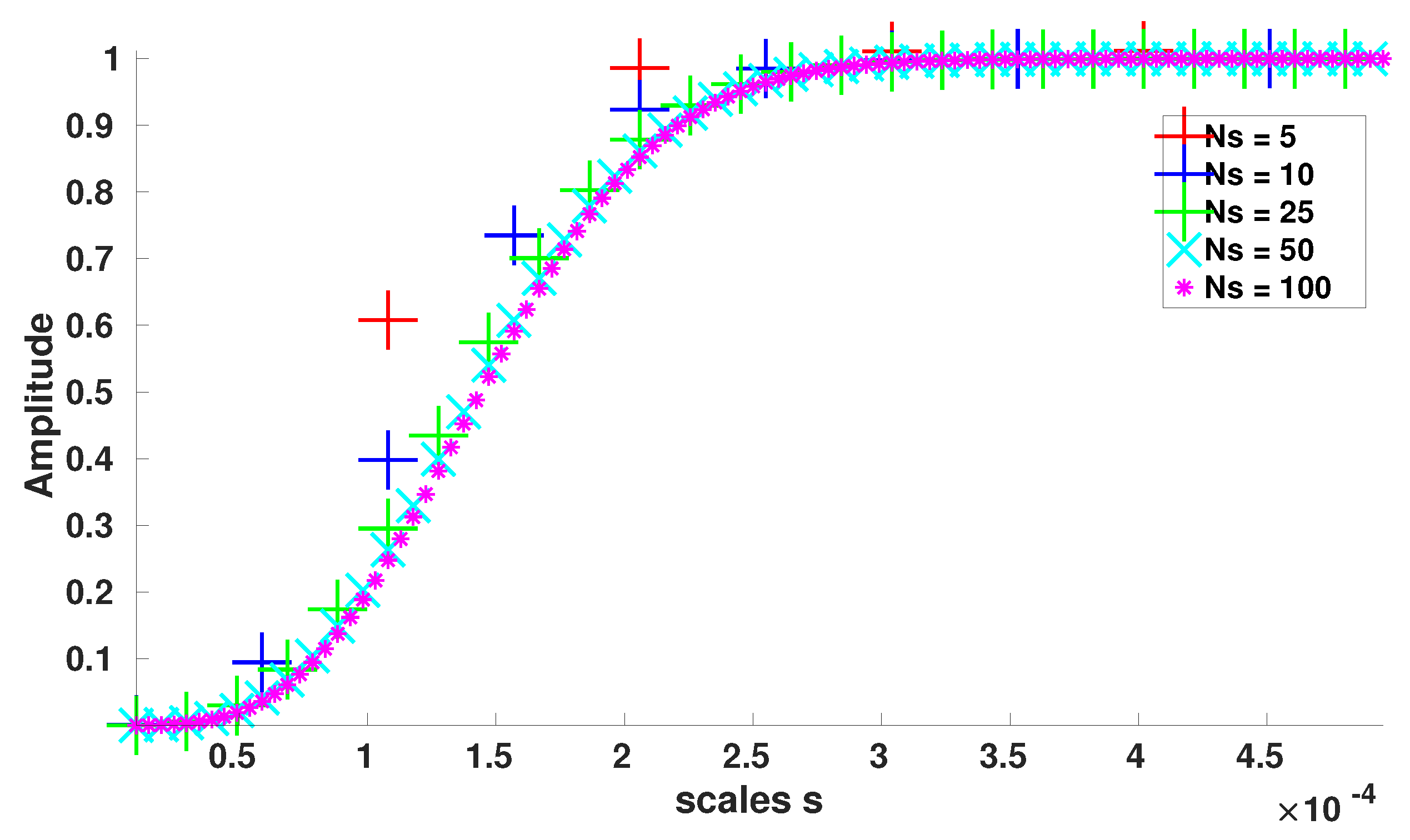
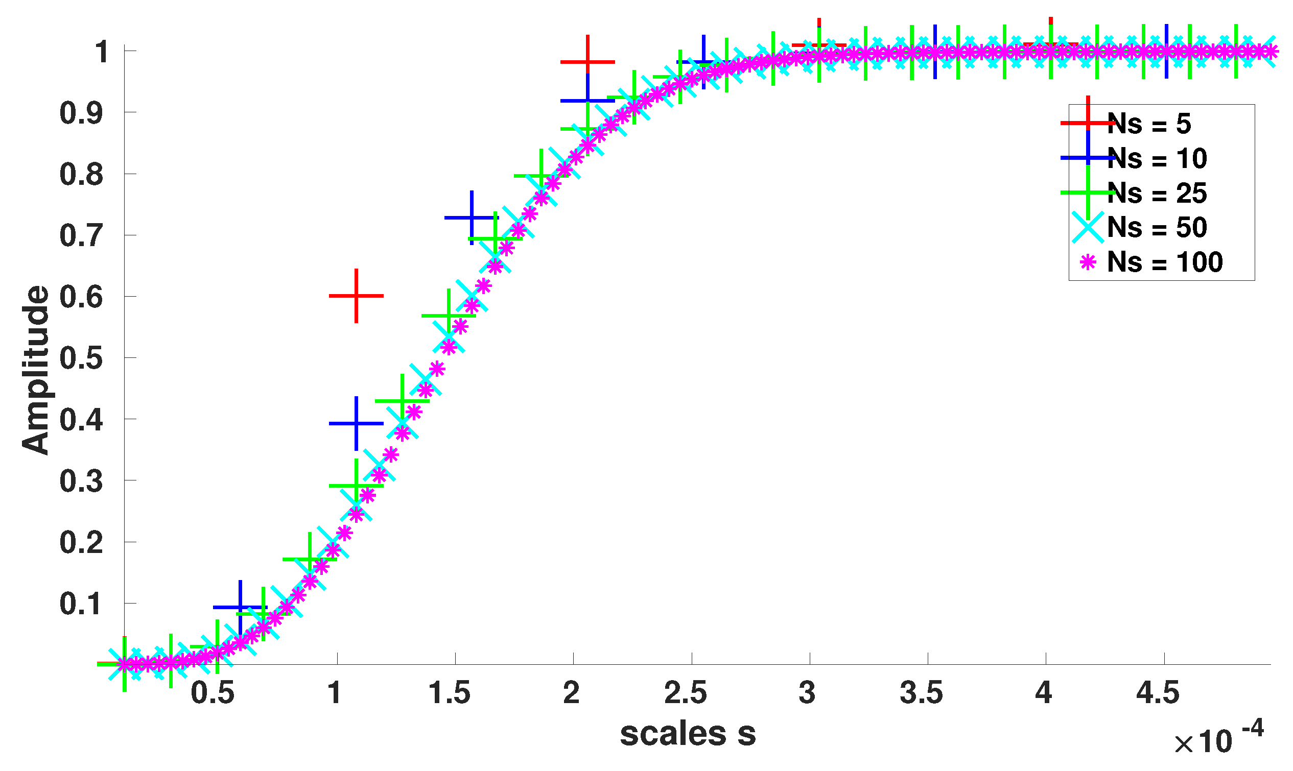
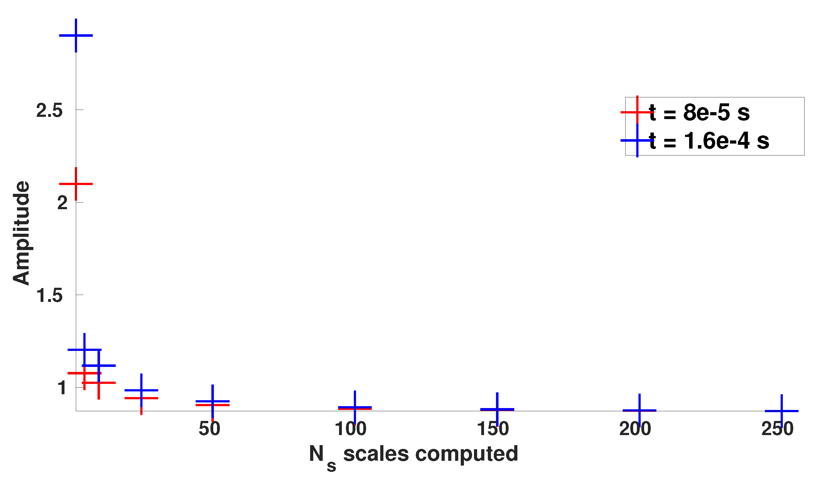
Starting with the $L^2$-energy criterion, Figure 9 and Figure 10 display, for two time instants for which the pressure discontinuity is located at different locations within the array of rods, the percentage of the reference pressure field $L^2$-energy that can be recovered with an increasing number of wavelet coefficients $\mathcal{W}\left[p\right](s,·)$, on the scale range $s\in [{10}^{-5},5\times {10}^{-4}]$.

Thus, it appears that for the two different time instants, the scale range $s\in [{10}^{-5},5\times {10}^{-4}]$, which theoretically corresponds to wavelengths starting from $\lambda \in [2.4\times {10}^{-5},6.5\times {10}^{-5}\mathrm{m}]$ up to $\lambda \in [1.2\times {10}^{-3}\mathrm{m},3.3\times {10}^{-3}\mathrm{m}]$, conveys around $100\%$ of the pressure field $L^2$-energy. Thus, regardless of the location of the pressure discontinuity within the array of rods, the most energetic scales seem to be invariant and constrained by the microstructure geometry.

Nevertheless, it could seem surprising to detect “wavelengths” smaller than the grid mesh size $(5\times {10}^{-4}\mathrm{m})$. However, it is here important to highlight the fact that the scale parameter does not only drive the wavelets bandwidth (and thus the “observable” wavelengths), but also the amplitude of the wavelet coefficients, as can be seen in Equation (6). Thus, by decreasing the scale parameter, it is possible to increase the value of the homogenized density and pressure variables in the vicinity of the solid medium microstructure and thus better represent the fact that the fluid shall not penetrate the solid medium. Therefore, the smallest scales detected in Figure 9 and Figure 10 are not connected to actual and physical wavelengths. Conversely, it can be outlined that wavelet coefficients $\mathcal{W}\left[p\right](s,·)$ with $s\ge {10}^{-4}$, which gather around $80\%$ of the pressure $L^2$-energy, are connected to (actual) wavelengths wider than the grid mesh size ${5.10}^{-4}\mathrm{m}$$\left(\lambda \in [2.4\times {10}^{-4},6.5\times {10}^{-4}\mathrm{m}]\mathrm{for}s={10}^{-4}\right)$.

Finally, it can be noted that a decrease in the number of computed coefficients $N_s$ does not have a significant impact on the $L^2$-energy recovery. Indeed, the asymptotic value still reaches around $100\%$, even with only five wavelet coefficients.

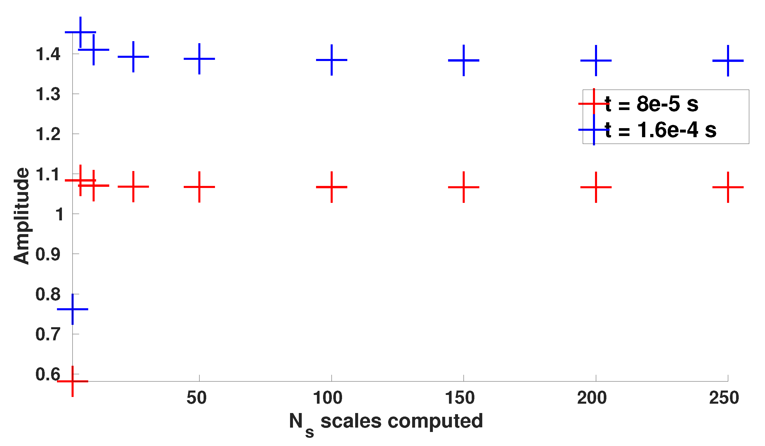
Let us now turn towards the second criterion in order to check whether similar conclusions are reached. Figure 11, Figure 12 and Figure 13 show the evolution of the force ratio, evaluated on the whole microstructure, with the number of computed scales $N_s$, and for three different scale ranges: $s\in [{10}^{-5},5\times {10}^{-4}]$, $s\in [{10}^{-5},{10}^{-3}]$, and $s\in [{10}^{-4},{10}^{-3}]$. It is recalled that the force ratio is defined by:

$$N_s⟼\frac{{\left(\underline{F_{F\to S}}\right)}_{N_s}·\underline{e_x}}{\underline{F_{F\to S}}·\underline{e_x}},$$

(18)

where $\underline{F_{F\to S}}$ and ${\left(\underline{F_{F\to S}}\right)}_{N_s}$ are defined in Equations (16) and (17), and $\underline{e_x}$ is a unit horizontal vector, heading from left to right.

Conversely to the $L^2$-energy criterion, the scale range $s\in [{10}^{-5},5\times {10}^{-4}]$ seems here unsuited to properly reconstruct the force applied to the solid medium microstructure, as an almost $40\%$ overestimation can be witnessed for the time instant $t=1.6\times {10}^{-4}\mathrm{s}$. Furthermore, an $8\%$ overestimation is still visible for the time instant $t=8\times {10}^{-5}\mathrm{s}$. This significant difference between the two time instants can be explained by the following fact: as the initial pressure wave has almost exited the array of rods for $t=1.6\times {10}^{-4}\mathrm{s}$ (see Figure 7), wavelengths around $5\times {10}^{-3}\mathrm{m}$ (driven by the rods radius), which are not taken into account in the scale range $s\in [{10}^{-5},5\times {10}^{-4}]$, are much more present within the solid medium microstructure than for the time instant $t=8\times {10}^{-5}\mathrm{s}$.

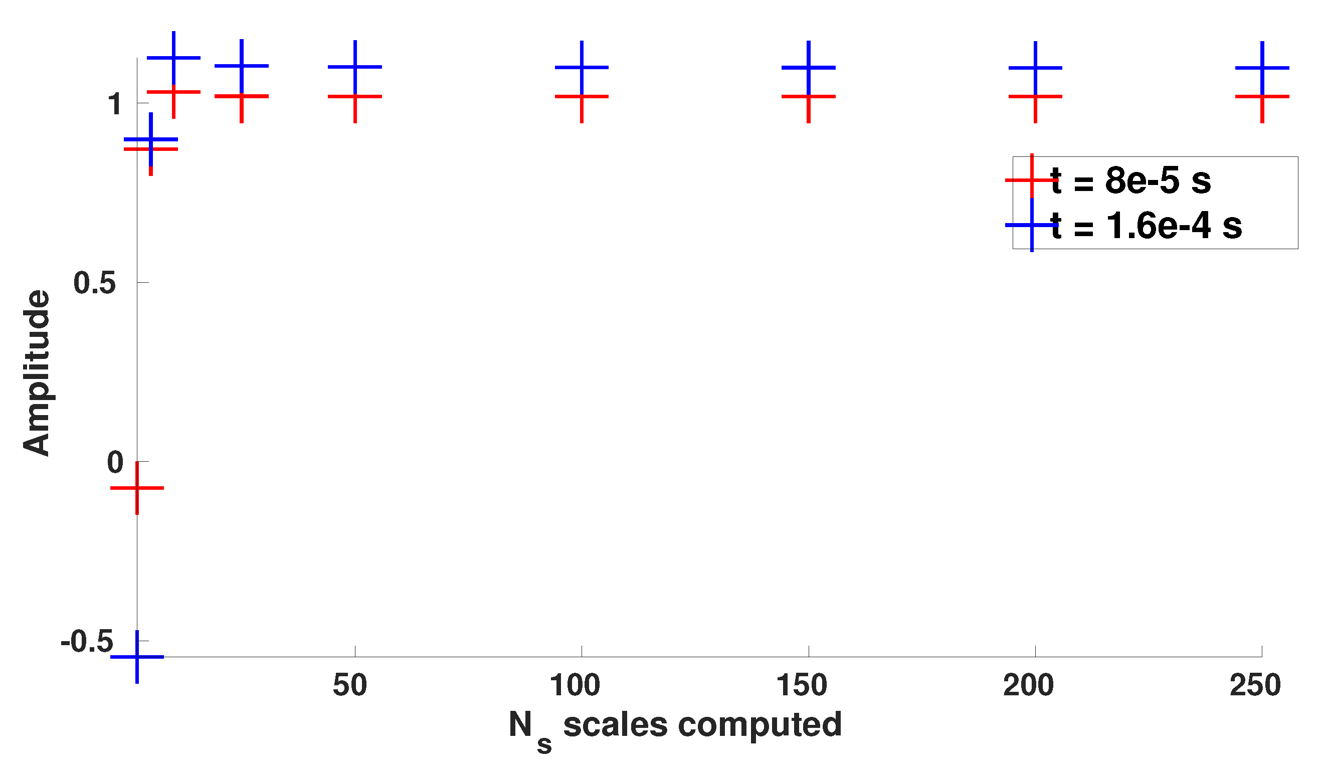
Thus, the wider scale range $s\in [{10}^{-5},{10}^{-3}]$ allows to better reconstruct the force for both time instants, with, for instance, an overestimation around $10\%$ for $t=1.6\times {10}^{-4}\mathrm{s}$. Additionally, Figure 13 proves that the smallest scales could even be neglected without losing accuracy, thus leading to the range $s\in [{10}^{-4},{10}^{-3}]$, which contains wavelengths $\lambda \in [2.4\times {10}^{-4},6.5\times {10}^{-3}\mathrm{m}]$. This is a very interesting result in the perspective of building a filtered solver for the fluid equations, since it will allow a coarser and thus more efficient discretization at macroscale while preserving the quantity of interest at microscale for the interaction with the structure.

Finally, it can be noticed that $N_s=10$ wavelet coefficients would already allow reaching a good accuracy $\left(\le 10\%\mathrm{overestimation}\right)$ on the force applied to the solid medium microstructure. The results and recommendations for the most efficient filtering obtained with this physics-driven criterion are thus summarized in

Table 6. Cutoff scale and number of wavelet coefficients.

Cutoff Scale and Number of Wavelet Coefficients
$s_{min}={10}^{-4}$	$N_s=10$	$s_{max}={10}^{-3}$
$\lambda \in \left[2.4\times {10}^{-4},6.5\times {10}^{-4}\mathrm{m}\right]$		$\lambda \in \left[4.8\times {10}^{-4},1.3\times {10}^{-3}\mathrm{m}\right]$

.

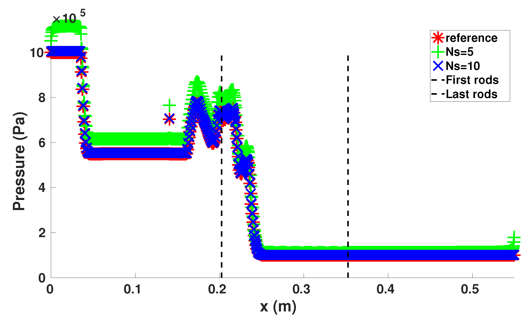
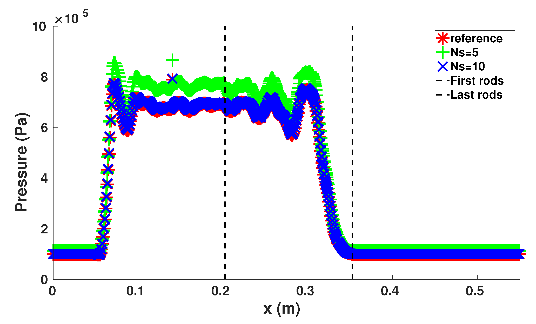
For the sake of completeness, Figure 14 and Figure 15 display the reference and reconstructed pressure fields along the medium horizontal axis, while Figure 16 and Figure 17 display the absolute error between the 2D reference and reconstructed pressure fields. The absolute error is logically located in the vicinity of the rods, where the reference pressure variations are maximal, but it remains small compared to the reference pressure range (less than 10% for maximum values). Furthermore, the good results obtained in terms of forces acting on the structure indicate that the pressure gradient is well preserved.

5.2. Short Summary of the Main Results

To summarize the results regarding the implementation of the CWT filtering technique to a representative unsteady pressure field, it can be emphasized that the use of continuous wavelet transform, with the isotropic Mexican hat as the analyzing wavelet, allowed, on the one hand, selecting the most relevant wavelengths within the reference field and, on the other hand, reconstructing, with a small number of homogenized coefficients and a very good accuracy, the force applied to the solid medium microstructure.

These results demonstrate the promising expected properties of the proposed approximation approach for the construction of a homogenized representation of the fluid problem in the section of fuel assembly crossed by pressure waves. Moreover, it is important to quote that the results were obtained above in the most selective case of a stiff shock propagating through the rod bundle. In a situation closer to the addressed physics where the pressure signal coming from a partially diffracted rarefaction wave is much smoother, the scale selection is likely to be even more efficient, and with it, the computational performance of an associated macroscale solver for the filtered fluid equations.

6. Conclusions

A new homogenization formalism, based on continuous wavelet transform, was introduced. Its application on a local pressure field obtained numerically showed its ability to construct a homogenized representation of the pressure field, and thus of the fluid forces acting on the structure. It can moreover be noticed that this new filtering process is independent from the microstructure periodicity or shape.

The accuracy results were highlighted through a comparison of the filtered pressure field to a reference solution corresponding to the representative case of a transverse pressure wave propagating through the cross section of a 10 × 10 array of rods. The isotropic Mexican hat wavelet allowed determining a relevant cutoff scale, and the number of wavelet coefficients necessary to reach a good accuracy on the force applied to the solid medium microstructure.

This result is a key component towards the design of a coupled fluid-structure solver implementing the proposed approximation of the fluid physical fields for compressible pressure waves. Indeed, the proposed homogenization formalism, based on continuous wavelet transform, will allow to robustly derive filtered equations governing a homogenized fluid, while taking properly into account boundary conditions, and connecting resolved and unresolved scales without any ad hoc model for the closure expression. In further developments, the focus shall thus be put on the direct computation of the filtered fluid equations. Following this work, both the deformation and displacement of the solid medium will be taken into account, for instance, by introducing equivalent springs.