Article

A Theoretical Model of Long Rossby Waves in the Southern Ocean and Their Interaction with Bottom Topography

by
David P. Marshall
Department of Physics, University of Oxford, Oxford OX1 3PU, UK
Fluids 2016, 1(2), 17; https://doi.org/10.3390/fluids1020017
Submission received: 25 April 2016 / Revised: 19 May 2016 / Accepted: 24 May 2016 / Published: 27 May 2016
(This article belongs to the Collection Geophysical Fluid Dynamics)

Abstract

:
An analytical model of long Rossby waves is developed for a continuously-stratified, planetary geostrophic ocean in the presence of arbitrary bottom topography under the assumption that the potential vorticity is a linear function of buoyancy. The remaining dynamics are controlled by equations for material conservation of buoyancy along the sea surface and the sea floor. The mean, steady-state surface circulation follows characteristics that are intermediate to f and f / H contours, where f is the Coriolis parameter and H is the ocean depth; for realistic stratification and weak bottom currents, these characteristics are mostly zonal with weak deflections over the major topographic features. Equations are derived for linear long Rossby waves about this mean state. These are qualitatively similar to the long Rossby wave equations for a two-layer ocean, linearised about a state of rest, except that the surface characteristics in the wave equation, which dominate the propagation, follow precisely the same path as the mean surface flow. In addition to this topographic steering, it is shown that a weighted integral of the Rossby propagation term vanishes over any area enclosed by an f / H contour, which has been shown in the two-layer model to lead to Rossby waves “jumping” across the f / H contour. Finally, a nonlinear Rossby wave equation is derived as a specialisation of the result previously obtained by Rick Salmon. This consists of intrinsic westward propagation at the classical long Rossby speed, modified to account for the finite ocean depth, and a Doppler shift by the depth-mean flow. The latter dominates within the Antarctic Circumpolar Current, consistent with observed eastward propagation of sea surface height anomalies.

Graphical Abstract

1. Introduction

The fluid dynamics of the Southern Ocean is distinct from other ocean basins in a number of key respects. Firstly, unimpeded by continental barriers, the Antarctic Circumpolar Current (ACC) is the only ocean current to circumnavigate the globe. Moreover, since the input of momentum from the surface wind stress is mostly balanced by the transfer of momentum to the solid Earth by a bottom form stress [1], the ACC extends all the way down to the sea floor; yet, despite navigating a complex topographic domain, the ACC follows a remarkably zonal path with only weak steering of the upper level circulation by the bottom topography. Furthermore, whereas surface anomalies propagate westward at virtually all latitudes [2,3], within the ACC surface, anomalies propagate eastward relative to the sea floor [4,5,6]. While the vast majority of these observed surface anomalies are admittedly nonlinear eddies, as opposed to linear long Rossby waves, Chelton et al. [2] and Chelton et al. [3] find that these nonlinear eddies propagate westward at roughly the long Rossby wave speed at mid-latitudes. Klocker and Marshall [6] show that the eastward propagation of anomalies within the ACC is consistent with the long Rossby wave speed if the latter includes a Doppler shift by the depth-mean flow.
Traditionally, the impact of bottom topography on the depth-integrated circulation has been described through the JEBAR (“Joint Effect of Baroclinicity and Relief”) mechanism [7,8]. However, JEBAR can greatly exaggerate the topographic forcing, for example predicting large impact of topography even on a surface-confined current in which the abyssal velocities vanish [9]. Instead, Marshall [10], Marshall [11], and Marshall and Stephens [12] (see also [13]) formulate a model of topographic steering in which bottom topography affects the circulation in compensating ways. Firstly, the vertical velocities at the sea floor, generated as fluid parcels, move up and down the bottom slope, compressing and stretching the vortex tubes above. However, this vertical motion also advects the buoyancy field, creating lateral buoyancy gradients throughout the fluid column which indirectly modify the vorticity balance by creating a depth-integrated lateral advection of planetary vorticity. For realistic oceanographic parameters, it turns out that this latter process is dominant, having the effect of greatly reducing the net topographic impact.
For steady-state flow at low Rossby number, de Szoeke [14], Marshall [10] and Marshall [11] have shown that the circulation is determined by a characteristic problem in which the “characteristics”, corresponding to the surface streamlines in the absence of forcing, are intermediate to f contours and f / H contours, where f = 2 Ω sin ϕ is the Coriolis parameter, Ω is the angular velocity of rotation of the Earth and ϕ is latitude, and H is the ocean depth. The limiting cases of the characteristics being dominated by f and f / H contours correspond to a surface-intensified, baroclinic circulation and depth-independent barotropic circulation, respectively. This leads to the natural definition of “topographic steering” of the mean flow as the extent to which these characteristics are deformed by the bottom topography from latitude circles. This topographic steering depends on both the stratification and strength of the bottom currents. However, for time-dependent flow, the concept of topographic steering is, a priori, less obvious.
In this manuscript, an analytical model is developed for long Rossby waves in the Southern Ocean in the presence of both background flow and arbitrary variations in bottom topography by extending the mathematical approach of Marshall [11] for the steady problem to include time-dependence. The resultant model represents a specialisation of the more general approach of Salmon [15] who derived equations for low Rossby number flow under an assumption of a functional relation between the potential vorticity and buoyancy. Specifically, it is shown that:
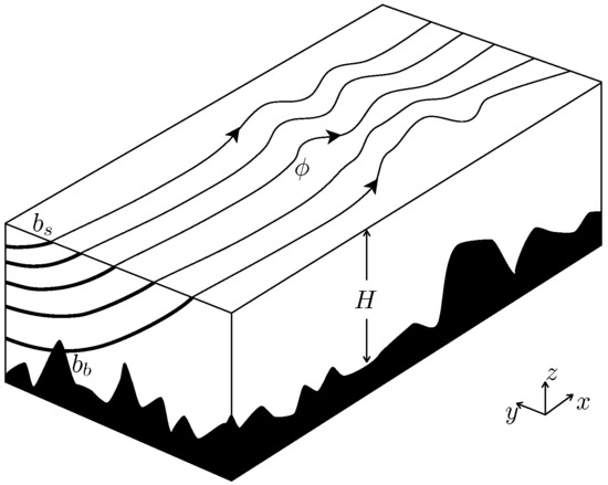
  • Long Rossby waves are “steered” by the bottom topography in precisely the same manner as the time-mean surface streamlines. In the limit in which the surface flow is relatively unaffected by the bottom topography, so are the long Rossby waves. This concept is made rigorous through comparison of the mathematical equations for long Rossby waves in the present continuously-stratified model with variable bottom topography and the the equivalent equations for long Rossby waves in a two-layer model, linearised about a state of rest.
  • The result that long Rossby waves propagate quasi-zonally breaks down catastrophically wherever f / H contours close, irrespective of the stratification. This is demonstrated through the derivation of an integral constraint in which a weighted integral of the dominant Rossby propagation term vanishes over any area enclosed by an f / H contour. Such behaviour has been studied in the analogous two-layer model [16] and has been shown to result in the long Rossby waves partially “jumping” across the closed f / H contour.
  • Following the approach of Salmon [15], a nonlinear long Rossby wave equation can be derived which demonstrates, in this model, that the long Rossby wave speed is Doppler shifted by the depth-mean flow. For realistic ACC parameters, the latter term dominates and causes eastward propagation relative to the sea floor, at speeds consistent with the observed eastward propagation of Southern Ocean surface anomalies.
The manuscript is organised as follows. In Section 2, the planetary geostrophic equations are stated, along with the kinematic boundary conditions and the general steady-state solution. In Section 3, these equations are applied to the Southern Ocean through the ansatz of the potential vorticity being a linear function of the buoyancy. In Section 4, the mean, steady-state solution is reviewed. In Section 5, the equations for linear long Rossby waves about the mean state are derived, related to the two-layer model to identify explicitly how long Rossby waves are “steered” by the bottom topography. Moreover, it is demonstrated that bottom topography still has a major impact whenever the f / H contours close through an integral constraint, leading to the long Rossby waves partially “jumping” across these closed contours. In Section 6, the nonlinear long Rossby wave equation is derived following the approach of Salmon [15] to establish that the long Rossby waves are Doppler-shifted by the depth-mean flow. Concluding remarks are made in Section 7.

2. Planetary Geostrophic Equations

We consider unforced, planetary geostrophic flow [17] between two rigid boundaries located at the sea surface, z = 0 , and sea floor, z = H ( x , y ) , as sketched in Figure 1. The equations of motion are thus:
f k × u + p ρ 0 = 0 ,
b + 1 ρ 0 p z = 0 ,
· u + w z = 0 ,
b t + u · b + w b z = 0 .
Here, u and w are the horizontal and vertical components of the velocity, f = f ( y ) is the Coriolis parameter that varies with latitude, and p is pressure. ρ 0 is the reference density and b is buoyancy. For simplicity, we adopt a Cartesian coordinate system ( x , y , z ) where x is the zonal, y the meridional and z the vertical coordinate, and t is time. Note that compressibility effects are not taken into account. Boundary conditions are no normal flow at the sea floor and sea surface:
w = 0 ( z = 0 ) ,
w = u · H ( z = H ) .
These equations hold only in the limit of a very small Rossby number, Ro = U / f L 1 , where U and L are characteristic velocity and length scales e.g., [18]. Thus, for consistency, it is necessary for the bottom topography to vary only on planetary scales, which is generally not the case in the ocean. Furthermore, the model may spontaneously generate smaller scales of motion that invalidate the planetary geostrophic dynamics through instabilities [19] or through interactions with the bottom topography (of which the mechanism discussed in [16] and Section 5.3 of this manuscript is a good example).
The general steady-state solution to these planetary geostrophic equations can be written [20]:
Q = Q ( M , b ) ,
where
Q = f b z
is the potential vorticity, and
M = p ρ 0 b z
is the Montgomery potential (the planetary geostrophic approximation to the Bernoulli potential). It is easily shown that the flow materially conserves each of Q, M and b in the steady state [20]. Likewise, in the steady state, the boundary conditions can be rewritten as:
M s = M s ( b s ) ,
M b = M b ( b b ) ,
where the subscripts s and b are introduced for the surface and bottom boundaries, respectively [11].

3. Application to the Southern Ocean

We now describe the specific application of the planetary geostrophic equations to the Southern Ocean. The following represents the extension of Marshall [11] to include time dependence.

3.1. Interior Dynamics

The basic concept underlying the present model is to focus on the dynamical influence of the surface and bottom boundaries. In this spirit, we exclude any interesting interior dynamics, a priori, by imposing the ansatz of uniform potential vorticity on density surfaces, which renders the solution for the evolution interior potential vorticity field trivial. Salmon [15], Marshall [10], Marshall and Stephens [12] discuss steady solutions for more general functional relations between the potential vorticity and density, but here we restrict our attention to the analytically simpler scenario of a linear relation,
Q = f b z = a b ,
giving an exponential variation of buoyancy with depth:
b = b s e a z / f .
Marshall [11] used the value a = 6.44 × 10 8 m 1 s 1 estimated by Marshall et al. [21] from a logarithmic fit to potential density observations, giving an e-folding scale for the stratification of about 1600 m . However, a more recent analysis by Kartsen and Marshall [22] finds that the e-folding scale varies across the ACC between about 500 m on its southern flank and 1500 m on its northern flank, with a mean value of about 1000 m . These variations in e-folding depth provide some indication of the limitations of the ansatz Equation (12). Taking f 10 4 s within ACC, we obtain the value a = 10 7 m 1 · s 1 , slightly larger than used in [11]; however, this different choice has minimal qualitative impact on the solutions.
Setting z = H provides a relation between the surface and bottom densities,
b b = b s e a H / f ,
and hence it is sufficient to determine the solution for either b s or b b since only one is independent in this model. We also have, through hydrostatic balance (Equation (2)) and the functional form of the potential vorticity (Equation (12)):
1 ρ 0 p z = f a b z .
Integrating vertically and using Equation (9) gives
M b = M s γ b s ,
where
γ = f a 1 e a H / f a H f e a H / f
depends purely on the bottom depth, H ( x , y ) , the Coriolis parameter, f ( y ) , and the prescribed constant a that sets the e-folding depth of the stratification.

3.2. Boundary Conditions

At the surface and bottom boundaries, material conservation of buoyancy equation (4) can be rewritten:
b s t + u s · b s = 0 ,
b b t + u b · b b = 0 .
Noting that
u s = 1 f k × M s ,
since M s = p s / ρ 0 , and
u b = 1 f k × M b H f k × b b ,
(see Appendix A in [10]), we obtain:
b s t + 1 f J M s , b s = 0 ,
b b t + 1 f J M b , b b = 0 .
Here, the Jacobian operator is defined:
J ( a , b ) = a x b y a y b x .
Through Equation (14), only one of the time derivatives in Equations (22) and (23) is independent, resulting in the balance condition:
e a H / f J M s , b s = J M b , b b .
Substituting for b b and M b using Equations (14) and (16), we find, after some algebra,
J ( γ , b s ) = J a H f , M b = J a H f , M s γ b s .
This relation Equation (25), which is equivalent to a depth-integrated linear vorticity balance, couples variations in surface density along γ contours to M b variations along f / H contours. With some caveats that we shall discuss in Section 5.3, Equations (22) and (25) provide a complete description of the temporal evolution of the surface fields, b s and M s , and thence for the three-dimensional circulation. Equations (22) and (25) are necessarily equivalent to (2.17) and (2.19) in Salmon [15] in the specialised limit of a linear relation between potential vorticity and buoyancy.

4. Steady State

4.1. Characteristics

In the steady state, Equations (22) and (23) indicate that the Montgomery potential and density contours are coincident at the upper and lower boundaries. Following Marshall [11], we assume a linear functional relation at the sea floor,
M ¯ b = H ref b ¯ b ,
where H ref is the “reference depth” [10]. This linear relation allows for analytical solution of the problem at the expense of some generality. The bottom velocity Equation (21) becomes
u ¯ b = ( H H ref ) f k × b ¯ b .
Thus, the reference depth has a simple physical interpretation as that at which the fluid velocity vanishes along the sea floor. Note that this concept is different to the more general “level of no motion”, frequently encountered in physical oceanography, in the sense that the flow vanishes at the reference depth only along the sea floor but not in the ocean interior.
Now substituting Equation (26) in Equation (16), we find
M ¯ s = γ + H ref e a H / f b ¯ s = ϕ b ¯ s ,
where
ϕ = γ + H ref e a H / f = f a 1 e a H / f a ( H H ref ) f e a H / f .
Since both b s and M s are materially conserved by fluid parcels in the steady state, the surface flow follows contours of ϕ , as sketched schematically in Figure 1:
b ¯ s = b ¯ s ( ϕ ) ,
M ¯ s = M ¯ s ( ϕ ) .
Contours of ϕ are the characteristics for the more general steady-state problem with wind forcing (Marshall, 1995a). Note that these characteristics, and hence the path of the surface current, depend only on the bottom depth, the Coriolis parameter, and the prescribed constants, a and H ref .
Plotted in Figure 2 are contours of f / H , γ (Equation (17)), and ϕ for H r e f = 4 km and 6 km . Note that the characteristic contours, ϕ , are quasi-zonal for these parameter choices, with only slight deflections over the major topographic, in marked contrast to both f / H and γ. The Kerguelen Plateau (between about 65 70 E, in the Indian sector) is notable in representing a more substantial topographic obstacle.

4.2. An Illustrative Solution

In order to construct the full solution, it is necessary to construct a mapping between the characteristic function, ϕ , and the surface buoyancy, b ¯ s . Several such examples are discussed in Marshall [11]; here, a single example is presented to provide the reader with an illustration of the key features, strengths and limitations of the model solutions. Specifically, the solution is constructed with the reference depth, H r e f = 4 km ; the surface buoyancy is set to a uniform constant value of 0.2 × 10 2 m · s 2 poleward of the ϕ = 1250 m contour (located around 60S), then it increases linearly with ϕ across the model ACC until ϕ = 1150 m (located around 52N), north of which the surface buoyancy is held constant.
Thereafter, the full solution can be constructed. The vertical structure of the pressure field is obtained by using Equation (15), alongside Equations (9) and (28), to give:
p ¯ ρ 0 = M ¯ s f b ¯ s a 1 e a z / f = f b ¯ s a e a z / f e a H / f a ( H H r e f ) f e a H / f .
Having obtained the vertical structure of the flow, the streamfunction for the depth-integrated flow can be shown to be:
ψ ¯ = b ¯ s a 2 ϕ H r e f e a H / f a H f ( H H r e f ) e a H / f ϕ ( b ¯ s ) a d b ¯ s
(see Appendix A). The reader is also referred to [11] for further details.
A three-dimensional perspective of the surface buoyancy field and a vertical section through the solution at the longitude of 150 W is shown in Figure 3, and the streamfunction for the depth-integrated flow is plotted, along with the pressure, or geostrophic streamlines, at depths of 0 km , 2 km and 4 km , and these are shown in Figure 4. By construction, the surface buoyancy contours, b ¯ s , and surface pressure contours, p ¯ s / ρ 0 = M ¯ s , follow the surface characteristic contours, ϕ .
The flow is quasi-zonal over most of the water column with only modest excursions over the topographic features. The two most obvious exceptions are in the Drake Passage where most, but not all, of the streamlines are able to pass through the passage, and the Kerguelan Plateau, which acts as a complete barrier to the modelled ACC. In reality, the ACC flows several degrees further north in the Indian sector and hence is able to skirt the northern tip of the Kerguelan Plateau. The latter is a limitation of the present model which lacks the necessary dynamics to allow the current to deflect northward after passing through the Drake Passage and return poleward as it passes around Antarctica. Traditionally, the latter has been assumed to be a consequence of Sverdrup balance following Stommel [23], although more recent work points to an important role for mesoscale eddies in controlling these meridional excursions [24].
The circulation is strongly surface-intensified, but nevetheless roughly equivalent barotropic over the upper 3 km of the water column, consistent with the theoretical arguments of Killworth [25]. In contrast, at 4 km depth, the flow consists of local abyssal recirculation gyres, confined by the bottom topography. Indeed, it is easily confirmed, by substituting z = H = H r e f in Equation (32), that the pressure is constant along the reference depth contour on the sea floor, i.e., the contour H = H r e f is a geostrophic streamline.
In summary, the time-mean solution has both strengths and weaknesses. The most significant virtue of the model is that it provides a continuously stratified solution to the planetary geostrophic equations that satisfies the kinematic boundary conditions at the sea surface and sea floor. However, the underlying assumptions, including uniform potential vorticity on buoyancy surfaces and the neglect of forcing by surface winds and mesoscale eddies, limit its broader applicability. Also note that some of the flow features formed within the solution are at odds with the low Rossby number assumption required for validity of the model. Nevertheless, the model provides a nice theoretical laboratory within which to investigate the behaviour of long Rossby waves in the presence of variable bottom topography.

5. Linear Rossby Waves

5.1. Linear Wave Equations

We now seek wave solutions, linearised about the steady state solution reviewed in Section 4. The linearised surface buoyancy equation (22) is:
b s t + 1 f J M ¯ s , b s + 1 f J M s , b ¯ s = 0 .
Using Equations (16) and (28), this can be rewritten:
b s t + 1 f J ϕ b ¯ s , b s 1 f J b ¯ s , γ b s 1 f J b ¯ s , M b = 0 .
Finally, using the relation
J b ¯ s , γ b s = ϕ J b ¯ s , b s J b ¯ s , H ref b b ,
which follows from Equations (29), (30) and (14), the linear long Rossby wave equation is:
b s t + b ¯ s f J ϕ , b s 1 f J b ¯ s , M b H ref b b = 0 .
In addition, we have the linearized version of Equation (25) as a constraint:
J ( γ , b s ) = J a H f , M b ,
or equivalently:
J ( ϕ , b s ) a J H f , M b H ref b b = 0 .
Together, Equations (35) and (37) describe the evolution of linear long Rossby waves in a planetary geostrophic ocean with arbitrary bottom topography and linear relations between the potential vorticity and buoyancy, and the bottom Montgomery potential and bottom buoyancy, respectively.

5.2. Relation to the Two-Layer Model

We now exploit qualitative relation between the linear long Rossby wave equations (35) and (37), and the equivalent linear wave equations for a two-layer ocean, linearised about a state of rest. The advantage of the two-layer model for this purpose is that it admits a mean solution in which there is no mean flow, whereas the present model with its assumption that the potential vorticity is a linear function of buoyancy, necessarily implies a mean flow. While there is not exact equivalence between the two models, this qualitative relation is useful in highlighting the nature of the impact of variable bottom topographic on long Rossby wave propagation in the continuously-stratified model.
The two-layer equations, linearised about a state of rest, can be written:
h 1 t β g h ¯ 1 f 2 h 1 x g k × h ¯ 1 f · η 2 = 0 ,
β g h ¯ 1 f 2 h 1 x g k × H f · η 2 = 0 ,
e.g., [16,26] where h 1 is the thickness of the upper layer, β = d f / d y is the meridional gradient in the Coriolis parameter, g = g Δ ρ / ρ 0 is the reduced gravity where g is the gravitational acceleration and Δ ρ / ρ 0 is the fractional density difference between the layers, and η 2 is the dynamic topography in the lower layer. For convenience in this and the subsequent subsection, we also adopt a locally Cartesian coordinate system in which x and y are zonal and meridional coordinates.
These two layer equations can be rewritten in the following form:
t g h 1 f + g h ¯ 1 f 2 J f , g h 1 f 1 f J g h ¯ 1 f , g η 2 = 0 ,
J f , g h 1 f f h ¯ 1 J H f , g η 2 = 0 ,
where g h ¯ 1 / f is inversely proportional to the upper layer potential vorticity, and g η 2 is proportional to the dynamic topography in the lower layer.
Comparing Equations (35) and (37) with Equations (40) and (41), the equations are qualitatively related with the associations:
b s g h 1 f , ( M b g H ref b b ) g η 2 , b ¯ s g h ¯ 1 f , ϕ f , f a h ¯ 1 .
It is natural to relate the surface buoyancy and (a function of) the upper layer potential vorticity, each of which is materially conserved. Likewise, M b g H r e f b is analogous to η 2 within the lower layer (noting that b = 0 within an isopycnal layer, by assumption). The quantity f / a sets the e-folding depth of the stratification, so again has a natural association with h 1 which, for a thin upper layer, can be identified with the pycnocline depth. Most significant, for the present paper, is the result that the characteristic, ϕ , is associated with the Coriolis parameter, f, in the two-layer model, linearised about a state of rest. Thus, without further analysis, we can deduce from the analogy with the two-layer model that the surface-intensified long Rossby waves follow contours of ϕ , i.e., the same path as the mean surface streamlines, in the present continuously-stratified model, in contrast to latitude circles in the two layer model.

5.3. Shallow Pycnocline Limit: Topographic Shielding and Rossby Wormholes

In the limit of a shallow pycnocline, a H / f = H / H strat 1 , we have ϕ f / a and b ¯ s b ¯ s ( y ) , irrespective of the shape of the bottom topography. Thus, the linear Rossby wave Equation (35) is well approximated by:
b s t β b ¯ s H strat f 2 b s x + 1 f b ¯ s y x ( M b H ref b b ) 0 .
We can estimate the magnitude of M b H ref b b from the appropriate limit of Equation (37):
β H 0 2 f 2 b s x J H f , M b H ref b b 0 ,
giving
M b H ref b b β H strat 2 f | H | b s ,
where we assume topographic gradients locally dominate the gradient in the Coriolis parameter. Hence, the relative magnitude of the third, bottom interaction term in Equation (43) to the second, classical Rossby propagation term is:
1 f b ¯ s y x ( M b H ref b b ) / β b ¯ s H strat f 2 b s x H strat | H | y ln b ¯ s .
Assuming | Δ b ¯ s / b ¯ s | O ( 1 ) and H strat H , consistent with the assumption of a shallow pycnocline, and that the topography varies on scales comparable to the buoyancy field, this ratio is 1 , meaning that the bottom interaction term is negligible,
b s t β b ¯ s H strat f 2 b s x 0 ,
i.e., the long Rossby waves propagate westward.
However, as discussed in Marshall [16] for the analogous two-layer ocean, this simple westward propagation can break down catastrophically in regions surrounded by closed f / H contours. To see this, integrate Equation (44) over any area, A ( f / H ) , enclosed by an f / H contour to obtain:
b s x d x d y = ( b s e b s w ) d y 0 ,
where b s e and b s w are the surface buoyancy anomalies along the eastern and western arms of the bounding f / H contour. Thus, a weighted integral of the Rossby propagation term in Equation (45) vanishes over this area. Marshall [16] confirms through numerical calculations in the analogous two-layer model that this leads to the Rossby waves partially “jumping” across the closed f / H contour, termed a “Rossby wormhole”—see also Tailleux and McWilliams [26] and Tailleux and McWilliams [27] for related numerical calculations and discussion.
Note that an integral constraint applies irrespective of whether the pycnocline is shallow: a weighted integral of the dominant Rossby propagation term vanishes in the more general long Rossby wave Equation (35), confirmed by integrating Equation (37) over the area contained within a closed f / H contour. Hence, the Rossby wormhole mechanism holds even when the Rossby waves propagate eastward due to Doppler shifting by the depth-mean flow, as in the ACC.

6. Nonlinear Rossby Wave Equation

One of the outstanding features of anomaly propagation in altimetric data is the anomalous eastward propagation within the latitude band of the ACC [4,5,6]. Typical eastward propagation speeds are of the order 2 4 cm s 1 , significantly less than the mean surface current speed [5,6,28,29]. This eastward propagation is often attributed to advection by the “mean flow”, although by precisely which “mean flow”—surface, depth-mean or other—is typically not discussed. Klocker and Marshall [6] found good consistency between the long Rossby wave speed and the propagation speeds of anomalies in altimetric data as inferred by Chelton et al. [2] and Chelton et al. [3] if the long Rossby wave speed is Doppler-shifted by the depth-mean flow. Since nonlinear anomalies appear to propagate at roughly the long Rossby wave speed at other latitudes [2,3], it is natural to ask if there is a theoretical reason to expect that the long Rossby wave speed should be Doppler shifted by the depth-mean flow. The following analysis closely follows Salmon [15] in the specialised limit that the potential vorticity is a linear function of the buoyancy.
The depth-mean velocity is:
1 H H 0 u d z = 1 H H 0 ( z + H ) u z d z + u s = 1 f H k × H 0 ( z + H ) b d z + u s .
Substituting b = b s e a z / f using Equation (13) and evaluating the integral gives:
1 H H 0 u d z = ( ) k × b s a b s f H k × H 0 z ( z + H ) e a z / f 1 f d z + u s ,
where the dotted terms in brackets are not evaluated since they make no further contribution to the analysis. Now, taking the inner product of Equation (47) with the surface buoyancy gradient, we obtain:
u s · b s = 1 H H 0 u d z · b s + β a b s f 3 H b s x H 0 z ( z + H ) e a z / f d z .
Let
H strat ( y ) = f a
be the e-folding scale of the stratification. Evaluating the integral on the right-hand side of Equation (48) gives:
u s · b s = u ¯ z · b s β b s H strat f 2 1 + e H / H strat 2 H strat H ( 1 e H / H strat ) b s x .
Substituting into the surface buoyancy equation and using b s b b = b s ( 1 e H / H strat ) gives:
b s t + c · b s = 0
where
c = 1 H H 0 u d z β ( b s b b ) H strat f 2 coth H 2 H strat 2 H strat H i .
This represents a specialisation of equation (2.19) in Salmon [15]. Note that this expression for the long Rossby wave speed Equation (51) contains explicit symmetry in the vertical, giving the same propagation speed for surface-enhanced ( H strat > 0 ) and bottom-enhanced ( H strat < 0 ) stratification, as one would expect from the vertical symmetry inherent in the dynamics in the absence of topographic variations.
Taking the time-mean of Equation (50), we see that the mean long Rossby velocity vectors are aligned with surface buoyancy contours:
c ¯ · b ¯ s = 0 .
Taking linear perturbations, we obtain:
b s t + c ¯ · b s = c · b ¯ s .
Thus, if the topographic interactions are sufficiently small that the long Rossby waves do not project significantly onto the depth-integrated transport, and assuming that the mean buoyancy contours are zonal to leading order, the term on the right-hand side of Equation (52) is small, meaning that the long Rossby waves propagate, to leading order, along the surface buoyancy contours.
In the limit that the stratification is strongly surface-intensified ( H strat H ), the function coth ( H / 2 H strat ) 2 H strat / H 1 2 H strat / H , giving:
c 1 H H 0 u d z β ( b s b b ) f 2 H strat ( H 2 H strat ) H i .
This expression is qualitatively similar to the Rossby propagation speed in the two-layer model e.g., [26], where the reduced gravity is evaluated using the buoyancy difference between the sea surface and sea floor, and the waves are Doppler-shifted by the depth-mean velocity.
More generally, the variation of the function coth ( H / 2 H strat ) 2 H strat / H with H / 2 H strat is shown in Figure 5. For H strat H / 4 10 3 m [22], the function is approximately 0.54. Also taking b ¯ s b ¯ b 10 2 m · s 2 , β 1.6 × 10 11 m 1 · s 1 , f 10 4 s 1 gives an intrinsic long Rossby speed, relative to the mean flow, of c u ¯ z t 1 × 10 2 m · s 1 . The depth-averaged mean velocity can be estimated from the volume transport of the ACC (relative to the sea floor), T = ( 137 ± 7 ) × 10 6 m 3 · s 1 [30], a characteristic ACC width, L y 1.5 × 10 6 m , and depth, H 4 × 10 3 m , giving u ¯ z t T / L y H 2.5 × 10 2 m · s 1 . Thus, Doppler shifting dominates the net long Rossby propagation which is eastward relative to the sea floor, c 1.5 × 10 2 m · s 1 . This value is also broadly consistent with the observed propagation speed of nonlinear anomalies in altimetric data and general circulation models [4,5,6,28,29], although we emphasise that the analysis presented in this paper neither predicts, nor explains why, nonlinear anomalies should propagate at roughly this same long Rossby wave speed.
Finally, we comment that this result is qualitatively consistent with the “non-Doppler shift” effect that occurs when zonal mean flow has the same modal structure as the baroclinic wave under consideration [31,32,33,34]. In the present model, the baroclinic wave necessarily has the same vertical structure as the mean flow aside from a depth-independent barotropic component, and hence it is natural to expect that the latter is solely responsible for the Doppler shift. More generally, when the potential vorticity is not prescribed as a function of buoyancy, it is likely that an additional Doppler shift will arise due to the different baroclinic structures of the propagating waves and mean flow following [35,36,37].

7. Conclusions

In this paper, an analytic model has been studied for long Rossby waves in the Southern Ocean. By assuming planetary geostrophic dynamics and that the potential vorticity is a linear function of buoyancy, equations have been derived that reveal the impact of bottom topography and mean flows on the propagation of Rossby waves. The key findings are:
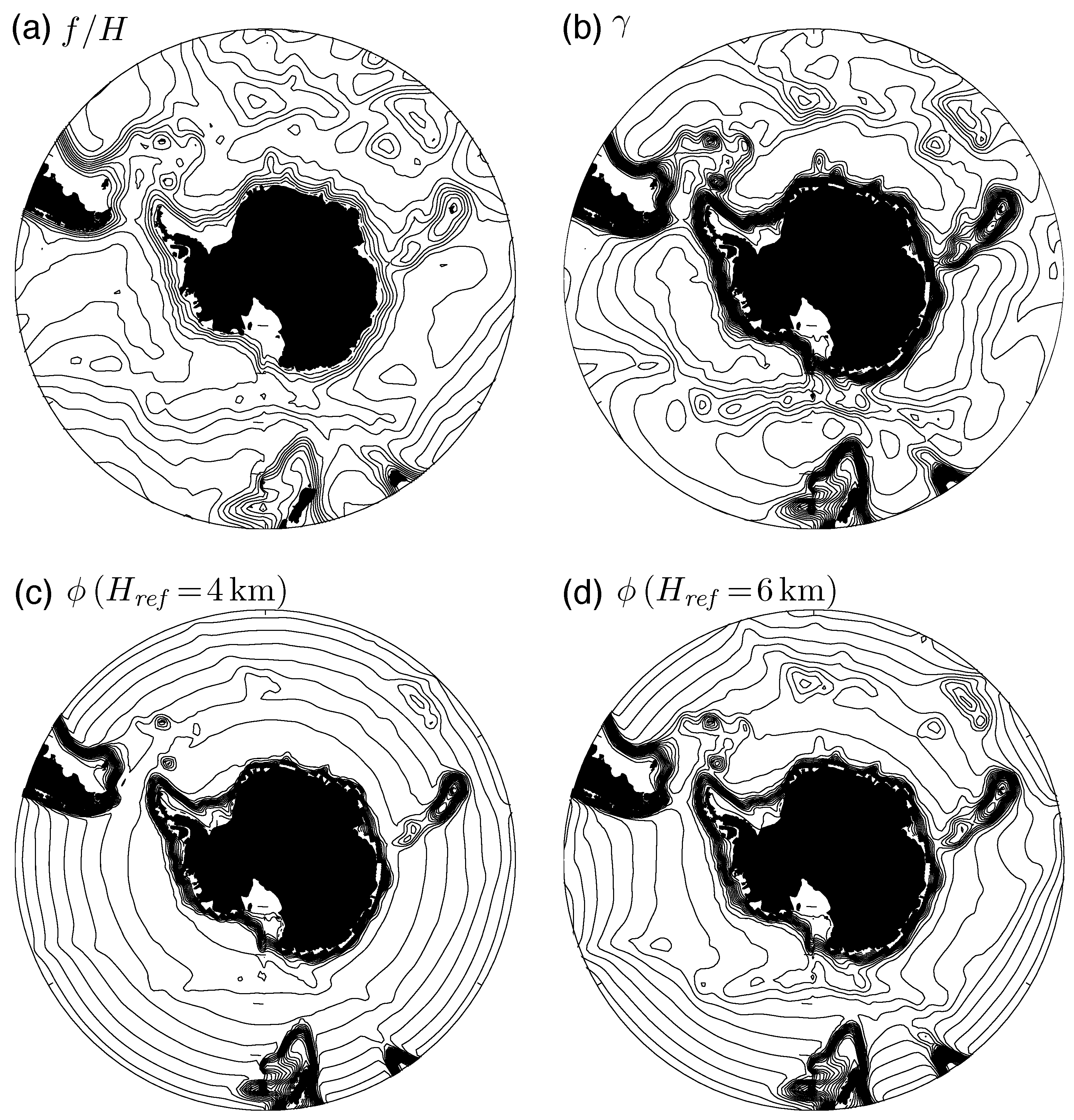
  • Long Rossby waves propagate along the same path as followed by the mean surface geostrophic flow, characteristics that are intermediate to f and f / H contours. For realistic Southern Ocean parameters, these characteristics are nearly zonal, with only slight deflections over major topographic features, aside from the Kerguelan Plateau which represents a more substantial obstacle.
  • The quasi-zonal propagation of long Rossby waves breaks down catastrophically in regions of closed f / H contours where, by analogy with the simpler two-layer model, the long Rossby waves can be expected to partially jump across the closed f / H contour.
  • In the absence of topographic variations, the Rossby propagation speed consists of an intrinsic Rossby speed, slightly modified from the classical Rossby speed to account for finite ocean depth, and Doppler shifting by the depth-mean flow, consistent with an earlier result obtained by Salmon [15]. This Doppler shift dominates for realistic Southern Ocean parameters, consistent with the observed eastward propagation of Southern Ocean anomalies in surface altimetric observations.
The model analysed in this paper relies on a number of overly restrictive assumptions. Firstly, the assumption of planetary geostrophic dynamics clearly breaks down in the presence of major topographic obstacles such as the Kerguelan Plateau, where inertial boundary layers, separated jets and short Rossby waves are each generated, e.g., [38,39,40]. Secondly, the ansatz of uniform potential vorticity on density surfaces is a convenient analytical and conceptual device in isolating the dynamical effects of the boundary conditions from the interior dynamics but is an extremely crude model of the hydrography observed in the Southern Ocean. More general functional relations between the mean potential vorticity, buoyancy and Montgomery potential will result in higher baroclinic Rossy wave modes, which are excluded in the present model. Thirdly, the model has excluded any explicit wind and buoyancy forcing, although such forcing is included in the more general theoretical approach of Salmon [15]. Fourthly, the effects of compressibility, and the separate contributions to the buoyancy from temperature and salinity, have been completely ignored. While common in practise in theoretical models of the ocean circulation (see [18,41]) for reviews, this simplification is purely for analytic convenience and not justified; the duality noted by [42] between the Boussinesq and non-Boussinesq hydrostatic equations of motion may provide a means of incorporating compressibility effects in a more consistent manner cf. [43,44].
Finally, it is important to emphasise that the theory presented in this paper applies only to long Rossby waves described by planetary geostrophic dynamics. In contrast, the propagating anomalies observed by satellite altimeter measurements of sea surface elevation are mostly nonlinear in the sense that the eddy velocities exceed the Rossby wave speed [2,3] such that planetary geostrophic dynamics are invalid. While these nonlinear anomalies do appear to propagate at roughly the long Rossby wave speed at mid latitudes [2,3], and in the Southern Ocean if the long Rossby wave speed is Doppler shifted by the depth-mean velocity [6], the present analysis does not predict the speed at which nonlinear anomalies should propagate, nor why. There are competing mechanisms for the zonal propagation speed of nonlinear eddies—for example, the existence of a critical layer in any baroclinically unstable current at which the local zonal velocity and intrinsic phase speed of the unstable mode match [45,46,47,48]. The existence of a critical layer means that the phase speed of the most unstable mode must lie within the envelope of zonal velocities of the mean current; in the case of the ACC, this means that the most unstable mode is eastward propagating, at a speed no greater than that of the surface zonal velocity (see also [28,29,49,50].

Acknowledgments

The author is grateful to Chris Hughes, Remi Tailleux, Andy Thompson and anonymous reviewers for useful suggestions that led to an improved manuscript. The author also thanks Rich Pawlowicz for making his M_Map mapping package available, used in the production of Figure 2, Figure 3 and Figure 4.

Conflicts of Interest

The author declares no conflict of interest.

Abbreviations

The following abbreviations are used in this manuscript:
MDPI
Multidisciplinary Digital Publishing Institute
ACC
Antarctic Circumpolar Current
JEBAR
Joint Effect of Baroclinicity and Relief

Appendix A. Derivation of Streamfunction of the Depth-Integrated Flow

Here, we outline the derivation of the expression Equation (33) for the depth-integrated streamfunction. First, we note that the depth-integrated velocity can be rewritten, using Equation (12), as
H 0 u ¯ d z = b ¯ b b ¯ s f u ¯ a b ¯ d b ¯ = b ¯ b b ¯ s k × b M ¯ a b ¯ d b ¯ ,
where b is the gradient operator evaluated along a buoyancy surface. Thus, defining the streamfunction for the depth-integrated flow, ψ, such that
H 0 u ¯ d z = k × ψ ¯ ,
we can identify:
ψ ¯ = b ¯ b b ¯ s M ¯ a b ¯ d b ¯ M ¯ s a b ¯ s b ¯ s + M ¯ b a b ¯ b b ¯ b .
Again using Equation (12) alongside Equations (26) and (28) gives:
ψ ¯ = H 0 M ¯ f d z ϕ a b ¯ s + H r e f b ¯ b a .
Now, substituting for M ¯ using the time-mean of Equation (9), substituting for p ¯ using Equation (32), substituting for b ¯ and b ¯ b using Equations (13) and (14), and evaluating the integrals, the final result follows:
ψ ¯ = b ¯ s a 2 ϕ H r e f e a H / f a H f ( H H r e f ) e a H / f ϕ ( b ¯ s ) a d b ¯ s ,
which is Equation (33).

References

  1. Munk, W.H.; Palmén, E. Note on the dynamics of the Antarctic Circumpolar Current. Tellus 1951, 3, 53–55. [Google Scholar] [CrossRef]
  2. Chelton, D.B.; Schlax, M.G.; Samelson, R.M.; de Szoeke, R.A. Global observations of large oceanic eddies. Geophys. Res. Lett. 2007, 34. [Google Scholar] [CrossRef]
  3. Chelton, D.B.; Schlax, M.G.; Samelson, R.M. Global observations of nonlinear mesoscale eddies. Prog. Oceanogr. 2011, 91, 167–216. [Google Scholar] [CrossRef]
  4. Hughes, C.W.; Jones, M.S.; Carnochan, S. Use of transient features to identify eastward currents in the Southern Ocean. J. Geophys. Res. 1998, 103, 2929–2942. [Google Scholar] [CrossRef]
  5. Hughes, C.W. Nonlinear vorticity balance of the Antarctic Circumpolar Current. J. Geophys. Res. 2005, 110. [Google Scholar] [CrossRef]
  6. Klocker, A.; Marshall, D.P. Advection of baroclinic eddies by depth mean flow. Geophys. Res. Lett. 2014, 41, 3517–3521. [Google Scholar] [CrossRef]
  7. Sarkisyan, A.S. Principles of Theory and Computation of Ocean Currents; Gidrometeoizdat: Leningrad, Russia, 1966. [Google Scholar]
  8. Sarkisyan, A.S.; Ivanov, V.F. Joint effect of baroclinicity and bottom relief as an important factor in the dynamics of sea currents. Izv. Akad. Nauk. SSSR Fiz. Atmos. Okeana 1971, 7, 173–188. [Google Scholar]
  9. Cane, M.A.; Kamenkovitch, V.M.; Krupiysky, A. On the utility and disutility of JEBAR. J. Phys. Oceanogr. 1998, 28, 519–526. [Google Scholar] [CrossRef]
  10. Marshall, D. Influence of topography on the large-scale ocean circulation. J. Phys. Oceanogr. 1995, 25, 1622–1635. [Google Scholar] [CrossRef]
  11. Marshall, D. Topographic steering of the Antarctic Circumpolar Current. J. Phys. Oceanogr. 1995, 25, 1636–1650. [Google Scholar] [CrossRef]
  12. Marshall, D.P.; Stephens, J.C. On the insensitivity of the wind-driven circulation to bottom topography. J. Mar. Res. 2001, 59, 1–27. [Google Scholar] [CrossRef]
  13. Killworth, P.D.; Hughes, C.W. The Antarctic Circumpolar Current as a free equivalent-barotropic jet. J. Mar. Res. 2002, 60, 19–45. [Google Scholar] [CrossRef]
  14. de Szoeke, R.A. Wind-driven mid-ocean baroclinic gyres over topography: A circulation equation extending the Sverdrup relation. J. Mar. Res. 1985, 43, 793–824. [Google Scholar] [CrossRef]
  15. Salmon, R. Generalized two-layer models of ocean circulation. J. Mar. Res. 1994, 52, 865–908. [Google Scholar] [CrossRef]
  16. Marshall, D.P. Rossby wormholes. J. Mar. Res. 2011, 69, 309–330. [Google Scholar] [CrossRef]
  17. Welander, P. An advective model of the ocean thermocline. Tellus 1959, 11, 309–318. [Google Scholar] [CrossRef]
  18. Pedlosky, J. Geophysical Fluid Dynamics; Springer-Verlag: New York, NY, USA, 1987. [Google Scholar]
  19. De Verdiere, A. On mean flow instabilities within the planetary geostrophic equations. J. Phys. Oceanogr. 1986, 16, 1981–1984. [Google Scholar] [CrossRef]
  20. Welander, P. Some exact solutions to the equations describing an ideal-fluid thermocline. J. Mar. Res. 1971, 29, 60–68. [Google Scholar]
  21. Marshall, J.; Olbers, D.; Ross, H.; Wolff-Gladrow, D. Potential vorticity constraints on the dynamics and hydrography of the Southern Ocean. J. Phys. Oceanogr. 1993, 23, 465–487. [Google Scholar] [CrossRef]
  22. Kartsen, R.H.; Marshall, J. Testing theories of the vertical stratification of the ACC against observations. Dyn. Atmos. Oceans 2002, 36, 233–246. [Google Scholar]
  23. Stommel, H. A survey of ocean current theory. Deep Sea Res. 1957, 4, 149–184. [Google Scholar] [CrossRef]
  24. Marshall, D.P.; Munday, D.R.; Allison, L.C.; Hay, R.J.; Johnson, H.L. Gill’s model of the Antarctic Circumpolar Current, revisited: The role of latitudinal variations in wind stress. Ocean Modell. 2016, 97, 37–51. [Google Scholar] [CrossRef]
  25. Killworth, P.D. An equivalent barotropic mode in the Fine Resolution Antarctic Model. J. Phys. Oceanogr. 1992, 22, 1379–1386. [Google Scholar] [CrossRef]
  26. Tailleux, R.; McWilliams, J.C. Acceleration, creation, and depletion of wind-driven, baroclinic Rossby waves over an ocean ridge. J. Phys. Oceanogr. 2000, 30, 2186–2213. [Google Scholar] [CrossRef]
  27. Tailleux, R.; McWilliams, J.C. Energy propagation of long extratropical Rossby waves over slowly varying zonal topography. J. Fluid Mech. 2002, 473, 295–319. [Google Scholar] [CrossRef]
  28. Smith, K.S.; Marshall, J. Evidence for enhanced eddy mixing at mid-depth in the Southern Ocean. J. Phys. Oceanogr. 2009, 39, 50–69. [Google Scholar] [CrossRef]
  29. Abernathey, R.; Marshall, J.; Mazloff, M.; Shuckburgh, E. Enhancement of Mesoscale Eddy Stirring at Steering Levels in the Southern Ocean. J. Phys. Oceanogr. 2010, 40, 170–184. [Google Scholar] [CrossRef] [Green Version]
  30. Meredith, M.P.; Woodworth, P.L.; Chereskin, T.K.; Marshall, D.P.; Allison, L.C.; Bigg, G.R.; Donahue, K.; Heywood, K.J.; Hughes, C.W.; Hibbert, A.; et al. Sustained monitoring of the Southern Ocean at Drake Passage: Past achievements and future priorities. Rev. Geophys. 2011, 49. [Google Scholar] [CrossRef]
  31. Held, I.M. Stationary and quasi-stationary eddies in the extratropical troposphere: Theory. In Large-Scale Dynamical Processes in the Atmosphere; Hoskins, B.J., Pearce, R.P., Eds.; Academic Press: Cambridge, MA, USA, 1983; pp. 127–168. [Google Scholar]
  32. Liu, Z.Y. Planetary waves in the thermocline: Non-Doppler-shift mode, advective mode and Green mode. Q. J. R. Met. Soc. 1999, 125, 1315–1339. [Google Scholar] [CrossRef]
  33. Colin de Verdiere, A.; Tailleux, R. The interaction of a baroclinic mean flow with long Rossby waves. J. Phys. Oceanogr. 2005, 35, 865–879. [Google Scholar] [CrossRef]
  34. Samelson, R. An effective-β vector for linear planetary waves on a weak mean flow. Ocean Modell. 2010, 32, 170–174. [Google Scholar] [CrossRef]
  35. Killworth, P.D.; Chelton, D.B.; de Szoeke, R.A. The speed of observed and theoretical long extratropical planetary waves. J. Phys. Oceanogr. 1997, 27, 1946–1966. [Google Scholar] [CrossRef]
  36. Dewar, W.K. On ‘too fast’ baroclinic planetary waves in the general circulation. J. Phys. Oceanogr. 1998, 28, 1739–1758. [Google Scholar] [CrossRef]
  37. De Szoeke, R.A.; Chelton, D.B. The modification of long planetary waves by homogeneous potential vorticity layers. J. Phys. Oceanogr. 1999, 29, 500–511. [Google Scholar] [CrossRef]
  38. Tansley, C.E.; Marshall, D.P. Flow past a cylinder on a β-plane, with application to Gulf Stream separation and the Antarctic Circumpolar Current. J. Phys. Oceanogr. 2001, 31, 3274–3283. [Google Scholar] [CrossRef]
  39. Tansley, C.E.; Marshall, D.P. On the dynamics of wind-driven circumpolar currents. J. Phys. Oceanogr. 2001, 31, 3258–3272. [Google Scholar] [CrossRef]
  40. Hallberg, R.W.; Gnanadesikan, A. The role of eddies in determining the structure and response of the wind-driven Southern Hemisphere overturning: Results from the modeling eddies in the Southern Ocean (MESO) project. J. Phys. Oceanogr. 2006, 36, 2232–2252. [Google Scholar] [CrossRef]
  41. Salmon, R. Lectures on Geophysical Fluid Dynamics; Oxford University Press: Oxford, UK, 1998. [Google Scholar]
  42. De Szoeke, R.A.; Samelson, R.M. The duality between the Boussinesq and non-Boussinesq hydrostatic equations of motion. J. Phys. Oceanogr. 2002, 32, 2194–2203. [Google Scholar] [CrossRef]
  43. Losch, M.; Adcroft, A.; Campin, J.M. How Sensitive Are Coarse General Circulation Models to Fundamental Approximations in the Equations of Motion? J. Phys. Oceanogr. 2004, 34, 306–319. [Google Scholar] [CrossRef]
  44. Marshall, J.; Adcroft, A.; Campin, J.M.; Hill, C. Atmosphere-Ocean Modeling Exploiting Fluid Isomorphisms. Mon. Weather Rev. 2004, 132, 2882–2894. [Google Scholar] [CrossRef]
  45. Charney, J.G. On the scale of atmospheric motions. Geofys. Publ. 1948, 17, 1–17. [Google Scholar]
  46. Eady, E.T. Long waves and cyclone waves. Tellus 1949, 1, 33–52. [Google Scholar] [CrossRef]
  47. Green, J.S.A. A problem in baroclinic instability. Quart. J. R. Meteor. Soc. 1960, 86, 237–251. [Google Scholar] [CrossRef]
  48. Bretheron, F.P. Critical layer instability in baroclinic flows. Quart. J. R. Meteor. Soc. 1966, 92, 325–334. [Google Scholar] [CrossRef]
  49. Treguier, A.M. Evaluating eddy mixnig coefficients from eddy-resolving ocean models: A case study. J. Mar. Res. 1999, 57, 89–108. [Google Scholar] [CrossRef]
  50. Cerovecki, I.; Plumb, R.A.; Heres, W. Eddy transport and mixing in a wind- and buoyancy-driven jet on the sphere. J. Phys. Oceanogr. 2009, 39, 1133–1149. [Google Scholar] [CrossRef]
Figure 1. Schematic diagram illustrating the key ingredients of the model. In the ocean interior, the ansatz that the potential vorticity is a linear function of buoyancy imposes a known exponential decay of buoyancy (thick solid contours) with depth. The solution is therefore determined by conservation of buoyancy along the sea surface, b s ( x , y ) , and along the sea floor, b b (see Section 3). The total ocean depth is H ( x , y ) and the path of the surface streamlines in equilibrium is given by the characteristic function, ϕ ( x , y ) (thin solid contours, see Section 4).
Fluids 01 00017 g001
Figure 2. Contours of: (a) f / H ; (b) γ; (c) ϕ with H ref = 4 km ; (d) ϕ with H ref = 6 km . The contours of ϕ represent the characteristics along which the surface geostrophic flow is directed in the absence of forcing (Section 4) and also along which long Rossby waves propagate (Section 5).
Fluids 01 00017 g002
Figure 3. Illustrative steady-state solution with H r e f = 4 km . The figure shows buoyancy at the sea surface, b s ¯ , which is a prescribed function of the characteristic function, ϕ , and also a vertical section of the buoyancy, b, at the longitude 150W. The buoyancy is related to (neutral) density anomalies, δ ρ , by b = g δ ρ / ρ 0 , where g is the gravitational acceleration, and so the values should be multiplied by a factor of roughly 10 2 to convert to (neutral) density anomalies in kg · m 3 .
Fluids 01 00017 g003
Figure 4. Flow fields in the steady-state solution with H r e f = 4 km . (a) depth-integrated streamfunction, ψ ¯ (Sv); (b) geostrophic streamlines, p ¯ / ρ 0 , at 0 km ( m 2 · s 2 ); (c) geostrophic streamlines, p ¯ / ρ 0 , at 2 km ( m 2 · s 2 ); (d) geostrophic streamlines, p ¯ / ρ 0 , at 4 km ( m 2 · s 2 ).
Fluids 01 00017 g004
Figure 5. Graph of coth ( H / 2 H strat ) 2 H strat / H versus H / 2 H strat .
Fluids 01 00017 g005

