Sensitivity of Codispersion to Noise and Error in Ecological and Environmental Data


1
Departamento de Matemática, Universidad Técnica Federico Santa María, Avenida España 1680, Valparaíso 2340000, Chile
2
School of Science, Auckland University of Technology, 55 Wellesley Street East, Auckland 1010, New Zealand
3
Instituto de Estadística, Pontificia Universidad Católica de Valparaíso, Av. Brasil 2950, Valparaíso 2340000, Chile
4
Harvard Forest, Harvard University, 324 North Main Street, Petersham, MA 01366, USA
*
Author to whom correspondence should be addressed.
Forests 2018, 9(11), 679; https://doi.org/10.3390/f9110679
Submission received: 26 September 2018
/
Revised: 19 October 2018
/
Accepted: 21 October 2018
/
Published: 29 October 2018
(This article belongs to the Special Issue 3D Remote Sensing Applications in Forest Ecology: Composition, Structure and Function)
Abstract
:Understanding relationships among tree species, or between tree diversity, distribution, and underlying environmental gradients, is a central concern for forest ecologists, managers, and management agencies. The spatial processes underlying observed spatial patterns of trees or edaphic variables often are complex and violate two fundamental assumptions—isotropy and stationarity—of spatial statistics. Codispersion analysis is a new statistical method developed to assess spatial covariation between two spatial processes that may not be isotropic or stationary. Its application to data from large forest plots has provided new insights into mechanisms underlying observed patterns of species distributions and the relationship between individual species and underlying edaphic and topographic gradients. However, these data are not collected without error, and the performance of the codispersion coefficient when there is noise or measurement error (“contamination”) in the data heretofore has been addressed only theoretically. Here, we use Monte Carlo simulations and real datasets to investigate the sensitivity of codispersion to four types of contamination commonly seen in many forest datasets. Three of these involved comparing codispersion of a spatial dataset with a contaminated version of itself. The fourth examined differences in codispersion between tree species and soil variables, where the estimates of soil characteristics were based on complete or thinned datasets. In all cases, we found that estimates of codispersion were robust when contamination was relatively low (<15%), but were sensitive to larger percentages of contamination. We also present a useful method for imputing missing spatial data and discuss several aspects of the codispersion coefficient when applied to noisy data to gain more insight about the performance of codispersion in practice.
1. Introduction
Spatial associations are a fundamental aspect of most ecological and environmental data, including size-frequency distributions of trees, their co-occurrence and diversity, and the relationships between trees and underlying edaphic characteristics or topographic variables such as distance to water table, slope, and aspect. Although accounting for spatial covariation has become routine in ecological data analysis [1], forest ecologists have been slower to appreciate and account for anisotropic patterns and processes (but see, e.g., [2]). Codispersion [3] measures lag-dependent spatial covariation in two or more spatial processes, which may be anisotropic. Codispersion recently has been used to examine interactions between species, and relationships between species distributions and underlying environmental gradients in large (>25-ha) forest dynamics plots. These analyses have provided new insights into potential ecological processes that underlie observed patterns in co-occurrence between pairs of tree species [4], in relationships between attributes of individual tree species and underlying edaphic characteristics [5], and in forest structure through time [6].
All applications of codispersion analysis that have been published to date have assumed either that there are no errors in the datasets or that any errors that are present would have no effect on the analysis. These assumptions are clearly unrealistic. The goal of this paper is to better understand how sensitive the codispersion coefficient is to different types of noise and measurement error (“contamination”) in analyzed datasets, and address the implication of this sensitivity for spatial analysis of data collected on forest structure and composition. We approach this goal by using Monte Carlo simulation studies to examine several classes of noise that we would expect to occur in datasets or images analyzed using codispersion. Our focus here is on the analysis of data gathered from large forest plots either by remote sensing or on-the-ground sampling that are used to describe forest structure or test hypotheses regarding the relationship between spatial distribution of trees and edaphic variables. However, the results are generalizable to any dataset for which there is either measurement error in the spatial data collected or process error in the spatial models that are used in subsequent analysis.
Measurement (observation) error can occur in several ways. For example, trees can be misidentified by observers or pixels in remotely-sensed images can be misclassified. Either can affect inferences about interspecific relationships or associations between plant species and edaphic characteristics. To examine the effect of these “simple” observation errors (misidentification or misspecification) on codispersion analysis, we added statistical noise to a fixed number of random points (or pixels) in a dataset (here, a remotely-sensed image of a forest stand) either as white noise (spatially independent and identically distributed) or as a spatially-dependent process.
Another type of measurement error would be when clusters of individuals are missed or overlooked in a census of a forest stand, either through human error of if clusters of pixels in a remotely-sensed image are unmeasurable because of cloud cover. Spatial analysis of such data would require that these gaps be filled, and we present and assess the consequences of different algorithms for interpolation prior to calculation of codispersion [7].
The flip-side of interpolating missing data is to smooth sparsely-collected data (e.g., soils data smoothed using kriging, splines, etc.); the smoothed surface is subsequently sampled at specific (otherwise unsampled) points to test for associations between individual tree species and (estimated) local environmental (e.g., soil) properties. Errors here can occur because of mis-specified models or because too few data are available to construct a reliable smoothed surface. We examined these issues for the assessment of relationships between trees and soil characteristics when different amounts of modeled error were introduced into the environmental data as a result of kriging surfaces derived from complete or “thinned” datasets; the latter mimicked datasets with missing values.
In all of these cases, the effects of error were tested in one of two ways. For single datasets (images) to which we added random or clustered errors, we calculated the codispersion between the original dataset (image) and the contaminated version of itself. In those cases, we examined differences between high- and lower-quality (error-filled) images. For species–soil relationships, we compared the results obtained using kriged surfaces derived from the complete sample of soil properties versus those derived from soil samples missing random points (the “thinned”) data.
In Section 2, we describe the codispersion coefficient and a way to visualize it (i.e., a codispersion map). We also specify the different types of contamination and observation error that we added to both real and simulated datasets, and describe the method we used for imputing missing data. Results are presented in Section 3, and discussed in Section 4. Technical details on simulation and imputation algorithms are given in Appendix A.
2. Methods
2.1. Preliminaries and Notation
Here, we briefly introduce the notion of the codispersion coefficient, first described in [8], and the graphical codispersion “map” developed in [3] and applied to forest data in [4]. These statistical entities characterize the spatial correlation between two spatial processes as a function of the separation distance (lag) between the points.
Let us consider two spatial processes and , where both processes are defined on a part of a region (or on a rectangular lattice ). For two intrinsically stationary processes and , the codispersion coefficient is defined as
for This coefficient shares several properties with Pearson’s correlation coefficient (r). First, the structure of is computationally similar to r. Second, like r, which facilitates its interpretation because the upper and lower bounds define perfect negative or positive spatial association, respectively. Unlike r, however, depends on the spatial lag , which emphasizes that spatial correlation is a value associated with a distance on the plane. This facilitates the computation of correlation for different distances and directions on the space. In this sense, Pearson’s correlation is a crude measure of the spatial association between two processes.
For n sampling sites the sample-based estimator of (1), based on the method of moments, is
where , is a tolerance region around , and denotes the Euclidean norm in . The estimator of the codispersion coefficient given in Equation (2) can be computed for any fixed spatial lag . This computation can be difficult if the number of points is small or if is an empty set. We emphasize that the empirical estimator of the codispersion coefficient makes real sense when the processes are defined on a finite rectangular grid in a two-dimensional space that corresponds to the assessment of the similarities between two digital images [9].
When the codispersion coefficient is computed for many directions, it is useful to display those values on a single graph. Vallejos [3] suggested a graphical tool called the codispersion map to visualize the spatial correlation between two sequences on a plane. The estimated values illustrated by the codispersion map are based on Equation (2). A finite grid on the plane is first defined on which the codispersion coefficient will be computed for each location in that grid. The codispersion map itself is the graph of versus ; plotting the codispersion map summarizes the information about the spatial association between two sequences in a radial way on the plane circumscribing the map in a semicircle of fixed radius.
Note that does not capture similarity that is related to the patterns or shapes that are present in the images. Rather, it captures the spatial dependence between the processes for a given lag distance .
2.2. Types of Error
In spatial modeling and time series, several types of error (a.k.a. noise) can be specified [10,11]. Here, we considered five types of error frequently observed in spatial data; our examples are drawn from data collected from forest stands, which to date have been the primary testbed for ecological applications of codispersion analysis.
- 1.
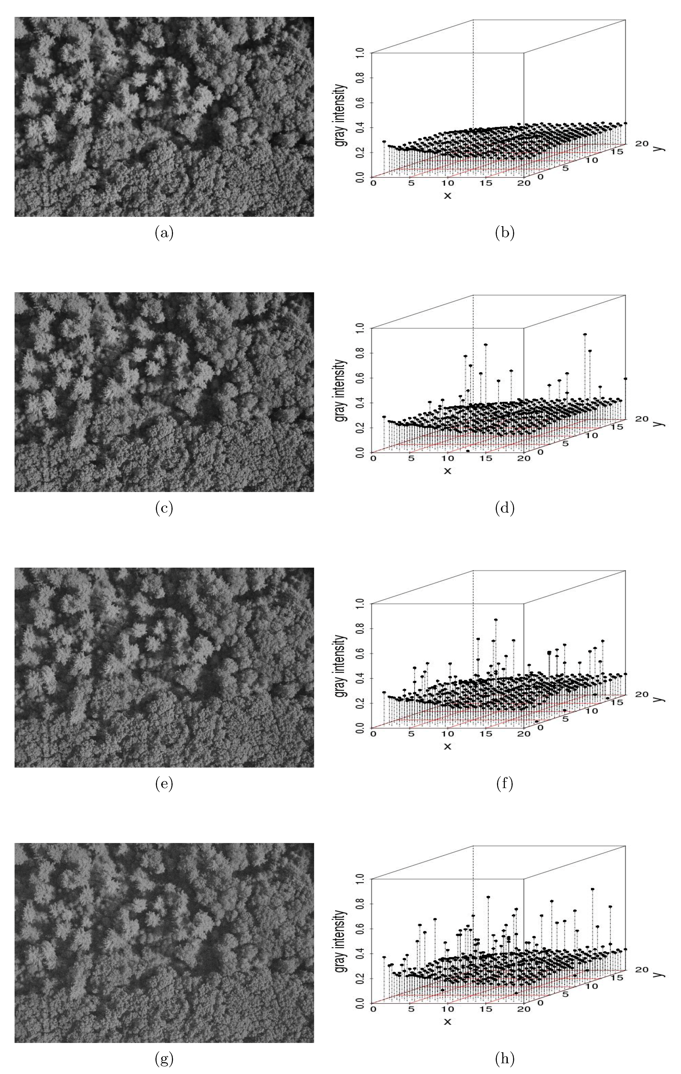
- “Salt-and-pepper” noise on an image: Salt-and-pepper noise—so-called because of its resemblance to dust on images that appears to have been distributed by a salt or pepper shaker—is used widely in image processing and computational statistics to represent real distortions [12] and to generate different scenarios via Monte Carlo simulation [13]. Salt-and-pepper noise can be added to an image using a simple algorithm:Assume that is the original image whose individual observations are points or pixels representing leaves or trees and is the contaminated image with salt-and-pepper noise such that the additive noise is drawn from a normal distribution with mean = 0 and variance , with , where is the variance of . The contamination is located randomly in space such that a small percentage of observations are corrupted with a probability [3]. Specifically,where the is an outlier generating process such that is a zero-one process with and , and .We used Monte Carlo simulations of (3) to generate salt-and-pepper noise on a 5616 × 3744-pixel aerial image of a forest stand at Harvard Forest in Petersham, MA, USA (Figure 1). We considered , and the percentage of contamination We conjectured that the codispersion coefficient would be robust for That is, for relatively small amounts of measurement error, we could still recover the relevant spatial information present in the remotely-sensed image.In Figure 1a, we illustrate the noise-free image. Figure 1c,e,g is contaminated versions of the original one when . The corresponding perspective plots shown in Figure 1b,d,f,h depict the effect of contamination on the gray intensities. The greater the contamination, the greater the dispersion, which is plotted on the z-axis of the three-dimensional scatter plots displayed in Figure 1.We then compared the codispersion calculated for the original image to that calculated for the contaminated images. In addition to the reference image shown in Figure 1a, we considered other aerial images. The codispersion maps of these images are presented in the supplementary material for this paper. We emphasize that the computation of the codispersion coefficient requires that both processes are measured over the same domain, thus the codispersion between a reference image and its contaminated versions make sense. To address the codispersion between two images taken from different scenarios (for instance, images displayed in the supplementary material), rasterized versions of the original images could be considered following the guidelines given in [4].
- 2.
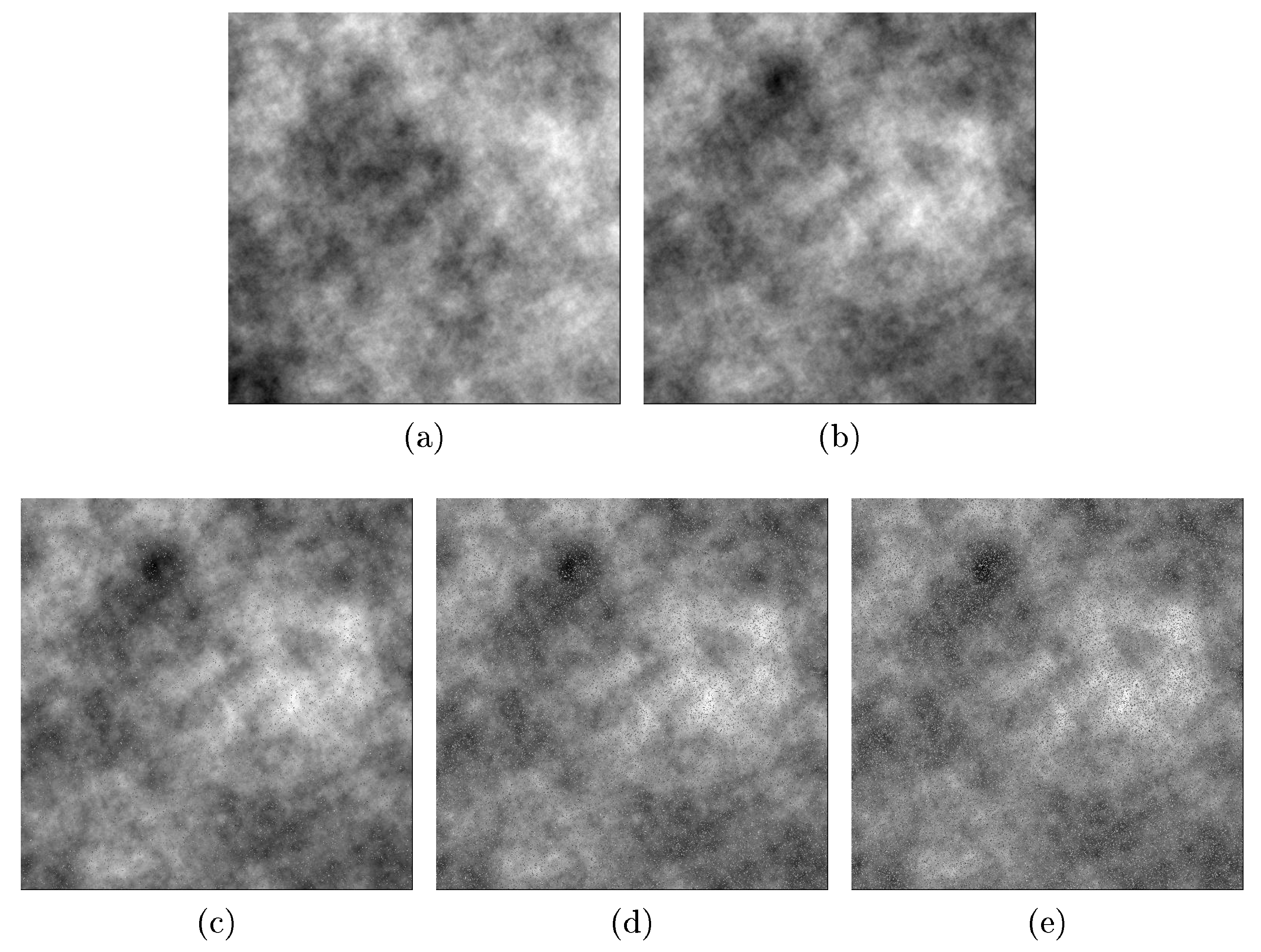
- Salt-and-pepper noise on dependent processes: More generally, Reference [14] extended the well known Matérn class of covariance functions to a multivariate random field. For multivariate Gaussian and second-order processes, the multivariate Matérn covariance function is defined aswhere is the distance lag, is a modified Bessel function of the second kind, is a spatial scale parameter, and is a smoothness parameters that defines the Hausdorff dimension and the differentiability of the sample paths. In particular, a Gaussian and second-order stationary process , has a bivariate Matérn covariance matrix ifwhere are the marginal covariance functions, with variance parameter , smoothness parameter , and scale parameter for . is the cross-covariance function, with correlation coefficient , smoothness parameter , and scale parameter . In all cases, is the function defined in Equation (4). The parsimonious bivariate Matérn model has the restrictionThe correlation between the spatial variables and is controlled by the parameter which allows one to generate bivariate Gaussian spatial processes with different levels of dependence. The spatial correlation defined by Equation (6) is not necessarily bounded by 1. Without loss of generality, it can be assumed that the mean of the bivariate process is zero, but the theory works well for any bivariate process with mean Any type of contamination can be applied over the generated dependence data. In this case, we applied salt-and-pepper noise.We generated dependent random fields from the bivariate Matérn class of covariance functions described in Equation (5) by Monte Carlo simulation using the R package RandomFields [15]. We then added the salt-and-pepper noise, varying the additional parameter , which represents the known correlation between processes and .Figure 2 shows one realization of size from a bivariate Gaussian process (images (a) and (b)) with correlation equal to 0.8, and , , and . Figure 2c,d,e show versions of (b) contaminated with salt-and-pepper noise with the percentage of contamination equal to 5%, 15%, and 25%, respectively. Because the Gaussian process is stationary, images (a) and (b) look very regular (approximately constant mean and variance), and any correlation between them (if it exists) is difficult to observe in the printed images. Other parameters used in the simulation study are , , , , and . The results are similar to the shown here, but with a codispersion map close to zero.
- 3.
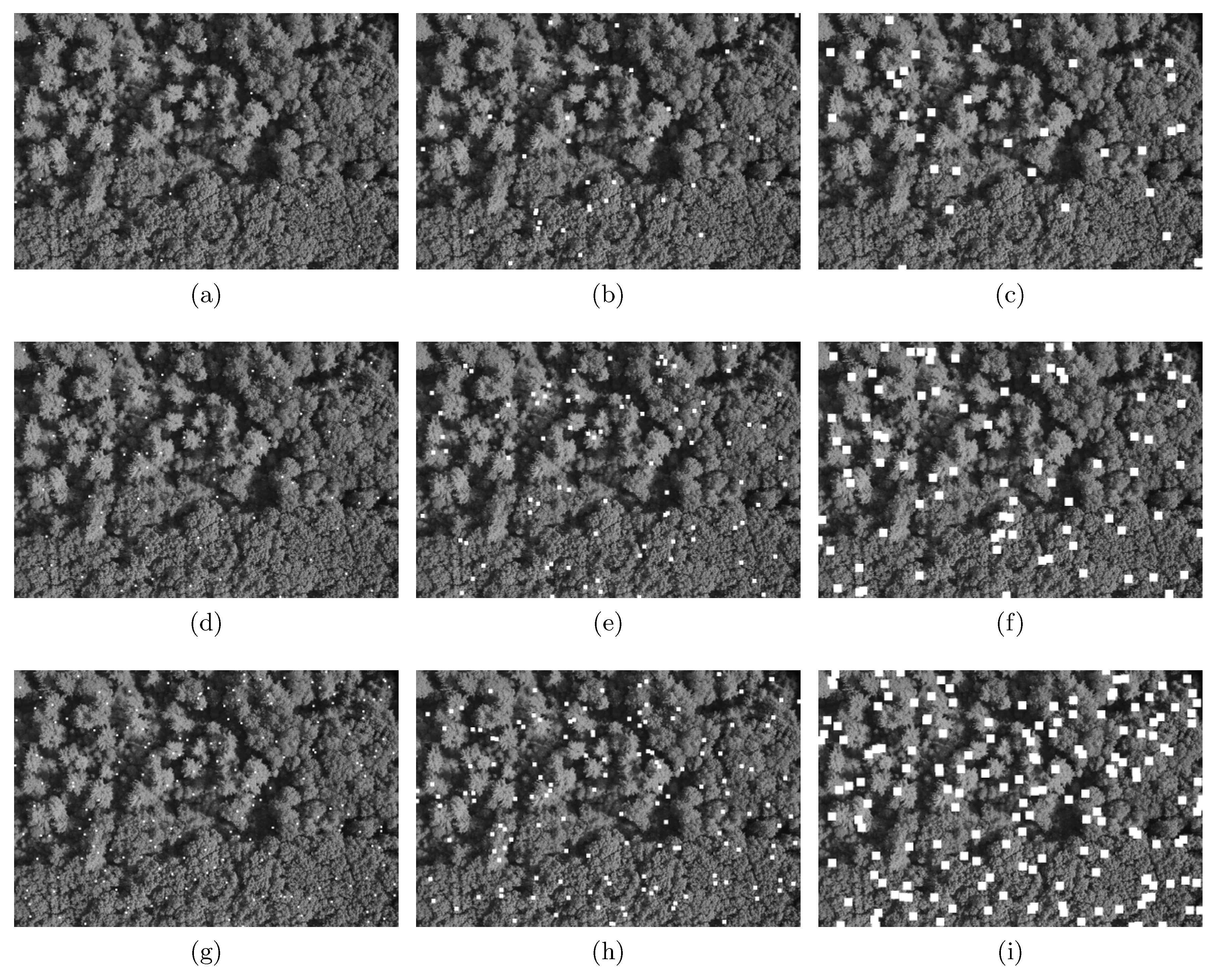
- Missing observations at random locations: We used the salt-and-pepper scheme to randomly delete n observations. We first defined the percentage of contamination (), and then deleted that many observations from the dataset. In practice, we replaced observations with non-observed (NA) at the randomly-selected locations. The main feature of these missing observations is that they are spatially independent of one another, but, for the posterior data analysis, they will remain fixed. The imputation algorithm described in the Appendix A was not applied here because codispersion calculations are not affected when the percentage of contamination is small.In Figure 3, we illustrate the missing-observations-at-random-locations with nine contaminated versions of the original image shown in Figure 1a. The columns show the effect of increasing the percentage of contamination (5%, 15%, and 25%, respectively), and the rows depict the effect of increasing the block size of contaminated pixels, which are , , and respectively. The contaminated pixels have been colored in white. NAs were ignored in the computation of the codispersion coefficients because for large gaps of missing observations the computation of the codispersion coefficient will be affected for those directions such that is less than the maximum diameter of the missing block.
- 4.
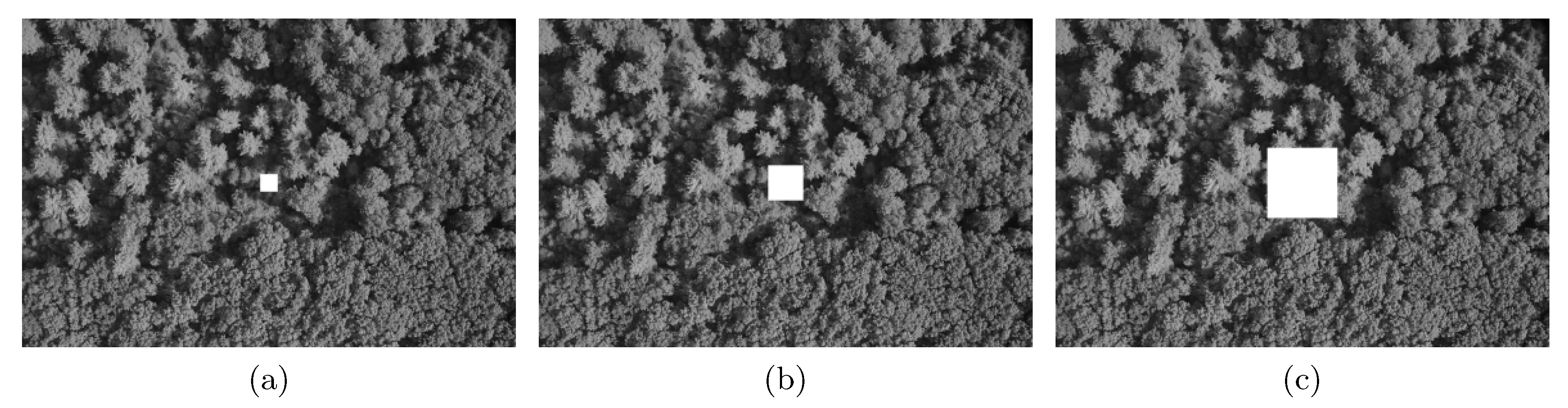
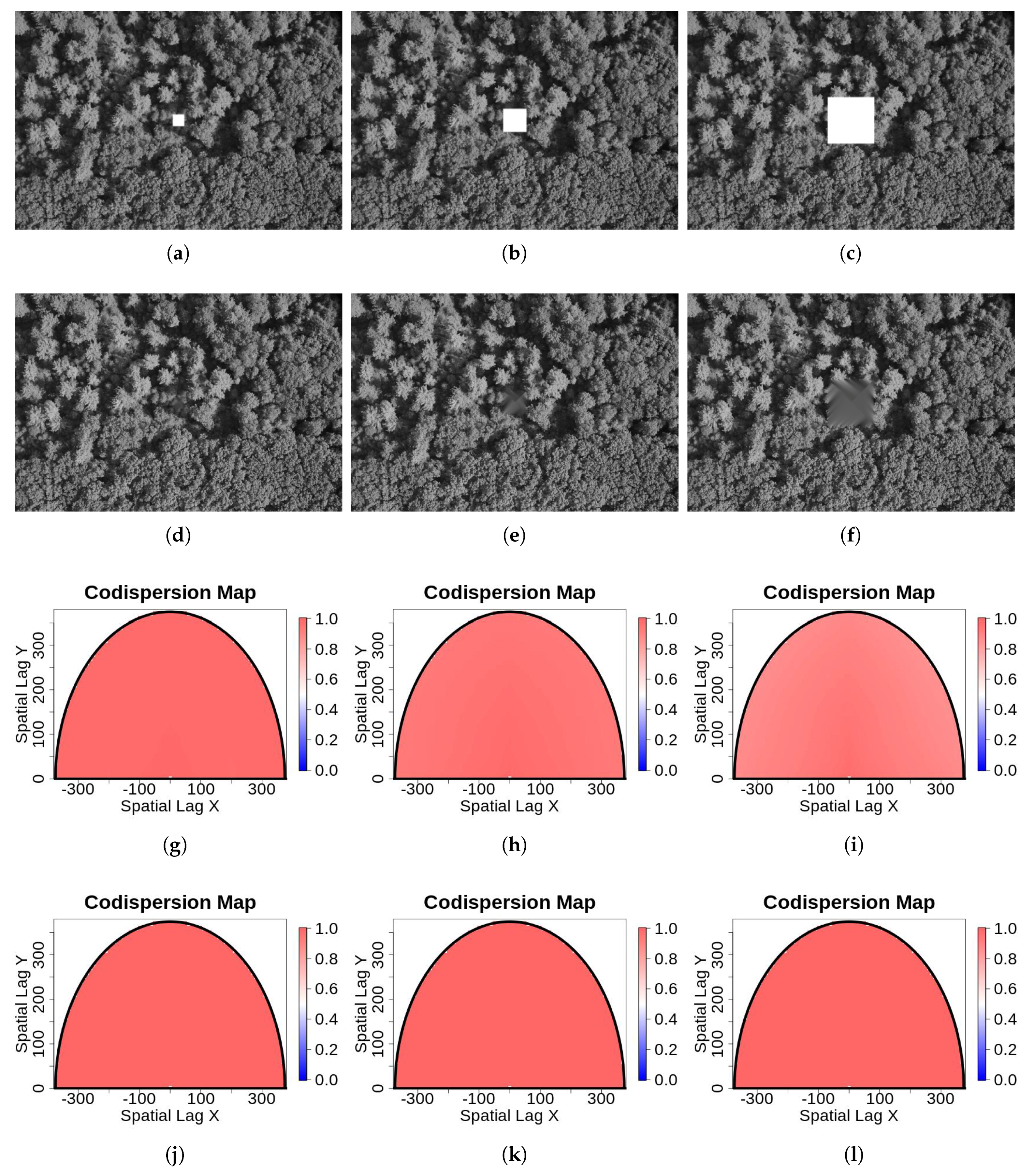
- Gaps resulting from clusters of missing observations: Missing values may be clustered, for example, either because of local difficulties in sampling or because large sections of a remotely-sensed image are obscured by, for example, clouds or shadows. We simulated clustered missing observations for the image shown in Figure 1a, given three different pixel sizes for the contaminated block: , , and (Figure 4). We used simple clustered geometries (squares) for ease of computation. The difference between the previous type of contamination and this one is that, in the former, the contamination consisted of several blocks of small size. Here, we introduced just one gap containing a large number of pixels, which, in Figure 4, is located for illustrative purposes in the center of the image. In our simulations and analysis, the size of the missing block and its location were fixed.To compute codispersion coefficients for datasets with such large blocks of missing data, we needed to fill the missing gaps (impute missing data) prior to computing the codispersion coefficient. We used and compared two different methods of imputation (gap-filling).First, the image with a missing gap was represented by a first-order spatial autoregressive process. The fitting of the parameters of the models was done via least-squares estimation following the guidelines given in [16]. This estimation method was studied in [17] and found to yield an approximated image of the original one X (see Algorithm 1 in the Appendix A).Second, to predict the values of the process in the locations belonging to the missing block, we applied Algorithm 1 to predict missing values in the four closest blocks to the missing gap as is illustrated in Figure A1. This prediction scheme is summarized in Algorithm 2 (Appendix A). Briefly, the first step represents the image intensity by an autoregressive process that assumes that the intensity of any pixel is a weighted average of the intensity of the surrounding pixels. This is a model-based alternative to the average or median commonly computed using the intensities of a moving window across the image. The second step predicts the missing values using similar autoregressive models to represent the surrounding blocks. The predicted value of a pixel belonging to the missing block is a weighted average where the weights are proportional to the distance from the missing pixel to the surrounding blocks.
- 5.
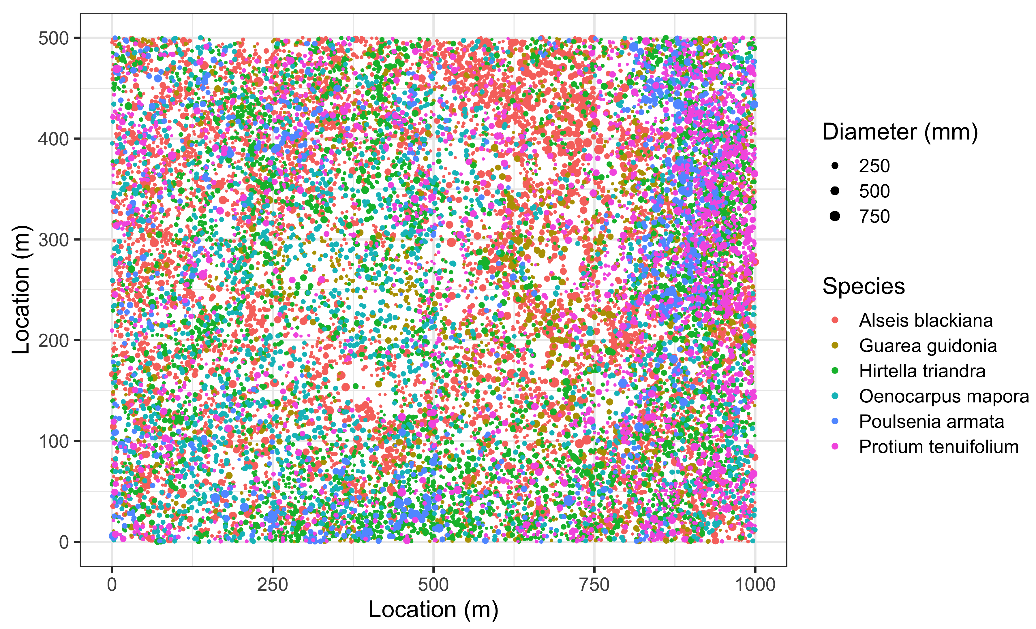
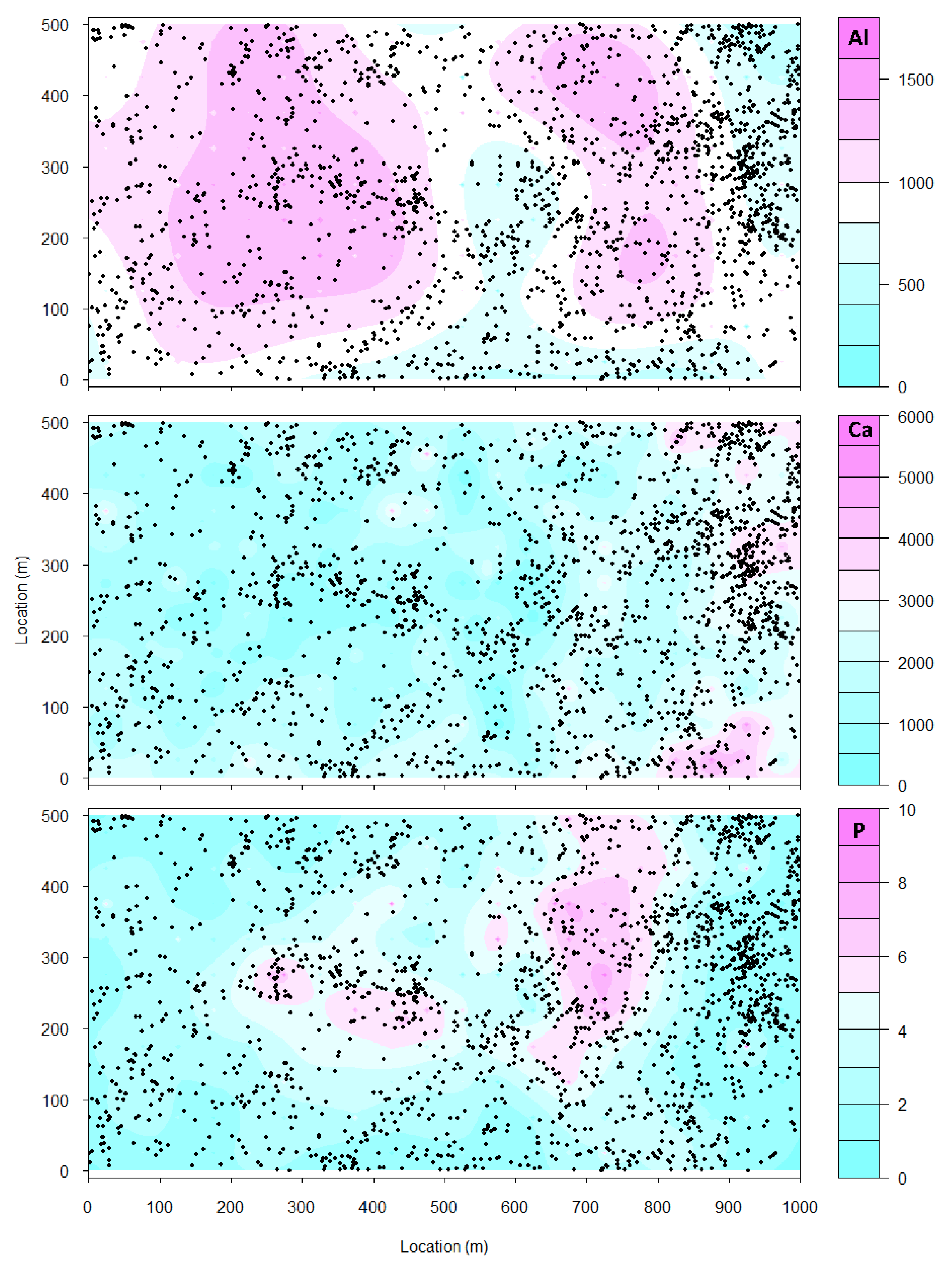
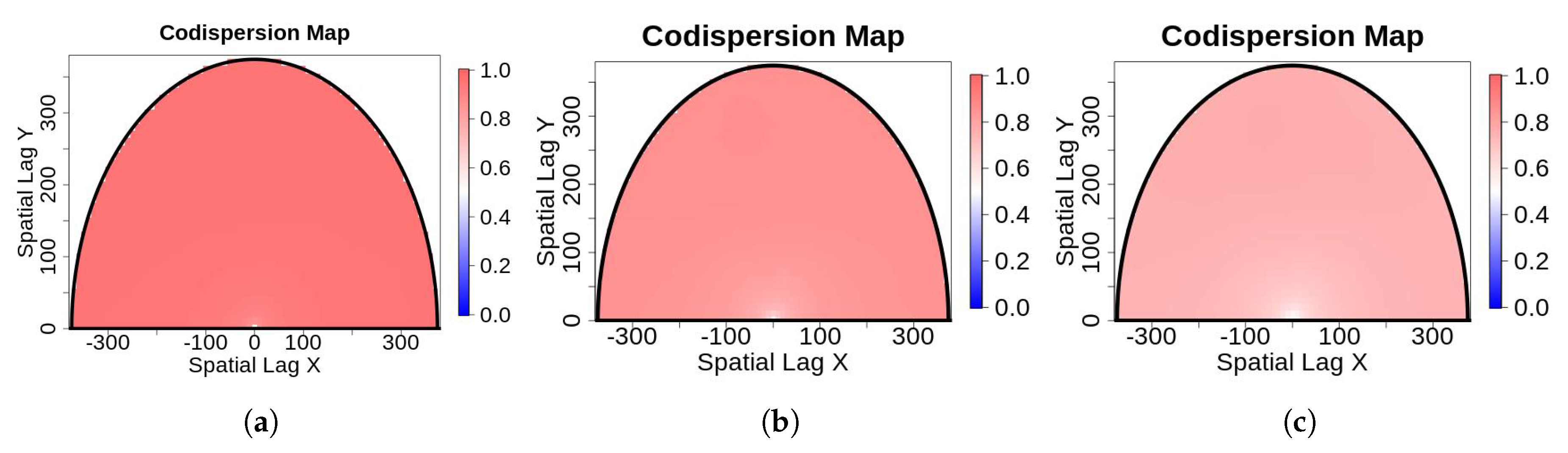
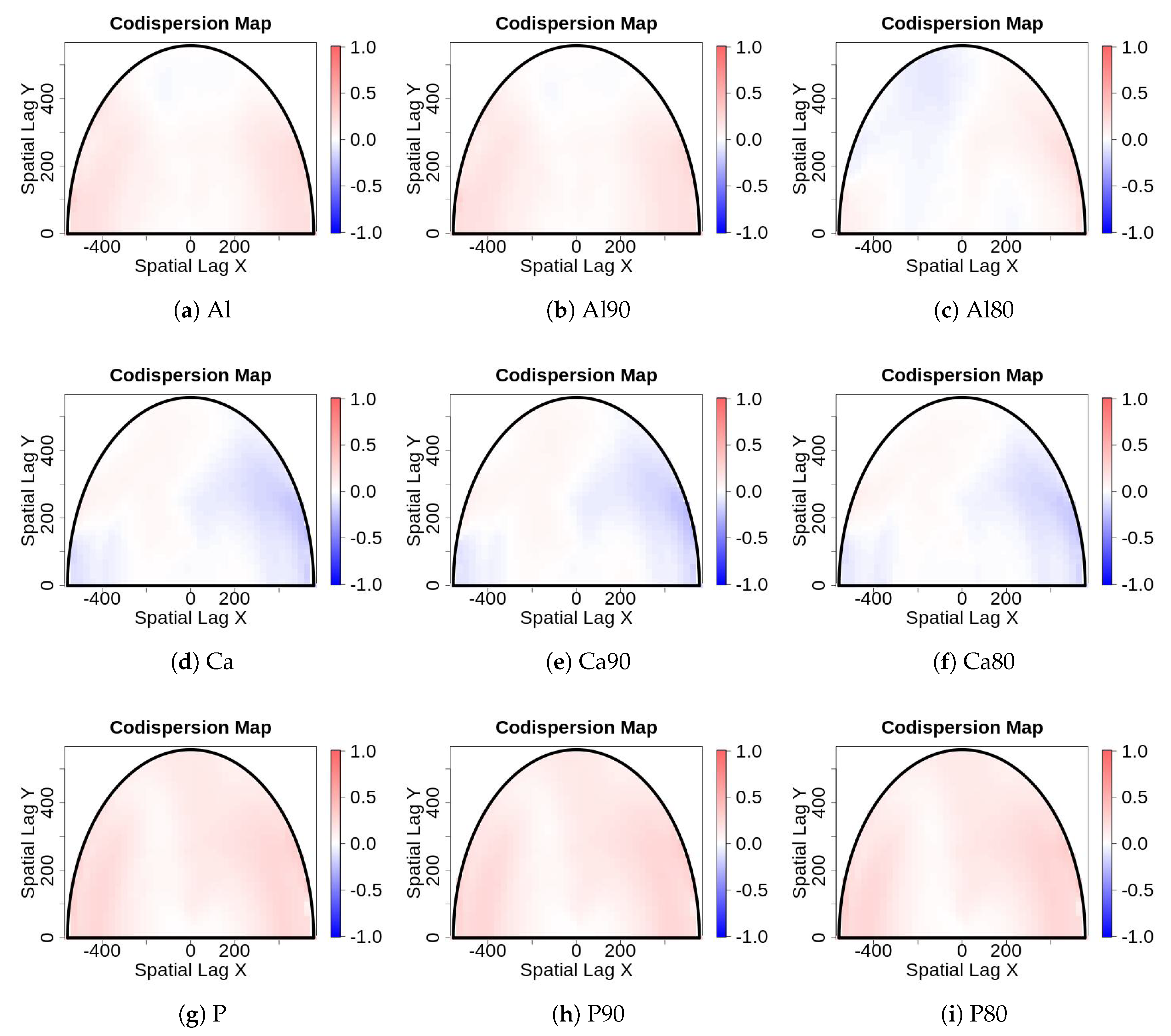
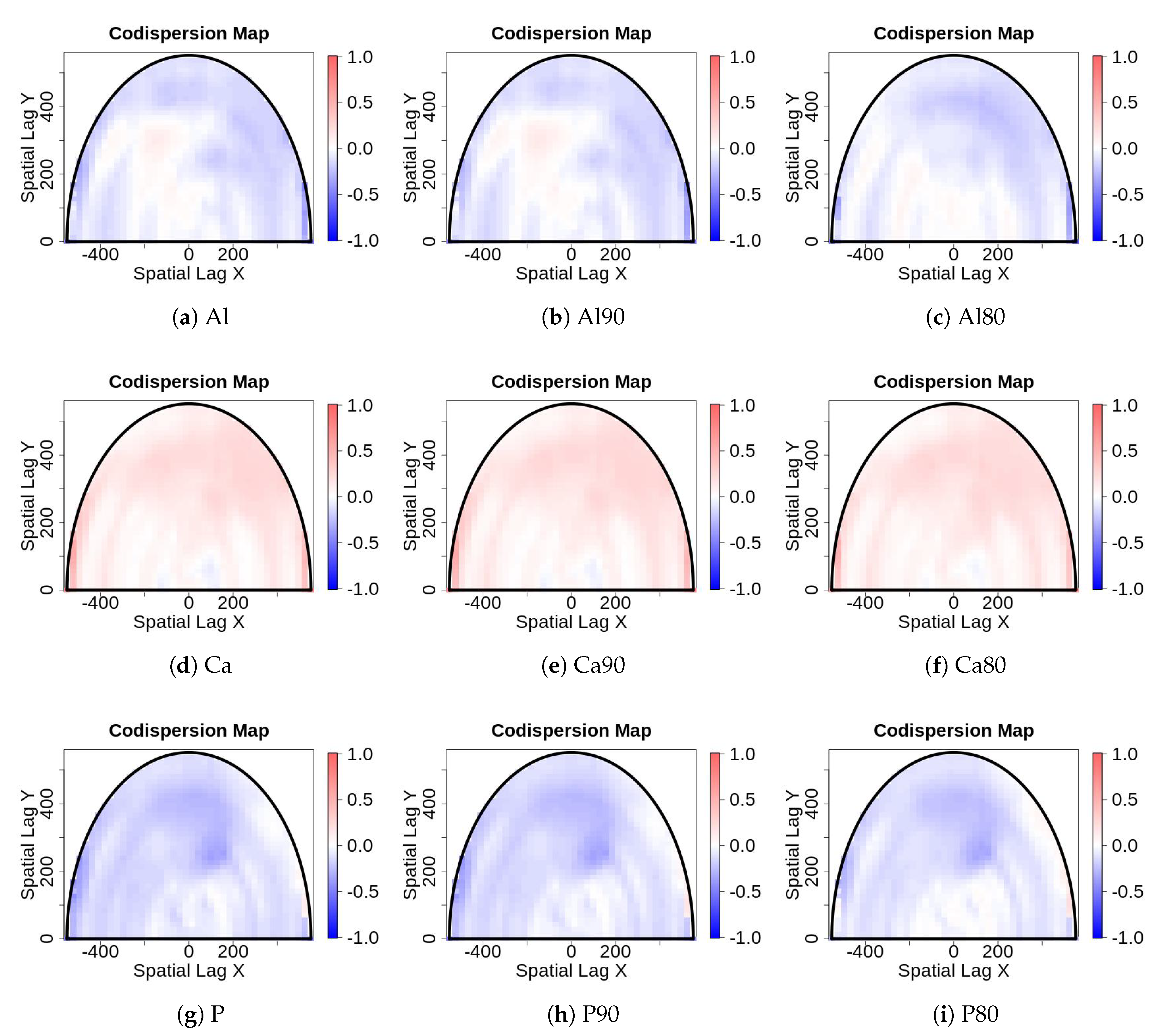
- Sampling error: Values for edaphic or environmental variables at specific locations in space often are sampled from a smoothed (kriged) surface, which itself was generated from a much smaller set of field observations. The actual information in the kriged surface is a function of both the number of observations and the smoothing parameter of the covariance function [18]. For a pair of spatial point processes and (e.g., individual forest trees and soil nutrient concentrations at each tree, respectively), where the number of observed trees (hundreds to thousands) vastly exceeds the number of soil samples (tens), we kriged the soil chemistry variables after thinning (or not) and then calculated the codispersion between the observed tree diameters and the value of the soil-chemistry variable predicted (at each tree location in ) from the kriged surface of soil-chemistry data. The kriged surface was computed either from all the data or from “thinned” soil datasets that contained 90% or 80% of the original soil chemistry data [18]. The sampling error here is error in the predicted values at points on the kriged surface caused by fitting the surface to fewer and fewer points in the “thinned” datasets.To illustrate the effect of this sampling error, we used data from plants and soils collected in the 50-ha forest dynamics plot on Barro Colorado Island, Panamá [19,20,21]. Of the 299 plant species mapped, identified, and measured every five years in this plot, we used six: Alseis blackiana, Oenocarpus mapora, Hirtella triandra, Protium tenuifolium, Poulsenia armata, and Guarea guidonia (Figure 5). The abundances of unique single-stemmed individuals of each of these six species ranged from 993 (Poulsenia armata) to 7928 (Alseis blackiana), and included species that had a range of positive, negative, and weak associations with measured soil variables [22]. Spatial locations and “diameters at breast height” (at 1.3 m aboveground) of individual trees of each species (excluding dead individuals and individuals with more than one stem) were taken from the seventh (2010) semi-decadal census of the plot.Soil samples were collected on a 50-m lattice in 2005 with additional samples taken at finer spatial grains at alternate sampling stations [22]. Soil samples were analyzed for concentrations of 11 elements; we used only data for concentrations of calcium (Ca), phosphorus (P), and aluminium (Al), as these three had the highest loadings on the first three principal axes of a multivariate analysis (NMDS) on the complete soil dataset [22]. We used ordinary kriging in the geoR package [23], version 1.7-5.2, to fit a surface to the data for each soil element and predict its concentration at the location of each tree (Figure 6). Variogram models (exponential, exponential, and wave for Ca, P, and Al, respectively) needed as input for the kriging function were fit to detrended (2nd-order polynomial) data that had been Box–Cox transformed ( = 0.5, 1.0, and 1.0 for Ca, P, and Al, respectively); kriging was done on back-transformed data to which the trend had been added. Nuggets were estimated empirically for Ca and P, but the nugget for Al was fixed (following visual inspection of the empirical variogram) equal to 4000. Alternatively, in order to take into account the spatial heterogeneity, one could perform a test to measure the degree of spatial heterogeneity along the lines given in [24], before applying the kriging interpolation.
3. Results
We used codispersion maps [3,4] to explore the possible patterns and features caused by the introduction of noise and to evaluate the performance of the codispersion coefficient when the process was contaminated with one of the distortions described above. Recall that the generation of the noise is through statistical models that do not necessarily include a particular direction in space. The effects of specific directional contamination on codispersion was investigated in [3].
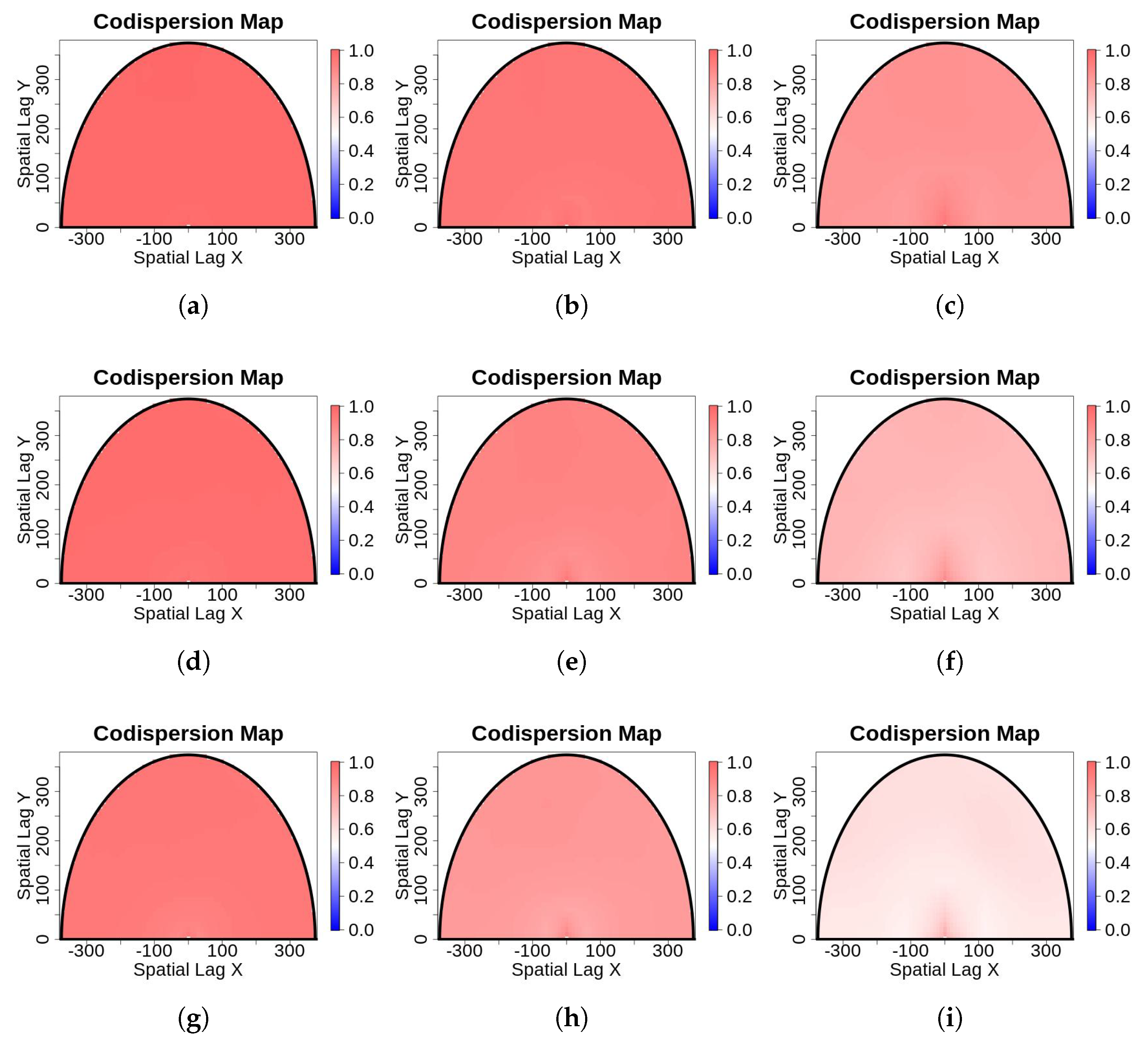
The only effect observed when the forest image was contaminated with salt-and-pepper noise (Figure 1) was a trend of decreasing codispersion between the original and contaminated images with an increase in the percentage of contamination (in Figure 7, notice a color degradation in the map as the percentage of contamination increases). In the case of the dependent processes generated by a Gaussian process with covariance matrix as in (5), we plotted the codispersion maps between the original and contaminated images displayed in Figure 2. The salt-and-pepper contamination caused a complete loss of correlation between the two images, which were originally correlated strongly (r = 0.8; Figure 8). This is in agreement with [3], who reported that visually, it is possible to observe a degradation of the original patterns as an effect of the percentage of contamination. A decrease in codispersion between the original and contaminated images was also observed when noise was introduced through missing observations at random locations or as the missing block size increased (Figure 9).
Figure 4 illustrates how we introduced large gaps of missing values in the center of the reference image shown in Figure 1a. Before computing the codispersion map, we imputed the missing data (Algorithm 2 in the Appendix A). Although the performance of such algorithms strongly depends on the size of the block of missing observations, the construction of it is based on the spatial information contained in the nearest neighbors (Algorithm 1 in the Appendix A). The spatial autoregressive lags in the AR-2D process are fixed when the order of the process is chosen. In this case, three neighbors were considered in a strongly causal set to guarantee an infinite moving average representation of the process. The images filled by the imputation algorithm are shown in Figure 10d–f. The filled areas are smooth in terms of texture and have a smaller variance. Visually, the imputation of the larger missing block looks different from the rest of the image. For small missing blocks, it is difficult to see the imputed values. From Figure 10g–h, we observed that Algorithm 2 was able to recover valuable information and that the codispersion between the original and imputed images in all cases was close to one.
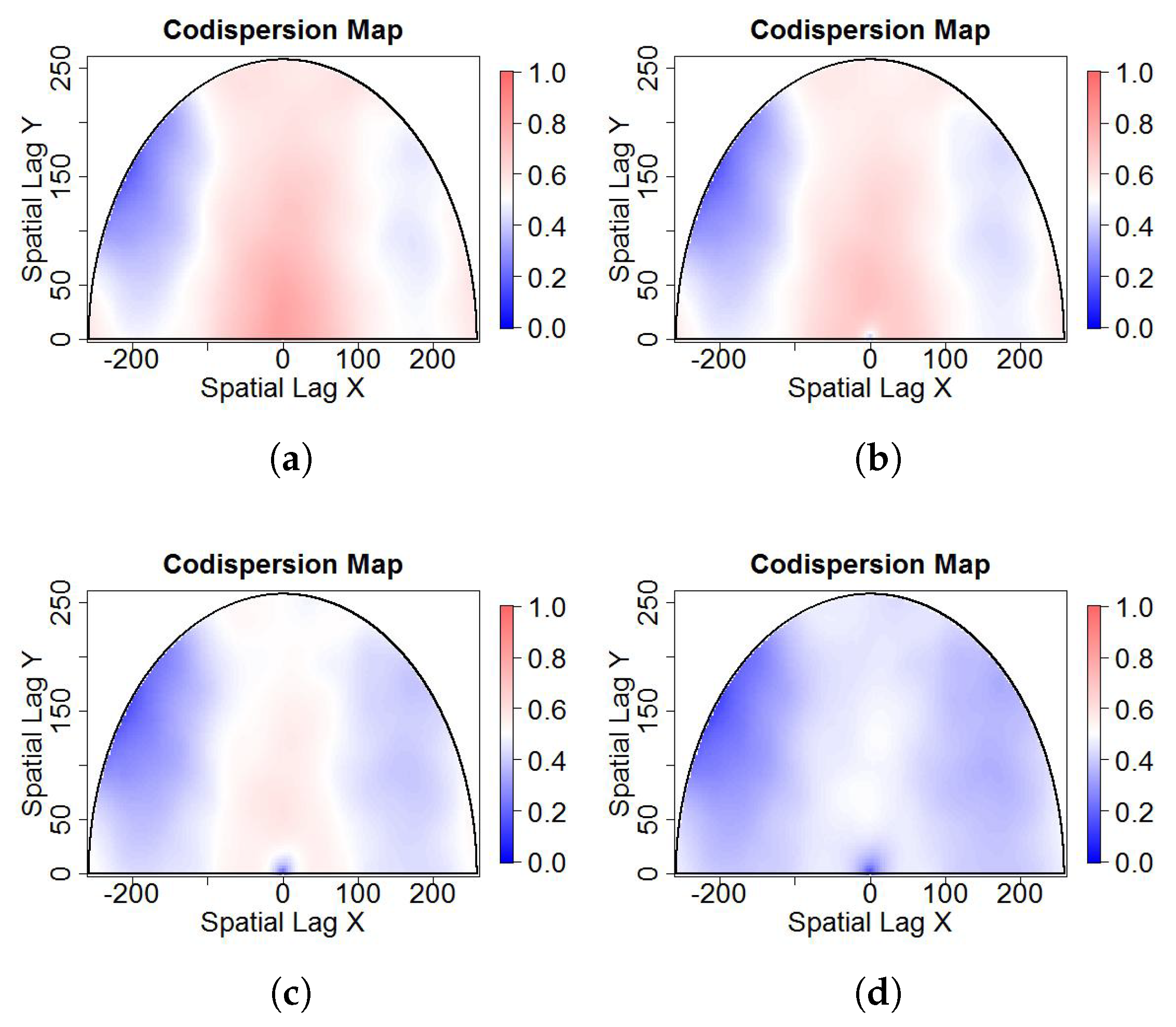
Finally, the codispersion between tree species’ diameters (for the six species shown in Figure 5) and the three soil elements (Figure 6) sampled in the Barro Colorado Island plot at three levels of data “thinning” (i.e., estimates of soil properties derived from kriged surfaces of all the soil samples, 90% of them, or 80% of them) showed that codispersion was robust to this form of error. Only the results for the most abundant (Figure 11) and the least abundant (Figure 12) species are shown.
4. Discussion
The methods and examples developed in this paper improve our understanding of the behavior of the codispersion coefficient when data are noisy or have been contaminated by various types of errors common in remotely-sensed images or in interpolated and predicted (e.g., kriged) surfaces. The codispersion coefficient appears to be robust for small percentages of contamination (<15%) but always leads to an underestimation of the codispersion between the datasets. As the percentage of contamination increases, codispersion decreases uniformly for all directions on the plane, thus the types of noise considered in this paper did not affect the codispersion in any particular direction(s). Although the performance of codispersion for directional noise was explored in [3,25], directional noise has not yet been observed in real datasets.
When applied to data collected from large forest plots, codispersion has been shown to be useful for describing scales of covariation in two or more variables across complex spatial gradients (e.g., [4,5]). Our ability to detect such spatial pattern depends on the grain of spatial variation in the data and how this compares to the lag sizes used in the codispersion analysis. For example, the complete loss of correlation between the two images in Figure 2 with only a small degree of contamination highlights the importance of considering the spatial grain of the datasets relative to that of the noise-inducing processes. The coarser-grained spatial pattern in the forest images is retained, even under contamination, whereas the spatial dependence in the images in Figure 2 is at a smaller grain than the extent of the image, which is relatively heavily disturbed by the salt-and-pepper noise.
The imputation algorithm described in Appendix A seems to be a promising technique to handle blocks of missing observations. Several aspects of it are worth exploring with future research. These include the success of the algorithm in recovering missing observations as a function of the block size; how to select the number of neighbors to be considered in the AR-2D process; and the similarity between the texture of the imputed observations and the texture of the reference image. For simplicity and without loss of generality, the missing blocks we illustrated were square regions located in the center of the image, but certainly Algorithm 2 could be extended to other types of regions located anywhere in the image.
More general aspects of codispersion analysis are in need of further exploration and testing. First, it will be of interest to study the results of codispersion analysis of rasterized images. This is because rasterization of images is widespread and common rasterization methods rarely, if ever, preserve the original spatial correlation of each process. The development of a new rasterization method that preserves better the spatial correlation within processes could follow [26]. Second, the computation of codispersion maps is computationally expensive. Thus, the development of efficient algorithms capable of creating codispersion maps for large images is still needed.
5. Conclusions
The codispersion map is a useful tool that illustrates those directions for which the codispersion coefficient between two spatial processes attains its maximum and minimum values. When the direction of interest in unknown, the codispersion map also visually and concisely summarizes the correlation between two processes in a plane. When data are noisy or have some degree of observation or process error our results suggest that:
- (1)
- The codispersion coefficient is robust to small percentages of contamination (less than 15%).
- (2)
- The codispersion coefficient decreases as the percentage of contamination increases no matter the type of noise or direction.
- (3)
- For data collected from large forest plots, the codispersion coefficient and the associated codispersion map provide useful information to describe covariation in the data across complex spatial gradients or patterns.
- (4)
- An imputation algorithm can be used to smoothly fill blocks of missing observations with little impact on the codispersion coefficient.
The development of codispersion maps for large data sets can be addressed by using the effective sample size for spatial variables, recently proposed in [27].
Supplementary Materials
Analyses were done using the R software system, version 3.3.1 [28]. The images and all the code used in this paper are available from https://github.com/JAcostaS/Code-and-Example-Codismap.git. Barro Colorado Island (BCI) vegetation and soils data are available from http://ctfs.si.edu/webatlas/datasets/bci/.
Author Contributions
R.V. developed the theoretical formalism of the codispersion map, J.A. worked on the computational aspects related to the construction of the codispersion map and the imputation algorithm. H.B. and B.C. performed the numeric calculations and the display of the example related with individual forest trees and soil nutrient concentrations. A.M.E. conceived this research, plan the structure of the paper and selected the appropriate real examples. All authors wrote parts of the paper, provided critical feedback and helped shape the research, analysis and manuscript.
Funding
This research was funded by AC3E, grant number FB-0008, Chile.
Acknowledgments
R.V. was partially supported by AC3E, FB-0008, Valparaíso, Chile. J.A. was supported by Pontificia Universidad Católica de Valparaíso, Grant 039.320/2018. A.M.E.’s participation in this project was supported by Harvard University and the Universidad Técnica Federico Santa María, and Hannah Buckley. and Bradley Case’s work on this project in Chile also was supported by the Universidad Técnica Federico Santa María. Vegetation data from BCI are part of the BCI forest dynamics research project founded by S. P. Hubbell and R. B. Foster and now managed by R. Condit, S. Lao, and R. Perez through the Center for Tropical Forest Science (CTFS) and the Smithsonian Tropical Research Institute (STRI) in Panamá. Numerous organizations have provided funding to support this long-term study, principally the US National Science Foundation (NSF), and hundreds of field workers have contributed to mapping, measuring and monitoring the vegetation. Jim Dalling, Robert John, Kyle Harms, Robert Stallard, Joe Yavitt, Paolo Segre, and Juan Di Trani sampled the soils at BCI. Collection and initial analysis of the BCI data were supported by NSF grants 021104, 021115, 0212284, 0212818 and 0314581, the STRI Soils Initiative, and CTFS. This paper is a publication of the Harvard Forest Long-Term Ecological Research Site, supported by the US National Science Foundation.
Conflicts of Interest
The authors declare no conflict of interest.
Appendix A. Image Imputation Algorithm
The algorithm described below is based on the fact that it is possible to represent any image by using unilateral AR-2D processes [17,29]. The generated image is called a local AR-2D approximated image by using blocks.
Let be an original image, and let X the original image corrected by the mean. That is, for all and for which is the mean of Z.
Following [30], assume that X follows a causal AR-2D process of the form
where , is Gaussian white noise, and , and are the autoregressive parameters.
Let For simplicity, we consider that the images to be processed are arranged in such a way that the number of columns minus one and the number of rows minus one are multiples of ; Then, we define the block of the image X by
for all and for all , where denotes the integer part. The approximated image , where and can be obtained by the following algorithm.
| Algorithm 1 Approximated AR-2D Image. |
| Input: An original image Z of size . Output: An approximated of size
|
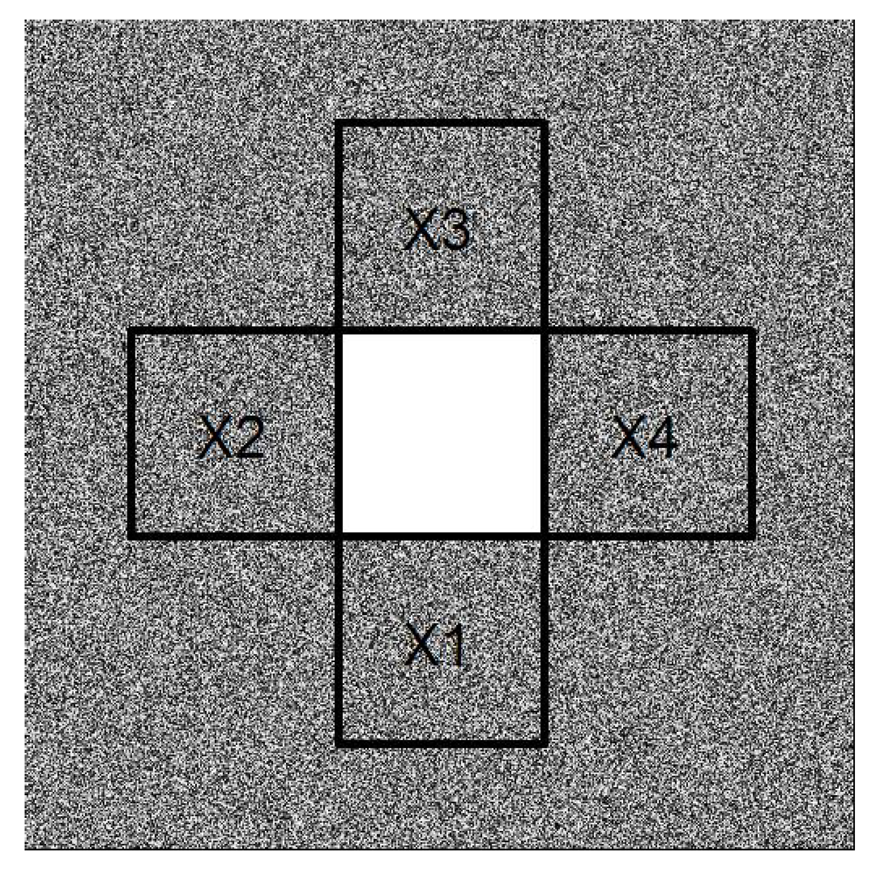
Now suppose that image Z has a rectangular block of missing values. Without loss of generality, assume that the rectangular block of missing values is of size . Furthermore, in each border, , , is defined as a block of information of Z of size , such as appears in Figure A1.
Figure A1.
Block of missing values.

In addition, assume that all l, are represented by a AR-2D model of the form
where , , and are estimated using the block for , respectively. Then, the prediction model is
where is the index set for which is known and . The prediction algorithm is the following.
| Algorithm 2 Prediction Algorithm. |
| Input: An image Z with a missing block, and K. Output: Image Z without missing values.
|
References
- Fortin, M.J.; Dale, M. Spatial Analysis: A Guide for Ecologists; Cambridge University Press: Cambridge, UK, 2005; pp. 5–11. [Google Scholar]
- Ellison, A.M.; Gotelli, N.J.; Hsiang, N.; Lavine, M.; Maidman, A. Kernel density estimation of 2-dimensional spatial Poisson point processes from k-tree sampling. J. Agric. Biol. Environ. Stat. 2014, 19, 357–372. [Google Scholar] [CrossRef] [Green Version]
- Vallejos, R.; Osorio, F.; Mancilla, D. The codispersion map: A graphical tool to visualize the association between two spatial processes. Stat. Neerl. 2015, 69, 298–314. [Google Scholar] [CrossRef]
- Buckley, H.L.; Case, B.S.; Ellison, A.M. Using codispersion analysis to characterize spatial patterns in species co-occurrences. Ecology 2016, 97, 32–39. [Google Scholar] [CrossRef] [PubMed] [Green Version]
- Buckley, H.L.; Case, B.S.; Zimmermann, J.; Thompson, J.; Myers, J.A.; Ellison, A.M. Using codispersion analysis to quantify and understand spatial patterns in species-environment relationships. New Phytol. 2016, 211, 735–749. [Google Scholar] [CrossRef] [PubMed] [Green Version]
- Case, B.S.; Buckley, H.L.; Barker Plotkin, A.; Ellison, A.M. Using codispersion analysis to quantify temporal changes in the spatial pattern of forest stand structure. Chil. J. Stat. 2016, 7, 3–15. [Google Scholar]
- Ellison, A.M.; Osterweil, L.J.; Hadley, J.L.; Wise, A.; Boose, E.; Clarke, L.; Foster, D.R.; HAnson, A.; Jensen, D.; Kuzeja, P.; et al. Analytic webs support the synthesis of ecological datasets. Ecology 2006, 87, 1345–1358. [Google Scholar] [CrossRef]
- Matheron, G. Les Variables Régionalisées et leur Estimation; Masson: Paris, France, 1965. [Google Scholar]
- Ojeda, S.; Vallejos, R.; Lamberti, P. Measure of similarity between images based on the codispersion coefficient. J. Electron. Imaging 2012, 21, 023019. [Google Scholar] [CrossRef]
- Anselin, L. Local indicators of spatial association–LISA. Geogr. Anal. 1995, 27, 93–115. [Google Scholar] [CrossRef]
- Fox, A.J. Outliers in time series. J. R. Stat. Soc. B 1972, 34, 350–363. [Google Scholar]
- Huang, S.; Zhu, J. Removal of salt-and-pepper noise based on compressed sensing. Electron. Lett. 2010, 46, 1198–1199. [Google Scholar] [CrossRef]
- McQuarrie, A.D.; Tsai, C. Outlier detections in autoregressive models. J. Comput. Graph. Stat. 2003, 12, 450–471. [Google Scholar] [CrossRef]
- Gneiting, T.; Kleiber, W.; Schlather, M. Matérn cross-covariance functions for multivariate random fields. J. Am. Stat. Assoc. 2010, 105, 1167–1177. [Google Scholar] [CrossRef]
- Schlather, M.; Malinowski, A.; Oesting, M.; Boecker, D.; Strokorb, K.; Engelke, S.; Martini, J.; Ballani, F.; Moreva, O.; Auel, J.; et al. RandomFields: Simulation and Analysis of Random Fields. R Package Version 3.1.50. 2017. Available online: https://cran.r-project.org/package=RandomFields (accessed on 1 April 2018).
- Allende, H.; Galbiati, J.; Vallejos, R. Robust image modeling on image processing. Pattern Recognit. Lett. 2001, 22, 1219–1231. [Google Scholar] [CrossRef]
- Ojeda, S.; Vallejos, R.; Bustos, O. A new image segmentation algorithm with applications to image inpainting. Comput. Stat. Data Anal. 2010, 54, 2082–2093. [Google Scholar] [CrossRef]
- Minasny, B.; McBratney, A.B. The Matérn function as a general model for soil variograms. Geoderma 2005, 128, 192–207. [Google Scholar] [CrossRef]
- Condit, R. Tropical Forest Census Plots; Springer: Berlin, Germany, 1998. [Google Scholar]
- Hubbell, S.P.; Condit, R.; Foster, R.B. Barro Colorado Forest Census Plot Data. 2005. Available online: http://ctfs.si.edu/webatlas/datasets/bci (accessed on 18 February 2018).
- Hubbell, S.P.; Foster, R.B.; O’Brien, S.T.; Harms, K.E.; Condit, R.; Wechsler, B.; Wright, S.J.; Loo de Lao, S. Light gap disturbances, recruitment limitation, and tree diversity in a neotropical forest. Science 1998, 283, 554–557. [Google Scholar] [CrossRef]
- John, R.; Dalling, J.W.; Harms, K.E.; Yavitt, J.B.; Stallard, R.F.; Mirabello, M.; Hubbell, S.P.; Valencia, R.; Navarrete, H.; Vallejo, M.; et al. Soil nutrients influence spatial distributions of tropical trees. Proc. Natl. Acad. Sci. USA 2007, 104, 864–869. [Google Scholar] [CrossRef]
- Ribeiro, P.J., Jr.; Diggle, P.J. geoR: A package for geostatistical analysis. R-News 2001, 1, 15–18. [Google Scholar]
- Wang, J.-F.; Zhang, T.-L.; Fu, B.-J. A measure of spatial stratified heterogeneity. Ecol. Indic. 2016, 67, 250–256. [Google Scholar] [CrossRef] [Green Version]
- Vallejos, R.; Mancilla, D.; Acosta, J. Image similarity assessment based on measures of spatial association. J. Math. Imaging Vis. 2016, 56, 77–98. [Google Scholar] [CrossRef]
- Goovaerts, P. Combining Areal and Point Data in Geostatistical Interpolation: Applications to Soil Science and Medical Geography. Math. Geosci. 2010, 42, 535–554. [Google Scholar] [CrossRef] [PubMed] [Green Version]
- Acosta, J.; Vallejos, R. Effective sample size for spatial regression processes. Electron. J. Stat. 2018, 12, 3147–3180. [Google Scholar] [CrossRef]
- R Development Core Team. R: A Language and Environment for Statistical Computing; R Foundation for Statistical Computing: Vienna, Austria, 2016; Available online: http://www.R-project.org (accessed on 22 March 2018).
- Ver Hoef, J.M.; Peterson, E.E.; Hooten, M.B.; Hanks, E.M.; Fortin, M.J. Spatial autoregressive models for statistical inference from ecological data. Ecol. Monogr. 2018, 88, 36–59. [Google Scholar] [CrossRef] [Green Version]
- Bustos, O.; Ojeda, S.; Vallejos, R. Spatial ARMA models and its applications to image filtering. Braz. J. Prob. Stat. 2009, 23, 141–165. [Google Scholar] [CrossRef]
Figure 1.
(a) reference image of size pixels taken above a section of forest at the Harvard Forest, Petersham, MA, USA and (b) its corresponding gray scale values. (c,e,g) are the same image distorted with increasing amounts of salt-and-pepper noise. The percentages of contamination are 5%, 10%, and 25%, respectively; (d,f,h) show the change in gray intensity after the addition of salt-and-pepper noise to the images.

Figure 2.
Images (a,b) are dependent processes generated from a Gaussian process with a covariance matrix as in (5); (c–e) salt and pepper contamination of (b) considering , and , , , and in each case, where is the size of the image.
Figure 2.
Images (a,b) are dependent processes generated from a Gaussian process with a covariance matrix as in (5); (c–e) salt and pepper contamination of (b) considering , and , , , and in each case, where is the size of the image.

Figure 3.
Contamination of of the reference image shown in Figure 1a by salt and pepper at random locations. The missing blocks are of size , , and , respectively, shown in the different columns. (a–c): the proportion of missing blocks is 0.000002; (d–f): the proportion of missing blocks is 0.000004; (d–f): the proportion of missing blocks is 0.000008.

Figure 4.
Gaps of missing observations of sizes (a); (b); and (c).

Figure 5.
Distribution and size of the six species of trees growing in the 50-hectare plot at Barro Colorado Island, Panamá that we analyzed to assess the effect of sampling error.
Figure 5.
Distribution and size of the six species of trees growing in the 50-hectare plot at Barro Colorado Island, Panamá that we analyzed to assess the effect of sampling error.

Figure 6.
Kriged surfaces of the concentration (mg/kg) of aluminum (Al; top), calcium (Ca; center), and phosphorus (P; bottom) in the 50-hectare plot at Barro Colorado Island, Panamá. Contours were estimated for a regular grid (5-m spacing) based on data from samples taken at approximately 50-m intervals. Interpolated values of mineral concentrations were estimated at individual points (locations of trees) shown on the plots.

Figure 7.
Codispersion map between (a) the original Figure 1a,c (5%); (b) the original Figure 1a,e (15%); (c) the original Figure 1a,g (25%).

Figure 8.
Images (a–d) are the corresponding codispersion maps between Figure 2a and the contaminated Figure 2b–e.

Figure 9.
Codispersion map between the reference Figure 1a and the images contaminates with missing observation at random locations depicted in Figure 3a–i. Images (a)–(i) show how the correlation decreases when the missing block size increases.

Figure 10.
Contamination of the reference Figure 1a by gaps resulting from clusters of missing observations. Images (a–c) contain only one missing block in the center of the image of sizes , , y , respectively. These missing data were filled in images (d–f) using the imputation algorithm described in the Appendix. Images (g–l) are the corresponding codispersion maps between Figure 1a and the imputed images (d–f).

Figure 11.
Codispersion between species A. blackiana and soil chemistry variables; (Al (a–c); Ca (d–f) and P (g–i)). Soil data were unthinned (a,d,g); thinned 10% (b,e,h); or thinned 20% (c,f,i).
Figure 11.
Codispersion between species A. blackiana and soil chemistry variables; (Al (a–c); Ca (d–f) and P (g–i)). Soil data were unthinned (a,d,g); thinned 10% (b,e,h); or thinned 20% (c,f,i).

Figure 12.
Codispersion between species P. armata and soil chemistry variables; (Al (a–c); Ca (d–f) and P (g–i)). Soils data were unthinned (a,d,g), thinned 10% (b,e,h), or thinned 20% (c,f,i).
Figure 12.
Codispersion between species P. armata and soil chemistry variables; (Al (a–c); Ca (d–f) and P (g–i)). Soils data were unthinned (a,d,g), thinned 10% (b,e,h), or thinned 20% (c,f,i).

© 2018 by the authors. Licensee MDPI, Basel, Switzerland. This article is an open access article distributed under the terms and conditions of the Creative Commons Attribution (CC BY) license (http://creativecommons.org/licenses/by/4.0/).
Share and Cite
MDPI and ACS Style
Vallejos, R.; Buckley, H.; Case, B.; Acosta, J.; Ellison, A.M. Sensitivity of Codispersion to Noise and Error in Ecological and Environmental Data. Forests 2018, 9, 679. https://doi.org/10.3390/f9110679
AMA Style
Vallejos R, Buckley H, Case B, Acosta J, Ellison AM. Sensitivity of Codispersion to Noise and Error in Ecological and Environmental Data. Forests. 2018; 9(11):679. https://doi.org/10.3390/f9110679
Chicago/Turabian StyleVallejos, Ronny, Hannah Buckley, Bradley Case, Jonathan Acosta, and Aaron M. Ellison. 2018. "Sensitivity of Codispersion to Noise and Error in Ecological and Environmental Data" Forests 9, no. 11: 679. https://doi.org/10.3390/f9110679
Note that from the first issue of 2016, this journal uses article numbers instead of page numbers. See further details here.