Spatial and Temporal Patterns in Nonstationary Flood Frequency across a Forest Watershed: Linkage with Rainfall and Land Use Types

1
School of Water Conservancy, North China University of Water Resources and Electric Power, Zhengzhou 450046, China
2
Jiangxi Provincial Key Laboratory of Soil Erosion and Prevention, Nanchang 330029, China
3
Jiangxi Institute of Soil and Water Conservation, Nanchang 330029, China
4
College of Resources and Environment, Huazhong Agricultural University, Wuhan 430070, China
5
Henan Yellow River Hydrological Survey and Design Institute, Zhenghzou 450002, China
6
Collaborative Innovation Center of Water Resources Efficient Utilization and Support Engineering, Zhengzhou 450046, China
*
Author to whom correspondence should be addressed.
Forests 2018, 9(6), 339; https://doi.org/10.3390/f9060339
Submission received: 10 April 2018
/
Revised: 3 June 2018
/
Accepted: 6 June 2018
/
Published: 8 June 2018
(This article belongs to the Special Issue Forest Hydrology and Watershed)
Abstract
:Understanding the response of flood frequency to impact factors could help water resource managers make better decisions. This study applied an integrated approach of a hydrological model and partial least squares (PLS) regression to quantify the influences of rainfall and forest landscape on flood frequency dynamics in the Upper Honganjian watershed (981 km2) in China. The flood events of flood seasons in return periods from two to 100 years, wet seasons in return periods from two to 20 years, and dry seasons in return periods from two to five years show similar dynamics. Our study suggests that rainfall and the forest landscape are pivotal factors triggering flood event alterations in lower return periods, that flood event dynamics in higher return periods are attributed to hydrological regulations of water infrastructures, and that the influence of rainfall on flood events is much greater than that of land use in the dry season. This effective and simple approach could be applied to a variety of other watersheds for which a digital spatial database is available, hydrological data are lacking, and the hydroclimate context is variable.
1. Introduction
Flood frequency is the probability of a flood event in a certain period, which is relevant to planning and decision processes related to hydraulic works or flood alleviation programs [1]. Thorough knowledge of flood frequency dynamics is crucial in a watershed [2,3,4]. Variations in flood frequencies result from meteorological factors and underlying surface properties, including rainfall, flood control facilities, topography, soil and land use types [3,5]. Among these factors, flood control facilities represent passive defense structures against floods; topography and soil are relatively constant in short periods, whereas rainfall and land use are variable [3,5,6,7,8]. Therefore, determining the response of flood frequencies to rainfall and land use is crucial for water resource management in watersheds [5,9]. However, major challenges are associated with flood frequency response research, including failed estimation of flood frequencies, lack of data, and the high collinearity of rainfall and land use types [8,10].
To quantify the factors controlling flood frequency, estimation for flood frequencies is a prerequisite. Frequency analysis (FA) is a method used to fit the frequency of extreme hydrological events to their magnitudes by using probability distributions [6,10,11]. FA has played an important role in increasing the prediction accuracy of flood frequencies [2,10,11]. Other methods, such as empirical relationships and the fuzzy logic approach, have also been applied to a few watersheds [10]. Many FA methods have been developed and tested, including the index flood method, the rational method, and various regression-based methods [2]. The disadvantages of conventional FA could be the significant uncertainties and bias, which are due to limited historical recorded data with sufficient spatial and temporal coverage and acceptable quality, sampling variability, model errors, and the errors in projections into the future [12,13]. In addition, this traditional technology is based on the assumption that the hydrological observations are independently and identically distributed and the conditions remain stationary [11,14]. Lastly, FA focuses on flood peak values; however, the severity of a flood is defined not only by the flood peak value but also by flood volume, duration, etc. [15]. In practical applications, the flood series are always not independent and exist in a nonstationary context, and the watershed always contains a large number of ungauged areas [16]. Overall, conventional FA provides a limited assessment of flood frequencies [14]. Using conventional FA on nonstationary flow series may lead to uncertain flood frequency predictions [11,17].
To overcome these limitations, a nonstationary FA framework combined with lognormal or generalized extreme value distribution models and hydrological models has been developed [5,18]. Nonstationary FA coupled probability distribution has been considered an effective improvement in flood frequency analysis, with observations that are not independent under nonstationary circumstances [2,11,14]. To address these challenges of data scarcity, hydrological models have the ability to complement available datasets from local gauging stations with a spatial extension. This modeling approach provides some advantages: (1) planned alterations in rainfall and land use can be considered, and hydrological modeling allows one to obtain the full hydrograph for the design, and (2) the estimation of design flows can be performed for ungauged watersheds if the parameters of the hydrological model are regionalized [4]. Recently, many studies have reported the use of hydrological models, such as the HECHMS, WRF/DHSVM, and SWAT models, to simulate floods [4,17,19]. The SWAT model can divide a watershed into sub-watersheds and then discretize them into a series of hydrologic response units (HRUs), which are spatially identified as unique soil–land use combination areas. SWAT can also provide a wide range of flexibility for model formulation and calibration [20,21,22]. A nonstationary FA framework incorporated with SWAT is a relatively new modeling approach and has been shown to provide acceptable prediction results when the hydroclimate context is variable, data are lacking, or the spatiotemporal analysis is complex [20,21,23].
Multivariate regression approaches have great potential for quantifying the relative importance of rainfall and land use types in controlling flood frequencies. However, traditional multivariate approaches cannot easily overcome the limitations of rainfall and land use types, which are highly collinear predictors [8,22,24,25]. Therefore, non-independent data must be handled cautiously in quantitative analyses. Partial least squares (PLS) regression is an advanced method that combines the features of principal component analysis and multiple linear regressions. It has been widely used to overcome the issue of multicollinearity and noisy data in quantitative analyses by projecting variables on high-dimensional spaces [26]. The importance of a predictor to variations in model fitting is given by the variable influence on projection (VIP) value. VIP values reflect the importance of terms in a model with respect to both Y, i.e., a variable’s correlation to all responses, and X, i.e., the projection [27]. Variations with higher VIP values are considered more important [28]. PLS regression can be used to evaluate rainfall, forest, and other land use influences on flood events [8,22,26].
The objective of this paper is to study the influences of forest land use and precipitation on flood frequencies in the Upper Honganjian watershed in China. This investigation is separated into two parts: (1) revealing flood frequency destruction based on a nonstationary FA method and SWAT model, and (2) illuminating the response of flood frequency distribution to land use and precipitation based on PLS regression.
2. Materials and Methods
2.1. Study Area
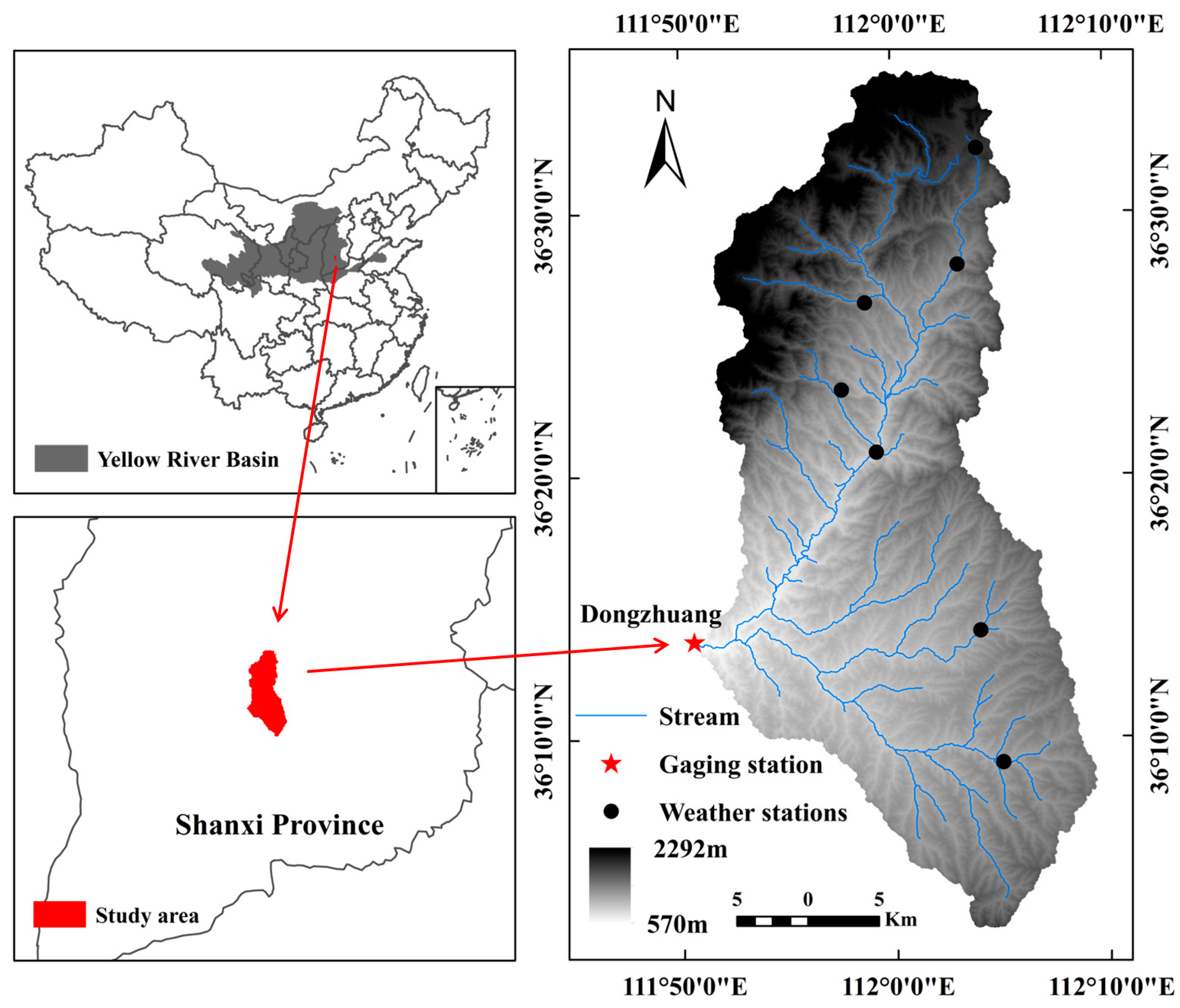
The Upper Honganjian watershed, with a total area of 981 km2, is located in the Yellow River Basin and lies between 36°2′ N to 36°34′ N and 110°50′ E to 112°10′ E. The average annual temperature is approximately 11.8 °C, and the average annual precipitation is approximately 558.5 mm. A large portion of precipitation occurs during the monsoon season from May to October. Floods occur primarily in July, August, and September [29]. The topography of the watershed is undulating and characterized by mountain ranges, steep slopes, and deep valleys. The elevation varies from 572 m at the Dongzhuang gauging station to 2259 m at the highest point in the watershed (Figure 1). The main soil types are yellow loamy soil (50.3%) and brown soil (18.8%), which correspond to Alfisols and Entisols in the USA Soil Taxonomy [30], respectively. Most areas are covered by forest (43.4%) and farmland (34.3%).
2.2. Data Collection and Pretreatment
Hydrometeorological data: Forty-six years (1965–2010) of daily streamflow data were collected at the Dongzhuang station (the outlet of the Upper Honganjian watershed). Daily precipitation, solar radiation, wind speed, relative humidity, and max/min temperatures were attained from six weather stations (Figure 1). To account for seasonal variations, the streamflow data series were split into a wet season (i.e., May, June, and October), a flood season (i.e., July–September), and a dry season (i.e., November–April). The precipitation data were interpolated over the delineated sub-watersheds using a skewed normal distribution.
Topographical and soil coverage data for the model setup: The topographical data required by the SWAT model were derived from a digital elevation model (DEM) with a resolution of 25 × 25 m, which was obtained from the National Geomatics Center of China. The soil data, including a soil type map (1:100,000) and information on the related soil properties, were obtained from the Hydrological Bureau of Shanxi Province.
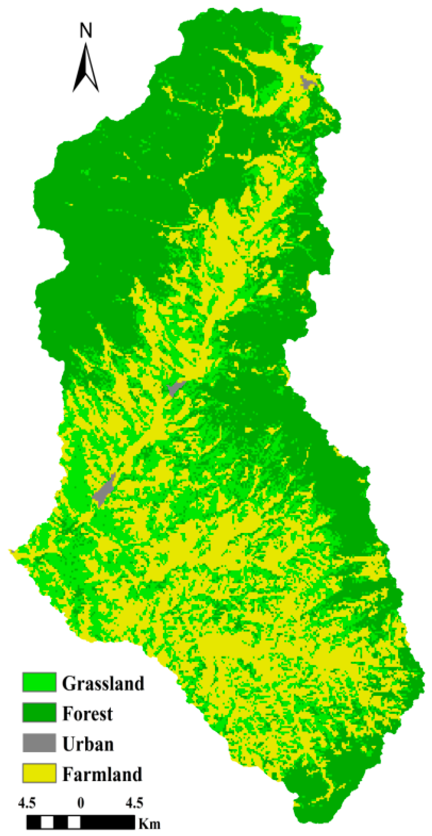
Land use data: The land use data for the 1980s were obtained from the Hydrological Bureau of Shanxi Province. Four land use domains were identified, namely, forest, farmland, urban, and grassland (Figure 2). Land use and soil data were extracted using ArcGIS Version 10.2. (Esri, Redlands, CA, USA).
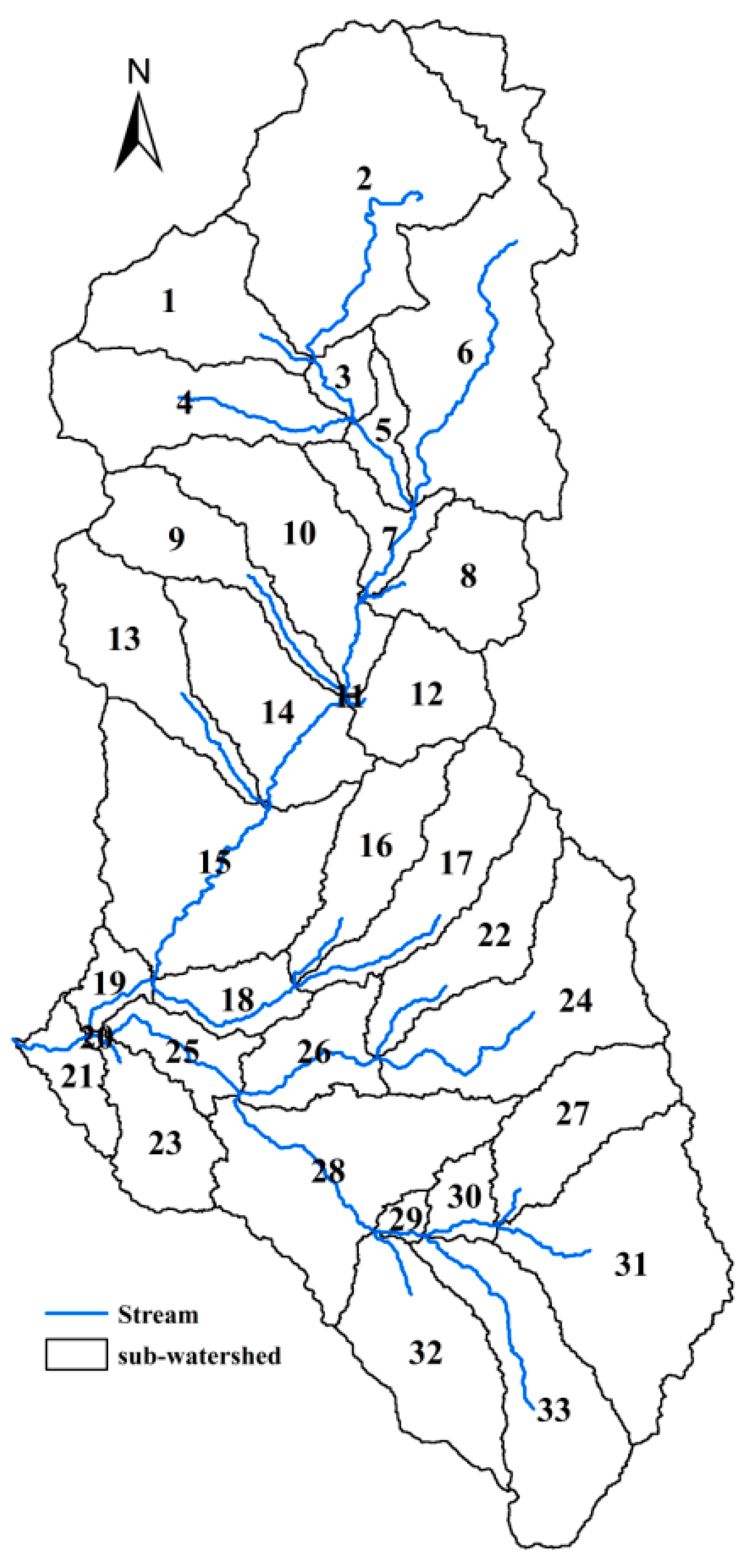
Sub-watersheds and HRUs: In ArcSWAT 2012 (Esri, Redlands, CA, USA), the Upper Honganjian watershed was discretized into 33 sub-watersheds (Figure 3), which were then further subdivided into 207 HRUs based on land use, soil, and slopes.
2.3. SWAT Model Calibration for Ungauged Sub-Watershed Streamflow
Before using the SWAT model to predict the streamflow in ungauged sub-watersheds, calibration and validation of the model were performed. Calibration was performed with automated and manual techniques. The first step in the calibration process was determination of the most sensitive parameters for studying the watershed. Sensitivity analysis of the parameters in the SWAT model was performed using the LH–OAT analysis method, which combines the Latin hypercube (LH) sampling method and the one-factor-at-a-time (OAT) sensitivity analysis method. After 350 runs, the most sensitive parameters were detected. Autocalibration was the second step. This procedure was based on shuffled complex evolution (SCE–UA), which allows calibration of model parameters based on a single objective function [31]. In the last step, the SWAT model was manually calibrated against monthly and daily streamflow data, which were observed at the Dongzhuang gauge station. The calibration period was from January 1972 to December 1981. Manual calibration was performed to minimize total flow (minimized average annual percent bias), accompanied by visual inspection of the hydrographs. The parameters governing the surface runoff response were first calibrated, followed by those governing the fraction of streamflow that transform to baseflow. This preliminary calibration was followed by a fine-tuning at the daily time scale to ensure that the predicted versus measured peak flows and recession curves on a daily time step matched as closely as possible.
The validation period was from January 1982 to December 1991. Nash–Sutcliffe efficiency (ENS), percent bias (PBIAS), and coefficient of determination (R2) were used to evaluate the performance of the model. ENS was calculated as follows [8,32]:
where n is the discrete time step and Oi and Si are the measured and simulated values, respectively. PBIAS is defined as follows [8,32]:
where Oi and Si are the measured and simulated values, respectively, and n is the total number of paired values. R2 was calculated as follows [8,32]:
where n is the number of events, Oi and Si are the measured and simulated streamflow values, respectively, and O and S are the mean observed and simulated values, respectively. The performance of the SWAT model (1) is considered acceptable when R2 and ENS are greater than 0.5 and PBIAS ranges from ±15% to ±25%; (2) is good when R2 is greater than 0.5, ENS is greater than 0.65, and PBIAS ranges from ±10% to ±15%; and (3) is very good when R2 is greater than 0.5, ENS is greater than 0.75, and PBIAS is smaller than ±10% [8,32].
2.4. Evaluation of the Quantiles of Maximum Streamflow
Based on previous studies, the annual maximum (AM) series model was used in the multistep nonstationary FA in this study [2,18]. The AM model is a framework that uses annual maximum values as appropriate estimators with a preferred distribution [10]. First, the AM series model was applied to identify the annual seasonal extreme streamflow. To identify the low and high outliers for the flow series, the Grubbs and Beck (1972) statistical test (see Appendix A.1. for more technical details) was used after the data were transformed to be normally distributed [33]. Second, to perform FA, several statistical tests were used, including the Wald–Wolfowitz test for randomness or autocorrelation and the Mann–Kendall test for stationarity (see Appendix A.2. and Appendix A.3. for more technical details). The Wald–Wolfowitz test and Mann–Kendall test were performed by SPSS 20 (IBM SPSS Inc., Chicago, IL, USA) and MATLAB 8.4 (The MathWorks Inc., Natick, MA, USA), respectively. Third, the appropriate probability distribution for the sub-watershed streamflow frequencies was identified. In this study, for the nonstationary modeling, a generalized extreme value (GEV) distribution model and a lognormal (LN2) distribution model (see Appendix A.4. and Appendix A.5. for more technical details) were chosen because the principles of the models are incorporated in the regional frequency analysis, although some of the parameters are allowed to change with time [18,34]. The parameters were estimated using the maximum likelihood (ML) estimation method in MATLAB 8.4. To identify an appropriate probability distribution for fitting the observed hydrological data, goodness-of-fit tests were used in this study (similar methods were used by [10]). The Akaike information criterion (AIC), based on the principle of maximum entropy, and the Bayesian information criterion (BIC), proposed for use in the Bayesian framework, were used to assess the performance of the two models [35,36,37,38]. The equations of the AIC and BIC are given as follows:
where L is the likelihood function, k is the number of parameters of the distribution, and N is the sample size. Finally, the quantiles of maximum streamflow and return periods were obtained and evaluated. Details on estimating the quantiles for the used distribution and return periods can be found in [18].
AIC = −2 log (L) + 2 k
BIC = −2 log (L) + 2 k log (N),
2.5. Determination of Flood Events and Return Periods
The flood events of the Upper Honganjian watershed were derived from the daily streamflow data collected at the Dongzhuang gauge station. The number of extreme streamflow events was calculated by counting the number of days in a year or season for which daily values exceed the quantiles of maximum streamflow. A flood event was identified when extreme streamflow events were continuous for six or more days in high streamflow periods [39]. The notion of return period for extreme hydrological events is commonly used in hydrological nonstationary FA. The return period T is an event magnitude having a probability 1/T of being exceeded during any single event [10].
3. Results
3.1. SWAT Model Calibration and Validation
The calibrated SWAT parameters are listed in Table 1. The ENS, R2, and PBIAS values for the monthly and daily streamflow calibration and validation are listed in Table 2. All of the ENS and R2 values for monthly streamflow were greater than 0.8, and the PBIAS values were in the range of ±10%. The statistical comparison between the measured daily streamflow and the simulation results showed good agreement, and the parameters that were calibrated for the daily streamflow of the model could be used to simulate every sub-watershed.
3.2. Annual Extreme Streamflow and Appropriate Distribution
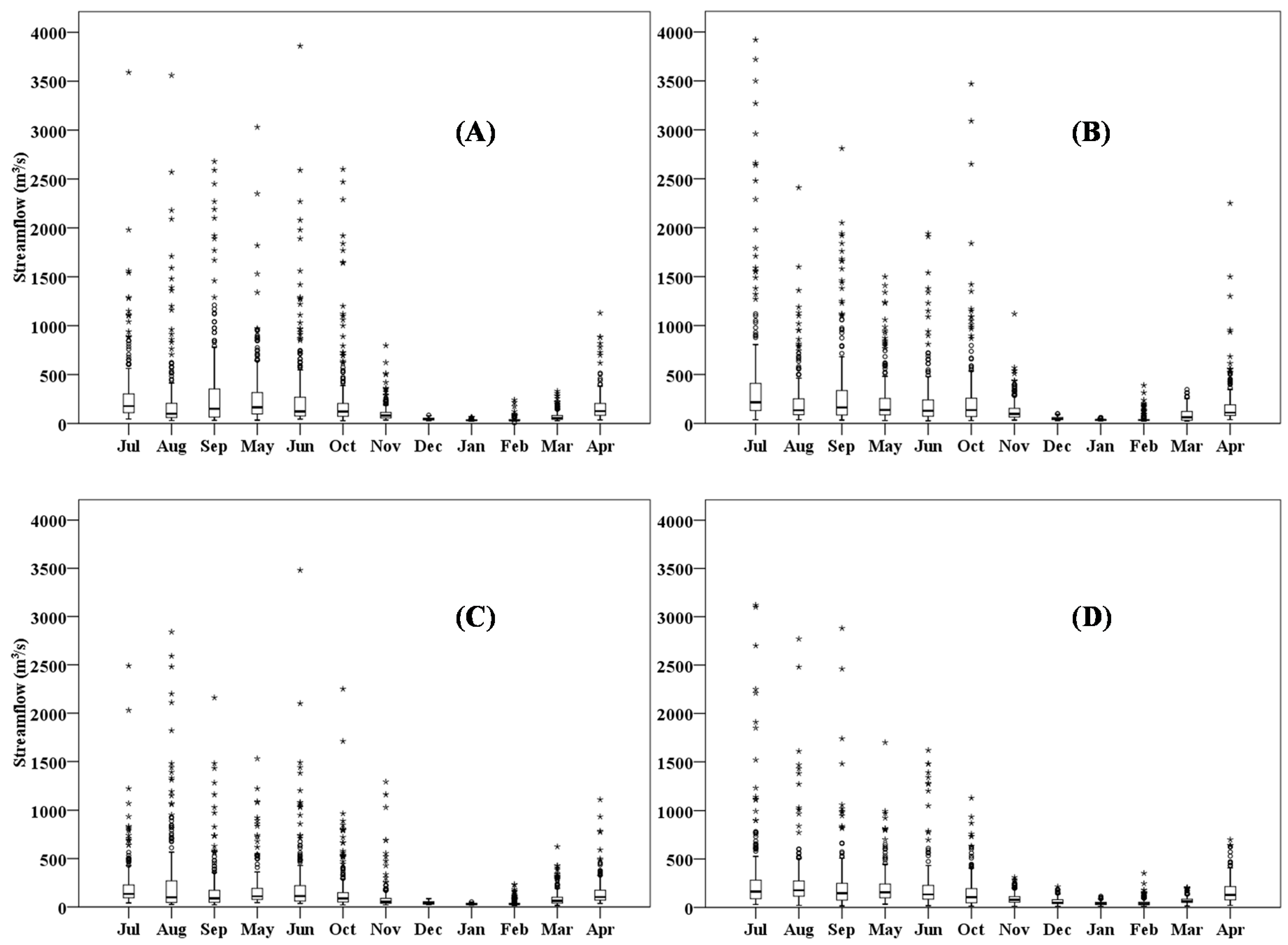
Figure 4 displays a box plot for the annual seasonal extreme streamflow data for each decade. The total annual number of days with extreme streamflow for the entire watershed for the 1970s, 1980s, 1990s, and 2000s were 306, 321, 291, and 196, respectively. The peak in the 1980s was well defined due to the frequency of the hydrometeorological days, which represented approximately 28.8% of all the data, while the low value in the 2000s represented approximately 17.6% of all the data.
The Wald–Wolfowitz test results (Z = −1.054, p-value = 0.387) of the streamflow at the Dongzhuang station showed that the data were independent at p < 0.05. The Mann–Kendall test results (K = −2.256, p-value = 0.021) showed that the yearly maximum streamflow increased significantly after 1999 at p < 0.05. The corresponding parameters were estimated by the ML methods. The results of the goodness-of-fit tests for selecting an appropriate probability distribution for the sub-watershed streamflow frequency analysis using the AIC and BIC criteria are summarized in Table 3. Out of 66 cases (two model selection criteria × 33 sub-watersheds), the LN2 distribution model was preferred for 53 cases (i.e., 80.3%), whereas the GEV distribution model was favored in the remaining 13 cases (i.e., 19.7%). Both model selection criteria favored the LN2 distribution over the GEV distribution, as shown in Table 3. These results demonstrated that the LN2 distribution was preferable to the GEV distribution for modeling the partial time series data for the selected watersheds. The empirical probability curves as well as the confidence intervals of the LN2 distribution for the observed streamflow at the watershed scale are presented in Figure 5.
3.3. Nonstationary Regional Frequency Analysis
By fitting the LN2 distribution with the ML parameter estimation method to the sub-watershed streamflow data, the maximum streamflow quantiles at each sub-watershed were estimated for average recurrence intervals (ARIs) of two, five, 10, 20, 100, and 1000 years to analyze the flood events in each sub-watershed.
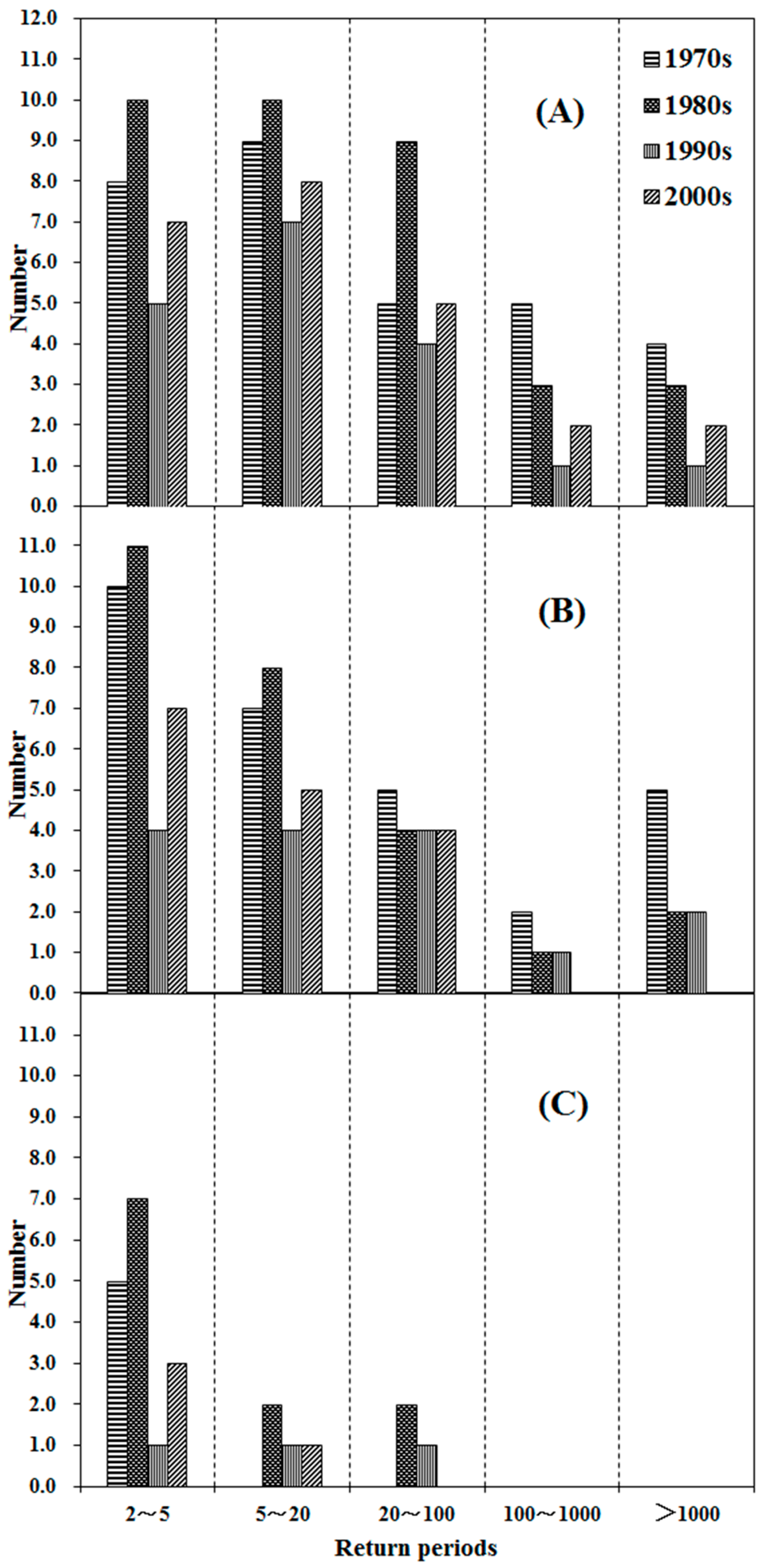
To analyze the seasonal variation in flood events at the watershed scale during different decades, the annual average number of flood events in different decades (1970s, 1980s, 1990s, and 2000s) were computed under different return levels (2–5, 5–20, 20–100, 100–1000, and >1000 years). The results are shown in Figure 6. The number of flood events during flood seasons for return periods covering two to 100 years, wet seasons for return periods covering two to 20 years, and dry seasons for the return periods of two to five years shows similar fluctuations. Similar variations can also be found for return periods that exceed 100, 20, and five years in flood seasons, wet seasons, and dry seasons, respectively. Compared with the lower and higher return periods, a significantly different flood event distribution is identified. As the seasons change (i.e., from the flood to dry season), the total number of flood events in each return periods change and the maximum and minimum numbers diminish and shift to shorter return periods.
For the return periods from two to five years, the flood events were most frequent during the 1980s in all seasons, and the flood events were least frequent in the 1990s for each season. For the return periods of five to 20 years, the maximum values occurred in the 1980s, whereas the minimum values occurred in the 1990s for both the flood and wet seasons. For the return periods of 20 to 100 years, the maximum values occurred in the 1980s for both the flood and dry seasons and in the 1970s for the wet season, and the minimum values were recorded in the 1990s for the flood season. The lowest values occurred in the 1980s, 1990s, and 2000s for the wet season, and the total number for the three decades was four. For the return periods of 100–1000 and >1000 years, the maximum values occurred in the 1970s for both the flood and wet seasons, whereas the minimum values were recorded in the 1990s for the flood season. Compared with the baseline return periods of two to five years, in the flood season, the mean annual number of flood events for the four decades increased for the return periods of five to 20 years and then showed a decreasing gradient for larger return periods. Similar variations occurred in each decade. In the wet season, compared with the baseline, the mean annual number of flood events over the four decades indicated a decreasing trend for return periods below 1000 years. Each decade exhibited similar dynamics. In the dry season, a strong gradient existed in the total number of events over the four decades.
Among the four decades, in the flood season, the highest number of events was found for the return periods of five to 20 years, and the lowest number was found for the return periods of >1000 years. The highest numbers were found for the return periods of two to five years in both the wet and dry seasons, while the lowest numbers were found for the return periods of 100 to 1000 years and the return periods of 20 to 100 years in the wet and dry seasons, respectively. Among the three seasons, the flood events in the flood season were more severe than in the other two seasons.
3.4. Contribution of Rainfall and Land Use to Flood Events
The performance of the PLS regression models is shown in Table 4. For the flood season, in the return periods of two to five years, the first component was dominated by forest on the negative side and explained 74.3% of the variation in flood events. The addition of the second component was dominated by rainfall, urban land, and farmland on the positive side and made the explanation approached 81.2% of the variation and generated the minimum mean square error of cross-validation (RMSECV) value. The addition of more components to the PLS regression models did not substantially improve the explanatory power but resulted in a higher RMSECV, indicating that the subsequent components were not strongly correlated with the residuals of the predicted variable according to [26]. For return periods of five to 20 years model, the first component was dominated by forest on the negative side, which explained 71.8% of the flood events variance in the dataset. The addition of the second component, dominated by rainfall, farmland, and urban land on the positive side, increased the model–explained variance to 78.0%. For the return periods of 20 to 100 and 100–1000 years, the first component was dominated by forest on the negative side, and the second component was dominated by urban land on the positive side. For the wet season, in return periods of two to five and five to 20 years, the first component was dominated by forest on the negative side, and the second component was dominated by rainfall, urban land, and farmland on the positive side. For the dry season, in the return periods of two to five years, the first component was dominated by forest on the negative side and farmland on the positive side, and the second component was dominated by rainfall and urban land on the positive side. In return periods > 5 years, the rainfall became to the dominate factor.
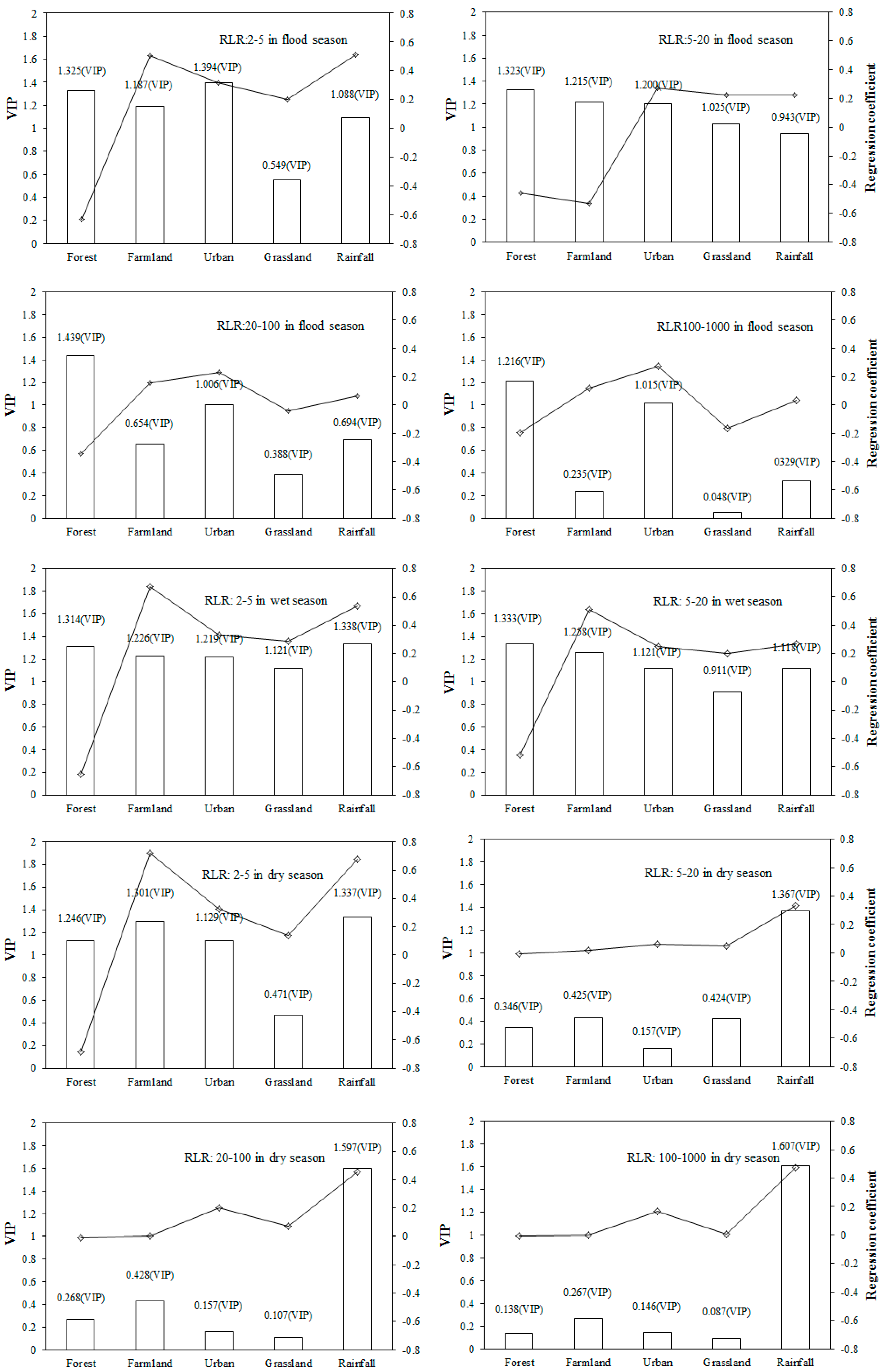
The relationship between the number of seasonal flood events (in the 1980s) and the proportion of land use types (1980s) was analyzed at the sub-watershed scale. Figure 7 shows the relative contributions of impact factors under different return periods. The influence of land use types on flood events decreased with increasing return periods. Farmland and urban areas had a positive effect on the number of events, while forest land had a negative effect. No statistically significant relationships were detected between grassland and flood events. For the flood and wet season, in the return periods of 2–5 and 5–20 years, the forest area had a significant negative effect on the number of flood events, while significant positive correlations were detected between both farmland and urban areas and flood events. VIP values of forest, farmland, and urban land (VIP > 1) were higher than those of grassland and rainfall. For the flood season, in the return periods of 20 to 100 and 100–1000 years, forest and urban land had VIP scores greater than 1, and rainfall, farmland, and grassland had VIP value less than 1, as shown in Figure 7. In the wet seasons, no statistically significant relationships between land use types and flood events were detected when the return period exceeded 100 years. For the dry season, in the return periods of two to five years, rainfall had the highest VIP score (1.337) and a larger positive regression (0.679), followed by the farmland (coefficient = 0.723; VIP = 1.301), forest (coefficient = −0.685; VIP = 1.246), and urban land (coefficient = 0.324; VIP = 1.129). These results show a significant negative correlation between the forest area and the number of flood events. Rainfall, farmland, and urban area had remarkable positive effects on the number of flood events. The VIP value (greater than 1) of rainfall was highest in return periods > 5 years in the dry season, followed by farmland, forest, urban land, and grassland with VIP values less than 1 (ranging from 0.428 to 0.087).
4. Discussion
The ability of the SWAT model to simulate the daily streamflow data in the frequency analysis has been demonstrated by many papers [21,23,40]. A high goodness-of-fit value for the monthly and daily streamflow suggests good model performance in our study. Table 2 shows good modeling results for the monthly streamflow, with a maximum Nash–Sutcliffe efficiency (ENS) of 0.80. In our study, daily streamflow ENS is less satisfactory than that of monthly streamflow, which is similar to other SWAT modeling studies [41,42]. For hydrologic evaluations performed at a monthly time interval, the model results are satisfactory when ENS values exceed 0.5. However, appropriate relaxing of the standard may be performed for daily time–step evaluations [32]. Thus, a daily ENS of 0.5 corresponds to a monthly ENS of approximately >0.8, as suggested by [43]. Therefore, the performance measures for the simulations range from satisfactory to good in all studied sub-watersheds according to [32]. This evaluation methodology is suggested by many studies [8,41,43,44]. Previously, we studied the Upper Du River watershed, which is a forest watershed similar to the Upper Honganjian watershed in China, using the same method and the results confirmed the satisfactory performance of SWAT [22,43,44]. The results of this study are consistent with Liu [45], which was a study of a runoff simulation in the Upper Honganjian watershed.
We address the relative importance of precipitation and land use types for flood events in 33 sub-watersheds. The most convenient and comprehensive description of the relative importance of predictors can be derived from exploring their VIP values [26]. For different return periods in each season, relevant fluctuations in the total number of events in each decade are found. These fluctuations are consistent with the variations in flood events in the Upper Honganjian watershed, implying that a similar pattern of the flood events seasonal distribution exists in specific return periods. However, there are significantly different dynamics for return periods that exceed 100 years in the flood season, return periods that exceed 20 years in the wet season, and return periods that exceed five years in the dry season. These results may be related to the coupling of precipitation, land use types, and anthropogenic construction [5,46].
The results in Figure 7 show that precipitation changes will influence flood events, especially at a two- to five-year return period in the flood and wet seasons. Precipitation could trigger a higher risk of floods in a watershed, and many complex factors (temperature, reservoirs, and drainage system) may also influence the streamflow volume [47]. Similar conclusions were reported by Zhang et al. [5], who showed that precipitation is one of the pivotal factors triggering hydrological alterations of flood events. The flood dynamics at return periods > 5 years may be attributed to the hydrological regulations of water reservoirs. Anthropogenic construction and management, such as dams and reservoirs, river training, and human water use affect the seasonality of flood events in these periods [48,49]. Reservoirs, dams, irrigation flow diversions, and flood control structures have been developed and generate significant hydrogeomorphic alterations with impacts occurring in both streams and catchments of the watershed [50]. Reservoirs and dams result in increased evapotranspiration (ET) and lead to fewer flood events, while seasonal withdrawals affect the seasonality of flood events [48]. Small reservoirs may lose up to 50% of their stored volume due to evaporation in many regions due to the high ratio of surface/volume area. Evaporation constitutes a major component of the water balance in the reservoirs and may significantly decrease flood events [51]. Moreover, in order to sustain and maintain the ecological integrity of watershed, numerous watershed management measures, such as management of flood utilization, establishing and maintaining minimum flow releases, or permitting controlled “flushing” releases that establish the necessary high flows for sediment transport have been applied. These hydrogeomorphic and watershed management practice impacts have profoundly influenced flood evolution and frequency [50]. In the dry season, the correlations between flood events and the precipitation amount shift from low to high values as the return period increases. This anomaly can be interpreted as follows: for a longer return period, the flood frequency depends on the initial soil moisture conditions [21]; therefore, the precipitation amount in the dry season determines the initial soil moisture conditions and indirectly influences the flood events that occur in the wet and flood seasons.
For each season, the influence of land use on flood events decreases with an increasing return period. Water management facilities have led to variations in hydrological events for a longer return period [4]. Our results reveal a strong influence of land use types on flood events for specific return periods; the number of flood events is also highly influenced by land use type, namely, forest, urban, and farmland areas. Farmland and urban areas are found to increase the number of flood events, while forest land results in fewer flood events. Similar results were reported by [47,52]. Farmland reduces evapotranspiration, enhances infiltration, increases the initial moisture stored in the soil, eventually increases the number of flood events [21]. The increased number of flood events associated with the expansion of urban areas can be explained as follows. With urbanization, infiltration is reduced by soil compaction and impervious surface additions, and water flushes more quickly through the watershed as a result of decreases in the hydraulic resistance of land surfaces and channels [53]. However, forest land increases evapotranspiration and tends to decrease the number of flood events [21]. For return periods of two to five years, the number of flood events is most closely related to the land use types of forest, urban, and farmland in the dry season, followed by the wet and flood seasons. This conclusion was also drawn by Liu et al. [54], who indicated that the impact of deforestation or reforestation on hydrological events is more significant in the dry season than in other seasons. In dry season, the effects of rainfall are greater than those of land use type. This phenomenon can be explained as follows. The dry season is not a growth period for most vegetation, and ET of forest and other land use types associated with flood events can be ignored [22]. In addition, compared with flood and wet seasons, interception of the forest canopy and undergrowth vegetation associated with throughfall in the dry season is generally lower, which mitigates the negative influences of forests on flood [53].
5. Conclusions
The SWAT model was used to estimate the daily streamflow for ungauged sub-watersheds. Exploratory data analysis and outlier detection were performed using box plots. Based on the maximum likelihood (ML) estimation method, Akaike information criterion (AIC), and Bayesian information criterion (BIC), the lognormal (LN2) distribution was preferable to the generalized extreme value (GEV) distribution to fit the partial time series streamflow data.
In low return periods, similar patterns existed for the flood event distribution. Significantly different patterns existed for return periods that exceeded 100 years in the flood season, return periods that exceeded 20 years in the wet season, and return periods that exceeded five years in the dry season. Rainfall and forest are pivotal factors triggering flood event alterations in lower return periods, and the flood events in higher return periods are attributed to the hydrological regulations of water management facilities. Farmland and urban areas were related to fewer flood events, while the presence of forest land was found to decrease the number of flood events. In the dry season, the influence of rainfall on flood events is much greater than that of land use.
The approach used in this study can help to easily select the optimal distributions for watersheds using ungauged sub-watersheds. The return periods and flood events can be simulated more precisely using optimal distributions. Moreover, flood-prone regions can be identified, which can provide a scientific foundation to determine flood-resistant measures by comparing the increased flood risk at different return levels.
Author Contributions
X.H. and P.H. conceived and designed the experiments; X.H. and L.W. performed the experiments; W.W. and P.H. analyzed the data; X.H. wrote the paper.
Funding
Financial support for this research was provided by the Project of Hydraulic Science and Technology of Jiang Xi province, China (KT201615); National Natural Science Foundation of China (No: 51509088); Henan province university scientific and technological innovation team (18IRTSTHN009); the Key Scientific Research Projects of Higher Education Institutions (18A170010); Henan Key Laboratory of Water Environment Simulation and Treatment (2017016).
Acknowledgments
We are truly grateful to editors and the anonymous reviewers for providing critical comments and thoughtful suggestions.
Conflicts of Interest
The authors declare no conflict of interest.
Appendix A
Appendix A.1. Grubbs and Beck (1972) Statistical Test
The observations are arranged in ascending order: x1 ≤ x2 ≤ … ≤ xn. Therefore, to test whether the largest observation, xn, in normal samples is too large, we compute
and
and refer the result to the table of Grubbs test [31], which provides various upper probability levels for Tn. A significance test of the smallest observation for normal samples is obtained by computing
To test the significance of the two largest observations, xn−1 and xn we compute
in which
in which
Appendix A.2. Wald–Wolfowitz Test
This test is used to compare two unmatched, supposedly continuous distributions, and the null hypothesis is that the two samples are distributed identically [55]. A run is a set of sequential values that are either all above or below the mean. To simplify computations, the data are first centered around their mean. To carry out the test, the total number of runs is computed along with the number of positive and negative values. A positive run is a sequence of values greater than zero, and a negative run is a sequence of values less than zero. We can then test whether the numbers of positive and negative runs are distributed equally in time. The test statistic is asymptotically normally distributed, and therefore, this test computes Z, the large sample test statistic, as follows:
in which R is the number of runs.
The null and alternative hypotheses are as follows:
When the large sample approach is in question, the test statistic calculated by the average of this formula will be compared with the values obtained from the standard normal table for the previously determined level of significance [55]. If the Z value is lower than or equal to the table value, then the H0 hypothesis must be rejected at the significance level of α.
Appendix A.3. Mann–Kendall Test
The Mann–Kendall (MK) statistic, S, is defined as follows:
where Xj represents the sequential data values, n is the length of the dataset, and
The statistic S is approximately normally distributed when n ≥ 8, with the mean and the variance as follows:
where ti is the number of ties of extent i.
The standardized test statistic (Z) of the MK test and the corresponding p-value (p) for the one–tailed test are given by
Appendix A.4. GEV Distributions
The distributions of extreme values (EV) were developed by Fisher and Tippett [58]. Families (Gumbel, Fréchet, and Weibull) of traditional EV were combined into the generalized extreme values (GEV) distribution with a cumulative distribution function by Jenkinson [59]:
where when k < 0 (Fre’chet), when k = 0 (Gumbel) and when k > 0 (Weibull). , a (>0), and are the location, the scale and the shape parameters, respectively.
Appendix A.5. LN2
In probability theory, a log-normal distribution (LN) is a continuous probability distribution of a random variable the logarithm of which is normally distributed. The probability density function of the two–parameter log–normal distribution (LN2) is:
in which , .
References
- Eagleson, P.S. Dynamics of flood frequency. Water Resour. Res. 1972, 8, 878–898. [Google Scholar] [CrossRef]
- Zaman, M.A.; Rahman, A.; Haddad, K. Regional flood frequency analysis in arid regions: A case study for Australia. J. Hydrol. 2012, 475, 74–83. [Google Scholar] [CrossRef]
- O’Brien, N.L.; Burn, D.H. A nonstationary index-flood technique for estimating extreme quantiles for annual maximum streamflow. J. Hydrol. 2014, 519, 2040–2048. [Google Scholar] [CrossRef]
- Haberlandt, U.; Radtke, I. Hydrological model calibration for derived flood frequency analysis using stochastic rainfall and probability distributions of peak flows. Hydrol. Earth Syst. Sci. 2014, 18, 353–365. [Google Scholar] [CrossRef] [Green Version]
- Zhang, Q.; Gu, X.; Singh, V.P.; Xiao, M. Flood frequency analysis with consideration of hydrological alterations: Changing properties, causes and implications. J. Hydrol. 2014, 519, 803–813. [Google Scholar] [CrossRef]
- Rao, A.R.; Hamed, K.H. Flood Frequency Analysis; CRC Press: New York, NY, USA, 2000; p. 355. [Google Scholar]
- Wei, W.; Chen, L.D.; Fu, B.J.; Huang, Z.L.; Wu, D.P.; Gui, L.D. The effect of land uses and rainfall regimes on runoff and soil erosion in the semi-arid loess hilly area. China. J. Hydrol. 2007, 335, 247–258. [Google Scholar] [CrossRef]
- Yan, B.; Fang, N.F.; Zhang, P.C.; Shi, Z.H. Impacts of land use change on watershed streamflow and sediment yield: An assessment using hydrologic modelling and partial least squares regression. J. Hydrol. 2013, 484, 26–37. [Google Scholar] [CrossRef]
- Karim, F.; Hasan, M.; Marvanek, S. Evaluating annual maximum and partial duration series for estimating frequency of small magnitude floods. Water 2017, 9, 481. [Google Scholar] [CrossRef]
- Benkhaled, A.; Higgins, H.; Chebana, F.; Necir, A. Frequency analysis of annual maximum suspended sediment concentrations in Abiod wadi, Biskra (Algeria). Hydrol. Process. 2014, 28, 3841–3854. [Google Scholar] [CrossRef]
- Khaliq, M.N.; Ouarda, T.B.M.J.; Ondo, J.C.; Gachon, P.; Bobée, B. Frequency analysis of a sequence of dependent and/or non-stationary hydro-meteorological observations: A review. J. Hydrol. 2006, 329, 534–552. [Google Scholar] [CrossRef]
- Schendel, T.; Thongwichian, R. Considering historical flood events in flood frequency analysis: Is it worth the effort? Adv. Water Resour. 2017, 105, 144–153. [Google Scholar] [CrossRef]
- Obeysekera, J.; Salas, J.D. Quantifying the uncertainty of design floods under nonstationary conditions. J. Hydrol. Eng. 2013, 19, 1438–1446. [Google Scholar] [CrossRef]
- She, D.X.; Xia, J.; Zhang, D.; Ye, A.Z.; Sood, A. Regional extreme-dry-spell frequency analysis using the L-moments method in the middle reaches of the Yellow River Basin, China. Hydrol. Process. 2014, 28, 4694–4707. [Google Scholar] [CrossRef]
- Tramblay, Y.; St–Hilaire, A.; Ouarda, T.B.M.J. Frequency analysis of maximum annual suspended sediment concentrations in North America. Hydrol. Sci. J. 2008, 53, 236–252. [Google Scholar] [CrossRef]
- Milly, P.C.D.; Julio, B.; Malin, F.; Robert, M.H.; Zbigniew, W.K.; Dennis, P.L.; Ronald, J.S. Stationarity is dead: Whither water management. Science 2008, 319, 573–574. [Google Scholar] [CrossRef] [PubMed]
- Zhang, X.; Harvey, K.D.; Hogg, W.D.; Yuzuk, T.R. Trends in Canadian streamflow. Water Resour. Res. 2001, 37, 987–999. [Google Scholar] [CrossRef]
- Leclerc, M.; Ouarda, T.B. Non-stationary regional flood frequency analysis at ungauged sites. J. Hydrol. 2007, 343, 254–265. [Google Scholar] [CrossRef]
- Kovalets, I.V.; Kivva, S.L.; Udovenko, O.I. Usage of the WRF/DHSVM model chain for simulation of extreme floods in mountainous areas: A pilot study for the Uzh River Basin in the Ukrainian Carpathians. Nat. Hazards 2014, 75, 2049–2063. [Google Scholar] [CrossRef]
- Behera, S.; Panda, R.K. Evaluation of management alternatives for an agricultural watershed in a sub-humid subtropical region using a physical process based model. Agric. Ecosyst. Environ. 2006, 113, 62–72. [Google Scholar] [CrossRef]
- Ryu, J.H.; Lee, J.H.; Jeong, S.; Park, S.K.; Han, K. The impacts of climate change on local hydrology and low flow frequency in the Geum River Basin, Korea. Hydrol. Process. 2011, 25, 3437–3447. [Google Scholar] [CrossRef]
- Huang, X.D.; Shi, Z.H.; Fang, N.F.; Li, X. Influences of land use change on baseflow in mountainous watersheds. Forests 2016, 7, 16. [Google Scholar] [CrossRef]
- Dessu, S.B.; Melesse, A.M. Modelling the rainfall-runoff process of the Mara River basin using the Soil and Water Assessment Tool. Hydrol. Process. 2012, 26, 4038–4049. [Google Scholar] [CrossRef]
- Artita, K.S.; Kaini, P.; Nicklow, J.W. Examining the possibilities: Generating alternative watershed-scale BMP designs with evolutionary algorithms. Water Resour. Manag. 2013, 27, 3849–3863. [Google Scholar] [CrossRef]
- Zhou, F.; Xu, Y.; Chen, Y.; Xu, C.Y.; Gao, Y.; Du, J. Hydrological response to urbanization at different spatio-temporal scales simulated by coupling of CLUE-S and the SWAT model in the Yangtze River Delta region. J. Hydrol. 2013, 485, 113–125. [Google Scholar] [CrossRef]
- Abdi, H.; Williams, L.J. Principal component analysis. Wiley Interdiscip. Rev. Comput. Stat. 2010, 2, 433–459. [Google Scholar] [CrossRef] [Green Version]
- Buondonno, A.; Amenta, P.; Viscarra-Rossel, R.A.; Leone, A.P. Prediction of soil properties with plsr and vis-nir spectroscopy: Application to mediterranean soils from southern Italy. Curr. Anal. Chem. 2012, 8, 283–299. [Google Scholar]
- Geladi, P.; Sethson, B.; Nyström, J.; Lillhonga, T.; Lestander, T.; Burger, J. Chemometrics in spectroscopy. Spectrochim. Acta B At. Spectrosc. 2004, 59, 1347–1357. [Google Scholar] [CrossRef]
- Li, S.; Li, J.; Zhang, Q. Water quality assessment in the rivers along the water conveyance system of the Middle Route of the South to North Water Transfer Project (China) using multivariate statistical techniques and receptor modeling. J. Hazard. Mater. 2011, 195, 306–317. [Google Scholar] [CrossRef] [PubMed]
- Soil Survey Staff. Soil Taxonomy, A Basic System of Soil Classification for Making and Interpreting Soil Surveys, 2nd ed.; Agriculture Handbook No. 436; USDA Natural Resources Conservation Service, U.S. Government Printing 23 Office: Washington, DC, USA, 1999; pp. 160–162, 494–495.
- Duan, Q.D.; Gupta, V.K.; Sorooshian, S. Effective and efficient global optimization for conceptual rainfall-runoff models. Water Resour. Res. 1992, 28, 1015–1031. [Google Scholar] [CrossRef]
- Moriasi, D.N.; Arnold, J.G.; Van Liew, M.W.; Bingner, R.L.; Harmel, R.D.; Veith, T.L. Model evaluation guidelines for systematic quantification of accuracy in watershed simulations. Trans. ASABE 2007, 50, 885–900. [Google Scholar] [CrossRef]
- Grubbs, F.E.; Beck, G. Extension of sample sizes and percentage points for significance tests of outlying observations. Technometrics 1972, 14, 847–854. [Google Scholar] [CrossRef]
- Cunderlik, J.M.; Ouarda, T.B. Regional flood–duration–frequency modeling in the changing environment. J. Hydrol. 2006, 318, 276–291. [Google Scholar] [CrossRef]
- Akaike, H. A new look at the statistical model identification. IEEE Trans. Automat. Cont. 1974, 19, 716–723. [Google Scholar] [CrossRef]
- Schwarz, G. Estimating the dimension of a model. Ann. Stat. 1978, 6, 461–464. [Google Scholar] [CrossRef]
- Calenda, G.; Mancini, C.P.; Volpi, E. Selection of the probabilistic model of extreme floods: The case of the River Tiber in Rome. J. Hydrol. 2009, 371, 1–11. [Google Scholar] [CrossRef]
- Laio, F.; Di Baldassarre, G.; Montanari, A. Model selection techniques for the frequency analysis of hydrological extremes. Water Resour. Res. 2009, 45, W07416. [Google Scholar] [CrossRef]
- Sahu, N.; Behera, S.K.; Yamashiki, Y.; Takara, K.; Yamagata, T. IOD and ENSO impacts on the extreme stream-flows of Citarum river in Indonesia. Clim. Dynam. 2012, 39, 1673–1680. [Google Scholar] [CrossRef]
- Wang, G.Q.; Yang, H.; Wang, L.; Xu, Z.; Xue, B. Using the SWAT model to assess impacts of land use changes on runoff generation in headwaters. Hydrol. Process. 2014, 28, 1032–1042. [Google Scholar] [CrossRef]
- Seidou, O.; Ramsay, A.; Nistor, I. Climate change impacts on extreme floods I: Combining imperfect deterministic simulations and non-stationary frequency analysis. Nat. Hazards 2011, 61, 647–659. [Google Scholar] [CrossRef]
- Fu, C.; James, A.L.; Yao, H. SWAT-CS: Revision and testing of SWAT for Canadian Shield catchments. J. Hydrol. 2014, 511, 719–735. [Google Scholar] [CrossRef]
- Shi, Z.H.; Huang, X.D.; Ai, L.; Fang, N.F.; Wu, G.L. Quantitative analysis of factors controlling sediment yield in mountainous watersheds. Geomorphology 2014, 226, 193–201. [Google Scholar] [CrossRef]
- Shi, Z.H.; Ai, L.; Li, X.; Huang, X.D.; Wu, G.L.; Liao, W. Partial least-squares regression for linking land-cover patterns to soil erosion and sediment yield in watersheds. J. Hydrol. 2013, 498, 165–176. [Google Scholar] [CrossRef]
- Liu, H.M. The Runoff Simulation of SWAT Model Coupled with the ECMWF Dataset. Master Thesis, North China University of Water Resources and Electric Power, Zhengzhou, China, 2017. [Google Scholar]
- Koutroulis, A.G.; Tsanis, I.K.; Daliakopoulos, I.N. Seasonality of floods and their hydrometeorologic characteristics in the island of Crete. J. Hydrol. 2010, 394, 90–100. [Google Scholar] [CrossRef]
- Condon, L.E.; Gangopadhyay, S.; Pruitt, T. Climate change and non–stationary flood risk for the upper Truckee River basin. Hydrol. Earth Syst. Sci. 2015, 19, 159–175. [Google Scholar] [CrossRef]
- Döll, P. Vulnerability to the impact of climate change on renewable groundwater resources: A global-scale assessment. Environ. Res. Lett. 2009, 4, 035006. [Google Scholar] [CrossRef]
- Villarini, G.; Smith, J.A.; Serinaldi, F.; Ntelekos, A.A. Analyses of seasonal and annual maximum daily discharge records for central Europe. J. Hydrol. 2011, 399, 299–312. [Google Scholar] [CrossRef]
- Magilligan, F.J.; Nislow, K.H. Long-term changes in regional hydrologic regime following impoundment in a humid-climate watershed. J. Am. Water Resour. As. 2001, 37, 1551–1569. [Google Scholar] [CrossRef]
- Ashraf, M.; Kahlown, M.A.; Ashfaq, A. Impact of small dams on agriculture and groundwater development: A case study from Pakistan. Agric. Water Manag. 2007, 92, 90–98. [Google Scholar] [CrossRef]
- Baratti, E.; Montanari, A.; Castellarin, A.; Salinas, J.L.; Viglione, A.; Bezzi, A. Estimating the flood frequency distribution at seasonal and annual time scales. Hydrol. Earth Syst. Sci. 2012, 16, 4651–4660. [Google Scholar] [CrossRef] [Green Version]
- Price, K. Effects of watershed topography, soils, land use, and climate on baseflow hydrology in humid regions: A review. Prog. Phys. Geogr. 2011, 35, 465–492. [Google Scholar] [CrossRef]
- Liu, Y.Y.; Zhang, X.N.; Xia, D.Z.; You, J.S.; Rong, Y.S.; Bakir, M. Impacts of land–use and climate changes on hydrologic processes in the Qingyi River watershed, China. J. Hydrol. Eng. 2013, 18, 1495–1512. [Google Scholar] [CrossRef]
- Daniel, W.W. Applied Nonparametric Statistics, 2nd ed.; PWS-Kent: Boston, MA, USA, 1990. [Google Scholar]
- Mann, H.B. Nonparametric tests against trend. Econometrica 1945, 13, 245–259. [Google Scholar] [CrossRef]
- Kendall, M.G. Rank Correlation Methods; Oxford Univ. Press: New York, NY, USA, 1975. [Google Scholar]
- Fisher, R.A.; Tippett, L.H.C. Limiting forms of the frequency distribution of the largest or the smallest member of a sample. Math. Proc. Camb. 1928, 24, 180–190. [Google Scholar] [CrossRef]
- Jenkinson, A.F. The frequency distributions of the annual maximum (or minimum) values of meteorological elements. Q. J. R. Meteorol. Soc. 1955, 81, 145–158. [Google Scholar] [CrossRef]
Figure 1.
Location of Upper Honganjian watershed with observation stations.

Figure 2.
Land uses (farmland, urban, forest, and grassland) map for the 1980s in the Upper Honganjian watershed.
Figure 2.
Land uses (farmland, urban, forest, and grassland) map for the 1980s in the Upper Honganjian watershed.

Figure 3.
Map showing the sub-watersheds in the Upper Honganjian watershed.

Figure 4.
Box plot for the monthly extreme streamflow data in the flood season (July, August, and September), wet season (May, June, and October), and dry season (November–April) in the 1970s (A), 1980s (B), 1990s (C), and 2000s (D).
Figure 4.
Box plot for the monthly extreme streamflow data in the flood season (July, August, and September), wet season (May, June, and October), and dry season (November–April) in the 1970s (A), 1980s (B), 1990s (C), and 2000s (D).

Figure 5.
Empirical probability curves and confidence intervals (Conf. Int.) of the LN2 distributions for the observed stream flows at the watershed scale. The scale of y-axis is normal probability.
Figure 5.
Empirical probability curves and confidence intervals (Conf. Int.) of the LN2 distributions for the observed stream flows at the watershed scale. The scale of y-axis is normal probability.

Figure 6.
The average annual number of flood events under different return periods, i.e., 2 to 5, 5 to 20, 20 to 100, 100 to 1000, and >1000 years, for various decades (1970s, 1980s, 1990s, and 2000s) in the flood season (A), wet season (B), and dry season (C).
Figure 6.
The average annual number of flood events under different return periods, i.e., 2 to 5, 5 to 20, 20 to 100, 100 to 1000, and >1000 years, for various decades (1970s, 1980s, 1990s, and 2000s) in the flood season (A), wet season (B), and dry season (C).

Figure 7.
Regression coefficients (lines) and the variable influence on projection (VIP) (bars) of each factor.
Figure 7.
Regression coefficients (lines) and the variable influence on projection (VIP) (bars) of each factor.


Table 1.
Parameters for streamflow calibration of the SWAT in the Upper Honganjian watershed.
| Parameter | Definition | Calibrated Value | |
|---|---|---|---|
| basin.bsn | ESCO | Soil evaporation compensation factor | 0.19 |
| basin.bsn | EPCO | Plant water uptake compensation factor | 1 |
| basin.bsn | SURLAG | Surface runoff lag time | 4 |
| .GW | GW_DELAY | Groundwater delay | 31 |
| .GW | GW_REVAP | Groundwater revap | 0.06 |
| .GW | ALPHA_BF | Baseflow alpha factor | 0.043 |
| .soil | SOL_AWC | Available water capacity of the soil layer | 0.2 |
| .sub | CH_N1 | Manning’s ‘n’ value for tributary channels | 0.014 |
| .rte | CH_N2 | Manning’s ‘n’ value for the main channel | 0.014 |
| .mgt | CN2 | SCS curve number | 62 (Forest) |
| 77 (Grassland) | |||
| 78 (Farmland) | |||
| 79 (Urban) |
Table 2.
Accuracy of the SWAT model calibration and validation in the Upper Honganjian watershed.
| Station | Period | ENSa | PBIASb | R2 |
|---|---|---|---|---|
| Monthly–Streamflow | Calibration (1972–1981) | 0.80 | –0.10 | 0.81 |
| Validation (1982–1991) | 0.77 | –0.09 | 0.87 | |
| Validation (1992–2001) | 0.75 | –0.13 | 0.80 | |
| Overall (1972–2001) | 0.77 | –0.11 | 0.83 | |
| Daily–Streamflow | Calibration (1971–1980) | 0.58 | –0.10 | 0.62 |
| Validation (1981–1990) | 0.56 | –0.09 | 0.67 | |
| Validation (1991–2000) | 0.52 | –0.11 | 0.62 | |
| Overall (1971–2000) | 0.55 | –0.10 | 0.64 |
aENS = Nash–Sutcliffe efficiency; b PBIAS = Percent Bias.
Table 3.
Summary of the goodness–of–fit tests for the 33 sub-watersheds.
| Distribution | AIC | BIC | ||
|---|---|---|---|---|
| LN2 a | GEV b | LN2 | GEV | |
| No. of sub-watersheds being selected | 26 | 7 | 27 | 6 |
| Percentage of sub-watersheds (%) | 78.8 | 21.2 | 81.8 | 18.2 |
a Sampling LN2 = lognormal; b Sampling GEV = generalized extreme value.
Table 4.
Summary of PLS regression for floods in each season.
| Response Y | R2 a | Component | Explained in Y (%) | Cumulative Explained in Y (%) | RMSECV b | |
|---|---|---|---|---|---|---|
| Seasons | Return Periods (Years) | |||||
| Flood | 2–5 | 0.81 | 1 | 74.3 | 74.3 | 0.89 |
| 2 | 6.9 | 81.2 | 0.80 | |||
| 3 | 0.1 | 81.3 | 0.81 | |||
| 5–20 | 0.79 | 1 | 71.8 | 71.8 | 4.17 | |
| 2 | 6.2 | 78.0 | 3.97 | |||
| 3 | 1.4 | 79.4 | 4.05 | |||
| 20–100 | 0.70 | 1 | 67.9 | 67.9 | 0.75 | |
| 2 | 2.4 | 70.3 | 0.73 | |||
| 3 | 0.1 | 70.4 | 0.74 | |||
| 100–1000 | 0.64 | 1 | 60.2 | 60.2 | 5.55 | |
| 2 | 3.1 | 63.3 | 5.28 | |||
| 3 | 0.8 | 64.1 | 5.47 | |||
| Wet | 2–5 | 0.82 | 1 | 75.1 | 75.1 | 0.71 |
| 2 | 5.6 | 80.7 | 0.64 | |||
| 3 | 1.3 | 82.0 | 0.61 | |||
| 4 | 0.4 | 82.4 | 0.65 | |||
| 5–20 | 0.79 | 1 | 71.3 | 71.3 | 0.85 | |
| 2 | 6.6 | 77.9 | 0.80 | |||
| 3 | 1.2 | 79.1 | 0.81 | |||
| Wet | 20–100 | 0.34 | 1 | 28.3 | 28.3 | 0.79 |
| 2 | 3.9 | 32.2 | 0.69 | |||
| 3 | 1.6 | 33.8 | 0.71 | |||
| 100–1000 | 0.27 | 1 | 22.2 | 22.2 | 0.65 | |
| 2 | 4.5 | 26.7 | 0.59 | |||
| 3 | 0.3 | 27.0 | 0.63 | |||
| Dry | 2–5 | 0.84 | 1 | 78.5 | 78.5 | 0.91 |
| 2 | 3.9 | 82.4 | 0.88 | |||
| 3 | 1.6 | 84.0 | 0.84 | |||
| 4 | 0.2 | 84.2 | 0.85 | |||
| 5–20 | 0.61 | 1 | 60.0 | 60.0 | 0.74 | |
| 2 | 0.9 | 60.9 | 0.68 | |||
| 3 | 0.1 | 61.0 | 0.69 | |||
| 20–100 | 0.69 | 1 | 67.2 | 67.2 | 0.65 | |
| 2 | 1.6 | 68.8 | 0.54 | |||
| 3 | 0.1 | 68.9 | 0.58 | |||
| 100–1000 | 0.76 | 1 | 74.2 | 74.2 | 0.54 | |
| 2 | 1.6 | 75.8 | 0.49 | |||
| 3 | 0.2 | 76.0 | 0.52 | |||
a Sampling R2 = goodness of fit; b RMSECV = cross-validated root mean squared error.
© 2018 by the authors. Licensee MDPI, Basel, Switzerland. This article is an open access article distributed under the terms and conditions of the Creative Commons Attribution (CC BY) license (http://creativecommons.org/licenses/by/4.0/).
Share and Cite
MDPI and ACS Style
Huang, X.-d.; Wang, L.; Han, P.-p.; Wang, W.-c. Spatial and Temporal Patterns in Nonstationary Flood Frequency across a Forest Watershed: Linkage with Rainfall and Land Use Types. Forests 2018, 9, 339. https://doi.org/10.3390/f9060339
AMA Style
Huang X-d, Wang L, Han P-p, Wang W-c. Spatial and Temporal Patterns in Nonstationary Flood Frequency across a Forest Watershed: Linkage with Rainfall and Land Use Types. Forests. 2018; 9(6):339. https://doi.org/10.3390/f9060339
Chicago/Turabian StyleHuang, Xu-dong, Ling Wang, Pei-pei Han, and Wen-chuan Wang. 2018. "Spatial and Temporal Patterns in Nonstationary Flood Frequency across a Forest Watershed: Linkage with Rainfall and Land Use Types" Forests 9, no. 6: 339. https://doi.org/10.3390/f9060339
Note that from the first issue of 2016, this journal uses article numbers instead of page numbers. See further details here.