A Generalized Lidar-Based Model for Predicting the Merchantable Volume of Balsam Fir of Sites Located along a Bioclimatic Gradient in Quebec, Canada

Abstract

Lidar-based models rely on an optimal relationship between the field and the lidar data for accurate predictions of forest attributes. This relationship may be altered by the variability in the stand growth conditions or by the temporal discrepancy between the field inventory and the lidar survey. In this study, we used lidar data to predict the timber merchantable volume (MV) of five sites located along a bioclimatic gradient of temperature and elevation. The temporal discrepancies were up to three years. We adjusted a random canopy height coefficient (accounting for the variability amongst sites), and a growth function (accounting for the growth during the temporal discrepancy), to the predictive model. The MV could be predicted with a pseudo-R² of 0.86 and a residual standard deviation of 24.3 m³ ha⁻¹. The average biases between the field-measured and the predicted MVs were small. The variability of MV predictions was related to the bioclimatic gradient. Fixed-effect models that included a bioclimatic variable provided similar prediction accuracies. This study suggests that the variability amongst sites, the occurrence of a bioclimatic gradient and temporal discrepancies are essential in building a generalized lidar-based model for timber volume.

1. Introduction

Forest stands often develop a diversity of canopy structures across space and time. The diversity may result from the natural dynamics in stands through time (e.g., growth, mortality, succession, stand composition), the variability of biophysical factors (e.g., soil, climate, elevation) or human activities [1,2]. Boucher et al. [1] for example, stated that disturbance regimes and climate have an effect on canopy structures. Laflèche et al. [3] showed that site characteristics, species composition, and climate influence site productivity.

Canopy structures can be described through forest attributes measured during field inventories (e.g., canopy cover, height, diameter, stand volume) or through remote sensing tools such as the light detection and ranging (lidar) [4]. Lidar is an active sensor which uses pulses of laser light to measure the distance to a target and record the strength of light backscattering from this target. It generates a point cloud which is a three-dimensional representation of the volumetric interaction between pulse photons and the target. It has been extensively used in forestry to describe the vertical structure of stands [5,6,7]. Metrics can be calculated from the point clouds to statistically describe them (e.g., height metrics, canopy cover metrics). They are often used as explanatory variables to model forest attributes such as basal area, timber merchantable volume, biomass, etc. [8,9,10,11].

Spatially extensive acquisitions of lidar datasets are now possible, making this tool attractive for large-scale inventories [12,13]. Such inventories often require several lidar surveys. Combining the resulting datasets is challenging, especially when there is variability amongst the sites distributed across a given survey area, or when time has elapsed between the field inventory and the lidar survey (temporal discrepancy). In this situation, it is difficult to transfer a site-specific model to another location and therein obtain the same prediction accuracy.

Recent research has ways to accurately predict forest attributes from lidar over large-scale areas. Hansen et al. [2] for example, included biophysical variables (climate, topography, and soil) in their model when predicting lidar canopy height and canopy cover for five ecoregions located along a 4000 km transect. Næsset and Gobakken [14] and Nilsson et al. [15] calibrated site-specific models to predict forest attributes from lidar and combined the models’ outputs to make predictions at a large-scale. Their approach allowed for accurate predictions locally but required several models for working at the large-scale level. and opted for a general mixed-effect model to predict timber volume, biomass or dominant height of multiple sites. Both authors obtained an overall goodness comparable to the site-specific (local) models. This approach offered the advantage of building a single predictive model which could be adapted to the specific conditions found in the different sites.

Several questions remain when predicting forest attributes of different sites in an operational context, including the following: (1) Does the combination of multiple lidar datasets in a generalized predictive model increase the bias at each site? (2) Does accounting for the variability in sites limit the model biases at each site? (3) How should forest attributes be predicted outside the range of the studied sites? and (4) Do temporal discrepancies between field and lidar acquisitions have an effect on the model prediction accuracy? This study, therefore, aims at analyzing the effects of variability amongst sites and temporal discrepancies on the prediction accuracy of timber merchantable volume of sites located along a bioclimatic gradient.

2. Materials and Methods

2.1. Study Sites

Various bioclimatic domains exist throughout the province of Quebec, Eastern Canada [16]. Five study sites populated by balsam fir (Abies balsamea (L.) Mill) were selected along a bioclimatic gradient of temperature, precipitation, elevation and growing degree days (calculated with a 5 °C reference temperature), Figure 1. The Mauricie_south and Mauricie_north sites are located in the Mauricie region in central Quebec (47.0° N, 73.0° W). The Mauricie_south covers an area of 4364 km². It is part of the sugar maple (Acer saccharum Marshall)/yellow birch (Betula alleghaniensis Britt.) domain. The Mauricie_north site covers an area of 4630 km². It is part of the balsam fir/yellow birch domain which is a transition zone between the temperate and the boreal forests. The Montmorency site is located in central Quebec (47.3° N, 71.1° W). It covers an area of 66 km². It is part of the balsam fir/white birch (Betula papyrifera Marshall) domain. Two other sites are located in the Saguenay-Lac-St-Jean (SLSJ) region in northern Quebec (49.7° N, 71.5° W). The SLSJ_south covers an area of 5937 km². It is part of the balsam fir/white birch and the black spruce (Picea mariana (Mill.) Britton, Sterns & Poggenburg)/moss (Bryophyta) domains. The SLSJ_north site covers an area of 6093 km². It is part of the black spruce/moss domain where balsam fir stands are preferentially located on the slope of hills.

The field and the lidar data were obtained from the Quebec provincial forest ministry - Ministère des Forêts, de la Faune et des Parcs (MFFP) and the Montmorency Research Forest [17,18,19]. The field data were acquired following a uniform inventory protocol while the lidar data were generated through surveys with variable acquisition parameters.

2.2. Field Plot Data

The field data were collected in circular plots (radius = 11.28 m, area = 400 m²). The plot center positions were georeferenced using a precision GPS + Glonass receiver. Field plots were selected following these criteria: (1) balsam fir was the dominant species (>50%); and (2) the dominant height was above 7 m. The resulting sample was comprised of 295 plots, with 40 plots inventoried at the Mauricie_south site (in 2012), 55 at the Mauricie_north (in 2012), 93 at the Montmorency forest (between 2009–2013), 74 at the SLSJ_south (in 2016), and 33 at the SLSJ_north (in 2016). Trees with a diameter at breast height (dbh) above 9 cm (merchantable trees) were measured using a diameter tape. Tree height was calculated using a height–diameter based-equation following Bégin and Raulier [20]:

$${\mathrm{H}}_{\mathrm{ij}}=1.3+\left[{\mathrm{DBH}}_{\mathrm{ij}}^2/{\left({\mathsf{\beta }}_{1\mathrm{j}}{+\mathsf{\beta }}_{2\mathrm{j}}\times {\mathrm{DBH}}_{\mathrm{ij}}\right)}^2\right]{+\mathsf{\epsilon }}_{\mathrm{ij}},\mathrm{with}{\mathsf{\beta }}_{1,2\mathrm{j}}={\mathsf{\beta }}_0{+\mathsf{\beta }}_{\mathrm{k}}\times {\mathrm{z}}_{\mathrm{k}}{+\mathsf{\delta }}_{\mathrm{j}}$$

(1)

where ${\mathrm{H}}_{\mathrm{ij}}$ is the total height of the ${\mathrm{i}}^{\mathrm{th}}$ tree of the ${\mathrm{j}}^{\mathrm{th}}$ plot, ${\mathrm{DBH}}_{\mathrm{ij}}$ the diameter at breast height, ${\mathsf{\beta }}_0{-\mathsf{\beta }}_{\mathrm{k}}$ the model parameters, ${\mathrm{z}}_{\mathrm{k}}$ the k explanatory variables, and ${\mathsf{\epsilon }}_{\mathrm{ij}}$ the error term and ${\mathsf{\delta }}_{\mathrm{j}}$ the plot random coefficients.

The height-diameter ratio (H–D ratio) of each plot was calculated by dividing the average plot height (weighted against the basal area) by the average plot dbh (weighted against the basal area). This ratio accounts for the tree morphology resulting from growth conditions [21]. The field merchantable volume (MV) defined as the volume under bark for stems greater than 9 cm diameter excluding the stump and tip, was calculated following Fortin et al. [22]. The climatic data (temperature, precipitation, growing degree days (gdds)) were derived from the MFFP forest inventory database using the BioSIM software [19].

Table 1. Summary of the field data ^a.

Field Characteristics	Study Sites
	Mauricie_South	Mauricie_North	Montmorency	SLSJ_South	SLSJ_North
Year of field inventory	2012	2012	2009–2013	2016	2016
Number of sample plots	40	63	100	78	40
Dominant height (m)	17.5 ± 2.0	19.0 ± 2.4	15.2 ± 4.3	17.5 ± 2.5	18.2 ± 2.6
Balsam fir height–diameter ratio	0.99 ± 0.1	0.98 ± 0.1	0.94 ± 0.1	0.96 ± 0.1	0.88 ± 0.1
Merchantable tree density (trees ha−1)	1448 ± 511	1176 ± 429	1486 ± 534	1360 ± 536	976 ± 243
Merchantable volume (m3 ha−1)	139.1 ± 48.0	170.9 ± 60.5	139.2 ± 89.9	137.1 ± 55.1	129.1 ± 44.5
Species composition	Balsam fir (85%), Birch (8%), Spruce (5%)	Balsam fir (81%), Birch (6%), Poplar (6%)	Balsam fir (82%), Spruce (10%), Birch (6%),	Balsam fir (78%), Spruce (20%), Birch (2%)	Balsam fir (72%), Spruce (17%), Birch (9%)
Mean annual temperature (°C)	2.3 ± 0.5	2.1 ± 0.4	−0.1 ± 0.5	0.4 ± 0.7	−1.2 ± 0.2
Annual precipitation (mm)	1015.3 ± 29.3	1041.9 ± 56.8	1430.1 ± 40.0	852.4 ± 32.6	916.4 ± 7.4
Elevation (m)	375.5 ± 73.7	367.3 ± 79.7	760.2 ± 95.0	385.6 ± 116.8	637.3 ± 51.2
Growing degree days (°C)	1407.5 ± 94.0	1385.3 ± 77.9	939.4 ± 73.0	1222.2 ± 94.9	1022.2 ± 41.1

^a average and standard deviation of the field characteristics.

provides a summary of the field data for the study sites.

2.3. Lidar Data and Variable Generation

The lidar surveys were conducted in leaf-on conditions in 2014 at the Mauricie_south and Mauricie_north sites, 2011 at the Montmorency site, 2013 at the SLSJ_south site, and 2013–2014 at the SLSJ_north site. They were supplied by various survey providers. Ground-classified returns were interpolated to construct a digital terrain model (dtm) using LAStools software (version 150526 unlicensed, rapidlasso GmbH, Gilching, Germany) [23]. The height of returns was normalized by measuring the elevation difference relative to the underlying terrain model. A 2 m threshold was applied to remove non-canopy returns [9,14]. Point clouds were clipped to the extent of each field plot boundary. Metrics describing them were calculated using the USFS’s FUSION software (version 3.42, US Forest Service, Salt Lake City, UT, USA) [24]. They were classified into three standard groups of variables: canopy height CH variables (percentiles of heights, averages), canopy density CD variables (percentage of first returns above or below a 2 m, 5 m or 7 m threshold), canopy structural heterogeneity CSH variables (standard deviation of height, variance of height, coefficient of variation). The average elevation of each plot was also calculated from the lidar raw data. The elevation and the climatic data were included in a fourth group of variables, identified as BIO variables.

Table 2. Summary of the lidar data ^a.

Lidar Characteristics	Study Sites
	Mauricie_South	Mauricie_North	Montmorency	SLSJ_South	SLSJ_North
Year of survey	2014	2014	2011	2013	2013–2014
TD (years)	2	2	(−2–2)	3	(2–3)
Lidar sensor	ALS70-HP	ALTM Gemini	ALTM 3100	ALTM Gemini	ALTM Gemini
prf (KHz)	385	125	100	100	100
agfa	1375	650	1000	950	1200
msa	20	18	20	20	18
d (point m−2)	7.5 ± 2.8	7.9 ± 2.3	6.3 ± 1.6	2.6 ± 1.3	2.7 ± 1.4
havgf (m)	9.6 ± 1.4	10.6 ± 1.8	7.8 ± 2.9	8.0 ± 1.5	7.6 ± 1.4
p2f (%)	91.2 ± 3.9	93.1 ± 6.3	86.0 ± 12.2	89.1 ± 11.2	69.6 ± 10.3
hstdf (m)	2.9 ± 0.7	3.2 ± 0.7	2.4 ± 0.9	2.7 ± 0.7	3.3 ± 0.6

^a Average and standard deviation of the lidar characteristics; TD: temporal discrepancy with field data; prf: pulse repetition frequency; agfa: above ground flight altitude; msa: maximum scanning angle off-nadir; d: return density above 2 m; havgf = average height of first returns above 2 m; p2f = percentage of first returns above 2 m; hstdf = standard deviation of the height of first returns above 2 m.

provides a summary of the lidar data for the study sites.

2.4. Data Analysis

2.4.1. Merchantable Volume Modeling

Several generalized MV models were tested. The simplest model (Model 1) ignored the effects of site, growth, and the bioclimatic gradient, while the most complex model (Model 6) included all of these. All possible combinations of candidate metrics (one variable per standard group) were tested in a 3-metric model (Model 1) adapted from Yoga et al. [25]. We selected this model as it has been specifically developed for balsam fir stands and was successfully tested at the Montmorency site:

$$\mathrm{Model}1:{\mathrm{MV}}_{\mathrm{jm}}=\exp \left({\mathsf{\beta }}_0\right)\times {(\mathrm{CH}}_{\mathrm{jm}}+{\mathsf{\Delta }}_0){}^{{\mathsf{\beta }}_1}\times {\mathrm{CD}}_{\mathrm{jm}}^{{\mathsf{\beta }}_2}\times {\mathrm{CSH}}_{\mathrm{jm}}{}^{{\mathsf{\beta }}_3}{+\mathsf{\epsilon }}_{\mathrm{jm}}$$

(2)

where ${\mathrm{MV}}_{\mathrm{jm}}$ is the merchantable volume of the j^th field plot of study site m, ${\mathrm{CH}}_{\mathrm{jm}}$ the canopy height, ${\mathsf{\Delta }}_0$ the canopy height intercept (mean height adjustment where ${\mathrm{MV}}_{\mathrm{jm}}$ = 0), ${\mathrm{CD}}_{\mathrm{jm}}$ the canopy density, CSH_jm the canopy structural heterogeneity, ${\mathsf{\beta }}_0{-\mathsf{\beta }}_3$ the model parameters, and ${\mathsf{\epsilon }}_{\mathrm{jm}}$ the error term. Each 3-metric subset was tested separately for each study site. The model’s mean square error (MSE) was then calculated. The candidate subset with the smallest MSE across all study sites was selected as the best subset and then used to elaborate the more complex models.

Temporal discrepancies existed amongst the field inventories and the corresponding lidar surveys (Table 2). Equation (3) describes a growth adjustment function (G), based on Pothier and Savard [26] yield tables, that can be used to account for the discrepancies:

$$\mathrm{G}=1+\mathrm{TD}\left({\mathsf{\gamma }}_1+\frac{{\mathsf{\gamma }}_2}{\mathrm{H}}\right)$$

(3)

where TD is the temporal discrepancy between the field and the lidar data acquisitions (in years), H a height variable, and ${\mathsf{\gamma }}_1{-\mathsf{\gamma }}_2$ the model parameters. A time-corrected model MV model (Model 2) was then built by adding Equation (3) to Equation (2):

$$\mathrm{Model}2:{\mathrm{MV}}_{\mathrm{jm}}=\exp \left({\mathsf{\beta }}_0\right)\times {(\mathrm{CH}}_{\mathrm{jm}}+{\mathsf{\Delta }}_0){}^{{\mathsf{\beta }}_1}{*\mathrm{CD}}_{\mathrm{jm}}^{{\mathsf{\beta }}_2}\times {\mathrm{CSH}}_{\mathrm{jm}}^{{\mathsf{\beta }}_3}\times \left[{1+\mathrm{TD}}_{\mathrm{jm}}\left({\mathsf{\gamma }}_1+\frac{{\mathsf{\gamma }}_2}{{\mathrm{CH}}_{\mathrm{jm}}}\right)\right]{+\mathsf{\epsilon }}_{\mathrm{jm}}$$

(4)

The effect of site variability was accounted by using a random coefficient regression [27,28]. Site random coefficients were either added to all the model parameters (${\mathrm{b}}_{1-3\mathrm{jm}}$, Model 3) or to the canopy height parameter only (${\mathsf{\Delta }}_{\mathrm{m}}$, Model 4):

$$\mathrm{Model}3:{\mathrm{MV}}_{\mathrm{jm}}=\exp \left({\mathsf{\beta }}_0\right)\times {\left({\mathrm{CH}}_{\mathrm{jm}}{+\mathsf{\Delta }}_0\right)}^{\left({\mathsf{\beta }}_1{+\mathrm{b}}_{1\mathrm{j}}\mathrm{m}\right)}\times {\mathrm{CD}}_{\mathrm{jm}}^{\left({\mathsf{\beta }}_2{+\mathrm{b}}_{2\mathrm{jm}}\right)}\times {\mathrm{CSH}}_{\mathrm{jm}}{}^{\left({\mathsf{\beta }}_3{+\mathrm{b}}_{3\mathrm{jm}}\right)}\times \left[{1+\mathrm{TD}}_{\mathrm{jm}}\left({\mathsf{\gamma }}_1+\frac{{\mathsf{\gamma }}_2}{{\mathrm{CH}}_{\mathrm{jm}}}\right)\right]{+\mathsf{\epsilon }}_{\mathrm{jm}}$$

(5)

$$\mathrm{Model}4:{\mathrm{MV}}_{\mathrm{jm}}=\exp \left({\mathsf{\beta }}_0\right)\times {(\mathrm{CH}}_{\mathrm{jm}}{+\mathsf{\Delta }}_0+{\mathsf{\Delta }}_{\mathrm{m}}){}^{{\mathsf{\beta }}_1}{*\mathrm{CD}}_{\mathrm{jm}}^{{\mathsf{\beta }}_2}\times {\mathrm{CSH}}_{\mathrm{jm}}{}^{{\mathsf{\beta }}_3}\times \left[{1+\mathrm{TD}}_{\mathrm{jm}}\left({\mathsf{\gamma }}_1+\frac{{\mathsf{\gamma }}_2}{{\mathrm{CH}}_{\mathrm{jm}}}\right)\right]{+\mathsf{\epsilon }}_{\mathrm{jm}}$$

(6)

Bioclimatic variables were added iteratively to Model 4 to account for the bioclimatic gradient (Model 5):

$$\mathrm{Model}5:{\mathrm{MV}}_{\mathrm{jm}}=\exp \left({\mathsf{\beta }}_0\right)\times {(\mathrm{CH}}_{\mathrm{jm}}+{\mathsf{\Delta }}_0+{\mathsf{\Delta }}_{\mathrm{m}}+{\mathsf{\beta }}_4{\mathrm{BIO}}_{\mathrm{jm}}){}^{{\mathsf{\beta }}_1}\times {\mathrm{CD}}_{\mathrm{jm}}^{{\mathsf{\beta }}_2}\times {\mathrm{CSH}}_{\mathrm{jm}}^{{\mathsf{\beta }}_3}*\left[{1+\mathrm{TD}}_{\mathrm{jm}}\left({\mathsf{\gamma }}_1+\frac{{\mathsf{\gamma }}_2}{{\mathrm{CH}}_{\mathrm{jm}}}\right)\right]+{\mathsf{\epsilon }}_{\mathrm{jm}}$$

(7)

Finally, the site random coefficient of Model 5 was ignored to specifically analyze the accuracy of the resulting bioclimatic fixed-effect model (Model 6):

$$\mathrm{Model}6:{\mathrm{MV}}_{\mathrm{jm}}=\exp \left({\mathsf{\beta }}_0\right){*(\mathrm{CH}}_{\mathrm{jm}}+{\mathsf{\Delta }}_0+{\mathsf{\beta }}_4{\mathrm{BIO}}_{\mathrm{jm}}){}^{{\mathsf{\beta }}_1}\times {\mathrm{CD}}_{\mathrm{jm}}^{{\mathsf{\beta }}_2}\times {\mathrm{CSH}}_{\mathrm{jm}}^{{\mathsf{\beta }}_3}\times \left[{1+\mathrm{TD}}_{\mathrm{jm}}\left({\mathsf{\gamma }}_1+\frac{{\mathsf{\gamma }}_2}{{\mathrm{CH}}_{\mathrm{jm}}}\right)\right]{+\mathsf{\epsilon }}_{\mathrm{jm}}$$

(8)

All the models were fitted by maximum likelihood. The statistical analyses were carried out using the “nlme” package [29] of the R software [30]. The residual heteroscedasticity was taken into account by adding a variance function to the models following Yoga et al. [25]. In that study, the variance function was comprised of variables describing the average height and the spatial distribution of returns. In our present study, the lidar data were acquired with different settings. We, therefore, opted to omit the return spacing variable of Yoga et al. [25] when accounting for the heteroscedasticity. The random error term ${\mathsf{\epsilon }}_{\mathrm{jm}}$, therefore, had the following form:

$$\mathrm{var}({\mathsf{\epsilon }}_{\mathrm{jm}})={\mathsf{\sigma }}^2{\left|{\mathrm{havgf}}_{\mathrm{jm}}\right|}^{{\mathsf{\beta }}_5}$$

(9)

where ${\mathsf{\sigma }}^2$ is the residual variance, havgf_jm the variance the average height of first returns above 2 m and ${\mathsf{\beta }}_5$ the variance parameter.

2.4.2. Model Validation

The best models were selected based on the Akaike Information Criterion AIC (lowest), the residual standard deviation RSD (lowest), the coefficient of determination (pseudo-R², highest), the level of significance (p-value) and the standard deviation of the random coefficients (rstd, lowest). The leave-one-out cross-validation (LOOCV) was used to assess the models’ accuracy [31]. A new dataset was created by removing one field observation from any site. The MV model was fitted to the new dataset (training data) and used to predict the MV of the removed observation (test data). The procedure was repeated until predicted values were obtained for all the field observations.

3. Results

3.1. Optimal Subset of Explanatory Variables

The subset of lidar-derived variables, which generated the smallest MSE, included the average height of first returns above 2 m (havgf), the percentage of first returns above 2 m (p2f) and the standard deviation of the height of first returns above 2 m (hstdf). Figure 2 presents the correlation between the field MV and each of the explanatory variables per study site. They were of 0.87, 0.41 and 0.41 respectively.

3.2. General MV Models

Table 3. Anova comparisons amongst candidate merchantable volume (MV) models.

Model	Equation	AIC	Pseudo-R2	RSD1 (m3 ha−1)	RSD2 (m3 ha−1)	p-Value
1	$\exp (1.743)\times {(\mathrm{havgf}-2.813)}^{0.897}\times {\mathrm{p}2\mathrm{f}}^{0.332}\times {\mathrm{hstdf}}^{0.152}$	2861.8	0.75	33.3	2.7	---
2	$\exp (-1.202)\times {(\mathrm{havgf}-0.030)}^{1.538}\times {\mathrm{p}2\mathrm{f}}^{0.582}{\times \mathrm{hstdf}}^{0.198}\times (1+\mathrm{T}\times (0.054+\frac{0.060}{\mathrm{havgf}}))$	2774.9	0.83	27.2	3.8	<0.0001 a
3	$\exp (-{1.164+\mathrm{b}}_0)\times {(\mathrm{havgf}-1.675)}^{({1.193+\mathrm{b}}_1)}\times {\mathrm{p}2\mathrm{f}}^{({0.785+\mathrm{b}}_2)}\times {\mathrm{hstdf}}^{(0{0.248+\mathrm{b}}_3)}\times (1+\mathrm{T}\times (-0.010-\frac{0.440}{\mathrm{havgf}}))$	2746.9	0.86	24.6	2.8	<0.0001 b
4	$\exp (-0.992)\times {(\mathrm{havgf}-{2.378+\mathsf{\Delta }}_{\mathrm{m}})}^{1.129}\times {\mathrm{p}2\mathrm{f}}^{0.780}{\times \mathrm{hstdf}}^{0.253}\times (1+\mathrm{T}\times (0.001+\frac{0.521}{\mathrm{havgf}}))$	2722.7	0.86	24.3	2.8	0.9913 c
5a	$\exp (-0.681)\times (\mathrm{havgf}+{0.890+\mathsf{\Delta }}_{\mathrm{m}}-{0.003\times \mathrm{gdd})}^{1.109}\times {\mathrm{p}2\mathrm{f}}^{0.748}{\times \mathrm{hstdf}}^{0.265}\times (1+\mathrm{T}\times (0.008+\frac{0.245}{\mathrm{havgf}}))$	2699.5	0.86	24.5	2.8	<0.0001 d
5b	$\exp (-1.050)\times (\mathrm{havgf}-{4.011+\mathsf{\Delta }}_{\mathrm{m}}+{0.003\times \mathrm{elevation})}^{1.127}\times {\mathrm{p}2\mathrm{f}}^{0.806}\times {\mathrm{hstdf}}^{0.296}\times (1+\mathrm{T}\times (0.012+\frac{0.313}{\mathrm{havgf}}))$	2687.9	0.86	24.4	1.9	<0.0001 d
6a	$\exp (-1.204)\times (\mathrm{havgf}+1.487-{0.003\times \mathrm{gdd})}^{1.216}\times {\mathrm{p}2\mathrm{f}}^{0.790}\times {\mathrm{hstdf}}^{0.280}(1+\mathrm{T}\times (-0.008+\frac{0.511}{\mathrm{havgf}}))$	2697.4	0.86	24.5	2.3	<0.0001 d
6b	$\exp (-1.545)\times (\mathrm{havgf}-3.214+{0.003\times \mathrm{elevation})}^{1.246}\times {\mathrm{p}2\mathrm{f}}^{0.835}\times {\mathrm{hstdf}}^{0.306}(1+\mathrm{T}\times (0.008+\frac{0.491}{\mathrm{havgf}}))$	2688.9	0.86	24.2	2.1	<0.0001 d

^a Anova comparison to Model 1; ^b Anova comparison to Model 2; ^c Anova comparison to Model 3; ^d level of significance of the bioclimatic variable; RSD1: residual standard deviation before accounting for heteroscedasticity; RSD2: residual standard deviation after accounting for heteroscedasticity. gdd = growing degree day.

presents a model comparison amongst the MV models. Model 1 was built with the best subset of lidar-derived variables only. It was significantly improved by including the growth adjustment function (Model 2: p-value < 0.0001). The AIC decreased from 2861.8 to 2774.9 and the RSD from 33.3 to 27.2 m³ ha⁻¹ while the pseudo-R² increased from 0.75 to 0.83.

Table 4. Average biases of the merchantable volume (MV) models per study site.

Study Sites	Average MV Bias (m3 ha−1)
	Model 1	Model 2	Model 4	Model 6a	Model 6b
Mauricie_south	−29.5	−9.4	−0.9	0.2	−2.3
Mauricie_north	−23.0	−6.4	−2.0	−1.0	−1.0
Montmorency	15.0	13.6	1.4	1.0	1.2
SLSJ_south	7.5	−10.7	−0.1	−2.4	−1.1
SLSJ_north	15.0	7.6	−0.4	3.4	2.7

presents the average biases between the field and the predicted merchantable volumes before (Model 1) and after (Model 2) the addition of the growth adjustment function. The absolute biases decreased for all sites except the SLSJ_south.

Model 2 was further improved by accounting for the variability amongst sites (Models 3 and 4: pseudo-R² = 0.86). Similar improvements were obtained between Model 3 (built with multiple random coefficients) and Model 4 (built with the canopy height random coefficient). Model 4, however, had the smallest AIC (2722.7 versus 2746.9). The RSD was 24.3 m³ ha⁻¹ initially and 25.0 m³ ha⁻¹ after cross-validation (see also Table 4 for site biases). However, the model residuals were heteroscedastic. The RSD was estimated as 2.8 m³ ha⁻¹ multiplied by the variance function when accounting for the heteroscedasticity.

The fixed coefficients of Model 4 are presented in

Table 5. Fixed coefficients of candidate merchantable volume models.

Coefficients	Variables	Model 4		Model 6b
		Value	p-Value	Value	p-Value
${\mathsf{\beta }}_0$	Model intercept	−0.992	<0.0001	−1.545	<0.0001
${\mathsf{\beta }}_1$	havgf	1.129	<0.0001	1.246	<0.0001
${\mathsf{\Delta }}_0$	Canopy height intercept	−2.378	<0.0001	−3.214	<0.0001
${\mathsf{\beta }}_2$	p2f	0.780	<0.0001	0.835	0.0903
${\mathsf{\beta }}_3$	hstfd	0.253	<0.0001	0.306	0.1607
${\mathsf{\gamma }}_1$	Growth adjustment function	0.001	<0.0001	0.008	<0.0001
${\mathsf{\gamma }}_2$	Growth adjustment function	0.521	0.0074	0.491	0.0978
${\mathsf{\beta }}_4$	Elevation	-		0.003	<0.0001
${\mathsf{\beta }}_5$	Variance function	1.004	<0.0001	1.122	<0.0001

havgf = average height of first returns above 2 m; p$2\mathrm{f}$ = percentage of first returns above 2 m; hstd = standard deviation of the height of first returns above 2 m.

and the random coefficients, in

Table 6. Canopy height random coefficients of candidate merchantable volume models.

Study Sites	Canopy Height Random Coefficients
	Model 4	Model 5a	Model 5b
Mauricie_south	−0.48	−0.29 × 10−9	−9.65 × 10−10
Mauricie_north	−0.37	3.45 × 10−9	2.74 × 10−10
Montmorency	0.70	1.82 × 10−9	−2.11 × 10−10
SLSJ_south	−0.36	−24.92 × 10−9	−10.17 × 10−10
SLSJ_north	0.51	19.95 × 10−9	19.19 × 10−10
rstd	0.56	16.08 × 10−9	12.01 × 10−10

rstd: standard deviation of the random coefficients.

. The random coefficients were negative for the Mauricie_south, Mauricie_north and SLSJ_south sites (−0.48 m, −0.37 m, −0.36 m) and positive for the Montmorency and SLSJ north sites (0.70 m and 0.51 m). Their standard deviation was of 0.56 m. It decreased further with the MV models built with the 95th percentile of height (rstd = 0.47). However, these models were less accurate (pseudo-R² = 0.82). The rstd decreased substantially when a bioclimatic variable was added to Model 4 (Table 6: Models 5a and 5b, random coefficients ~ 0 m). The models included the gdd and the elevation variable respectively. The AICs were smaller (Table 3: 2699.5 and 2687.9).

Model 4 random coefficients were plotted against the H–D ratio and the bioclimatic variables (Figure 3). The Mauricie_south, Mauricie_north, and SLSJ_south, which had low elevations but high gdds and H–D ratios, also had a lower random coefficient. Conversely, the Montmorency and SLSJ_north sites, which had high elevations but low gdds and H–D ratios also, had a higher random coefficient.

The fixed-effect models (Models 6a and 6b) produced similar accuracies as Model 4 (pseudo-R² = 0.86). Model 6b which included the elevation variable had the lowest AIC value (2688.9). The average biases remained small (Table 4). The RSD was of 24.2 initially and of 24.8 m³ ha⁻¹ after cross-validation. It was estimated to 2.1 m³ ha⁻¹ multiplied by the variance function when accounting for the heteroscedasticity.

4. Discussion

Our study aimed at building a generalized lidar-based model to predict the timber merchantable volume of various study sites located along a gradient of bioclimatic factors. The field and the lidar data were acquired at different dates. We opted for a nonlinear random coefficient model to predict the MV as several studies have shown that mixed-effect models can accurately predict forest attributes both at small and large-scale levels [32,33,34]. The model needed to be adjusted given the variability amongst study sites and the temporal discrepancies.

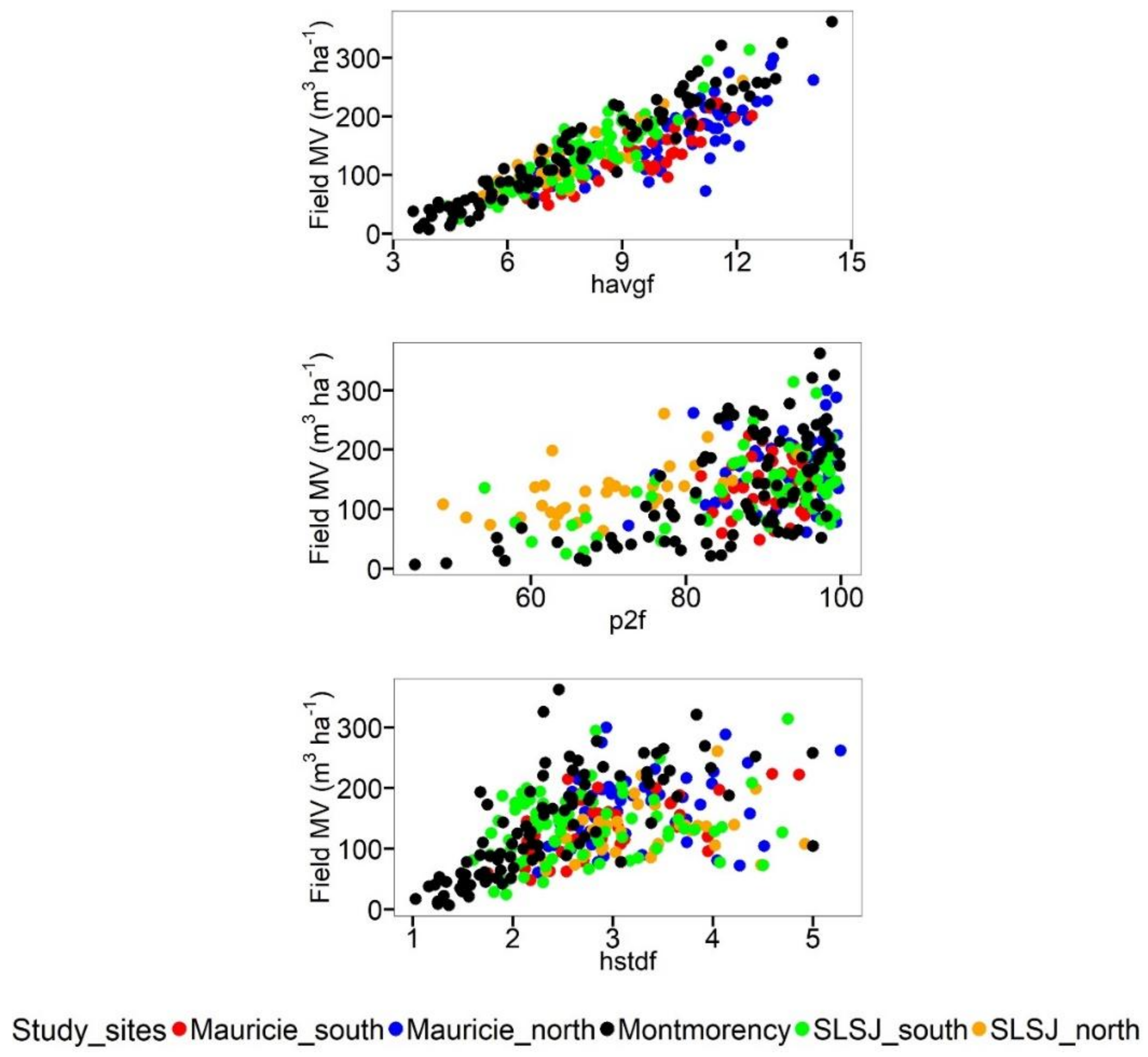
A crucial step in building the MV models was the search of optimal explanatory variables. The combination of havgf, p2f and hstdf provided the best subset of variables. The addition of a growth adjustment function improved the model significantly (p-value < 0.0001). This function accounted for the MV growth that occurred during the temporal discrepancy. It also enabled us to accurately combine the different lidar datasets. It included a height variable (havgf) as the effect of time on merchantable volume varies with the stand development stage. This result confirms the need to adjust predictive models when temporal discrepancies occur [35].

Models 4 and 6b were the best candidate models. Model 4 contained a site random coefficient (${\mathsf{\Delta }}_{\mathrm{m}}$) accounting for the variability amongst sites. The model performed as efficiently as Model 3, which contained several coefficient adjustments (p-value = 0.9913). This result showed that a local adjustment of canopy height was therefore enough to account for the variability amongst sites. This can be explained by the fact that the correlation between the MV and havgf was high compared to the other explanatory variables (Figure 2). It was of 0.87 versus 0.41 for p2f and hstdf. Modifying havgf only would, therefore, have a comparable effect to modifying all the model parameters.

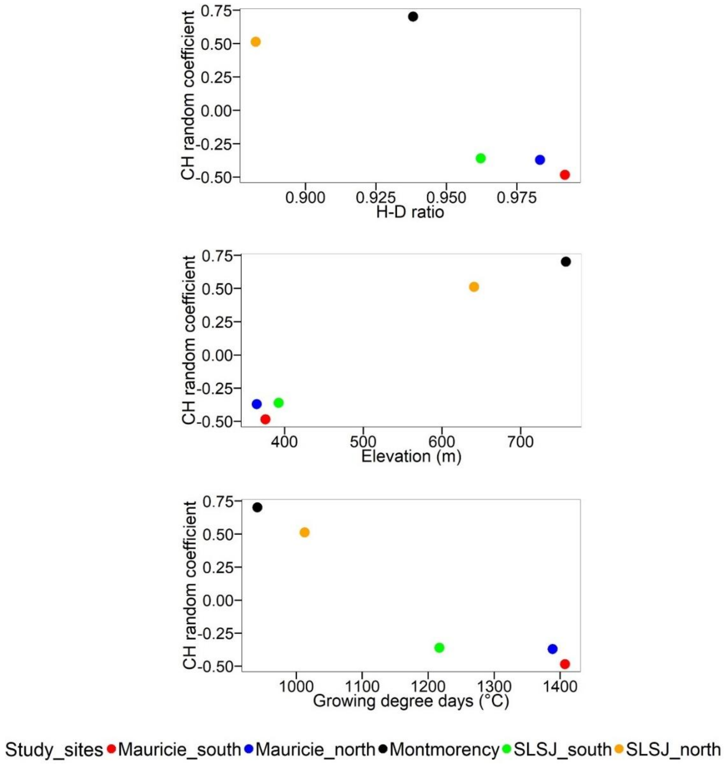
Model 4 random coefficients varied with the characteristics of the study sites: they were positive at the Mauricie_south, Mauricie_north and SLSJ_south sites and negative at the Montmorency and the SLSJ_north sites. The Mauricie_south, Mauricie_north and SLSJ_south sites also had higher H–D ratios (H–D = 0.99, 0.98, 0.96; Table 1) compared to the Montmorency and the SLSJ_north sites (H–D = 0.94 and 0.88). Thinner stems are characterized by higher H–D ratios and have lower merchantable volumes. For a given height, trees were therefore possibly thinner at the Mauricie_south, Mauricie_north and SLSJ_south sites compared to the Montmorency and the SLSJ_north sites. For a given average height, canopy density and canopy structural heterogeneity, havgf needed to be decreased at the Mauricie_south, Mauricie_north and SLSJ_south sites and increased at the Montmorency, SLSJ_north sites when predicting the MV with the same equation.

Table 1 shows a gradient of bioclimatic factors amongst study sites: higher temperatures and gdds were observed at the Mauricie_south, Mauricie_north and SLSJ_south sites compared to the Montmorency and SLSJ_north sites. The random coefficient values (Models 5a and 5b) decreased substantially when a bioclimatic variable was added to the canopy height parameter. This result suggests a correlation between the site variability and the bioclimatic gradient in this case study. The fixed-effect Model 6b which included the elevation variable had a similar prediction accuracy to Model 4 but a lower AIC value. The relationship between the environmental conditions of a study area and the canopy structure variability has also been assessed in other studies [2,36]. Gdd is an indicator of accumulated heat and can be correlated with tree growth [37]. Warmer temperatures and longer growing seasons have a positive effect on tree height growth [38] as well as lower elevations [39]. Trees will, therefore, have a higher H–D ratio and a lower merchantable volume for a given height. Conversely, lower gdds or higher elevations have a negative effect on tree height growth. Trees will have a lower H–D ratio and a higher merchantable volume for a given height. The H–D ratio was smallest at the SLSJ_north site and Montmorency sites.

The canopy variability may be due to other factors such as tree mortality, fire disturbance, site species composition, lidar sensor settings, return density, etc. Sites were composed of similar species, predominantly balsam fir and spruce (Table 1). We tested Models 4 and 6b on a sample of field plots where the proportion of balsam fir was > 60% (256 plots). We obtained similar MV predictions (pseudo-R² = 0.87 and 0.86; RSD = 24.4 m³ ha⁻¹ and 24.5 m³ ha⁻¹ respectively). We, therefore, considered that the species composition had little effect on the MV predictions in this case study.

Several studies have also demonstrated that the lidar settings can have an effect on the precision of derived forest attributes [40,41,42]. The lidar data were acquired separately and with variable acquisition settings in this case study (Table 2). We could not analyze the settings’ effects on the MV models as we did not have enough datasets to draw conclusions. However, their effects would likely be minor compared to the bioclimatic gradient, which had a direct effect on the MV. Further research should be done on this issue.

Our study has several practical uses in an operational context. It suggests flexible models to predict the merchantable volume in study sites where spatial and temporal variabilities are observed. The proposed models are adaptable enough to combine lidar datasets acquired at different time periods. They can accurately predict the merchantable volume both at local (site-specific) and large-scale levels (multiple sites). Using a random coefficient model, such as Model 4, is more advantageous than building several local lidar-based models when predicting forest attributes at a large-scale level. When the variability amongst sites is related to a bioclimatic gradient, a simpler fixed-effect model, such as Model 6b, could then be used with a similar prediction accuracy. The fixed-effect models offer the advantage to be generalizable to other sites of known gdd/elevation, even when field inventory has not been done. As lidar data will be available for the entire province of Quebec by 2021, new lidar study sites could be tested to confirm the relationship between the bioclimatic gradient and the MV variation. The data could also be combined with satellite data to predict the MV at large scale [43,44].

5. Conclusions

Canopy structure variations can be caused by natural forest dynamics occurring over time or by variations of bioclimatic factors (including temperature and elevation). We tested a lidar-based model to predict the merchantable volume (MV) of balsam fir sites located along a bioclimatic gradient of temperature and elevation. Temporal discrepancies up to three years also existed between the field inventory and the lidar data acquisitions. A random coefficient model was adjusted to include a random canopy height coefficient (accounting for site variability) and a growth function (accounting for growth during the temporal discrepancy). The pseudo-R² was of 0.86 and the RSD of 24.3 m³ ha⁻¹. The model performed as efficiently as a model with adjustments on all the parameters (p-value = 0.9913). The site variability was found to be related to the bioclimatic gradient. Fixed-effect models built with bioclimatic variables produced similar prediction accuracies (pseudo-R² = 0.86, RSD ≤ 24.5 m³ ha⁻¹). The effects of site variability, bioclimatic gradients, and temporal discrepancies were found to be essential to generalized lidar-based modelings.

References

1. Boucher, D.; de Grandpré, L.; Gauthier, S. Development of a tool for classifying forest stand structure and comparison of two black spruce forest regions in Quebec. For. Chron. 2003, 79, 318–328. [Google Scholar] [CrossRef]
2. Hansen, A.J.; Phillips, L.B.; Dubayah, R.; Goetz, S.; Hofton, M. Regional-scale application of lidar: Variation in forest canopy structure across the southeastern US. For. Ecol. Manag. 2014, 329, 214–226. [Google Scholar] [CrossRef]
3. Laflèche, V.; Bernier, S.; Saucier, J.-P.; Gagné, C. Indices de Qualité de Station des Principales Essences Commerciales en Fonction des Types Écologiques du Québec Méridional—Site Indices of the Main Commercial Species Following the Ecological Types of Southern Quebec; Gouvernement du Québec, Ministère des Ressources naturelles, Direction des inventaires forestiers Québec: Ville de Québec, QC, Canada, 2013; p. 115. [Google Scholar]
4. McRoberts, R.E.; Tomppo, E.O. Remote sensing support for national forest inventories. Remote Sens. Environ. 2007, 110, 412–419. [Google Scholar] [CrossRef]
5. Magnussen, S.; Eggermont, P.; LaRiccia, V.N. Recovering tree heights from airborne laser scanner data. For. Sci. 1999, 45, 407–422. [Google Scholar]
6. Maltamo, M.; Packalén, P.; Yu, X.; Eerikäinen, K.; Hyyppä, J.; Pitkänen, J. Identifying and quantifying structural characteristics of heterogeneous boreal forests using laser scanner data. For. Ecol. Manag. 2005, 216, 41–50. [Google Scholar] [CrossRef]
7. White, J.C.; Coops, N.C.; Wulder, M.A.; Vastaranta, M.; Hilker, T.; Tompalski, P. Remote sensing technologies for enhancing forest inventories: A review. Can. J. Remote Sens. 2016, 42, 619–641. [Google Scholar] [CrossRef]
8. Bouvier, M.; Durrieu, S.; Fournier, R.A.; Renaud, J.-P. Generalizing predictive models of forest inventory attributes using an area-based approach with airborne LiDAR data. Remote Sens. Environ. 2015, 156, 322–334. [Google Scholar] [CrossRef]
9. Næsset, E. Predicting forest stand characteristics with airborne scanning laser using a practical two-stage procedure and field data. Remote Sens. Environ. 2002, 80, 88–99. [Google Scholar] [CrossRef]
10. Treitz, P.; Lim, K.; Woods, M.; Pitt, D.; Nesbitt, D.; Etheridge, D. LiDAR sampling density for forest resource inventories in Ontario, Canada. Remote Sens. 2012, 4, 830–848. [Google Scholar] [CrossRef]
11. Yoga, S.; Bégin, J.; St-Onge, B.; Gatziolis, D. Lidar and multispectral imagery classifications of balsam fir tree status for accurate predictions of merchantable volume. Forests 2017, 8, 253. [Google Scholar] [CrossRef]
12. Nord-Larsen, T.; Schumacher, J. Estimation of forest resources from a country wide laser scanning survey and national forest inventory data. Remote Sens. Environ. 2012, 119, 148–157. [Google Scholar] [CrossRef]
13. Næsset, E. Airborne laser scanning as a method in operational forest inventory: Status of accuracy assessments accomplished in Scandinavia. Scand. J. For. Res. 2007, 22, 433–442. [Google Scholar] [CrossRef]
14. Næsset, E.; Gobakken, T. Estimation of above-and below-ground biomass across regions of the boreal forest zone using airborne laser. Remote Sens. Environ. 2008, 112, 3079–3090. [Google Scholar] [CrossRef]
15. Nilsson, M.; Nordkvist, K.; Jonzén, J.; Lindgren, N.; Axensten, P.; Wallerman, J.; Egberth, M.; Larsson, S.; Nilsson, L.; Eriksson, J. A nationwide forest attribute map of Sweden predicted using airborne laser scanning data and field data from the National Forest Inventory. Remote Sens. Environ. 2017, 194, 447–454. [Google Scholar] [CrossRef]
16. MRN. Vegetation Zones and Bioclimatic Domains in Quebec; Ministère des Ressources Naturelles, Direction des Inventaires Forestiers: Québec, QC, Canada, 2001. [Google Scholar]
17. MFFP. Données Descriptives des Placettes-Échantillons Temporaires - Descriptive Data of the Temporary Sample Plots; Ministère des Forêts, de la Faune et des Parcs, Direction Des Inventaires Forestiers: Québec, QC, Canada, 2016.
18. MFFP. Guide d’utilisation des Produits Intégrés de l’inventaire écoforestier du Québec Méridional - User Guide of the Southern Quebec Ecoforest Inventory Database; Ministère des Forêts, de la Faune et des Parcs, Direction des Inventaires Forestiers, Gouvernement du Québec: Québec, QC, Canada, 2017; p. 47.
19. Régnière, J.; Saint-Amant, R.; Béchard, A. BioSIM 10 – User’s Manual; Natural Resources Canada, Canadian Forest Service: Québec, QC, Canada, 2014; LAU-X-137E; p. 72. [Google Scholar]
20. Bégin, J.; Raulier, F. Comparaison de différentes approches, modèles et tailles d’échantillons pour l’établissement de relations hauteur-diamètre locales—A comparison of different methods, models and sample sizes for the establishment of local height-diameter relationships. Can. J. For Res. 1995, 25, 1303–1312. [Google Scholar] [CrossRef]
21. Sumida, A.; Miyaura, T.; Torii, H. Relationships of tree height and diameter at breast height revisited: Analyses of stem growth using 20-year data of an even-aged Chamaecyparis obtusa stand. Tree Physiol. 2013, 33, 106–118. [Google Scholar] [PubMed]
22. Fortin, M.; DeBlois, J.; Bernier, S.; Blais, G. Mise au point d’un tarif de cubage général pour les forêts québécoises: une approche pour mieux évaluer l’incertitude associée aux prévisions - Establishing a general cubic volume table for Québec forests: an approach to better assess prediction uncertainties. For. Chron. 2007, 83, 754–765. [Google Scholar]
23. Isenburg, M. “LAStools-Efficient LiDAR Processing Software” (Version 150526, Unlicensed). Available online: http://rapidlasso.com/LAStools (accessed on 1 August 2017).
24. McGaughey, R.J. FUSION/LDV: Software for LIDAR Data Analysis and Visualization; Version 3.42; US Department of Agriculture, Forest Service, Pacific Northwest Research Station: Seattle, WA, USA, 2014; p. 175. [Google Scholar]
25. Yoga, S.; Bégin, J.; St-Onge, B.; Riopel, M. Modeling the effect of the spatial pattern of airborne Lidar returns on the prediction and the uncertainty of timber merchantable volume. Remote Sens. 2017, 9, 808. [Google Scholar] [CrossRef]
26. Pothier, D.; Savard, F. Actualisation des Tables de Production pour les Principales Espèces Forestières du Québec—Yield Tables Updates for The Main Forest Species of Quebec; Ministère des Ressources Naturelles: Québec, QC, Canada, 1998; p. 183. [Google Scholar]
27. Longford, N.T. Random coefficient models. In Handbook of Statistical Modeling for the Social and Behavioral Sciences; Springer: New York, NY, USA, 1995; pp. 519–570. [Google Scholar]
28. Pinheiro, J.; Bates, D. Mixed-Effects Models in S and S-PLUS; Springer-Verlag: New York, NY, USA, 2000. [Google Scholar]
29. Pinheiro, J.; Bates, D.; DebRoy, S.; Sarkar, D.; R Core Team. nlme: Linear and Nonlinear Mixed Effects Models. R Package Version 3.1–117. 2014. Available online: http://CRAN. R-project. org/package= nlme (accessed on 21 March 2018).
30. R Core Team. R: A Language and Environment for Statistical Computing; R Foundation for Statistical Computing: Vienna, Austria, 2017. [Google Scholar]
31. Refaeilzadeh, P.; Tang, L.; Liu, H. Cross-validation. In Encyclopedia of Database Systems; Springer: Berlin, Germany, 2009; pp. 532–538. [Google Scholar]
32. Breidenbach, J.; Kublin, E.; McGaughey, R.; Andersen, H.-E.; Reutebuch, S. Mixed-effects models for estimating stand volume by means of small footprint airborne laser scanner data. Photogramm. J. Finl. 2008, 21, 4–15. [Google Scholar]
33. Kotivuori, E.; Korhonen, L.; Packalen, P. Nationwide airborne laser scanning based models for volume, biomass and dominant height in Finland. Silva Fenn. 2016, 50. [Google Scholar] [CrossRef]
34. Suvanto, A.; Maltamo, M. Using mixed estimation for combining airborne laser scanning data in two different forest areas. Silva Fenn. 2010, 44, 91–107. [Google Scholar] [CrossRef]
35. Bright, B.C.; Hudak, A.T.; McGaughey, R.; Andersen, H.E.; Negrón, J. Predicting live and dead tree basal area of bark beetle affected forests from discrete-return lidar. Can. J. Remote Sens. 2013, 39, S99–S111. [Google Scholar] [CrossRef]
36. Ashiq, M.W.; Anand, M. Spatial and temporal variability in dendroclimatic growth response of red pine (Pinus resinosa Ait.) to climate in northern Ontario, Canada. For. Ecol. Manag. 2016, 372, 109–119. [Google Scholar]
37. McMaster, G.S.; Wilhelm, W. Growing degree-days: one equation, two interpretations. Agric. For. Meteorol. 1997, 87, 291–300. [Google Scholar] [CrossRef]
38. Fortin, M.; Bernier, S.; Saucier, J.-P.; Labbé, F. Une Relation Hauteur-Diamètre Tenant Compte de L’influence de la Station et du Climat Pour 20 Espèces Commerciales du Québec—A Height-Diameter Relationship Which Takes into Account the Influence of the Quality Station and the Climate for 20 Commercial Species in Quebec; Gouvernement du Québec, Direction de la recherche forestière: Québec, QC, Canada, 2009.
39. Coomes, D.A.; Allen, R.B. Effects of size, competition and altitude on tree growth. J. Ecol. 2007, 95, 1084–1097. [Google Scholar] [CrossRef]
40. Ehlert, D.; Heisig, M. Sources of angle-dependent errors in terrestrial laser scanner-based crop stand measurement. Comput. Electron. Agric. 2013, 93, 10–16. [Google Scholar] [CrossRef]
41. Keränen, J.; Maltamo, M.; Packalen, P. Effect of flying altitude, scanning angle and scanning mode on the accuracy of ALS based forest inventory. Int. J. Appl. Earth Observ. Geoinform. 2016, 52, 349–360. [Google Scholar] [CrossRef]
42. Næsset, E. Effects of different sensors, flying altitudes, and pulse repetition frequencies on forest canopy metrics and biophysical stand properties derived from small-footprint airborne laser data. Remote Sens. Environ. 2009, 113, 148–159. [Google Scholar] [CrossRef]
43. Chasmer, L.; Barr, A.; Hopkinson, C.; McCaughey, H.; Treitz, P.; Black, A.; Shashkov, A. Scaling and assessment of GPP from MODIS using a combination of airborne lidar and eddy covariance measurements over jack pine forests. Remote Sens. Environ. 2009, 113, 82–93. [Google Scholar] [CrossRef]
44. Hudak, A.T.; Lefsky, M.A.; Cohen, W.B.; Berterretche, M. Integration of lidar and Landsat ETM+ data for estimating and mapping forest canopy height. Remote Sens. Environ. 2002, 82, 397–416. [Google Scholar] [CrossRef]
Figure 1. Location of the study sites.
Forests 09 00166 g001
Figure 2. Scatter plots of the field merchantable volume (MV) against the explanatory variables. Field plots of each study site are represented by a dot. havgf = average height of first returns above 2 m; p2f = percentage of first returns above 2 m; hstdf = standard deviation of the height of first returns above 2 m.
Forests 09 00166 g002
Figure 3. Scatter plots of Model 4 canopy height (CH) random coefficients plotted against the height–diameter ratio (H–D ratio), the elevation, and the growing degree day variables presented by study site.
Forests 09 00166 g003