Analyzing the Efficiency of a Start-Up Cable Yarding Crew in Southern China under New Forest Management Perspectives

Abstract

This case study analyzed the performance of a start-up cable yarding crew in southern China through operational monitoring by consecutive time studies, long-term log book recordings and efficiency evaluation by stochastic frontier analysis (SFA). The crew, which used a KOLLER K303 H mobile tower yarder, was monitored for two years. During this period, detailed data recordings of 687 yarding cycles of 12 yarding corridors as well as log book recordings of an additional 1122 scheduled system hours (SSH, including all delays) were generated. Mean extraction productivity of the system ranged between 5.23 and 6.40 m³ per productive system hour (PSH₀, excluding all delays), mostly depending on slope yarding distance and lateral distance. Corresponding gross-productivity ranged from 1.91 to 2.24 m³/SSH, with an overall mean machine utilization rate of 31%. Unproductive yarding times and delays associated with the relative low utilization rate were mainly caused by lengthy rigging processes, as well as organizational deficiencies and not yet fully developed skill sets of the operating crew. The latter was reflected in a mean efficiency effect frontier value of 0.62 based on evaluation of data sets of individual yarding cycles recorded during detailed assessments, suggesting a mean improvement potential of 38% based on the SFA, translating in a potentially achievable gross-productivity of 2.64 to 3.09 m³/SSH. We conclude that current local operating conditions including insufficient planning, implementation and logistics and in particular, frequent discontinuations of system operations of up to three months all resulting in generally low operation hours per shift and per year, inhibit efficient operations and rapid skill development. These circumstances also inhibit an economic utilization of the equipment. Nevertheless, from a technical perspective, yarding systems have a promising potential in southern China.

1. Introduction

With its high processing capacities and steadily growing domestic consumer demand, China has become a significant contributor to the global forest products market but is also facing a challenging situation in terms of raw material supply [1]. After years of intensive forest exploitation and resource depletion, China has implemented various national forest policy reform programs in order to conserve its remaining natural forests and to promote raw material supply from extensively established plantation forests, an example of which are the national level’s Six Key Forestry Programs (SKFP) [2,3]. In addition, multiple use forestry was propagated to preserve biodiversity and enhance forest ecosystem services [3]. Though China was able to consistently increase its plantation area over the past years, the productivity of the plantations has remained low and its management failed to provide the required raw material in an efficient way [4]. This situation contributed to an elevated demand-and-supply gap of raw material and caused a high dependency on roundwood imports, which are already worth USD 10 billion annually and constitute China’s third largest foreign exchange commodity after oil and steel [1].

Mechanization efforts of forest operations will play a fundamental role in China’s ambitions to increase the productivity of its plantation based forestry, as was the case recently in Brazil’s emerging forest industry [5]. Currently, timber harvesting operations in China heavily depend on a manual workforce. Likely, this has to change in the future because of increasing wages and a lower availability of formerly abundant migrant workers, which have been the backbone of this form of management [1]. These manual operations will also not be capable of meeting market demand for domestically produced sawlogs of larger dimensions due to the physical inability to manually handle logs with large diameters, particularly during the extraction process, as was revealed by Engler [6]. Furthermore, due to limited land availability, forest plantations are often located on less favorable sites such as steep terrain. In such areas, the objective of growing larger tree dimensions through periodic thinnings [7] requires a suitable extraction technique, in order to ensure efficient, safe and ergonomic operations that reduce impact on soil and residual trees [3]. Cable yarding systems are known to be more suitable for wood extraction in steep terrain with lower soil disturbance compared to ground based extraction systems due to their load suspension and lower forest road density requirements [8]. This is particularly beneficial with respect to China’s low level of logging infrastructure (e.g., low density of truck roads, unfavorable road location in valleys adjacent to streams), [4]. Under these conditions, standing skyline systems with slack-pulling carriages are considered to be very suitable for medium to long extraction distances. Compared to running skyline systems, these systems allow for controlled lateral yarding which is of particular importance in thinning operations in order to minimize damage to residual trees [9]. However, cable yarding operations require strategic planning and professional operating personnel, prerequisites that are currently not fully fulfilled for forest operations in China, particularly in the vast plantation areas of the southern provinces [6,10].

This study evaluates the performance of a start-up cable yarding crew in southern China over a period of two years. The monitored crew was the first in this region to use a standing skyline system (mobile tower yarder) for timber extraction during thinning operations. More specifically, the objectives of this study are: (1) to analyze and evaluate indicators for performance improvement of a professionally trained start-up crew over time by combining different monitoring approaches; (2) to identify factors hindering full performance with respect to work execution and operational management; (3) to evaluate the overall suitability of standing skyline systems and associated operational challenges to meet the demands of local forest management schemes. An integral discussion of the findings in subsequent research may help to define basic requirements for efficient cable yarding operations and other mechanized harvesting operations in southern China.

2. Materials and Methods

2.1. Study Site

The study was conducted in collaboration with the Experimental Center of Tropical Forestry (ECTF), a regional research institute in southern China, affiliated to the Chinese Academy of Forestry. It is located close to the Vietnamese border in Pingxiang (22°05′49′′ N; 106°45′24′′ E), Guangxi Zhuang Autonomous Region. The regional climate is subtropical with an annual mean temperature of 22.1 °C and a mean precipitation of 1227 mm. Approximately two thirds of precipitation occur during a distinct rainy season from May to September [11]. During the four data collection campaigns—autumn 2013 (campaign A), spring 2014 (campaign B), autumn 2014 (campaign C) and spring 2015 (campaign D)—dry periods with temperatures ranging from 20 °C to 30 °C were chosen, which represent typical conditions of timber harvesting operations in Guangxi. Forest plantations in Guangxi are dominated by pine (Pinus massoniana Lamb.) and eucalyptus (Eucalyptus grandis x E. urophylla). These plantations are primarily managed in short rotation clearcut systems producing small diameter logs for fiber generation and wood based panel production. Commonly, after the trees are felled and delimbed in the stand, they are cross-cut onsite into logs 2 m in length and manually extracted to the next feeder road that is suitable for small farm trucks [6].

The ECTF manages 19,000 ha of plantation forests, with pine being the dominating species. Besides conventionally managed sites using the clearcut system, the ECTF is also shifting its attention towards continuous cover forestry for implementing multiple use forestry which favor the production of larger diameter logs through selective cutting and thinning. This new management concept requires new approaches for timber harvesting and extraction. In order to assess the suitability of cable yarding extraction systems in this respect, prescribed thinning stands of pine with DBH (diameter at breast height) of 20 cm and beyond were selected for the experiment. All selected stands were located on the Baiyun forest farm lands and had relatively short extraction corridors (<200 m) and fair slopes (<50%) (

Table 1. Stand Descriptions of Test Sites at Baiyun Forest Farm. Stand Parameters are based on Inventory Data Provided by ECTF, All Stands Consisted of Pine, Stocking on Lateritic Red Soils, Established by Planting at an Initial Spacing of 2 m × 2 m and Stocking of 2500 Trees/Ha. All Operations Were 2nd Thinnings With Uphill Yarding Direction. Standard Deviations in Parenthesis.

Stand parameter	Campaign A	Campaign B	Campaign C	Campaign D
Compartment No.	14	14	54 & 56	55
Weighted mean slope (%)	42	41	33	48
Stand age at time of operation (year)	25	24	20	19
Estimated standing volume (m3) *s.o.b./ha	301	249	186	196
Mean DBH (cm) prior operation	30.7 (±5.4)	28.2 (±4.8)	24.6 (±4.5)	25.3 (±5.1)
Mean top height (m) prior operation	17.5 (±1.8)	17.2 (±1.9)	16.8 (±0.8)	16.5 (±1.1)
Estimated pre-operation stocking (n/ha)	516	516	518	525
Thinning intensity of stem number (%)	45	45	43	35
Mean corridor length (m)	103 (±16.9)	75 (±4.2)	188 (±63.5)	83 (±9.5)

*s.o.b. = solid over bark.

).

Subject to administrative constraints related to the Chinese logging permit issuing process (see [12]), the test sites were selected as to be comparable in terms of stand conditions, management objectives and an uphill yarding direction. Harvesting intensity and individual tree selection were determined by ECTF silviculturists.

2.2. Harvesting System

A semi-mechanized harvesting system was adapted to local conditions (Figure 1). This system included manual tree felling, delimbing and initial bucking of the stem into 2 m multiples (max. 6 m stem lengths) in the stand by one feller using a chainsaw. The tree felling occurred prior to the yarding operation and was not covered by the time and motion studies. Logs were extracted with the cable yarder from the felling site to the yarder’s log deck from where the logs were moved to the landing by a tracked knuckle boom loader. Cross-cutting into the final log lengths of 2 m was executed at the landing by an additional chainsaw operator, prior to loading the logs into farm trucks with the knuckle boom loader. Alternatively to the use of the loader, especially in operations with very small diameter logs, logs were manually manipulated at the landing and loaded onto trucks as described by Engler [6]. Within this study, all logs were manipulated at log deck and landing by a 6 t, domestically manufactured knuckle boom loader (JG-608, Jingli Engineering Machinery Co. Ltd., Quanzhou, Fujian, China). For the study presented here, the yarding process with the KOLLER K303 H (KOLLER Forsttechnik GmbH, Schwoich, Austria) cable yarder was of special interest and therefore monitored and analyzed by time and motion studies.

The KOLLER K303 H (Figure 2), with a standing skyline length of up to 420 m, is a small range, trailer based, mobile tower yarder complemented by the automatic, hydraulic carriage USKA 1.5 (KOLLER Forsttechnik GmbH, Schwoich, Austria) for payloads up to 1.5 t. The yarder can be rigged for gravity based uphill yarding (two cable system), as well as for all-terrain operations with a haulbackline (three cable system) (

Table 2. Technical Description of the KOLLER K303 H Cable Yarder.

Component	Description
System	3-drum, all-terrain, tilt tower yarder (standing skyline)
Drive	4-cylinder diesel engine (64 kW), hydrostatic drive of all winches
Tower	Lattice tower, 7.2 m (with optional extension 8.4 m)
Guylines	4 × 30 m, Ø 16 mm
Skyline	420 m, Ø 14 mm, line pull of 44 kN (at tensioning compartment)
Mainline	400 m, Ø 9.5 mm, line pull of 18 kN (at mid-drum diameter)
Haulbackline	800 m, Ø 10 mm, line pull of 18 kN (at mid-drum diameter)
Carriage	Slack-pulling carriage with hydraulic clamps, payload of 1.5 t (tare: 345 kg)
Choker system	conventional Bardon choker (4×)

). Due to its relatively simple operation, moderate purchase price and rugged design, the yarder has been very popular in different parts of the world for over three decades and is commonly applied in thinnings (see [8,14]).

2.3. Trial Crew

As soon as the purchase of the yarder was completed in 2013, the cable yarder operating crew was recruited from the region by ECTF, with a preference for people used to working in the forest environment and who had a fair understanding of mechanics. The crew attended a two week training program specifically designed for beginners, delivered by foreign cable yarding experts and a technical instructor of the yarder manufacturer. The course covered theoretical and practical aspects of cable yarding operations with a special focus on the K303 H. Follow-up training was conducted after six months of system operation. Besides ensuring safe and efficient operation of the yarder, the second course also conveyed the principles of downhill yarding. Additionally, after every field campaign, a brief review of observed operation performance was conducted by the two time keepers (S.H. and S.S.) in order to improve overall system performance.

2.4. Time and Motion Studies

To determine the principal performance of the crew at designated periods of investigation, elemental time studies were conducted during the field campaigns between 2013 and 2015. This was done through two interacting, radio-wired time keepers with digital stop watches following the elemental snap back timing method and applying IUFRO standard work study nomenclature [15]. Time keeper 1 was located at the log deck, while time keeper 2, together with an assistant, monitored the choker setters in the stand. Both time keepers individually and independently timed the attributed cycle elements (

Table 3. Description of Cycle Elements of the Yarding Cycle.

Cycle Element	Description
Outhaul	Begins when the operator releases the mainline break (touching the lever) and starts to move the carriage from the log deck to the designated in stand position of the choker setter. It ends as soon as the mainline is lowered from the carriage and either the choker setter touches the choker, or, in case of delay, the choker touches the ground
Lateral Outhaul	Begins with the end of the Outhaul and ends when the choker setter reaches the first log, as soon as he stops his forward movement in order to Hook Up
Hook Up	Begins at the end of Lateral Outhaul and ends when all logs are hooked, as soon as the choker setter gives the signal to the operator to wind up the mainline for Lateral Inhaul
Lateral Inhaul	Begins at the end of Hook Up and ends as soon as the choker setter releases the skyline clamps
Inhaul	Begins at the end of Lateral In and ends as soon as the skyline clamps are engaged at landing
Unhooking	Begins at the end of Inhaul and ends after the mainline brake is released to start the Outhaul

) against a measured continuous time for reference. During campaign B, not all cycles of the prepared corridors were measured directly in the field due to a lengthy interruption of the operation by an unexpectedly long rainy period and time constraints of the time keepers. However, measurements of the continued operation were complemented through videotaping by the Chinese partners. The video tapes were later analyzed by the time keepers in a professional video editing room, using Adobe Premiere Pro CC (Adobe Systems Software Ltd., Dublin, Ireland).

Delay free net-cycle times are referring to productive system hours (PSH₀), i.e., exclusively based on productive work time. Non-work times and supportive work times (further on, both together, denoted as delay times) are separated from these. Delay-free and delay times sum up to gross-cycle times and refer to scheduled system hours (SSH) which include productive and non-productive work times (but exclude official meal and rest times) in order to calculate the machine utilization rate (MU) (Equation (1)). Machine utilization was separated in shift utilization (MU_Total), accounting for the complete work day and operation utilization (MU_Operation), accounting for the time of actual yarding. This approach was chosen in order to distinguish planning and organizational deficits from actual machine operation deficits. Following IUFRO terminology [15], measured times have been categorized in the following main classes: productive work time (PW; directly related to PSH₀), preparatory time (PT), rest and personal time (RP), disturbance time (DT), interference time (IT), maintenance time (MT) and repair time (RT). Since the DT is only linked to the data collection and implementation of the research, these times have been removed from the data set during the analysis and were not accounted for in the shift times.

$$\text{MU}= \frac{{\text{PSH}}_0}{\text{SSH}}\times 100$$

(1)

where:

• MU = machine utilization rate (%)
• PSH₀ = productive system hours (h)
• SSH = scheduled system hours (h)

Since the work place times PT, RP, IT, MT and RT interrupt the wood extraction work process and account for delays and other non-productive times, a delay factor was calculated in percent of PSH₀ (Equation (2)) for each of the mentioned work place times individually. This allows specific comparisons between work cycles and campaigns, rather than only providing the aggregated utilization rate. These were summed up to a total delay factor (Equation (3)), to allow for a better comparison between the individual data sets, following the approach recommended by Spinelli and Visser [16]. Besides the delay classification according to work place time category, individual delay events have been defined on observation (e.g., the IT categorized individual delay event “log hang up”), to identify the most frequently occurring disturbances of the operations.

$${\text{DF}}_x= \frac{h_x}{{\text{PSH}}_0} \times 100$$

(2)

where:

• DF_x = delay factor of delay category x (%)
• h_x = sum of all delay times of delay category x (h)
• PSH₀ = productive system hours (h)

$${\text{DF}}_{\text{Total}} ={ \text{DF}}_{\text{PT}}+{ \text{DF}}_{\text{RP}}+{ \text{DF}}_{\text{IT}}+{ \text{DF}}_{\text{MT}}+{ \text{DF}}_{\text{RT}}$$

(3)

where:

• DF_Total = total delay factor (%)
• DF_PT = delay factor preparatory times (%)
• DF_RP = delay factor rest and personal times (%)
• DF_IT = delay factor interference times (%)
• DF_MT = delay factor maintenance times (%)
• DF_RT = delay factor repair times (%)

In preparation of the elemental time study, all logs along each designated yarding corridor were given a unique log ID-number in order to assign individual logs to a yarding cycle later on. Furthermore, the log dimensions were measured and recorded with their felling direction and location in the corridor. The individual log volumes were determined by the SMALIAN formula, using the mean of the basal areas at both ends of the log, multiplied by its length [17]. Terrain slope, slope yarding distances (henceforth referred to yarding distance) and corridor widths have been measured and marked at regular intervals with flagging tape and spray paint on residual trees. During the yarding operation, lateral yarding angles were determined with a compass and lateral and yarding distances were estimated for each cycle by time keeper 2 and his assistant, with reference to the flagging. Additionally, a degree of hindrance by ground vegetation was assigned through a subjectively rated scale of: 1, none; 2, normal; 3, heavy. In the same way, the log presentation quality by the felling team was assigned with respect to correct felling direction, bucking, delimbing and slash handling as classes: 1, good; 2, fair; 3 poor and recorded accordingly. These variables have been complemented by the corridor specific slope and off-set slope angle and treated as independent variables.

Net-cycle and elemental time equations based on delay free productive times have been modeled through step-wise multiple linear regressions, following standard procedures [18], using the software package SPSS 22 (IBM Corp., Amonk, NY, USA). Extreme values of the independent variables (yarding distance, lateral distance, lateral angle, log volume, number of logs, slope, off-set slope, vegetation class and log presentation quality) outside three times the standard deviations were removed before model generation (after checking for plausibility, e.g., originating from false field form transfers). In stepwise regression, individual independent variables are either entered or removed based on their F-probability (alpha-to-enter: α < 0.05 and alpha-to-remove: α > 0.10) to explain the dependent variable. The final model is generated as soon as no other independent variables can be considered for further inclusion. Subsequently, validity of the model was checked by the standardized residues (normal distribution) and collinearity diagnostics (condition index < 30).

2.5. Long Term Recordings

Elemental time studies are most suitable in understanding functional steps and to identify inefficiencies of work processes in detail due to their very discriminating approach [19]. However, such studies are very limited in estimating long-term trends and particularly large delays are inadequately analyzed with respect to overall performance impact [20]. Since the objective of this study was to evaluate the crew’s performance during the start-up phase of the newly introduced yarding system, as a supplement to the detailed but timewise very limited elemental time study, a less detailed shift-level study [19] based on log book recordings, was performed as well. The log book recordings covered the entire time frame during and between the field campaigns. This long-term monitoring of the operations included two ways of recording: first of all, the yarder operator recorded the actual duration of each operation through the machine’s hour meter gauge, differentiating between rigging (e.g., during skyline out-spool) and yarding (actual machine use) activities and assigning a corridor specific ID to each data set. Furthermore, he recorded the measured major delay times and cycle numbers for each shift, the latter clocked with a mechanical hand counter. Due to the less detailed recordings in the log book, time classifications needed to be adapted accordingly. Therefore, within the long-term records, PSH₁₅ is considered as work-related productive time, which includes PT, RP, DT, IT, MT and RT up to 15 min and only major delays and non-productive times beyond the 15 min threshold have been accounted for separately [16].

The second monitoring was done by the operation manager in charge, who recorded detailed information about the individual corridors, yarding direction, corridor length, corridor width, slope, numbers of intermediate supports, rigging times, daily shift length and the estimated yarded volume.

2.6. Efficiency Analysis by Stochastic Frontier Analysis

Established time study and production monitoring methodologies help to quantify output productivity but have only a limited means of evaluating how efficient a system and its associated operation crew were generating this output. In economic terms, frontier production functions are able to rate a firm’s efficiency by using scalar output quantities at given input resources, by approaching an idealized, so-called potential frontier isoquant, as first described by Farrell [21]. His work built the basis for the development of the stochastic frontier analysis (SFA) as independently introduced by Aigner et al. [22] and Meeusen and van Den Broeck [23]; and which was thoroughly described by Kumbhakar and Lovell [24]. Conventional production functions use ordinary least squares (OLS) regression techniques, averaging the production observations through a line of best fit. Yet, since microeconomic theory proposes that a production function should indicate the maximum attainable output quantity for given input quantities, no actual observation could theoretically be above the function and all observations below would be directly associated to technical inefficiency [25]. Within the SFA approach, maximum likelihood estimates within parametric production functions, as in Cobb-Douglas [26] form, model the deviation of the observations from the ideal production frontier to quantify a firm’s technical efficiency [27]. In the case of the efficiency effect frontier (EEF) after Battese and Coelli [28] applied in this research, the ideal frontier isoquant is 1, confirming optimum efficiency and 0, representing no efficiency at all.

Yet the SFA approach was developed to compare different firms in order to rate the individual firm’s performance within a group or sector. Within this study, only one cable yarding crew is the subject of investigation. Since the monitoring of this crew’s skill development and expected corresponding performance improvement is of interest, the SFA approach was adapted by considering every monitored yarding cycle of each associated corridor independently, in lieu of individual firms. Consequently, the sum of all corridors represent the sector to be rated, in order to monitor if the crew is approaching the potential frontier isoquant generated by this sector. This is a different approach to the work of Aaalmo and Baardsen [29], who applied SFA in a cable yarding study as well but compared the various crews, with respect to their daily output generated through productive work time and yarding cycles per day.

Following the mandatory property of a production function with strict compliance to monotonicity—implying that any additional input unit cannot decrease the level of output [30], a production function at cycle level was defined in Cobb-Douglas form based on measureable time study parameters. Production input units could be quantified as work time (cycle time) and material input (logs per cycle), to generate the output product (volume at landing), (Equation (4)).

$$Y_V= A{T}^{\mathsf{\beta }1}{L}^{\mathsf{\beta }2}$$

(4)

where:

• Y_v = volume output per yarding cycle (m³)
• A = total factor productivity parameter
• β1 and β2 = output elasticities
• T = input cycle time (min)
• L = input number of logs yarded per cycle (n)

Within the Cobb-Douglas production functions, coefficients are characterized by associated elasticities in which the responsiveness of output to a changing ratio of input is quantified. The elasticity parameter corresponds to the increased quantity for an additional unit of input and is in sum for all coefficients also expressed by returns to scale [30].

The SFA with an EEF uses a model that applies natural logarithms to a production function of Cobb-Douglas type, complemented with an error coefficient ($v$) accounting for measurement errors and other noise upon the shape and position of the estimated frontier. Further, a term for technical inefficiencies ($u$), caused by operational factors such as yarding distance, vegetation hindrance, log presentation quality or steepness of terrain, which can potentially decrease the production efficiency (Equation (5)) is added as well [25].

$$\ln Y_V={ \mathsf{\beta }}_0+{\mathsf{\beta }}_1\text{ln} T+{\mathsf{\beta }}_2\text{ln} L+v-u$$

(5)

where:

• lnY_v = scalar production output per cycle (EEF)
• lnT = vector of cycle time
• lnL = vector of number of logs
• β₀ = coefficient of total-factor productivity (A)
• β₁ and β₂ = coefficients of the technology parameter to be estimated
• v = two-sided error component
• u = non-negative technical inefficiency component

Distributional assumptions are required for SFA models since these are estimated by econometric likelihood estimations. The noise term $v$ is assumed to follow a normal distribution with zero mean and constant variance (${\mathsf{\sigma }}_v^2$). The inefficiency term $u$ is specified to follow a positive truncated normal distribution with a constant scale parameter (${\mathsf{\sigma }}_u^2$) and a location parameter ($\mathsf{\mu }$) that depends on the additional explanatory variables. In order to quantify the importance of the inefficiency term $u$ over the error term$v$, the estimation algorithm re-parametrizes the variance parameter ${\mathsf{\sigma }}_v^2$ and the scale parameter ${\mathsf{\sigma }}_u^2$ in terms of ${\mathsf{\sigma }}^2={\mathsf{\sigma }}_v^2+{\mathsf{\sigma }}_{u }^2$ and $\mathsf{\gamma }={\mathsf{\sigma }}_u^2/{\mathsf{\sigma }}^2$ and compares the stochastic frontier model with a conventional OLS model through a likelihood ratio test: If γ = 0, the inefficiency term $u$ is irrelevant and the results of the stochastic frontier model should be equal to an OLS model. Yet, if γ = 1, the noise term v is irrelevant and variation from the ideal production function is explained by technical inefficiency too [25].

The SFA and subsequent analysis was conducted with the statistical software R 3.2.2 [31] using the package frontier [32]. The significance level for all analysis conducted in this research was set to α < 0.05.

3. Results

3.1. Elemental Time Study

Over the four field campaigns (

Table 4. System Productivity Parameters as Measured During the Four Field Campaigns. Standard Deviations in Parenthesis.

System Productivity	Campaign A	Campaign B	Campaign C	Campaign D
Observed corridors (n)	3	2	3	4
Observed yarding cycles (n)	183	90	238	176
Mean yarding distance (m)	59.8 (±29.7)	40.5 (±23.4)	114.1 (±64.1)	41.9 (±24.3)
Mean corridor off-set slope line (°)	25.5 (±21.2)	12.9 (±1.0)	20.6 (±2.2)	12.3 (±3.7)
Mean lateral distance (m)	13.3 (±9.7)	19.8 (±9.5)	22.9 (±12.1)	15.4 (±7.5)
Total volume yarded (m3)	100.84	53.44	139.93	94.37
Total shift hours observed (h)	60.46	26.87	72.26	43.49
Average logs per cycle (n)	4.0 (±0.8)	3.6 (±1.2)	3.5 (±1.1)	3.3 (±1.1)
Average volume per load (m3)	0.551 (±0.214)	0.594 (±0.265)	0.588 (±0.253)	0.536 (±0.218)
SSHTotal	52.70	19.05	62.57	38.56
SSHOperation	19.86	10.17	38.04	19.58
PSH0	17.42	8.35	26.77	14.80
m3/SSHTotal	1.91	2.81	2.24	2.45
m3/SSHOperation	5.08	5.25	3.68	4.82
m3/PSH0	5.79	6.40	5.23	6.37

), the trial crew was monitored for about 203 h in total. During that time, detailed time studies on 12 yarding corridors have been conducted, with a total of 687 yarding cycles valid for analysis. The net (m³/PSH₀) and gross (m³/SSH) productivity has been highest during campaign B, representing the campaign with the shortest corridors and also the lowest number of observations. In contrast, campaign C had the lowest net and gross output but owing to the terrain, also the longest corridors and lateral yarding distances. Campaign C also had the highest number of observations. In general, mean lateral yarding distances increased across the first three campaigns, reaching the highest mean value of 22.9 m in campaign C, as mentioned before. Yet, during the last campaign (D), the mean lateral yarding distance dropped down to 15.4 m.

In all four data sets, the Hook Up process was the most time consuming cycle element, contributing to nearly one third of the total cycle time, also having the highest variability of the elements (Appendix

Table A1. Descriptive statistics of the cycle element and total cycle times of the four data collection campaigns. SD = standard deviation.

Cycle Element	Campaign A						Campaign B						Campaign C						Campaign D
	Mean	SD	Min.	Max.	Percentiles		Mean	SD	Min.	Max.	Percentiles		Mean	SD	Min.	Max.	Percentiles		Mean	SD	Min.	Max.	Percentiles
					5th	95th					5th	95th					5th	95th					5th	95th
Outhaul	0.71	0.24	0.01	1.47	0.36	1.04	0.52	0.18	0.01	0.93	0.19	0.85	0.76	0.31	0.08	1.49	0.28	1.28	0.48	0.19	0.01	1.01	0.18	0.80
Lateral Out	0.81	0.40	0.11	2.01	0.20	1.57	0.98	0.51	0.02	2.39	0.22	2.01	1.07	0.57	0.1	4.34	0.28	2.00	0.94	0.39	0.15	2.27	0.27	1.56
Hook Up	1.85	0.67	0.44	4.97	0.98	2.99	1.83	0.81	0.13	4.23	0.53	3.35	1.68	0.76	0.2	4.59	0.48	2.90	1.47	0.67	0.16	3.74	0.37	2.62
Lateral In	0.82	0.44	0.08	2.40	0.30	1.80	1.03	0.47	0.21	3.34	0.39	1.85	0.95	0.39	0.11	2.13	0.40	1.64	0.77	0.29	0.15	1.66	0.33	1.30
Inhaul	0.96	0.38	0.04	2.20	0.45	1.50	0.67	0.31	0.01	1.62	0.23	1.29	1.24	0.55	0.23	2.57	0.39	2.11	0.67	0.32	0.01	1.63	0.21	1.18
Unhooking	0.56	0.24	0.24	1.96	0.28	0.96	0.71	0.23	0.26	1.52	0.39	1.17	0.74	0.24	0.13	1.45	0.39	1.20	0.61	0.20	0.28	1.34	0.34	0.93
Total Cycle Time	6.52	2.04	2.83	14.00	3.64	10.04	5.63	1.45	2.44	9.32	3.32	8.56	6.43	1.63	2.33	12.18	3.90	9.52	4.94	1.09	2.20	7.58	3.28	7.17

). With respect to machine utilization rates (Appendix

Table A2. Utilization rates of the four field campaigns in form of total on-site SSH (MU_Total), scheduled operation SSH (MU_Operation) and the MU_Operetion related total delay factor (DF_Total) and delay category associated delay factors (DF_IT, DF_PT, DF_MT, DF_RP, DF_RT) in percent after Spinelli and Visser [16].

Campaign	MUTotal (%)	MUOperation (%)	DFTotal (%)	DFIT (%)	DFPT (%)	DFMT (%)	DFRP (%)	DFRT (%)
A	30.1	87.7	14.1	11.5	2.1	0.2	0.1	0.2
B	43.9	82.1	21.8	18.4	2.9	0.2	0.3	0.0
C	42.8	70.4	42.1	26.9	8.7	1.7	1.3	3.5
D	38.4	75.6	32.3	22.3	7.7	0.6	1.7	0.0

), MU_Total has been lowest during campaign A in 2013, but it also showed the highest MU_Operation. Campaign C had the lowest MU_Operation value and the highest DF_Total. However, it was also the longest observed period with an increased tendency of technical delays, as confirmed by the highest values for DF_MT and DF_RT (Table A2).

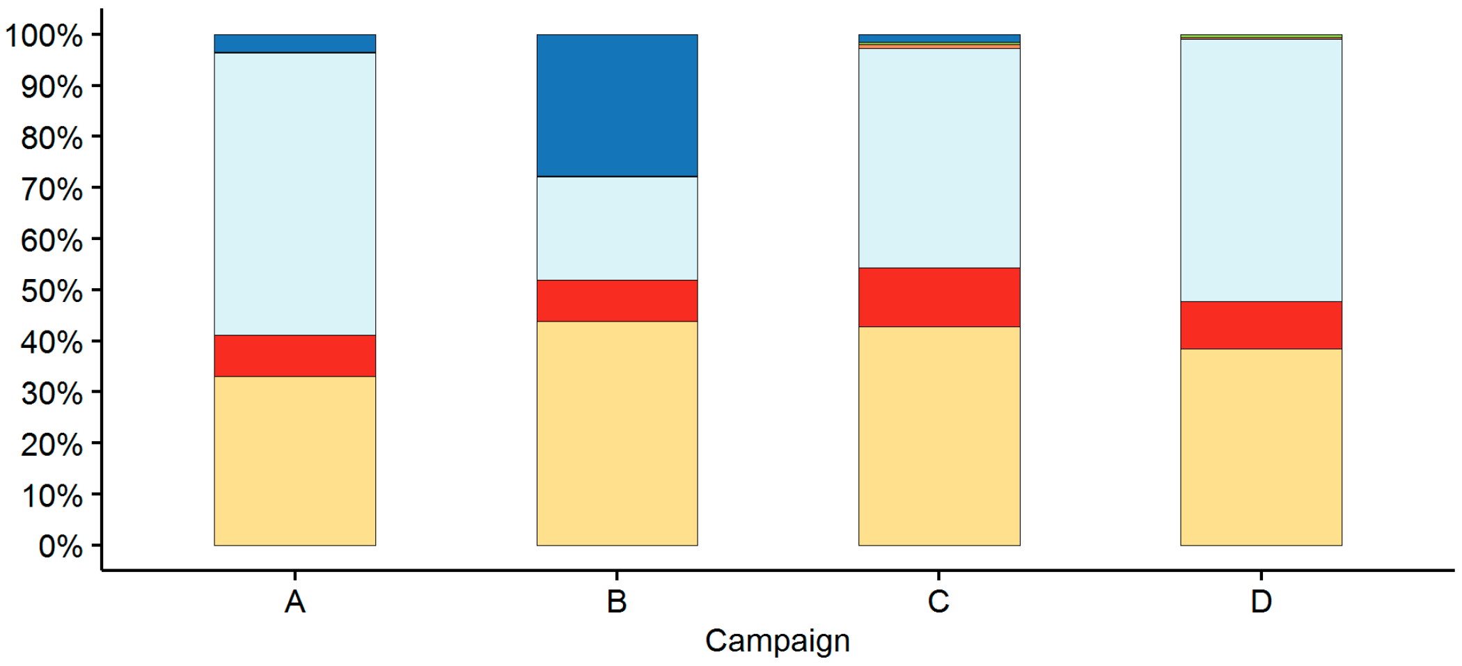
Comparing the productive time (PSH₀) share to non-work times and supportive work times at shift level (SSH_Total), (Figure 3) and at machine operation level (SSH_Operation), (Figure 4) between the campaigns, the high share of PT (preparatory times) on shift level is noticeable, which is mainly due to the preparation process of the yarder and associated rigging. Rigging procedures attributed to corridor installation and take-down have been timed separately and evaluated by applying a suitable European corridor installation times model for small yarders defined by a mainline pull capacity <35 kN, as defined by Stampfer et al. [33] (

Table A3. Modeled and measured corridor installation times for the corridors studied during the field campaigns, the difference between the modeled and measured values as well as the associated corridor attributes.

Corridor	Corridor Length 1 (m)	No. of Intermediate Supports	Installation Times			Take-Down Times
			Measured Time (h)	Modeled 2 Time (h)	Difference (h)	Measured Time (h)	Modeled 2 Time (h)	Difference (h)
1	139	1	9.58	2.38	7.2	2.92	1.94	1.0
2	127	1	6.33	2.36	4.0	3.61	1.89	1.7
3	105	1	4.64	2.32	2.3	not observed
4	75	0	not observed			0.40	2.28	-1.9
5	80	0	2.25	2.28	-0.0	0.97	2.31	-1.3
6	210	2	3.50	2.49	1.0	1.75	1.68	0.1
7	237	1	6.92	2.54	4.4	0.50	2.44	-1.9
8	116	1	3.25	2.34	0.9	1.67	1.84	-0.2
9	67	1	3.30	2.26	1.0	3.55	1.64	1.9
10	76	1	3.40	2.28	1.1	3.50	1.68	1.8
11	90	1	1.25	2.30	-1.1	1.20	1.73	-0.5
12	100	1	1.20	2.31	-1.1	1.28	1.77	-0.5

¹ Corridor length is attributed to the distance from machine tower to tail spar or in case of absence to the tail anchor, representing the theoretical max. carriage travel distance; ² with the model of Stampfer et al. 2006 [33].

).

We are aware of the limited possibility of comparing European conditions in spruce forests of the Austrian Alps, with their longer extraction distances when compared to Chinese pine plantations. But we consider Stampfer’s [33] model appropriate for the purpose in order to compare the Chinese start-up crew with a professional one, particularly with respect to the rigging efforts of the intermediate supports and thereby suggesting a general performance level. It is obvious that during the first corridors in particular, the installation times took much longer than the modeled reference. The very first timed installation took as much as three times as the modelled reference. Later, the measured installation times do not show a clear pattern; installation and take down times being close to the estimated times (e.g., installation of corridor 5) but then at times it was much slower than expected, as observed during installation of corridor 7, while at others were much faster than expected, such as the installation of corridor 11 (Table A3). Generally, the mean measured installation (4.14 h) and take down (1.94 h) times required 41.2% more time than predicted with Stampfer’s model [33], yet a general improvement over time could not be identified.

The shift level times (SMH_Total) emphasize the high dependency of the yarding system on the loader, which if temporarily unavailable, forced the yarding operations to be placed on hold, even though the yarder itself was available for work. This was mainly due to the accumulation of logs at the deck which could not be removed manually and required the loader. Reasons for the unavailability have been technical break-downs, as for example shown by the high share of RT (repair time) of 27.7% (Figure 3) on shift level times in campaign B, corresponding to a loss of 5.27 h production time. Other impacts were organizational deficits such as the occupation of the loader for truck loading during actual scheduled yarding hours as a result of uncoordinated trucking times. This represented for example, 12.9% or 2.25 h of IT (interference time) during field campaign A and therefore caused reductions in the overall potential productive times.

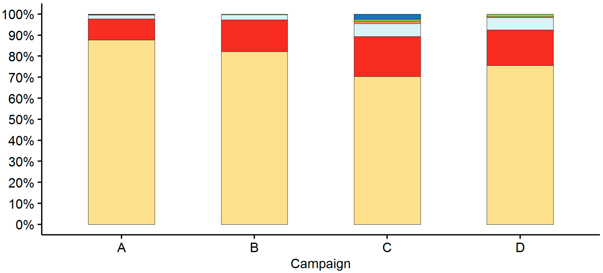
When focusing on machine operation only (SSH_Operation), the productive work time (PSH₀) has, as expected, the highest share of the overall times (Figure 4), as also outlined by a high MU_Operation compared to MU_Total (Table A2). ITs are dominating the SSH_Operation next to the productive work time among all four campaigns. Main cause of IT have been interruptions of the yarding process caused by hang ups but also frequent discussions between the yarder operator and choker setter on the radio, to clarify the work procedures and other work-related issues (

Table A4. Most frequent occurring single delay events during SSH_Operation, their total duration and associated cumulative production deficit in m³ based on unproductive time with reference to PSH₀.

Campaign A				Campaign B				Campaign C				Campaign D
Delay	n	min	deficit (m3)	Delay	n	min	deficit (m3)	Delay	n	min	deficit (m3)	Delay	n	min	deficit (m3)
Discussion on radio	51	21.67	2.09	Hang Ups	43	44.66	4.76	Hang Ups	97	195.11	17.01	Resting	57	20.45	2.17
Carriage repositioning	36	8.66	0.84	Discussion on radio	39	13.9	1.48	Load re-positioning through carriage	93	71.34	6.22	Hang Ups	56	68.22	7.24
Hang Ups	24	48.63	4.69	Resting	23	9.24	0.99	Discussion on radio	70	36.42	3.17	Discussion on radio	33	11.41	1.21
Resting	20	4.49	0.43	Carriage repositioning	14	5.76	0.61	Resting	49	22.26	1.94	Load re-positioning through carriage	29	18.95	2.01
Mainline too tight	16	2.68	0.26	Carriage without pressure	8	9.66	1.03	Mainline too tight	37	16.14	1.41	Adding load	27	39.78	4.22
Stuck choker during unhooking	15	4.06	0.39	Manual positioning of logs	7	4.65	0.50	Slash hindering unhooking	36	18.88	1.65	Carriage without pressure	25	22.61	2.40
Choker not fixed properly	9	10.32	1.00	Mainline too tight	6	1.07	0.11	Stuck choker during unhooking	27	8.86	0.77	Slash hindering unhooking	15	5.88	0.62
Digging out log	8	3.00	0.29	Choker setter on phone	5	1.33	0.14	Carriage repositioning	20	9.26	0.81	Digging out' logs	11	4.60	0.49
Straight spooling of mainline	7	5.28	0.51	Slash hindering unhooking	4	1.59	0.17	Carriage without pressure	18	25.70	2.24	Hook up of chain saw	11	13.43	1.43
Loader blocks landing	7	3.04	0.29	Stuck choker during unhooking	4	1.63	0.17	Waiting for signal	15	5.69	0.50	Delimbing of stem at corridor	11	9.62	1.02

). In contrast to the SSH_Total, PTs only make up a small fraction amongst all campaigns but increased its share within the last two campaigns. They mainly consisted of building up pressure on the carriage as a necessity due to short yarding distances and tensioning of the skyline, which were both frequently occurring but only accounted for short lasting PTs.

Neither on an operational nor on shift level did MT (maintenance time) or RP (rest and personal times) play a major role.

Among the models computed for net-cycle times through stepwise multiple regressions, the campaign B data set model had the lowest fit, which explains only 36% of the observed variance (

Table 5. Stepwise Multiple Regression Models and Test Statistics for the Cycle Times (t_cycle) of the Four Data Collection Campaigns Based on Qualified Observations (n).

${\mathit{t}}_{\mathbf{c}\mathbf{y}\mathbf{c}\mathbf{l}\mathbf{e}}$	Coefficients *	n	R2	F-test		Standard Error	t-test
				F	p		t	p
Campaign A	1.494	170	0.61	50.321	<0.001	0.474	3.154	0.002
	+0.034 *yd					0.003	13.170	<0.001
	+0.075 *ld					0.008	9.894	<0.001
	+0.063 *sl					0.009	7.138	<0.001
	−0.037 *osl					0.005	−6.790	<0.001
	−0.307 *veg					0.114	−2.701	0.008
Campaign B	2.486	81	0.36	10.752	<0.001	0.513	4.843	<0.001
	+0.014 *yd					0.005	2.821	0.006
	+0.045 *ld					0.012	3.696	<0.001
	+0.289 *ln					0.097	2.977	0.004
	+0.916 *vol					0.435	2.109	0.038
Campaign C	2.979	216	0.66	56.658	<0.001	0.450	6.625	<0.001
	+0.050 *ld					0.005	9.693	<0.001
	+0.012 *yd					0.001	13.420	<0.001
	+0.328 *ln					0.061	5.344	<0.001
	−0.051 *sl					0.010	−4.938	<0.001
	+1.150 *vol					0.292	3.933	<0.001
	+0.222 *lp					0.098	2.257	0.025
	0.169 *veg					0.085	1.985	0.049
Campaign D	2.523	159	0.41	35.523	<0.001	0.245	10.280	<0.001
	+0.051 *ld					0.007	7.014	<0.001
	+0.362 *ln					0.050	7.268	<0.001
	+0.010 *yd					0.002	4.252	<0.001

* Notation: yd = yarding distance (m); lp = log presentation (category); ld = lateral distance (m); sl = slope (%); osl = off-set slope (°); veg = vegetation (category); ln = log numbers (n); vol = volume (m³).

). In contrast, the model of best fit explains 66% (Table 5) of the variance and was generated for the campaign C data set. Campaign C had the highest number of observations but also the highest rate of disturbances through IT and PT on the machine operation times (18.9% and 6.1%, respectively) (Figure 4) when compared to the other three campaigns. Although the number of explanatory variables differed between the campaigns, “Yarding Distance” and “Lateral Distance” are included in all models and not surprisingly, have significant effects on net-cycle times.

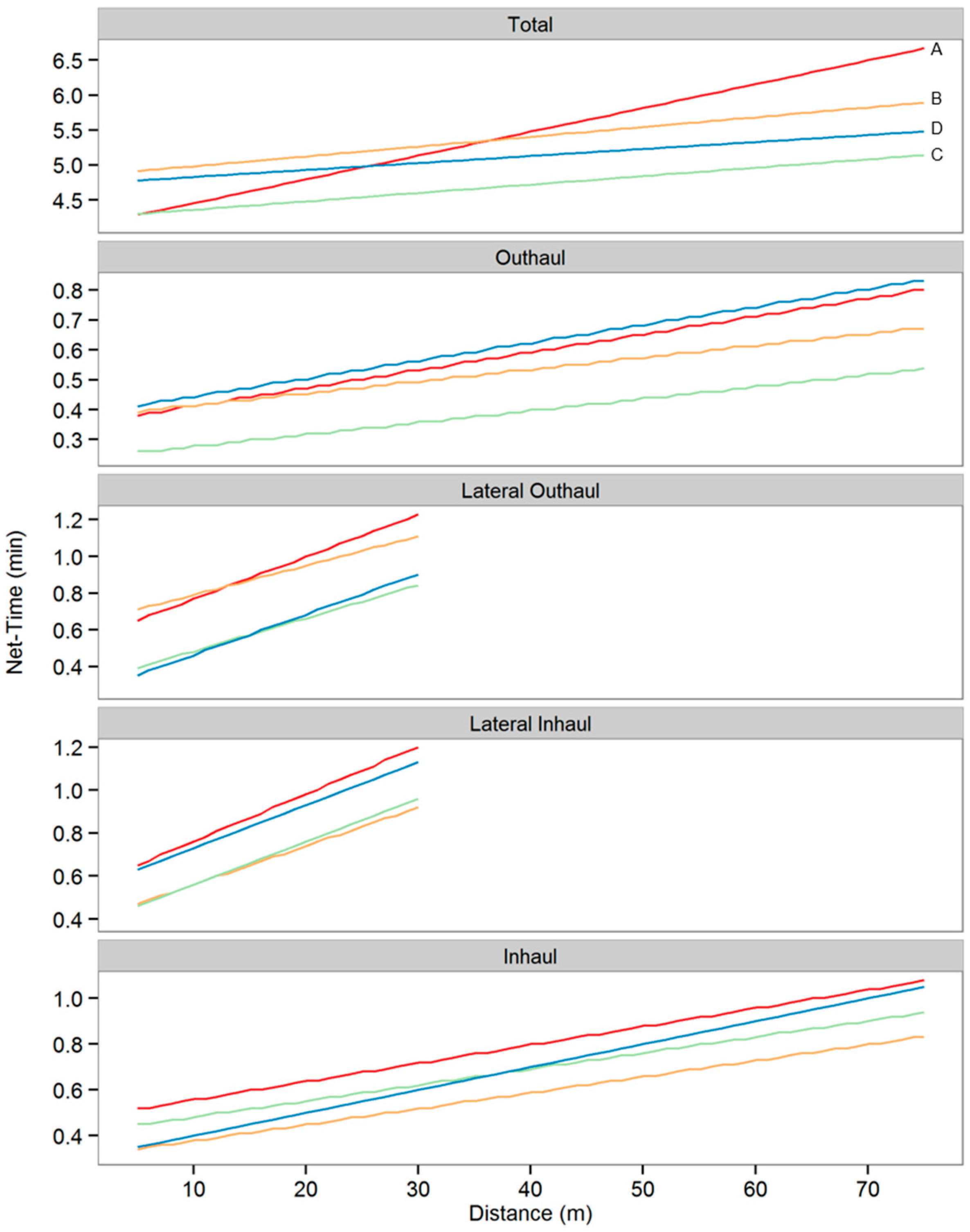
A standardization attempt was undertaken by using the individual cycle time equations (Table 5) of the four campaigns and the overall mean values of all four campaigns (Table 4) for the various independent variables. Under these assumptions, the observations during campaign C again revealed the shortest mean cycle times (5.10 min/cycle), followed by campaign D (5.44 min/cycle), campaign B (5.85 min/cycle) and campaign A (6.55 min/cycle). Plotting the standardized independent variables with the mean values over an increasing yarding distance up to 75 m, a yarding range covered by all studied corridors, gives a general confirmation of these indications (Figure 5). Furthermore, the visualization shows that during the first campaign A, cycle times with associated short yarding distances were relatively short in duration but ascend faster with increasing yarding distances than during the other periods, particularly at ranges above 25 m.

The same approach has been used to illustrate the differences between the individual campaigns for the net Outhaul, Lateral Outhaul, Lateral Inhaul and Inhaul times, using the cycle element’s individual regression models (

Table A5. Stepwise multiple regression models and test statistics for the individual cycle elements of the four data collection campaigns based on qualified observations after removals of extreme values outside three times the standard deviations (n).

Campaign	Element	Coefficients *	n	R2	F-Test		Standard Error	t-Test
					F-Value	p		t-Value	p
A	Outhaul Time	0.369	167	0.62	88.53	<0.001	0.045	8.187	<0.001
		+0.006 *yd					0.000	16.04	<0.001
		−0.004 *osl					0.001	−5.793	<0.001
		+0.002 *sl					0.001	2.274	0.024
	Lateral Outhaul Time	0.454	167	0.33	26.78	<0.001	0.066	6.868	<0.001
		+0.023 *ld					0.003	8.400	<0.001
		+0.003 *yd					0.001	3.995	<0.001
		−0.086 * veg					0.031	−2.756	0.007
	Hook Up Time	1.102	167	0.15	14.76	<0.001	0.144	7.648	<0.001
		+0.294 * lp					0.071	4.139	<0.001
		+0.013 * ld					0.004	3.351	0.001
	Lateral Inhaul Time	0.270	167	0.46	27.843	<0.001	0.151	1.789	0.075
		+0.022 *ld					0.003	8.845	<0.001
		+0.005 *yd					0.001	6.422	<0.001
		−0.009 *osl					0.002	−4.955	<0.001
		−0.101 *veg					0.036	−2.814	0.006
		+0.007 * sl					0.003	2.435	0.016
	Inhaul	0.034	168	0.73	148.70	<0.001	0.054	0.634	0.527
		+0.008 *yd					<0.001	18.821	<0.001
		+0.008 *sl					0.001	7.002	<0.001
		+0.179 *vol					0.062	2.889	0.004
	Unhooking	0.209	168	0.17	16.38	<0.001	0.070	2.972	0.003
		+0.005 *sl					0.001	5.413	<0.001
		+0.030 *ln					0.014	2.165	0.032
B	Outhaul Time	0.373	83	0.28	31.338	<0.001	0.030	12.511	<0.001
		+0.004 * yd					0.001	5.598	<0.001
	Lateral Outhaul Time	0.630	81	0.12	10.779	0.002	0.111	5.685	<0.001
		+0.016 *ld					0.005	3.283	0.002
	Hook Up Time	0.832	81	0.21	21.282	<0.001	0.221	3.761	<0.001
		+0.266 *ln					0.058	4.613	<0.001
	Lateral Inhaul Time	0.379	82	0.29	16.461	<0.001	0.116	3.281	0.002
		+0.018 *ld					0.004	5.115	<0.001
		+0.408 *vol					0.125	3.277	0.002
	Inhaul	−0.389	81	0.74	73.543	<0.001	0.130	−2.991	0.004
		+0.007 *yd					0.001	10.032	<0.001
		+0.328 *vol					0.057	5.768	<0.001
		+0.012 *sl					0.003	4.360	<0.001
	Unhooking	0.544	81	0.14	12.877	0.001	0.048	11.388	<0.001
		+0.259 *ln					0.072	3.588	0.001
C	Outhaul Time	0.577	217	0.88	748.768	<0.001	0.039	14.889	<0.001
		+0.004 *yd					<0.001	36.315	<0.001
		−0.008 *sl					0.001	−7.785	<0.001
	Lateral Outhaul time	0.930	214	0.44	54.681	<0.001	0.150	6.177	<0.001
		+0.018 *ld					0.002	8.238	<0.001
		−0.020 *sl					0.004	−5.288	<0.001
		+0.148 *veg					0.036	4.098	<0.001
	Hook Up Time	0.579	204	0.26	23.263	<0.001	0.143	4.063	<0.001
		+0.162 *ln					0.040	4.095	<0.001
		+0.011 *ld					0.003	3.983	<0.001
		+0.482 *vol					0.159	3.022	0.003
	Lateral Inhaul Time	0.665	216	0.53	78.561	<0.001	0.094	7.110	<0.001
		+0.020 *ld					0.001	14.604	<0.001
		−0.009 *sl					0.003	−3.256	0.001
		+0.163 *vol					0.065	2.515	0.013
	Inhaul Time	0.257	216	0.79	410.052	<0.001	0.062	4.125	<0.001
		+0.007 *yd					<0.001	28.623	<0.001
		+0.043 *ln					0.014	3.026	0.003
	Unhooking Time	0.426	216	0.21	55.289	<0.001	0.043	9.864	<0.001
		+0.089 * ln					0.012	7.436	<0.001
D	Outhaul Time	0.265	158	0.76	165.368	<0.001	0.060	4.413	<0.001
		+0.006 *yd					<0.001	21.069	<0.001
		+0.008 *osl					0.002	4.863	<0.001
		−0.002 *sl					0.001	−2.078	<0.001
	Lateral Outhaul time	−0.207	159	0.38	23.691	<0.001	0.236	−0.877	0.382
		+0.022 *ld					0.003	7.957	<0.001
		+0.013 *sl					0.004	3.390	0.001
		+0.150 *veg					0.047	3.224	0.002
		−0.013 *osl					0.005	−2.507	0.013
	Hook Up Time	1.796	160	0.20	19.413	<0.001	0.386	4.649	<0.001
		+0.215 *ln					0.037	5.862	<0.001
		−0.020 *sl					0.007	−2.799	0.006
	Lateral Inhaul Time	0.387	160	0.40	53.16	<0.001	0.041	9.384	<0.001
		+0.020 *ld					0.002	9.655	<0.001
		+0.002 *yd					0.001	2.564	0.011
	Inhaul Time	0.420	160	0.75	158.960	<0.001	0.106	3.978	<0.001
		+0.010 *yd					<0.001	21.708	<0.001
		+0.163 *vol					0.048	3.387	<0.001
		−0.005 *sl					0.002	−2.583	0.011
	Unhooking Time	0.321	161	0.28	62.341	<0.001	0.036	8.815	<0.001
		+0.084 *ln					0.011	7.896	<0.001

* Notation: yd = yarding distance (m); lp = log presentation (category); ld = lateral distance (m); sl = slope (%); osl = off-set slope (°); veg = vegetation (category); ln = log numbers (n); vol = volume (m³).

) and the time demand dependent on yarding distance (up to 75 m) and lateral distance (up to 30 m) for the associated element (Figure 5).

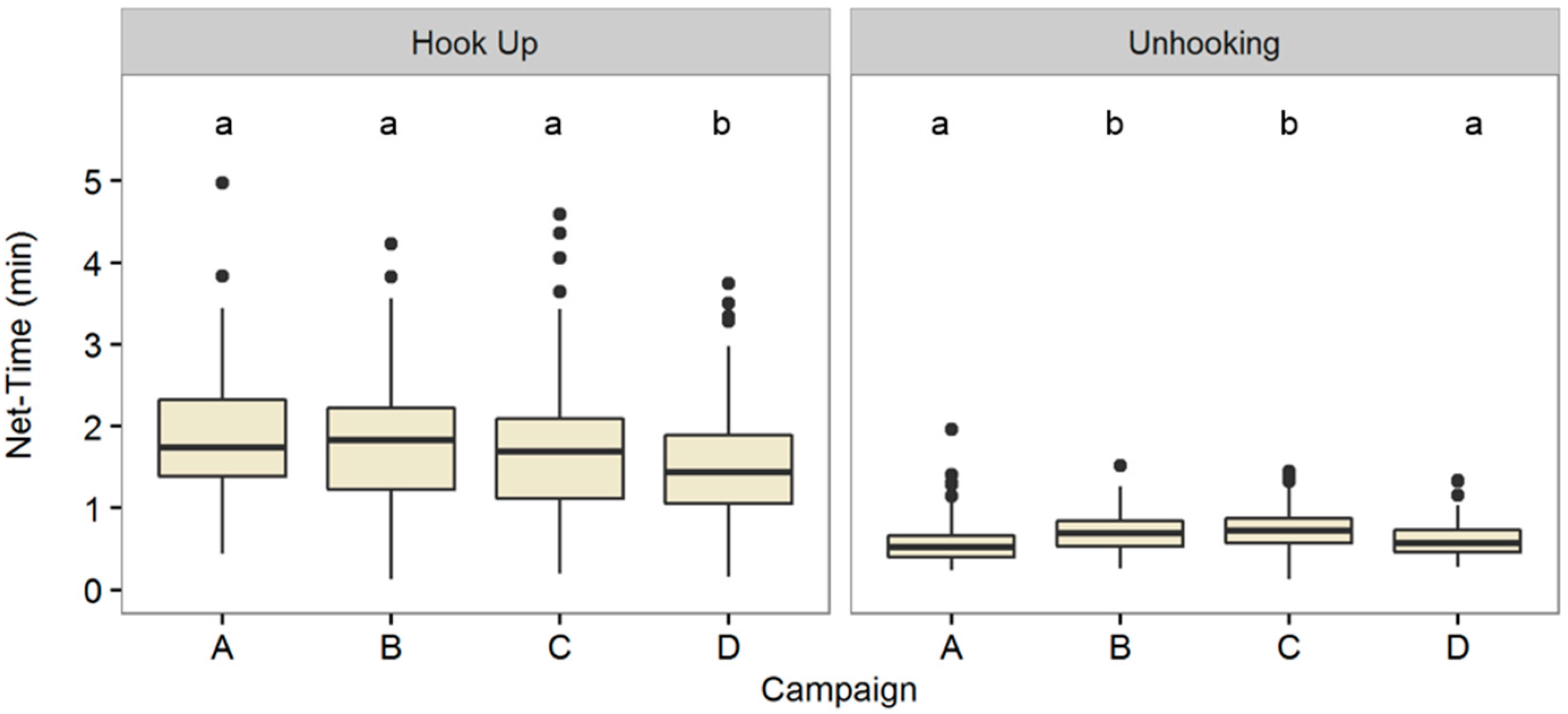
The individual models for Hook Up and Unhooking times (Table A5) have no joint significant predictor that can conveniently display the effects of operational conditions such as yarding or lateral distance for Outhaul and Inhaul and Lateral Outhaul and Lateral Inhaul, respectively. Therefore, box plots (Figure 6) have been used to visualize the variation in time demand between the campaigns of these cycle elements. The median values for Hook Up and 50% of the respective observations show a lower time demand for campaign D, with a significant difference of the mean time (Df = 3, p < 0.05) compared to the previous campaigns. Individual outliers (Figure 6) can generally be associated to poor log presentation with slash or crossed over logs hampering the choker setting, but also due to individual logs located at ridges that were difficult to reach.

The relatively short times for Unhooking compared to Hook Up show higher time demand for campaign B and C and shorter demand for campaign A and D (Figure 6). The difference of campaign A and D were both significant compared to B and C in terms of time demand (Df = 3, p < 0.01). An abrupt increase of mean lateral yarding distances by 33% occurred from campaign A to B, while campaign C had almost similarly long mean lateral distances as campaign B (Table 4). Consequently, a reduced lift effect was observed by the time keepers during the Lateral Inhaul associated to the longer lateral distances. This caused the load to be dragged on the ground through the understory, twisting the chokers, taking up vegetation and slash which impeded the Unhooking and led to delays such as slash hindering the Unhooking process (see Table A4). During the last field campaign in 2015 (campaign D), the lateral yarding distances had again been reduced and this time, the amount of co-extracted slash to the log deck resulted in a lower average time demand for Unhooking when compared to campaigns B and C.

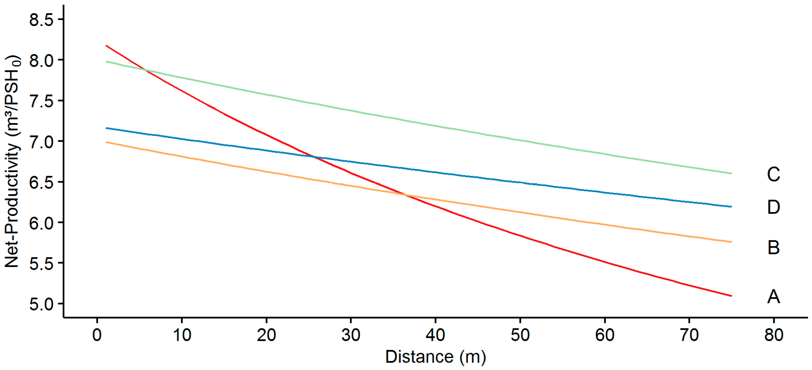
The use of standardized cycle times (as in Figure 5) for calculation of comparative mean net-productivity would generate 6.65 m³/PSH₀ for the most productive operation campaign C, followed by 6.23 m³/PSH₀ for campaign D, 5.81 m³/PSH₀ for campaign B and 5.18 m³/PSH₀ for campaign A. When the net-productivity is displayed for increasing yarding distance of up to 75 m, which was covered within all corridors (Figure 7), it shows relatively consistent parallel trends for campaigns C, D and B, similar to those of the pure cycle times. The productivity during campaign A was very high within the short distances, even superior to campaign C but the performance drops rapidly with increasing distances, being below that of all the other campaigns beyond the 37 m mark.

3.2. Log Book Records

Keeping a log book was a challenge for the cable yarding crew and initial recordings had to be discarded due to incomplete data and false classification of the individual times. After a technical review during field campaign B, useable recordings were achieved for the period from May 2014 to July 2015, covering 32 corridors and 2344 yarding cycles. This period equals 422 days, including 287 potential work days after deduction of weekends and regional holidays. Yet, actual work related to the yarding operation was scheduled and executed only on 197 days, amounting to a total yarded volume of 1392.4 m³, which represents a mean gross daily output of 7.1 m³. Heavy rainfalls impeding forest operations were the main cause of the reduction in work days; access to the forest also continued to be restricted in subsequent days due to poor forest road standards. Additional down days were caused by institutional deficits associated to selection of cut blocks and delays of issuing corresponding harvesting permits. Finally, deficits in timely communication of work progress effected delays in completion of planning and organizing work of subsequent operations.

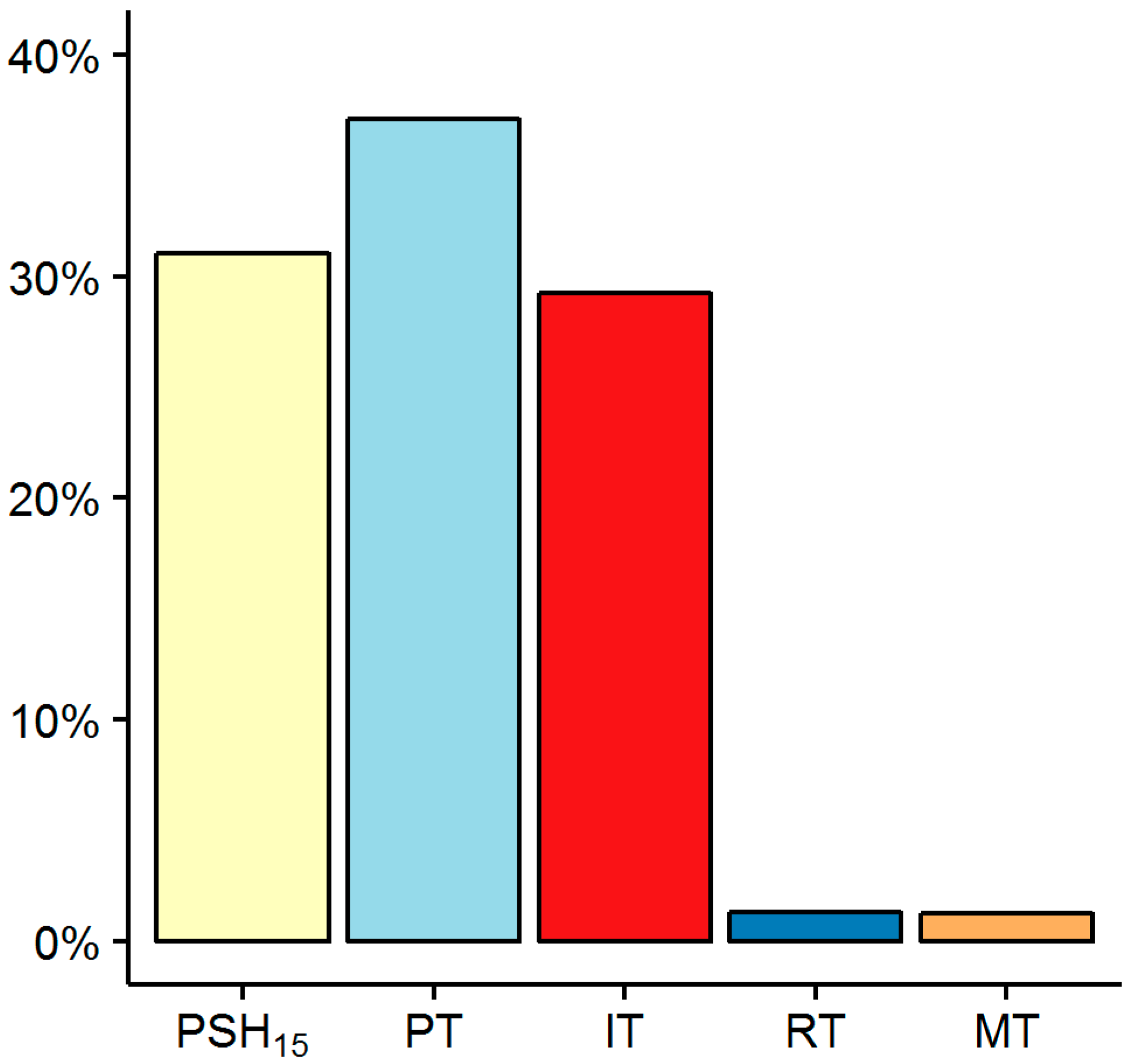
There are 1122.1 SSH that were recorded in total (SSH_Total), which amount to a productive work time of 348.4 PSH₁₅, representing a MU_Total of 31.0%. The high share of PT (37.1%) (Figure 8) is again mainly associated to rigging activities. Recorded rigging times and corridor specifications showed that the average corridor had a length of 113 m, was spaced at 44 m, had one intermediate support, required a total mean set-up time of 5.1 h and corresponding mean take-down time of 2.0 h. This is also covered by the ranges observed in the 12 corridors during the four field campaigns, although these long term average time demands are slightly longer. The share of IT (29.3%) (Figure 8) sums up to a total of 200.4 h, of which 129.8 h were associated to truck loading by the loader. Logistical timing deficits were identified that resulted in the use of the knuckle boom loader, which is obligatory for efficient operation of the yarding system and for truck loading processes instead of clearing the log deck of the yarder; and by this, interrupting the yarder operation leading to avoidable reductions in PSH₁₅. Further cases in which IT reduced the potential MU_Total were: backlogs in tree felling, road construction and leveling of landings. As mentioned before, during the long term monitoring, IT contributed to 29% of the overall SSH_Total, nearly twice as much as the 15% average throughout the detailed time studies. In contrast, over the long-term the dominant time demand for PT, 37.1%, was generally shorter than that of the detailed time studies and made up approximately half of the SSH_Total, apart from campaign B, for which it amounted to 1/5 of SSH_Total (Figure 3). RP times did not occur during the long-term records since short breaks and rests are already included within the PSH₁₅ due to the recordings of lesser detail.

From the log book recordings and calculated SSH_Total system utilization an overall performance estimate was derived. Considering 365 days per year, SSH_Total was generated by deducting weekends and local holidays resulting in 245 potential work days per year. Assuming eight hour daily shifts (working hours without accounting for break times), this sums up to 1960 SSH_Total/year, which relates to 608 PSH₁₅ when considering a 31% MU_Total, as revealed by the log book. Based on the recorded log book performance of approximately 4 m³/PSH₁₅ this results in a theoretical output of 2428 m³/year or 202 m³/month. By considering every potential work day during the studied period, the log book recordings revealed that in practice, a mean value of system employment of only 5.7 SSH_Total/day can be assigned. At the recorded productivity level of the long term records, an extrapolation of these figures on an annual level would result in 1396 SSH_Total, 433 PSH₁₅ and a corresponding total annual productivity expectation of 1732 m³. Machine scheduling and cost estimations should however, actually be based on full working days. Therefore, it is more plausible to account for full work days with eight hour shifts and to apply a reduction factor that is based on the ratio of potential work days and actual observed work days during the long-term recordings, which in this case amounts to 0.59. Under these assumptions, 139 working days remain annually. If proper organization would allow for full eight SSH_Total shifts on each of these work days, the current annual capacity of the crew under local conditions would amount to 1112 SSH_Total hours with an output of 1379 m³ at a 31% MU_Total.

3.3. Efficiency Analysis by Stochastic Frontier Analysis (SFA)

Based on the identified independent variables for the cycle time equations, variables were chosen to define the inefficiency model (Equation (6)) for the technical inefficiency component $u$ in the SFA. Since these variables are significantly affecting the cycle time demand, the input variables for the production function, Equation (4) but are not directly related to the skill level of the crew, they are a source of inefficiency affecting the crews’ EEF and thus can be accounted for by the SFA model (Equation (5)). This implies that the remaining deviation from the potential frontier isoquant can be related to the skill and performance level of the crew.

$$u=z_0+z_1\text{yd}+z_2\text{ld}+z_3{\text{veg}}_{\text{in}}+z_4{\text{lp}}_{\text{in}}+z_5{\text{sl}}_{\text{in}}$$

(6)

where:

• u = is the nonnegative technical inefficiency component
• z = is a parameter to be estimated
• yd = is the yarding distance (m)
• ld = is the lateral distance (m)
• veg_in = is the indicator for vegetation hindrance (yes/no)
• lp_in = is the indicator for the quality of log presentation (bad/good)
• sl_in = is the indicator for terrain slope (>35%: yes/no)

The data originally collected for the 3-level factor variables $\text{veg}$ and $\text{lp}$, as well as the numeric variable $\text{sl}$, were converted into binary (indicator) variables in order to simplify the inefficiency model. Where ${\text{veg}}_{\text{in}}$ and ${\text{lp}}_{\text{in}}$ indicates an effect above the original level 1 and ${\text{sl}}_{\text{in}}$ considers the terrain to be steep above a gradient of 35%. Values “yes” and “bad” were used in the model as a dummy variable 1; otherwise 0 was used.

The SFA is summarized in

Table 6. Maximum Likelihood Estimates of the Parameters of the Stochastic Frontier Analysis.

Parameter	Coefficient	Standard Error	Z Value	Pr (>|z|)
Stochastic Production Function
Intercept, ${\mathsf{\beta }}_0$	−1.13	0.125	−9.04	<0.001
ln (Cycle Time, T), $\mathsf{\beta }1$	0.24	0.077	3.08	0.002
ln (Number of Logs, L), $\mathsf{\beta }2$	0.48	0.046	10.45	<0.001
Inefficiency Model
Intercept, $z_0$	0.365	0.194	1.88	0.060
Yarding Distance, $z_{1}yd$	0.001	0.001	1.68	0.092
Lateral Distance, $z_{2}ld$	0.005	0.004	1.40	0.161
Vegetation, $z_3{\text{veg}}_{\text{in}}$	−0.027	0.090	−0.29	0.768
Log Presentation, $z_4{\text{lp}}_{\text{in}}$	0.150	0.087	1.74	0.083
Slope, ${\mathrm{z}}_5{\text{sl}}_{\text{in}}$	−0.439	0.108	−4.06	<0.001
${\mathsf{\sigma }}^2$	0.30	0.060	5.03	<0.001
$\mathsf{\gamma }$	0.86	0.387	22.24	<0.001
Log-Likelihood Value	−349.80

with the corresponding maximum likelihood estimates of the stochastic frontier production function (Equation (5)) and the inefficiency model (Equation (6)).

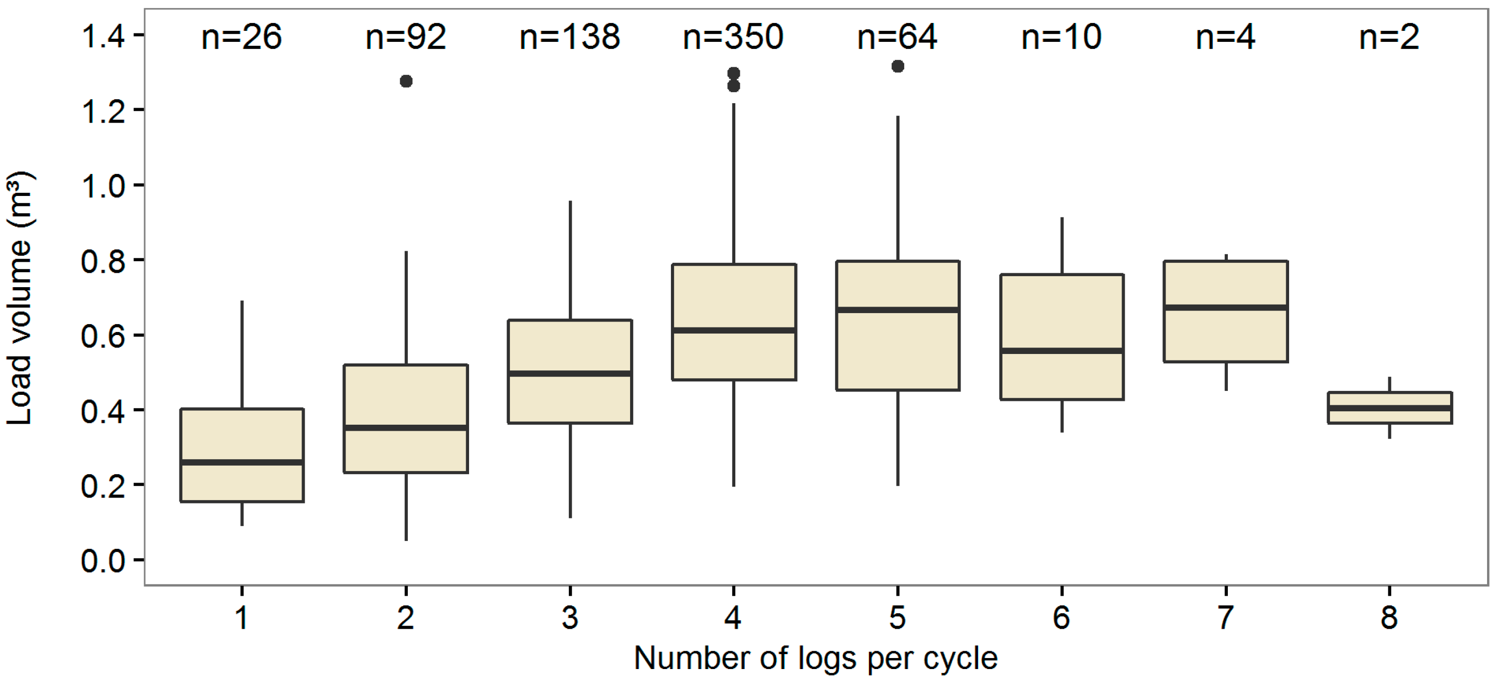
The two variables of the production function, namely cycle time (T) and number of logs (L), have positive and highly significant coefficients, confirming their high contribution to output productivity in volume per turn. The elasticity of the coefficients assign at a cycle time increase by 1% an increase of the production output by 0.24% and an increase in number of logs by 1%, would increase the production output by 0.48%. The returns of scale, as the sum of the input coefficients is <1, affirming the production function having decreasing returns to scale. The scale effect (coefficient) of the number of logs on productivity (output) is higher compared to that of the cycle time. However, the piece size is also a highly influential factor when considering cycle output with the load volume in relation to the number of logs per cycle. It is obvious that if the log number exceeds the amount of the four available chokers, then the individual piece size generally decreases once more, since only smaller logs are choked together by one choker cable. This results in decreasing load volumes, particularly when eight logs are attached, although observed only twice (Figure 9).

Among the variables determined for the inefficiency model, only slope showed a significant effect on efficiency (Table 6), with the negative coefficient indicating that steeper slopes would decrease the inefficiency. The coefficient for $\mathsf{\gamma }$ indicates that approximately 86% of the deviation from the ideal production is explained by technical inefficiency (u) and that the noise (v) is of minor influence. A likelihood ratio test as integral part of the package frontier [32], was conducted in order to verify whether the inefficiency term u significantly improves the fit of the frontier model by comparing the stochastic frontier model with the corresponding OLS model under the hypothesis H₀: γ = 0 (

Table 7. Likelihood Ratio Test of the SFA Model with the Degrees of Freedom (Df), Log Likelihood Values (LogLik) and Test Statistics for the Assumed χ²-Distribution [27].

Model	Df	LogLik	Df	χ2	Pr (>χ2)
Model 1: OLS (no inefficiency)	4	−397.15
Model 2: Efficiency Effects Frontier (EEF)	11	−349.80	7	94.704	<0.001

). As H₀ is rejected, the presence of technical inefficiency is furthermore confirmed and a justification of the stochastic frontier model with the EEF established.

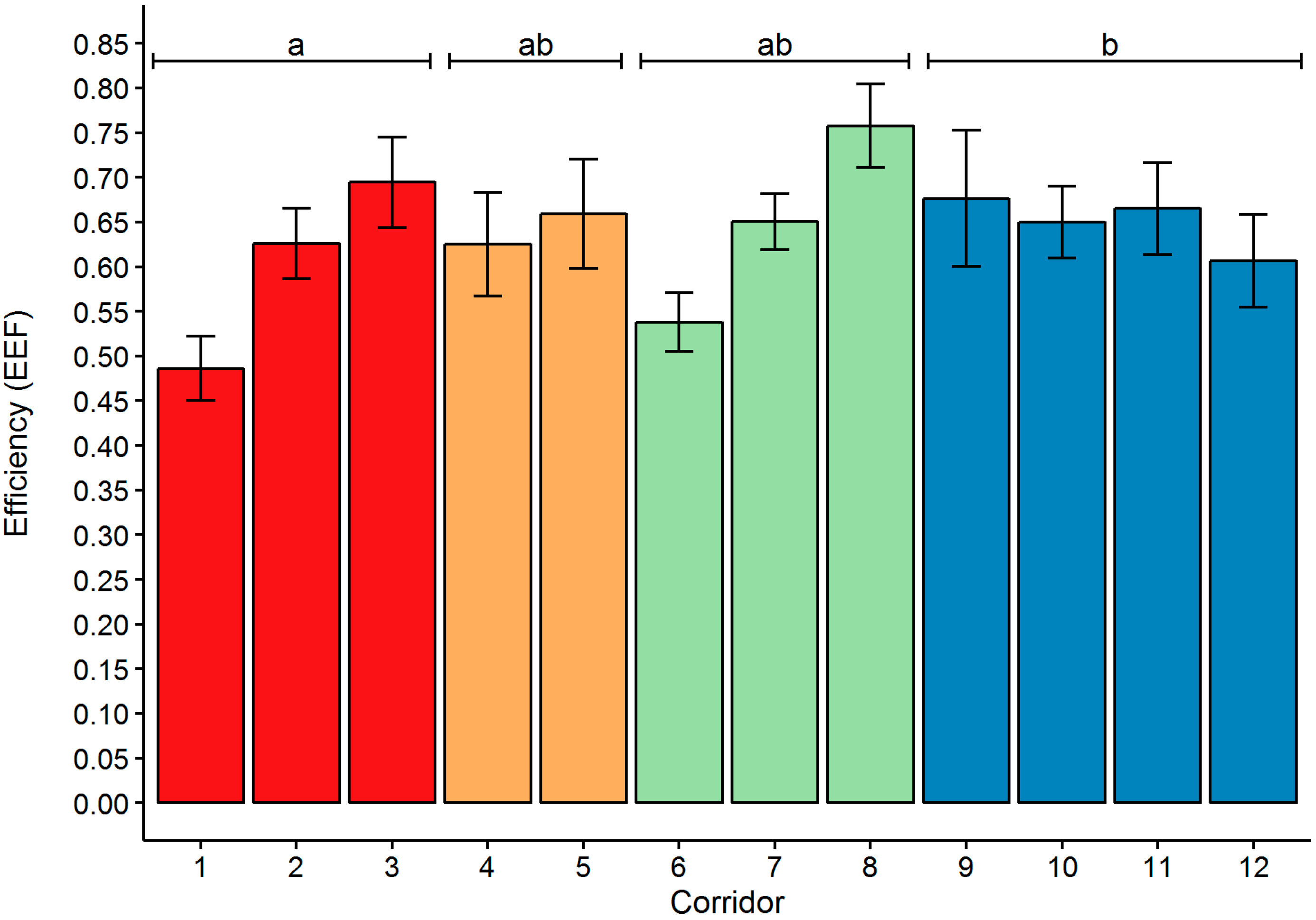
The mean efficiency of the crew for all assessed yarding cycles during the period monitored was determined to have an EEF value of 0.62, representing 62% of the potential achievable output at the given input resources. The efficiency levels within the yarding cycles ranged from 0.18 to 0.95, showing variability across the entire period with no pattern, indicating a steady learning process, and the crew not having achieved a working routine yet. Grouping the mean efficiency values of assessed yarding cycles for each individual corridor and according to time periods associated the four field campaigns (Figure 10), it is noticeable that at every campaign, the crew usually began with a low mean efficiency but improved by the next corridor within the same campaign. The overall lowest mean efficiency of 0.59 was encountered during campaign A and it also included the lowest mean efficiency at corridor level of 0.49 for corridor 1, directly at the beginning of the entire campaign. A significant difference between the mean efficiency values of corridor 1 and 2 is indicated by the confidence intervals (95%) that do not overlap which was in contrast to corridor 2 and 3, which had different means but overlapping confidence intervals. In addition, the confidence intervals of the corridors of the following period, campaign B, do not show significant differences in their mean efficiency, neither within the campaign nor to the previous one. Campaign C, however, shows a significantly lower mean efficiency value for its first corridor (corridor 6), compared to the previous campaign but a significant improvement for every additional corridor of the period. Although small fluctuations are visible in campaign D, the mean efficiency values do not differ significantly among all the corridors, which leads to a high mean efficiency value of 0.65, the highest among all campaigns. The efficiency is relative consistent within campaign D and shows no significant difference between the first corridor of campaign D and the last one of campaign C. This could indicate a certain degree of performance stabilization and with an approach towards the learning plateau, also indicated by a significant difference (Kruskal Wallis test; Df = 3, p = 0.02) between the overall mean efficiency value for campaign A (0.59) and campaign D (0.65) (Figure 10).

4. Discussion

The objective of this study was to analyze and evaluate the performance level and its change over time of a professionally trained, start-up cable yarding crew in China. This was conducted while applying a combination of methodologies to determine indicators for performance assessment and enhancement and to evaluate the overall suitability of standing skyline systems in meeting local demands under changing forest management schemes.

The effect of a crew’s experience level within a production system refers to the learning theory and description of the learning curve [34]. Improvements in work efficiency are achieved through the repetition of a specific work task until the curve flattens, determining the learning plateau and approving the skill level of an experienced professional [35]. The theory of learning and its related effect on productivity has its origin in the manufacturing industry, which is characterized by identical work objects and rather constant work environments and conditions. The complex work environment in forestry does not compare to this, with its numerous influencing variables of which not all can be accounted for [36], especially in cable yarding operations [37]. Hence, the application of learning curve models in forestry and its adaptation to harvesting systems has either been conducted through controlled, simulated conditions (e.g., [38]) or with less variable harvesting systems in homogenous stands, such as fully mechanized harvesting in intensively managed conifer stands (e.g., [39]). Although previous attempts have been made to demonstrate learning effects for cable yarding crews through in-field productivity studies, the time frames for monitoring were either rather short if conducted on detailed level (e.g., [40]), or they only included operator summaries, limiting the overall relevance of the results (e.g., [41]). Previous attempts mostly used approved and accepted methodologies of work and time studies, each with its advantages and disadvantages (see [19]). This study combined various methodologies in order to overcome uncertainties experienced in earlier studies. One constraint however, is that it only represents one crew and thus bears the limitations associated with the individual behaviors of this crew and their experience of site specific operating conditions, with this adding a “case study” character to the research. Nevertheless, the results still offer indications regarding the performance and potentially influencing factors that are typical for the local situation in southern China.

4.1. Performance and Skill Development

Generally, the studied crew showed that they were able to work with the yarder system in a productive way without any additional external support after completing a basic training, which only lasted for two weeks. With respect to the extracted log dimensions and associated log volumes of in average 0.16 m³, the crew was able to overcome the physical limitations of conventional manual wood extraction systems which are limited to log volumes of approximately 0.04 m³ (see [6]). The crew also demonstrated the yarding system’s technical feasibility for implementing new silvicultural objectives (e.g., [3]) by thinning operations without major damages to the remaining stand.

The most significant independent variables for the total extraction cycle time demand were yarding distance, lateral distance and also the number of logs; this is in line with other cable yarding studies (e.g., [8,42,43,44]).

The comparison of the productivity results of the first time study data set of 2013 (campaign A) with other published figures for the same yarder (e.g., [45]), shows comparable values when considering the differences in area size and extraction conditions. This is remarkable given that the 2013 study was conducted directly after the initial training, while the crew had only limited experience. It confirms a quick skill development process in an initial learning phase, after overcoming the beginners’ stadium and is represented by a typical learning curve of sigmoid shape (e.g., [39]). However, comparing the productivity values of the first time study with the subsequent ones, under consideration of the different yarding distances, only minor improvements can be seen in the standardized cycle time and output levels, with the last time study in 2015 even showing a slight decrease in mean performance.

Extending the analysis by including log book recordings revealed large breaks between consecutive operating days, lasting from a few days up to as much as three months. Reasons for the breaks were associated to organizational and institutional problems but also local precipitation pattern and the ensuing inaccessibility of the plantations, due to the low forest road standard. Although a linear improvement in productivity is projected by the learning curve theory [35], periodic interruptions of operations with longer down times are known to interfere with the learning process and the development of routines. The productivity loss associated to longer production breaks is described by Jaber and Bonney [46] as the Forgetting Phenomenon, which is the degree of forgetting as a function of break length and the level of experience gained prior to the break. The occurrence of forgetting is especially critical in the learning phase of an operating crew, where professional training and associated investments were part of the work system’s and equipment’s introduction and unnecessarily prolongs the skill development phase. Haynes and Visser [40] showed that expenses for professional training can be redeemed within a short period of time due to the gained improvement in productivity and decreasing operating costs. However, longer production breaks, particularly when directly after a training period, hinder practice and retention rates of improved knowledge and skills and impede the reach of training objectives.

Apart from productivity, the performance of the crew was evaluated by means of stochastic frontier analysis (SFA) in order to quantify the efficient use of given inputs to generate a maximum attainable output, as defined by technical efficiency [27], which indicates maximum achievable productivity. The SFA coefficients cycle time (T) and number of logs (L) were both positive and significant (Table 6) and therefore, follow the theory of production in achieving increased output with increased input rates [30]. The crew however worked with a mean efficiency of only 62% (EEF value of 0.62) at the given working conditions, suggesting a general performance improvement potential of 38%. Although different in study design and objectives, these values can be restrictively compared with the findings of the SFA cable yarding study conducted by Aalmo and Baardsen [29]. There, the professional yarding crews in Norway reached mean efficiency values of 88%, with a heavily skewed frequency distribution towards 100% efficiency. In contrast, the evaluated Chinese crew showed a more scattered frequency distribution of the efficiency values, which apart from the generally lower mean efficiency, also indicates inconsistency in performance related to the lack of routine of a skilled work crew.

Fluctuations in the efficiency values between the detailed time study campaigns can obviously be associated to the production breaks and periods of low activity and would refer back to the Forgetting Phenomena [46]. The log book recordings revealed that major efforts were made by the crew to operate the cable yarder for a maximum number of hours during the periods in which the foreign researchers were present, resulting in relatively high daily SSH_Total when compared to the annual average. Furthermore, the share of PT (preparatory time) during the four time study campaigns is relatively low compared to those of the long term records, which underlines the assumption that additional efforts were pursued by management, including more intensive supervision of work execution to prepare in advance for sound operations during the field campaigns. This can be seen as a bias of detailed time studies in general and is a phenomena well described in literature [19]. Generally, this might lead to a certain overestimation of annual SSH_Total and MU_Total based on the study and should be further considered for the figures presented. However, the training effect through consecutive high repetitions became obvious in campaign C, where after a longer production break (five weeks) the crew which began with a low mean efficiency rate at corridor 6, quickly improved and even led to the highest mean efficiency values achieved at corridor 8 at the end of this campaign (Figure 10). Although not particularly evident, these periodic differences can be observed in the first two campaigns as well. The crew always began with low mean efficiency values and improved with the next corridor, confirming the learning and performance improvements by consecutive repetition [35]. Taking into account that campaign C lasted for more than two weeks, it is not surprising that it also showed the highest efficiency improvement amongst the four campaigns. This underlines the need for continuous operations during the start-up phase to ensure quick skill development for higher performance, since it is the phase of most intensive learning [47].

However, this effect is not visible during the last field campaign in 2015 (campaign D), where the crew began on a relatively high mean efficiency level and maintained the performance until the last measured corridor. Here, although not significant, a reduction in mean efficiency was visible (Figure 10). Pre-conditions for campaign D have been similar to campaign B, with a longer production break of three weeks due to holidays, between campaigns C and D. However, the break was shorter than that between campaign B and C (five weeks) and the crew had already worked together for a year and a half. Experience and routine would ensure a quick re-entry in previous performance levels [48], which means they would not necessarily begin at a very low value and would explain the generally higher efficiency values. An explanation for the mean efficiency values of campaign D below the peak of campaign C may be given due to more difficult working conditions because of high temperatures. Outside temperature constitutes an independent variable which was not accounted for in this study. But during campaign D the weather was very hot, with mid-day temperatures above 30 °C accompanied by humidity, which is believed to have reduced the overall performance. High temperatures exponentially decrease the productivity in physical demanding forest operations [49]. In contrast, the drop in mean efficiency on the last measured corridor was most likely related to the replacement of one of the experienced choker setters by an untrained worker.

4.2. Human Resource

One of the originally professional trained choker setters resigned shortly before the end of campaign D, due to unsatisfactory pay. This underlines the importance of binding professionally trained workers through reasonable base salaries complimented by performance based incentives and offering personal career perspectives [50,51]. The human resource is one of the key capitals of a contractor utilizing advanced technology [52]. Particularly in cable yarding operations, it is the seemingly simple task of the choker setter that can be very decisive in determining the efficiency of the operations [37]. Garland [53] also refers to the Hook Up process as being the most critical one in terms of general time duration and delays caused by wrong choker settings—this is confirmed in the present study and other yarding studies (e.g., [54]). However, the Hook Up process is likely dependent on numerous external factors, not all captured in this study. Yet, high efficiency levels can only be achieved by qualified, trained and experienced personnel [37]. Therefore, management should make it a priority to engage well-performing, professional crew members in order to ensure capital intensive equipment is efficiently and safely operated [39]. This could become one of the major challenges for Chinese entrepreneurs when considering both: the 5% predicted annual increase of wages in the Chinese forestry sector, as well as a general reduction of a qualified workforce in rural primary production due to migration to industrial urban centers [1,55].

Despite a crew’s skill level, operating conditions also contribute to the inefficiency of a work crew (e.g., [41]). Within the SFA, the integrated inefficiency model evaluates the effect of selected variables on the efficiency of the crew and accounts for them through the inefficiency term$u$. In this case, however, the inefficiency model only determined slope as a significant source affecting the crew’s productivity (Table 6). Its negative coefficient determines a reduction of inefficiency at increasing slope. This is related to increased speed of the carriage during Outhaul within the applied gravity mode in steep terrain. The individual cycle element models for Outhaul during campaign C and D (Table A5) also indicate a negative, highly significant (p < 0.001) coefficient for slope, implying reduced time demand with increasing slope. The same effect did not occur during the campaigns A and B. This was because the operator did not Outhaul in a gravity mode during campaign A; due to his limited experience with the equipment, he instead used the winch drive to control the carriage travel, which led to a generally lower velocity of the carriage during Outhaul. During campaign B, the corridors were very short, which could have limited the effect of gravity on the Outhaul phase. However, considering the high contribution of the Lateral Outhaul, Hook Up and Lateral Inhaul phases on the total cycle times throughout all campaigns (Table A1), it does not seem plausible that increased slope reduces inefficiency and would correspondingly increase productivity. The mentioned work phases are highly dependent on the mobility of the choker setter and his strength, but slope puts an additional stress on the worker during this already intense work phase [56]. The stress is further intensified with increasing lateral distances, particularly when carrying the cable and chokers [42]. It would thus be misleading to state that slope always positively affected efficiency during campaign C, the campaign with the longest lateral distances. Subsequently, it is also rather unexpected that lateral distance should be a non-significant coefficient in the inefficiency model. Hence, the inefficiency model bears uncertainties that may be linked to the limited number of observations, the variable definition or unaccounted for additional noise in the data, which limits its relevancy within the current study layout.

4.3. System Adaptations

In order to improve the productivity of the crew, the identification of appropriate methodologies to analyze individual skill levels and causes for inefficiency are not the only necessities. It is equally important to look into further technical and organizational adaptions of the system to improve the overall performance under Chinese forest operating conditions.

Radio controlled chokers can increase the productivity and further elevate the automatization of operations and have therefore gained increasing popularity among European cable yarding entrepreneurs [57]. However, European state of the art yarding systems designed for high volume operations, already have a high degree of automatization and the integrated processing units are controlled from a single machine cab or even remotely by radio. Stampfer et al. [57] concluded in their study on the utilization of radio controlled chokers with a cab controlled yarder-processor unit, that a time reduction occurred mainly during the Unhooking process but not during the Hook Up. Our time study results showed that particularly the Hook Up process bears potentials for time improvements due to its high share on the total cycle time, which was on average of 29% over the four campaigns. In contrast, the Unhooking accounted for only 11% of the time, on average. The operator of the K303 H is standing directly next to the log deck and is able to easily release the chokers as long as the log deck is consistently cleared by the loader. Therefore, the Hook Up phase should be the focus of improvement for the investigated system configuration, for instance by a second set of conventional chokers for pre-setting during the carriage travel time. Such an approach has reduced Hook Up times within South-African cable yarding operations, significantly contributing to productivity increments [58]. A second set of chokers might also help to generate optimal load sizes per turn in order to increase productivity, an often underestimated improvement potential [43]. During the studied operations, mean load volumes did not exceed 0.6 m³. Assuming a green density of 1000 kg/m³ for pine logs [59] and fully suspended loads, only approximately 40% of the yarder’s maximum payload capacity of 1.5 t was utilized. Despite the increase in the availability of chokers, good log presentation and pre-bunching for optimal load parcels per turn are additionally important in order to make full use of the technical capacities of the equipment and to increase productivity [54].

Adapting the investigated yarding system to include a second set of chokers would not only suit its technical operation requirements but would also avoid high initial investments and the demanding maintenance associated with the radio controlled chokers [57]. A major downfall of using a second choker set would however, be the reduction in short breaks between the work cycles, which are currently used as a recovery period from the physiological stress experienced by the choker setters during their demanding tasks; this might decrease performance due to work related fatigue [56,60]. Working periods during hot weather cause a likely reduction in performance or the need for more frequent and extended rest and personal times [61]. Regardless of the adaptation, the generally low performance of the crew during the hot period in 2015 (campaign D), indicates that this aspect should be considered in further investigations.

4.4. Work Organization and Planning

In order to compensate for the loss of operating times due to seasonal precipitation peaks, it is often suggested to increase daily SSH_Total during the dry season in order to keep annual SSH_Total at a reasonable level. In this context however, a study by Pasicott and Murphy [62] should be noted: they demonstrated in Chilean forest operations that increasing daily shift times did not necessarily increase productivity in a linear matter. This consideration is particularly important for the Guangxi region since the dry periods are usually combined with high temperatures.

Generally, an increase of PSH₀ over SSH_Operation during an operation is essential in order to increase overall productivity. Therefore, the delays in form of IT (interference time), which are less related to the crew’s skill level but more to organizational and planning tasks, should be reviewed and optimization strategies identified. Hang ups caused major delays during all time study campaigns (Table A4), which often resulted from decreased lift effects of the load during Lateral Inhaul due to extended lateral distances [63]. Another reason for delays was an insufficient quality of log presentation with respect to felling direction, delimbing, crown topping and the slash disturbance, all of which also further negatively affecting Hook Up times [40,58,64]. The subjectively assessed quality of log presentation by the felling crew, which was disconnected from the yarding crew and not covered by this research, was rated throughout the time study campaigns on average only with “fair”. Improvements in log presentation to increase productivity through eased Hook Up by pre-bunched loads can be achieved e.g., through the utilization of single grip harvesters [54]. Due to technical progress (tethering) these harvesters are capable to be utilized in steep terrain cable yarding operations, which is also considered an advancement in work safety [65]. However, currently, cable yarding operations in Guangxi seem to be low volume operations with small cut blocks and low annual SSH_Total, considering the monitored operations as representative for the entire province. The high initial investment costs but also corresponding operation, relocation and maintenance costs associated to harvesters would make it difficult to be cost efficient [66,67]. Additionally, local service infrastructure and professional harvester operators are, to our knowledge, currently only available to a single large-scale foreign operated pulp and paper company in the coastal region of Guangxi. Instead introducing state of the art steep terrain harvesters, another way of increasing productivity of cable yarder operations is by focusing on an integrated training approach of local chainsaw operators. Making them aware of the specific needs of yarding operations and constant communications between the two groups of workers of the forest-wood-supply chain is essential. Furthermore, distinct written work orders and post operation checks of the output by management, including awards of best practice incentives, are means of increasing work quality and long-term performance. Such an approach could increase the yarder’s productivity at much lower costs when compared to the introduction of most likely underutilized, state of the art, steep terrain harvesters. In that context, on the job vocational training approaches derived from identified improvement needs can help to build up a professional, well performing workforce [68].

Certainly at the current level of operations, a priority focus should be given to organizational and administrative improvements. This can noticeably increase MU_Total during the SSH_Total and keep operational delays associated to operation management at a minimum, in order to generally increase operational performance [58]. The observed MU_Total during the field campaigns only ranged from 30.1% to 43.9% and the log book recordings exposed also a low mean MU_Total of only 31%, compared to for example, 66% for cable yarders from long-term records in Austrian operations [69].

Well conducted pre-harvest planning, harvest layout and truck scheduling plays a fundamental role for achieving high productivity and a high MU_Total of a cable yarding operation [40]. Although this is partly the task of higher administrative levels, the on-site operation manager also contributes (through the execution of the scheduled machine operation and floating, the trucking as well as the operation associated supplementary works), to the share of productive work time. The operation manager will also play a fundamental role in corridor layout planning and coordination of rigging activities. While rigging is shown to be one of the major contributors to PT, layout planning of corridors also effects productive times by directly influencing corridor spacing and related lateral yarding distance. Since it was shown in this and previous studies (e.g., [8,58]) that lateral distance has a significant effect on mean cycle time and that increasing lateral distances foster delays such as hang ups and physical stress to choker setters during the Lateral Outhaul, it is important to determine suitable corridor spacing for efficient operations. The limited number of rigging procedures timed in detail during this study did not allow for evaluating the potential benefits of wider corridor spacing, with respect to lower required overall rigging times (due to fewer corridor changes) versus its negative impact on yarding productivity caused by longer lateral distances. Particularly, the relatively low volumes extracted per corridor would indeed favor wider spacing but would also contradict the management aim of a low impact harvesting system, as wider corridors generally bear higher risks of damage to residual trees due to less controlled load movements and lacking suspension (e.g., [70]).

Generally, for very short corridors of less than 50 m in moderate terrain combined with low volume thinning operations, the application of skidders instead of cable yarders should be considered too, as already applied in other regions of China (see [71]). Therefore, further investigations should also focus in more detail on optimal corridor layout and rigging procedures and appropriate system alternatives.

5. Conclusions

This study analyzed how efficient a start-up cable yarding crew in southern China performs over a development phase considering new forest management practices, operating conditions and a changing socio-economic situation. The applied methodologies of operational research and performance evaluation reaffirmed their relevance in the discussion of challenges and socioeconomic environment, such as availability of qualified personnel and operations of scale, not only for the introduction but also the justification of harvesting systems with a higher degree of mechanization. In addition, the combination of traditional time study methods with log book recordings and in forestry so far, rarely used stochastic frontier analysis (SFA), allowed for comprehensive data interpretation. In conclusion, cable yarding is generally considered to be a very complex and sophisticated extraction system with special user requirements. Compared to ground based skidding, it creates challenges in terms of technical operation and accident prevention to the operating crew but also to the planning personnel in order to efficiently utilize such capital intensive equipment. However, the investigated start-up cable yarding crew demonstrated that without having major previous experience in forest operations, they were able to operate the system within a relatively short period after two weeks of professional training. But when considering the high costs and technical capabilities of the equipment, it should be noted that even at the end of the initial monitoring phase of two years, only relatively low system productivities were achieved, which revealed an underutilization of the system’s capacity. In addition, the analysis revealed that the operation performance is not only dependent on a professional and skilled crew. A well organized, high level management is required for work scheduling and operation preparation, as well as the institutional framework and consideration of local climate patterns, also essential in order to ensure productive operations at high annual utilization rates. What is also required is capacity building among all participants of the forest-wood-supply chain, including the fostering of systems-thinking to enhance awareness of interdependency of processes and required contributions of each individual and his effect on total operation efficiency. Such an approach must cover all supply chain levels—ranging from the planning to execution of tree felling, yarding, truck loading and haulage—in order to ensure sustainable commercial forestry operations with technology as a key component. Furthermore, the setting and enforcing of quality standards, including occupational health and safety as well as product quality, but also stand and ground disturbances, should be combined with fair salaries accounting for excellent work. These are prerequisites for enabling successful multiple use forestry as intended by the Chinese government.

References

1. He, H.; Xu, J. Projection of Timber Supply and Demand Trends in China Based on an Econometric Model. For. Prod. J. 2011, 61, 543–551. [Google Scholar] [CrossRef]
2. Wang, G.; Innes, J.L.; Lei, J.; Dai, S.; Wu, S.W. China’s Forestry Reforms. Science 2007, 318, 1556–1557. [Google Scholar] [CrossRef] [PubMed]
3. Liu, S.; Wu, S.; Wang, H. Managing planted forests for multiple uses under a changing environment in China. N. Z. J. For. Sci. 2014, 44, S3. [Google Scholar] [CrossRef]
4. Barr, C.; Cossalter, C. China’s development of a plantation-based wood pulp industry: Government policies, financial incentives, and investment trends. Int. For. Res. 2004, 6, 267–281. [Google Scholar]
5. Nutto, L. Die Eukalyptus-Plantagenwirtschaft in Brasilien. Nachhaltige Holzproduktion oder ökologisches Desaster? Wald Holz 2007, 88, 49–53. [Google Scholar]
6. Engler, B. Gestaltung von Arbeitsprozessen bei der Bewirtschaftung von Eukalyptusplantagen in Süd-China: Analyse gegenwärtiger Arbeitsverfahren und Modellierung eines höheren Mechanisierungsgrades in der Holzernte zur Beurteilung der ökonomischen Auswirkungen. Ph.D. Thesis, Albert-Ludwigs Universität, Freiburg, Germany, 2011. [Google Scholar]
7. Yin, R. Forestry and the environment in China: The current situation and strategic choices. World Dev. 1998, 26, 2153–2167. [Google Scholar] [CrossRef]
8. Huyler, N.K.; LeDoux, C.B. Cycle-Time Equations for the Koller K300 Cable Yarder Operating on Steep Slopes in the Northeast; Research paper; United States Department of Agriculture, Northeastern Forest Experiment Station: Radnor, PA, USA, 1997.
9. Sessions, J. Harvesting Operations in the Tropics; Springer: Berlin, Germany; London, UK, 2007. [Google Scholar]
10. Hoffmann, S.; Jaeger, D.; Schoenherr, S.; Talbot, B. Challenges in Mechanization Efforts of Small Diameter Eucalyptus Harvesting Operations with a Low Capacity Running Skyline Yarder in Southern China. Forests 2015, 6, 2959–2981. [Google Scholar] [CrossRef]
11. Climate-Data.org. Klima: Pingxiang. Available online: http://de.climate-data.org/location/2516/ (accessed on 17 February 2016).
12. Li, J.; Chen, S. Empirical Analysis on the Practical Feasibility of Timber Legality Verification Work in China. Open J. Political Sci. 2015, 05, 167–179. [Google Scholar] [CrossRef]
13. Erler, J.; Grüll, M.; Wächter, M. Bodenschonende Holzernte; Technikmanagement in der Forstwirtschaft: Tharandt, Germany, 2015. [Google Scholar]
14. Cavalli, R. Prospects of Research on Cable Logging in Forest Engineering Community. Croat. J. For. Eng. 2012, 33, 339–356. [Google Scholar]
15. Björheden, R. Forest Work Study Nomenclature; Department of Operational Efficiency, Swedish University of Agricultural Science: Garpenberg, Sweden, 1995. [Google Scholar]
16. Spinelli, R.; Visser, R. Analyzing and Estimating Delays in Harvester Operations. Int. J. For. Eng. 2008, 19, 36–41. [Google Scholar]
17. Kramer, H.; Akça, A. Leitfaden zur Waldmeßlehre, 4. Aufl.; Sauerländer: Frankfurt am Main, Germany, 2002. [Google Scholar]
18. Good Practice Guidelines for Biomass Production Studies; Magagnotti, N.; Spinelli, R. (Eds.) CNR Ivalsa: Sesto Fiorentino, Italy, 2012.
19. Ackerman, P. Standards for Time Studies for South African Forestry Industry, 1st ed.; FESA, Ed.; Institute for Commercial Forestry Research, SA: Pietermaritzburg, South Africa, 2014. [Google Scholar]
20. Olsen, E.D.; Hossain, M.M.; Miller, M.E. Statistical Comparison of Methods Used in Harvesting Work Studies; College of Forestry, Forest Research Laboratory, Oregon State University: Corvallis, OR, USA, 1998. [Google Scholar]
21. Farrell, M.J. The Measurement of Productive Efficiency. J. R. Stat. Soc. Ser. A 1957, 120, 253–290. [Google Scholar] [CrossRef]
22. Aigner, D.; Lovell, C.; Schmidt, P. Formulation and estimation of stochastic frontier production function models. J. Econom. 1977, 6, 21–37. [Google Scholar] [CrossRef]
23. Meeusen, W.; van den Broeck, J. Efficiency estimation from Cobb-Douglas production functions with composed error. Int. Econ. Rev. 1977, 18, 435–444. [Google Scholar] [CrossRef]
24. Kumbhakar, S.C.; Lovell, C.A.K. Stochastic Frontier Analysis; Cambridge University Press: Cambridge, UK; New York, NY, USA, 2003. [Google Scholar]
25. Henningsen, A. Introduction to Econometric Production Analysis with R: Copenhagen. 2014. Available online: https://files.itslearning.com/data/ku/103018/teaching/lecturenotes.pdf? (accessed on 5 August 2015).
26. Cobb, C.W.; Douglas, P.H. A Theory of Production. Am. Econ. Rev. 1928, 18, 139–165. [Google Scholar]
27. Coelli, T.J. Recent developments in frontier modelling and efficiency measurement. Aust. J. Agric. Econ. 1995, 39, 219–245. [Google Scholar] [CrossRef]
28. Battese, G.E.; Coelli, T.J. A model for technical inefficiency effects in a stochastic frontier production function for panel data. Empir. Econ. 1995, 20, 325–332. [Google Scholar] [CrossRef]
29. Aalmo, G.O.; Baardsen, S. Environmental factors affecting technical efficiency in Norwegian steep terrain logging crews: A stochastic frontier analysis. J. For. Res. 2015, 20, 18–23. [Google Scholar] [CrossRef]
30. Chambers, R.G. Applied Production Analysis. A Dual Approach; Cambridge University Press: Cambridge, UK; New York, NY, USA, 1988. [Google Scholar]
31. R Core Team. R: A Language and Environment for Statistical Computing; R Foundation for Statistical Computing: Vienna, Austria, 2015. [Google Scholar]
32. Frontier: Stochastic Frontier Analysis, Version 1.1-0; Software Package. Available online: http://frontier.r-forge.r-project.org/ (accessed on 22 June 2014).
33. Stampfer, K.; Visser, R.; Kanzian, C. Cable Corridor Installation Times For European Yarders. Int. J. For. Eng. 2006, 17, 71–77. [Google Scholar]
34. Wright, T.P. Factors Affecting the Cost of Airplanes. J. Aeronaut. Sci. 1936, 3, 122–128. [Google Scholar] [CrossRef]
35. Yelle, L.E. Estimating learning curves for potential products. Ind. Mark. Manag. 1976, 5, 147–154. [Google Scholar] [CrossRef]
36. Dykstra, D.P. Non-linear learning curves and forest management planning. In The 1988 Symposium on Systems Analysis in Forest Resources; Kent, B.M., Davis, L.S., Eds.; Technical Report Rocky Mountain Forest and Range Experiment Station: Fort Collins, CO, USA, 1988; pp. 95–100. [Google Scholar]
37. Garland, J.J. Assessing gains from woodsworker training. Int. J. Ind. Ergon. 1990, 5, 227–242. [Google Scholar] [CrossRef]
38. Aalmo, G.O.; Talbot, B. Operator performance improvement through training in a controlled cable yarding study. Int. J. For. Eng. 2014, 25, 5–13. [Google Scholar] [CrossRef]
39. Purfuerst, F.T. Learning Curves of Harvester Operators. Croat. J. For. Eng. 2010, 31, 89–97. [Google Scholar]
40. Haynes, H.; Visser, R. Productivity Improvements through Professional Training in Appalachian Cable Logging Operations. In Proceedings of the International Mountain Logging and 11th Pacific Northwest Skyline Symposium, A Forest Engineering Odyssey, Seattle, WA, USA, 10–12 December 2001.
41. Dodd, K.; McNeel, J.F. Factors Affecting Productivity of Newly Established Thinning Operations. J. For. Eng. 1996, 7, 43–50. [Google Scholar] [CrossRef]
42. Production and Cost of a Live Skyline Cable Yarder Tested in Appalachia. Available online: http://www.fs.fed.us/ne/newtown_square/publications/research_papers/pdfs/scanned/OCR/ne_rp465.pdf (accessed on 12 March 2014).
43. Spinelli, R.; Magagnotti, N.; Visser, R. Productivity models for cable yarding in Alpine forests. Eur. J. For. Eng. 2015, 1, 9–14. [Google Scholar]
44. Talbot, B.; Aalmo, G.O.; Stampfer, K. Productivity Analysis of an Un-Guyed Integrated Yarder Processor with Running Skyline. Croat. J. For. Eng. 2014, 35, 201–210. [Google Scholar]
45. Zimbalatti, G.; Proto, A.R. Cable logging opportunities for firewood in Calabrian forests. Biosyst. Eng. 2009, 102, 63–68. [Google Scholar] [CrossRef]
46. Jaber, M.Y.; Bonney, M. Production breaks and the learning curve: The forgetting phenomenon. Appl. Math. Model. 1996, 20, 162–169. [Google Scholar] [CrossRef]
47. Stampfer, K. Lernkurveneffekte bei Forstmaschinenführern. Öster. Forstztg. 1999, 110, 1–2. [Google Scholar]
48. Silayo, D.S.A.; Migunga, G.A.; Shemwetta, D.T. Learn by doing: Modelling the effect of training and job interruptions on tree cutting time for chainsaw operators in plantation forests, Tanzania. Ind. Eng. Lett. 2014, 4, 1–16. [Google Scholar]
49. Uusitalo, J. Introduction to Forest Operations and Technology; JVP Forest Systems: Tampere, Finland, 2010. [Google Scholar]
50. Xu, Y.; Smidt, M.; Zhang, Y. Logging Worker Wage, Performance, and Experience. For. Prod. J. 2014, 64, 210–216. [Google Scholar] [CrossRef]
51. Gandaseca, S.; Yoshimura, T. Occupational Safety, Health and Living Conditions of Forestry Workers in Indonesia. J. For. Res. 2001, 6, 281–285. [Google Scholar] [CrossRef]
52. Tervo, K.; Palmroth, L.; Koivo, H. Skill Evaluation of Human Operators in Partly Automated Mobile Working Machines. IEEE Trans. Autom. Sci. Eng. 2010, 7, 133–142. [Google Scholar] [CrossRef]
53. Garland, J. The basis for productivity improvement in cable harvesting from human resources. In Proceedings of the Workshop New Trends in Wood Harvesting with Cable Systems for Sustainable Forest Management in the Mountains, Ossiach, Austria, 18–24 June 2001; Arzberger, U., Grimoldi, M., Eds.; FAO: Rome, Italy, 2003. [Google Scholar]
54. Visser, R.; Stampfer, K. Cable Extraction of Harvester-Felled Thinnings: An Austrian Case Study. J. For. Eng. 1998, 9, 39–46. [Google Scholar]
55. Yang, D.T.; Chen, V.W.; Monarch, R. Rising wages: Has China lost its global labor advantage? Pac. Econ. Rev. 2010, 15, 482–504. [Google Scholar] [CrossRef]
56. Kirk, P.M.; Sullman, M.J. Heart rate strain in cable hauler choker setters in New Zealand logging operations. Appl. Ergon. 2001, 32, 389–398. [Google Scholar] [CrossRef]
57. Stampfer, K.; Leitner, T.; Visser, R. Efficiency and Ergonomic Benefits of Using Radio Controlled Chokers in Cable Yarding. Croat. J. For. Eng. 2010, 31, 1–9. [Google Scholar]
58. Laborde, R.M.D. Development of Improved Cable Yarding Productivity in Southern Africa for Small-Sized Trees. J. For. Eng. 1993, 5, 17–22. [Google Scholar] [CrossRef]
59. Watt, M.S.; Trincado, G. Modelling between tree and longitudinal variation in green density within Pinus radiata: Implications for estimation of MOE by acoustic methods. N. Z. J. For. Sci. 2014, 44, 57. [Google Scholar] [CrossRef]
60. Jaber, M.Y.; Givi, Z.S.; Neumann, W.P. Incorporating human fatigue and recovery into the learning-forgetting process. Appl. Math. Model. 2013, 37, 7287–7299. [Google Scholar] [CrossRef]
61. De Souza, A.P.; Minette, L.J.; Sanches, A.L.P.; da Silva, E.P.; Rodrigues, V.A.J.; de Oliveira, L.A. Ergonomic factors and production target evaluation in eucalyptus timber harvesting operations in mountainous terrains. Work 2012, 41, 4957–4962. [Google Scholar] [PubMed]
62. Pasicott, P.; Murphy, G.E. Effect of work schedule design on productivity of mechanised harvesting operations in Chile. N. Z. J. For. Sci. 2013, 43, 2. [Google Scholar] [CrossRef]
63. Holzernte im Seilgelände, Organisation 3, 12th ed.; Ferdinand Berger & Söhne GmbH: Vienna, Austria, 2011.
64. Liley, B.W. The Igland Hauler; Logging Industry Research Association Incorporated: Rotorua, New Zealand, 1984. [Google Scholar]
65. Visser, R.; Stampfer, K. Expanding Ground-based Harvesting onto Steep Terrain: A Review. Croat. For. Eng. 2015, 36, 321–331. [Google Scholar]
66. Väätäinen, K.; Asikainen, A.; Sikanen, L.; Ala-Fossi, A. The cost effect of forest machine relocations on logging costs in Finland. For. Stud. 2006, 45, 135–141. [Google Scholar]
67. Spinelli, R.; Magagnotti, N. The effects of introducing modern technology on the financial, labour and energy performance of forest operations in the Italian Alps. For. Policy Econ. 2011, 13, 520–524. [Google Scholar] [CrossRef]
68. Tsioras, P.A. Status and Job Satisfaction of Greek Forest Workers. Small-Scale For. 2012, 11, 1–14. [Google Scholar] [CrossRef]
69. Holzleitner, F.; Stampfer, K.; Visser, R. Utilization Rates and Cost Factors in Timber Harvesting Based on Long-term Machine Data. Croat. J. For. Eng. 2011, 32, 501–508. [Google Scholar]
70. Bont, L.; Heinimann, H.R.; Church, R.L. Optimizing cable harvesting layout when using variable-length cable roads in central Europe. Can. J. For. Res. 2014, 44, 949–960. [Google Scholar] [CrossRef]
71. Guangda, L.; Lihai, W. Development of Forest Engineering in China—Looking Ahead Ten Years. J. For. Eng. 1999, 10, 13–20. [Google Scholar]
Figure 1. Matrix of the semi-mechanized harvesting system with a cable yarder (after [13]). The x-axis shows extraction/transportation pattern with increasing distance from the felling location. The y-axis indicates the varying tree processing stages (in inverted order). The light green colored production chain represents the preferred and studied set-up including mechanized log manipulation subsequent to the yarding process, whereas the dark green colored production chain represents the manual approach.
Forests 07 00188 g001
Figure 2. KOLLER K303 H tower yarder with USKA 1.5 carriage, rigged on an uphill landing (Baiyun 54) together with the JG-608 knuckle boom loader in the background, for clearing the log deck and loading logs into a timber hauling truck.
Forests 07 00188 g002
Figure 3. Share of productive time (PSH0) (beige) and the various delay times: IT (interference time) (red); PT (preparatory times) (light blue); MT (maintenance times) (orange); RP (rest and personal times) (green); and RT (repair times) (navy), as measured during shift level (SSHTotal) on the operation site including pre-operational processes such as rigging but excluding official break and meal times.
Forests 07 00188 g003
Figure 4. Share of productive time (PSH0) (beige) and the various delay times: IT (interference time) (red); PT (preparatory times) (light blue); MT (maintenance times) (orange); RP (rest and personal times) (green); and RT (repair times) (navy), as measured during the actual operation times (SSHOperation), excluding pre-operational work process such as rigging and excluding official break and meal times.
Forests 07 00188 g004
Figure 5. Standardized time demand for the total yarding cycle (Total) vs. yarding distance for campaign (A) red, (B) orange, (C) green and (D) blue and corresponding time demand for the cycle elements Outhaul (vs. yarding distance), Lateral Outhaul (vs. lateral distance), Lateral Inhaul (vs. lateral distance) and Inhaul (vs. yarding distance).
Forests 07 00188 g005
Figure 6. Variability of Hook Up and Unhooking net-time (min) across the four field campaigns. The box contains 50% of all data and is bordered by the upper and lower quartile. The crossline within the box indicates the median. The whiskers cover the 1.5 interquartile range and the solid dots outliers above. Different lower case letters indicate significant differences between campaign means (Kruskal-Wallis and post-hoc pairwise comparison Nemenyi-test with χ2-approximation, p < 0.05).
Forests 07 00188 g006
Figure 7. Standardized net-productivity (m3/PSH0) for campaign (A) red, (B) orange, (C) green and (D) blue in dependence of increasing yarding distance.
Forests 07 00188 g007
Figure 8. Composition of SSHTotal (scheduled system hours) during the long-term recordings via log book, consisting of: PSH15 (productive machine hours excluding delays >15 min) (beige); PT (preparatory time) (light blue); IT (interference time) (red); RT (repair time) (navy); and MT (maintenance time) (orange).
Forests 07 00188 g008
Figure 9. Cycle output expressed as load volume in m3 (y-axis) in relation to number of logs per cycle (x-axis) and their associated frequency (n), indicating piece size based on detailed field recordings (campaigns A to D). A box contains 50% of all observations and is bordered by the upper and lower quartile. The crossline within the box indicates the median. Whiskers cover the 1.5 interquartile range and dots represent outliers.
Forests 07 00188 g009
Figure 10. Mean efficiency of yarding cycles per corridor and campaign based on the EEF [28] (y-axis), with corresponding confidence intervals (95%) for each corridor (x-axis) in campaign red; campaign orange; campaign green; and campaign blue. Different lower case letters indicate significant differences between campaign means (Kruskal-Wallis and post-hoc pairwise comparison Nemenyi-test with χ2-approximation, p < 0.05).
Forests 07 00188 g010