Developing Biomass Equations for Western Hemlock and Red Alder Trees in Western Oregon Forests

Abstract

Biomass estimates are required for reporting carbon, assessing feedstock availability, and assessing forest fire threat. We developed diameter- and height-based biomass equations for Western hemlock (Tsuga heterophylla (Raf.) Sarg.) and red alder (Alnus rubra Bong.) trees in Western Oregon. A system of component biomass equations was fitted simultaneously with a constrained seemingly unrelated regression. Additionally, a linear model that predicts total aboveground biomass as a function of DBH and height was also fitted. The predicted total biomass was then apportioned to different components according to the predicted proportions from beta, Dirichlet, and multinomial log-linear regressions. Accuracy of these methods differed between species with higher root mean squared error (RMSE) being produced in red alder trees. Within species, the accuracy of the equation for bole biomass was better than the equations for other components. None of these methods stood out as a clear winner, but the multinomial log-linear regression produced marginally better results compared to other methods in terms of RMSE, except for Western hemlock bark biomass and red alder bole and branch biomass. The equations based on a seemingly unrelated regression provided lower RMSEs for those species-component combinations.

1. Introduction

The U.S. forest carbon inventories until 2009 were based on tree biomass estimates obtained from Jenkins et al. [1] biomass equations (the Jenkins equations, hereafter) along with sample tree measurements and forest area estimates of the U.S. Forest Service’s Forest Inventory and Analysis (FIA) [2]. Current U.S. official carbon inventories are based on tree biomass estimates obtained from the component ratio method (CRM) described by [3] and understory vegetation biomass estimates obtained from the Jenkins equations [4].

The Jenkins equations were developed using the modified meta-analysis of the compiled diameter-based equations for total aboveground biomass (AGB). Merchantable stem wood, stem bark, and foliage biomass in their method is estimated as the proportion of AGB through a nonlinear exponential function of diameter at breast height (DBH), whereas biomass in stump and branches is calculated by subtraction. The Jenkins equation for AGB is a single entry equation that uses DBH as the only predictor of AGB. Therefore, with their equation form, biomass continues to increase as diameter increases [2], does not account for the variation in stem form [5], and produces the same AGB for trees with the same DBH but different tree height.

The importance of quantifying forest biomass has increased with its consistent recognition as a potential alternative to fossil fuel. Therefore, the need for an accurate and consistent method of estimating total and component biomass is undoubted. In 2009, the FIA updated its biomass estimation protocol by switching to the CRM to estimate biomass of medium and large trees. The CRM was proposed for a consistent national biomass estimation based on FIA volume estimates [5]. However, because different FIA units use different volume equations, the biomass of trees with the same diameter and of the same species differ by regions [2]. The CRM calculates biomass in a merchantable bole by converting sound wood volume to bole biomass using wood-specific gravity factors compiled by [6]. Similarly, biomass in bole bark is based on the percentage of bark and bark-specific gravities given in [6]. The biomass of tops and limbs is calculated as a proportion of the bole biomass based on component proportions from the Jenkins equations. The biomass in stump wood and bark is based on volume equations in [7] and the compiled set of wood and bark-specific gravities. Total aboveground biomass is obtained by summing these component masses.

The Pacific Northwest unit of the FIA (FIA-PNW) uses its specific set of equations to calculate tree biomass. Stem wood biomass, regardless of whether it is the merchantable bole or the total stem, is calculated from the cubic volume estimates and wood density factors. Each tree species is associated with a set of local volume and component biomass equations [5]. The regional models, however, may not be unbiased at the local scale if there is spatial variation in the tree form due to one or more unknown predictors.

The estimation of AGB is necessary for forest carbon reporting, whereas the estimation of component biomass is necessary for assessing feedstock availability for bioenergy plants and fire threat assessment. There are two approaches that one can take when estimating total and component biomass: 1) estimate total AGB and distribute it to different components (e.g., the Jenkins method) and 2) estimate component biomasses and sum them to obtain the total (e.g., the FIA-PNW method). However, the accuracy of estimation varies significantly between total and component models. When component models are fitted, the strength of the relationship exhibited by bark, branch, and foliage is nowhere near that for the stem wood [8] or the total AGB. Moreover, the component biomass estimation in hardwoods requires a more innovative approach due to its decurrent form [9].

Allometric equations link total tree or component biomass with easily measurable dendrometric information such as DBH (and height) through regression. Development of such equations should be based on sound statistical formulations and rational biological considerations [10]. Complex allometric equations that include other explanatory variables in addition to DBH provide a better prediction of AGB than the simple DBH-based power model [11]. When component biomass is obtained as a proportion, it is essential that the regression for the modeling proportion assume non-normal error, since proportions are bounded between zero and one and do not cover the entire real line. However, there is not enough consideration given in this regard (e.g., [1]). Recently, [12] used beta, Dirichlet, and multinomial log-linear (MLL) regressions to predict the proportion of AGB in different components for Douglas fir and lodgepole pine trees. These regressions assume that the dependent variable(s) follow(s) beta, Dirichlet, and multinomial distributions, respectively and outperformed the commonly used, seemingly unrelated regression in their study.

Western hemlock and red alder are two important tree species of the PNW. Western hemlock accounts for approximately 14% of gross live volume and approximately 8% of total AGB in the PNW. In terms of volume and biomass in this region, it is second only to Douglas fir, which accounts for approximately 30% of gross volume and 51% of live tree biomass [5]. Similarly, of the ten native species of Alnus, red alder is the only one that reaches commercial size and abundance and is also the most common and important hardwoods in the PNW, accounting for 60% of total hardwood volume in the northwest [13]. Both Western hemlock and red alder trees serve multiple purposes, including timber and pulpwood production. Additionally, the red alder has high biodiversity values and plays a critical role in riparian zone conservation.

Using the biomass data collected from the Willamette National Forest, Oregon, we examined two approaches to estimate total and component biomass in Western hemlock and red alder trees. In the first approach, we simultaneously fit a system of biomass equations using a seemingly unrelated regression. The equation for total AGB is constrained such that the prediction from the total AGB equation is compatible with the sum of the predicted values of the component biomass equations. In the second approach, we first fit a linear model that predicts total AGB as a function of DBH and total tree height. The predicted total AGB is then apportioned to different components according to the predicted proportions from beta, Dirichlet, and MLL regressions. Performance of these approaches was evaluated based on the bias and root mean square error (RMSE) they produced.

2. Materials and Methods

2.1. Study Area

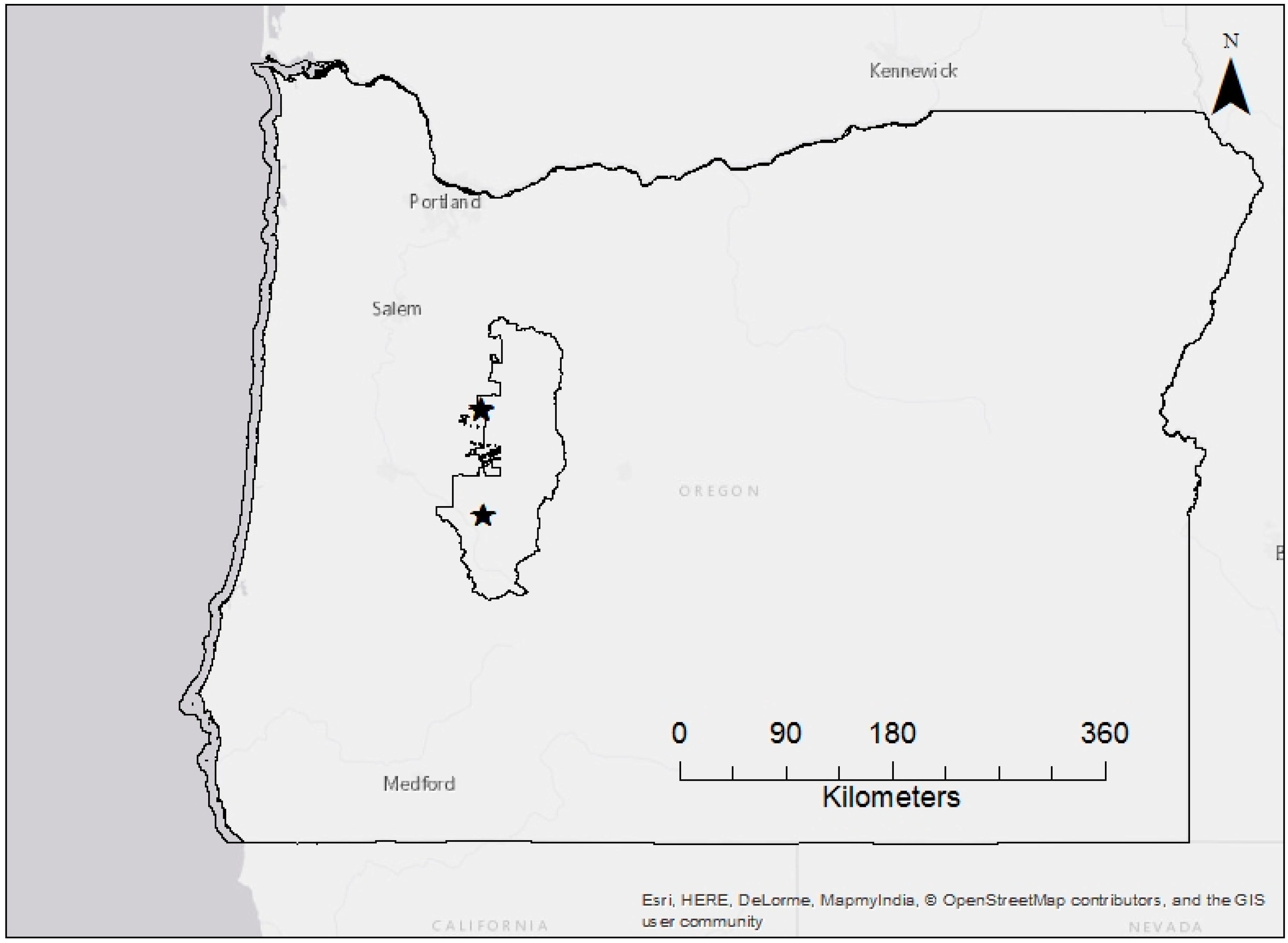
This study was carried out in the Willamette National Forest, an approximately 678,013-ha area that stretches for approximately 177 km along the western slopes of the Cascade Range (44°3′ N, 122°5′ W) in the western part of the U.S. state of Oregon. The elevation of the forest ranges from about 460 to 3200 m. About one-fifth of the forest, 154,106 ha, is designated for wilderness. Douglas fir is the dominant species with at least 15 other conifer species including hemlock, cedar, pine, and several species of fir common on the forest. The forest receives approximately 2000 to 3800 mm of annual rainfall, and the average annual temperature ranges from 5 to 19 °C. The forest has diverse soils, but their parent material is of volcanic origin. The locations of stands from which the sample trees were selected are shown in Figure 1.

2.2. Data

Detailed biomass data was collected by destructively sampling 14 red alder (Alnus rubra Bong.) and 12 Western hemlock (Tsuga heterophylla (Raf.) Sarg.) trees. The fieldwork was carried out between the first week of July and the third week of September in 2013. Tree level attributes such as DBH, total height, crown base height (height to the base of the first live branch), crown width, and main stem diameter at 0.15 m (stump height), 0.76 m, 1.37 m (breast height), and 2.4 m above ground, and every 1.22 m afterwards, were recorded. The average DBH was 27.1 cm (range 16.3–51.8 cm) and 44.7 cm (range 18.0–69.9 cm), and average height was 23.7 m (range 12.8–31.6 m) and 31.3 m (range 14.4 m–39.8 m), for red alder and Western hemlock trees, respectively.

A total of nine (four, three, and two from bottom, middle, and top equal-length stratums of sample trees) first-order branches, i.e., the branches that are directly attached to the main stem, per tree were randomly selected to obtain separate oven dry weights of branch wood and foliage. Individual branch wood and foliage biomass was obtained by fitting a species-specific log linear model as a function of branch diameter.

Stem wood and bark biomass was based on 3–5-cm-thick disks taken from the top of the stump and every 5.18 m. Stem wood biomass was calculated by multiplying the volume of each 5.18-m section by the average density of the disks taken from two ends, whereas stem bark biomass was based on the bark volume and bark density of the bark sample taken from the disks. Total stem wood and stem bark biomass was obtained by summing respective section masses. For details of the component and total biomass calculation process, refer to [12]. A summary of the data used in this study is presented in

Table 1. Summary statistics of tree data used in this study. CV is the coefficient of variation.

Variable	Minimum	Mean	Maximum	CV
Western hemlock
Foliage (kg)	10.0	77.6	184.0	0.82
Branch (kg)	20.0	236.7	609.0	0.97
Bark (kg)	4.0	62.1	147.0	0.76
Bole (kg)	72.0	1122.7	2512.0	0.76
Total (kg)	106.0	1499.0	3446.0	0.78
DBH (cm)	18.0	44.7	69.9	0.40
Total Height (m)	14.4	31.3	39.8	0.29
Red alder
Foliage (kg)	1.0	3.5	15.0	1.06
Branch (kg)	15.0	69.4	445.0	1.64
Bark (kg)	3.0	24.8	85.0	0.91
Bole (kg)	53.0	303.9	1129.0	0.95
Total (kg)	80.0	401.6	1674.0	1.05
DBH (cm)	16.3	27.1	51.8	0.37
Total Height (m)	12.8	23.7	31.6	0.23

.

2.3. Methods

We used two different approaches to estimate total and component biomass in Western hemlock and red alder trees. In the first approach, we fit a simultaneous system of component biomass equations with a seemingly unrelated regression (SUR). In the second approach, total AGB was first predicted as a function of DBH and total tree height using a linear model. The proportion of biomass in different aboveground components was predicted using beta, Dirichlet, and MLL regressions. The actual amount of component biomass was then obtained by distributing the predicted value of total AGB using predicted proportions in different regressions.

2.3.1. Seemingly Unrelated Regression (SUR)

The SUR model was first introduced by [14] and by [15] in biomass estimations to ensure the additivity of nonlinear biomass equations. Usually, the component models are fitted as a system of equations, and the equation for total AGB is constrained such that the prediction from the total AGB equation is compatible with the sum of the predicted values of the component biomass equations. Since the error terms in different component biomass equations are correlated, a SUR allows more efficient parameter estimation than an ordinary least squares regression [15]. We fitted a nonlinear system of equations using a constrained SUR. The equations for component and total AGB were in the following form:

$$BOL=exp\left(a_{11}+a_{12}{X}_1+a_{13}{X}_2\right)+e_1$$

(1)

$$BRK=exp\left(a_{21}+a_{22}{X}_1+a_{23}{X}_2\right)+e_2$$

(2)

$$BCH=exp\left(a_{31}+a_{32}{X}_1+a_{33}{X}_2\right)+e_3$$

(3)

$$FOL=exp\left(a_{41}+a_{42}{X}_1+a_{43}{X}_2\right)+e_4$$

(4)

$$TOT={\sum }_{i,j}exp\left(a_{ij}+a_{ij}{X}_1+a_{ij}{X}_2\right)+e_5$$

(5)

where, BOL, BRK, BCH, FOL, and TOT are bole, bark, branch, foliage, and total AGB, respectively, a_ij, (i = 1, 2, 3, 4, and j = 1, 2, 3) are parameters to be estimated from the data, and X₁ and X₂ are natural logarithms of DBH and total tree height, respectively. The SAS procedure PROC MODEL [16] was used to fit SUR models.

2.3.2. Beta Regression

A normal error regression assumes that the dependent variable lies in the real line and therefore may not be appropriate when the dependent variable is restricted to (0, 1) intervals such as percentage, proportion, and fraction or rate. If the dependent variable is a univariate continuous variable bounded between 0 and 1; the obvious choice of error distribution is the beta distribution because it has the same bounds. Beta regression in forestry has been used by [17] to model the percentage of canopy cover, by [18] to estimate the riparian percentage of shrub cover, and by [19] in modeling the percentage of tree canopy cover. Recently, [12] used the beta regression to estimate the proportion of biomass in different aboveground components in Douglas fir and lodgepole pine trees.

Beta density for modeling purposes has been described in the form of Equation (6) by [20].

$$f\left(y; \mu , \varphi \right)=\frac{\Gamma \left(\varphi \right)}{\Gamma \left(\mu \varphi \right)\Gamma \left(\left(1-\mu \right)\varphi \right)}{y}^{\mu \varphi -1}{\left(1-y\right)}^{\left(1-\mu \right)\varphi -1}, 0<\mathrm{y}<1$$

(6)

where, 0 < μ < 1 and φ > 0, with E(y) = μ and $Var\left(y\right)=\frac{\mu \left(1-\mu \right)}{1+\varphi }$.

Beta regression is an extension of generalized linear models and ensures the logical prediction of percentages [17]. The beta regression model can be written as:

$$g\left({\mu }_i\right)={\mathbf{x}}_i^{\mathrm{T}}\mathit{\beta }={\mathit{\eta }}_i$$

(7)

where, g(·) is strictly the increasing double differentiable link function that maps (0, 1) into the real line ℝ, ${\mathbf{x}}_i={\left(x_{i1},\dots \dots \dots ,x_{ik}\right)}^{\mathrm{T}}$ is a vector of k explanatory variables, $\mathit{\beta }={\left({\beta }_1,\dots \dots \dots ,{\beta }_k\right)}^{\mathrm{T}}$ is a vector of regression coefficients, and ${\mathit{\eta }}_i$ is a linear predictor (i.e., ${\mathit{\eta }}_i={\beta }_1{x}_{i1}+\dots +{\beta }_k{x}_{ik}$, usually $x_{i1}=1$ for all i, so that the model has an intercept) [21]. The logit link function $g\left(\mu \right)=\text{log}\left(\frac{\mu }{1-\mu }\right)$ was used; thus, the predicted values are obtained as ${\mu }_i=\frac{exp\left({\eta }_i\right)}{1+\text{exp}\left({\eta }_i\right)}$ . Parameter estimation is based on the method of maximum likelihood and was performed in R 3.2.3 [22] with function betareg in library betareg [21].

2.3.3. Dirichlet Regression

The Dirichlet regression is useful when the dependent variable is a vector of proportions that represent the components as a percentage of the total so that the component proportions sum to 1. It is assumed that the dependent variable follows a Dirichlet distribution, a multivariate generalization of the beta distribution having the general form:

$$f\left(\mathit{y};\mathit{\alpha }\right)=\frac{1}{\mathrm{B}\left(\mathit{\alpha }\right)}{\prod }_{c=1}^C{y}_c^{\left({\alpha }_c-1\right)}$$

(8)

where α_c > 0, ∀ c are the shape parameters for each components, $y_c\in \left(0,1\right)$ and ${\sum }_{c=1}^C{y}_c=1$. $\mathrm{B}\left({\alpha }_c\right)=\frac{{\prod }_{c=1}^C\Gamma \left({\alpha }_c\right)}{\Gamma \left({\sum }_{c=1}^C{\alpha }_c\right)}$ is the multinomial beta function, and Γ(·) is the gamma function. The Dirichlet distribution reduces to the beta distribution when there are only two components. [23] used similar parameterization of [20] to represent the Dirichlet distribution as follows:

$$f\left(\mathit{y};\mathit{\mu }, \varphi \right)=\frac{1}{\mathrm{B}\left(\mathit{\mu }\varphi \right)}{\prod }_{c=1}^C{y}_c^{\left({\mu }_c\varphi -1\right)}$$

(9)

where 0 < μ_c < 1 and φ > 0 (${\mu }_c=\frac{{\alpha }_c}{\varphi }$ and $\varphi ={\alpha }_0={\sum }_{c=1}^C{\alpha }_c$ are mean and precision parameters, respectively). The regression model for mean is then formulated as follows:

$$g_{\mu }\left({\mu }_c\right)={\eta }_{\mu c}=\mathit{X}{\beta }_c$$

(10)

where $g_{\mu }(·)$ is the link-function; with the logit link function, the predicted values are calculated as ${\mu }_r=\frac{1}{1+{\sum }_{a=1}^C\text{exp}\left(\mathit{X}{\beta }_a\right)}$ for the reference component and ${\mu }_c=\frac{\text{exp}\left(\mathit{X}{\beta }_a\right)}{1+{\sum }_{a=1}^C\text{exp}\left(\mathit{X}{\beta }_a\right)}$ for other components. For the details of parameterization of Dirichlet distribution and the method of parameter estimation in the Dirichlet regression, refer to [23]. The Dirichlet regression was performed in R 3.2.3 [22] with function DirichReg in library DirichletReg [23], using component bole as the reference group (choice of a reference group is arbitrary).

2.3.4. Multinomial Log-linear Regression

The data formatting and model formulation in the MLL regression followed the same approach as described in [12]. Four components of aboveground biomass (bole, bole bark, branch, and foliage) were first set to four nominal values. Then, the models to predict proportions of total tree biomass found in bole, bole bark, branch, and foliage were fit simultaneously using a multinomial logit model. The predicted probabilities of multinomial logit fit can be considered as the proportion of biomass in each component [8]. The resulting prediction equations for component proportions are:

$$p_{BOL}=\frac{1}{1+e^{\left(a_1+a_2{X}_1+a_3{X}_2\right)}+e^{\left(b_1+b_2{X}_1+b_3{X}_2\right)}+e^{\left(c_1+c_2{X}_1+c_3{X}_2\right)}}$$

(11)

$$p_{BRK}=\frac{e^{\left(a_1+a_2{X}_1+a_3{X}_2\right)}}{1+e^{\left(a_1+a_2{X}_1+a_3{X}_2\right)}+e^{\left(b_1+b_2{X}_1+b_3{X}_2\right)}+e^{\left(c_1+c_2{X}_1+c_3{X}_2\right)}}$$

(12)

$$p_{BCH}=\frac{e^{\left(b_1+b_2{X}_1+b_3{X}_2\right)}}{1+e^{\left(a_1+a_2{X}_1+a_3{X}_2\right)}+e^{\left(b_1+b_2{X}_1+b_3{X}_2\right)}+e^{\left(c_1+c_2{X}_1+c_3{X}_2\right)}}$$

(13)

$$p_{FOL}=\frac{e^{\left(c_1+c_2{X}_1+c_3{X}_2\right)}}{1+e^{\left(a_1+a_2{X}_1+a_3{X}_2\right)}+e^{\left(b_1+b_2{X}_1+b_3{X}_2\right)}+e^{\left(c_1+c_2{X}_1+c_3{X}_2\right)}}$$

(14)

where p_BOL, p_BRK, p_BCH, and p_FOL are proportions of total aboveground biomass in bole, bark, foliage, and branch, respectively; X₁ = DBH; X₂ = total tree height; and a_i, b_i, c_i (i = 1, 2, 3) are regression coefficients to be estimated from the data. The MLL regression was performed in R 3.2.3 [22] with function multinom in library nnet [24], using component bole as the reference group. The amount of biomass present in each component was used as the frequency weight.

2.4. Evaluation

Performance of these methods were compared using bias, bias percent, RMSE, RMSE percent, and R² values calculated as follows:

$$Bias=\frac{{\sum }_{i=1}^n\left(y_i-\widehat{y_i}\right)}{n}$$

(15)

$$Bias Percent=100\times \frac{Bias}{\overline{y}}$$

(16)

$$RMSE=\sqrt{\frac{{\sum }_{i=1}^n{\left(y_i-\widehat{y_i}\right)}^2}{n}}$$

(17)

$$RMSE Percent=100\times \frac{RMSE}{\overline{y}}$$

(18)

$$R^2=1-\frac{{\sum }_{i=1}^n{\left(y_i-{\widehat{y}}_i\right)}^2}{{\sum }_{i=1}^n{\left(y_i-\overline{y}\right)}^2}$$

(19)

where y_i and $\widehat{y_i}$ are the observed and predicted biomass, respectively, in the i^th tree, and $\overline{y}$ is the average biomass of n trees.

3. Results and Discussion

The majority of the aboveground biomass was contained in the bole component for both species. It ranged from 63.9% to 83.1% (74.7% on average) of AGB in Western hemlock trees and from 66.2% to 86.6% (77.4% on average) in red alder trees. Bark accounted for the smallest proportion of AGB in Western hemlock, ranging from 3.5% to 5.3%, whereas, for red alder, foliage was the component with the smallest proportion, accounting for only 0.2% to 2.6% of AGB. Branch and foliage biomass in Western hemlock ranged from 8.4% to 23.6% and 3.1% to 9.4%, respectively. In red alder trees, branch and bark biomass ranged from 4.7% to 27.5% and 3.8% to 8.4% of AGB, respectively. All regression methods to predict biomass were applied to both species.

3.1. Seemingly Unrelated Regression (SUR)

The estimated correlation matrix of residuals obtained from the SUR model fit for Western hemlock (corr_WH) and red alder (corr_RA) biomass equations were:

$$cor{r}_{WH}\left(e_i\right)=\left[\begin{array}{ccccc}1& -0.17& -0.84& -0.75& 0.71\\ & 1& -0.10& -0.30& -0.40\\ & & 1& 0.97& -0.21\\ & & & 1& -0.10\\ & & & & 1\end{array}\right]$$

(20)

and

$$cor{r}_{RA}\left(e_i\right)=\left[\begin{array}{ccccc}1& 0.18& 0.60& 0.31& 0.95\\ & 1& -0.50& 0.69& 0.003\\ & & 1& -0.22& 0.81\\ & & & 1& 0.21\\ & & & & 1\end{array}\right]$$

(21)

Both positive and negative correlations among model residuals were observed. Cross-equation error correlation in Western hemlock models ranged from −0.84 (between branch and bole) to 0.97 (between branch and foliage), whereas, in red alder models, it ranged from −0.50 (between branch and total) to 0.95 (between bole and total). Parameter estimates and their approximate standard errors for SUR models are given in

Table 2. Parameter estimates and their approximate standard errors (SE) for the component and total aboveground biomass models for red alder and Western hemlock trees. Model forms for component and total aboveground biomass (AGB) are given in Equations (1)–(5).

Parameter	Western Hemlock		Red Alder
	Estimate	Approx. SE	Estimate	Approx. SE
a11	−3.49438	0.45210	−5.51855	0.91800
a12	1.52803	0.06720	1.65452	0.14530
a13	1.31316	0.14160	1.73720	0.39850
a21	−6.03297	0.61420	−5.08327	1.24330
a22	1.87054	0.10090	1.47381	0.27690
a23	0.82538	0.17900	1.06642	0.57770
a31	−7.65133	0.96880	−29.01600	7.24370
a32	3.85302	0.21180	2.32864	0.89350
a33	−0.61311	0.20620	7.50781	3.00380
a41	−7.29448	1.14550	0.93047	3.18410
a42	2.90439	0.21740	2.03755	1.79700
a43	0.05529	0.29450	−1.89664	2.16760

. The foliage model for red alder performed very poorly (Adjusted − R² = 0.30) compared to the models for other components. We do not have a good explanation for the smaller variation indicated by the foliage model, but it is possible that the smaller values of foliage biomass compared to the biomass in other components impacted the estimation. There are two options one could achieve foliage biomass estimation: (1) fit the foliage model outside of the system or (2) combine the foliage and branch wood as one component, which is probably less desirable. When the foliage model for red alder was fitted outside of the system, the Adjusted − R² increased to 0.77 without impacting the fit of other components in the system of equations. The evaluation statistics produced by SUR models in estimating component and total aboveground biomass are presented in

Table 3. Evaluation statistics (bias, bias percent, root mean square error (RMSE), and RMSE percent) in component biomass estimation in Western hemlock and red alder trees using seemingly unrelated regression (SUR).

Component	Bias (kg)	Bias Percentage	RMSE (kg)	RMSE Percentage
Western Hemlock
Bole	−20.26	−1.80	63.45	5.65
Bark	−0.03	−0.06	4.33	6.98
Branch	14.56	6.15	33.90	14.32
Foliage	5.07	6.54	12.59	16.23
Total	−0.66	−0.04	34.97	2.33
Red Alder
Bole	5.00	1.64	26.82	8.83
Bark	−2.16	−8.73	3.92	15.82
Branch	10.93	15.75	21.97	31.64
Foliage	−1.88	−53.74	2.93	83.69
Total	11.88	2.96	43.78	10.90

. Our evaluation statistics are based on the SUR system that includes the foliage biomass equation. It was evident that the prediction of biomass in Western hemlock was more accurate in terms of bias and RMSE compared to the prediction in red alder. More complex allometric equations are likely needed to improve the accuracy of biomass equations for hardwoods. Power models are commonly used in biomass estimation. However, the power models did not perform as well as the models we have used (Equations (1)–(5)). Due to the smaller sample size, we did not try very complex models. Even though biomass models are commonly faced with heterogeneous error variance, residual analysis in our study did not show any pattern of heteroscedasticity. The problem of heteroscedasticity, if present, can be resolved by using a weighted regression. Discussion on approaches to find an appropriate weight function for nonlinear biomass models can be found in [25]. We would like to note that some of the parameter estimates for red alder component models obtained from SUR are “unusual”, specifically coefficient a₃₁. We tried several starting values to make sure that the minimization attained the global minimum. However, the parameter estimates were stable. One reason for “unusual” parameter estimates could be due to the smaller sample size available for model fitting.

3.2. Regressions to Predict Proportion

The estimation of proportion itself does not provide any value without the estimate for total aboveground biomass. Observed total aboveground biomass could have been used for the sample data, but that does not provide any significance for future applications. Therefore, a linear model relating total aboveground biomass with DBH and height (Equation (22)) was first fitted. Parameter estimates and the index of fit (Adjusted − R²) of this model for both species are given in

Table 4. Parameter estimates and their standard errors for the log–log model (Equation (22)) to estimate total aboveground biomass in Western hemlock and red alder trees. CF is the log-bias correction factor calculated as $\text{exp}\left(\frac{\text{MSE}}{2}\right)$.

Species	Parameter Estimates (S.E.)			Adjusted-R2	CF
	a	b	c
Western Hemlock	−3.41345 (0.12227)	1.93633 (0.05889)	0.90878 (0.07164)	0.9986	1.0009
Red Alder	−3.62175 (0.40260)	1.90612 (0.15135)	0.97674 (0.19756)	0.9808	1.0070

.

$$\text{ln}\left(AGB\right)=a+b\ast \text{ln}\left(DBH\right)+c\ast \text{ln}\left(HT\right)+e$$

(22)

AGB in original scale, using this model, can be calculated as $AGB=a_{0}DB{H}^{b}H{T}^c$, where $a_0=CF\times exp\left(a\right)$. Adjusted − R² of the original models were 0.9985 and 0.9653 for Western hemlock and red alder, respectively.

The proportion of biomass in different aboveground components were related to DBH and height through beta, Dirichlet, and MLL regressions. The independent variables were used in their original form in proportion models because they provided better fit compared with the models with log-transformed independent variables. In beta regression, different component proportions are fitted independently of each other. The Pseudo − R² (an R²-like measure calculated based on estimated likelihood) values of beta regression ranged from 0.3562 (bark model) to 0.8305 (bole model) for Western hemlock and 0.6093 (bark model) to 0.7164 (bole model) for red alder trees (

Table 5. Parameter estimates and pseudo-R² values for the component biomass models for Western hemlock and red alder trees using beta regression.

Model	Parameter Estimates			Pseudo-R2
	Intercept	DBH	HT
Western Hemlock
Bole	0.30314	−0.02093	0.05554	0.8305
Bark	−3.33911	−0.00436	0.01243	0.3562
Branch	−0.95380	0.02793	−0.06525	0.8281
Foliage	−1.85514	0.00911	−0.04418	0.7244
Red Alder
Bole	0.28216	−0.04399	0.09147	0.7164
Bark	−3.67702	−0.02044	0.06254	0.6093
Branch	−0.35253	0.06547	−0.13526	0.6986
Foliage	−2.15422	0.02285	−0.12946	0.6472

). The evaluation statistics produced by the beta regression models are given in

Table 6. Evaluation statistics (Bias, bias percent, RMSE, and RMSE percent) in component biomass estimation in Western hemlock and red alder trees using beta regression.

Component	Bias	Bias Percentage	RMSE	RMSE Percentage
Western Hemlock
Bole	−1.08	−0.10	62.41	5.56
Bark	−0.18	−0.29	6.07	9.78
Branch	1.67	0.70	29.36	12.41
Foliage	0.90	1.15	12.56	16.19
Red Alder
Bole	0.34	0.11	36.97	12.17
Bark	−0.41	−1.67	2.42	9.75
Branch	5.71	8.23	37.21	53.60
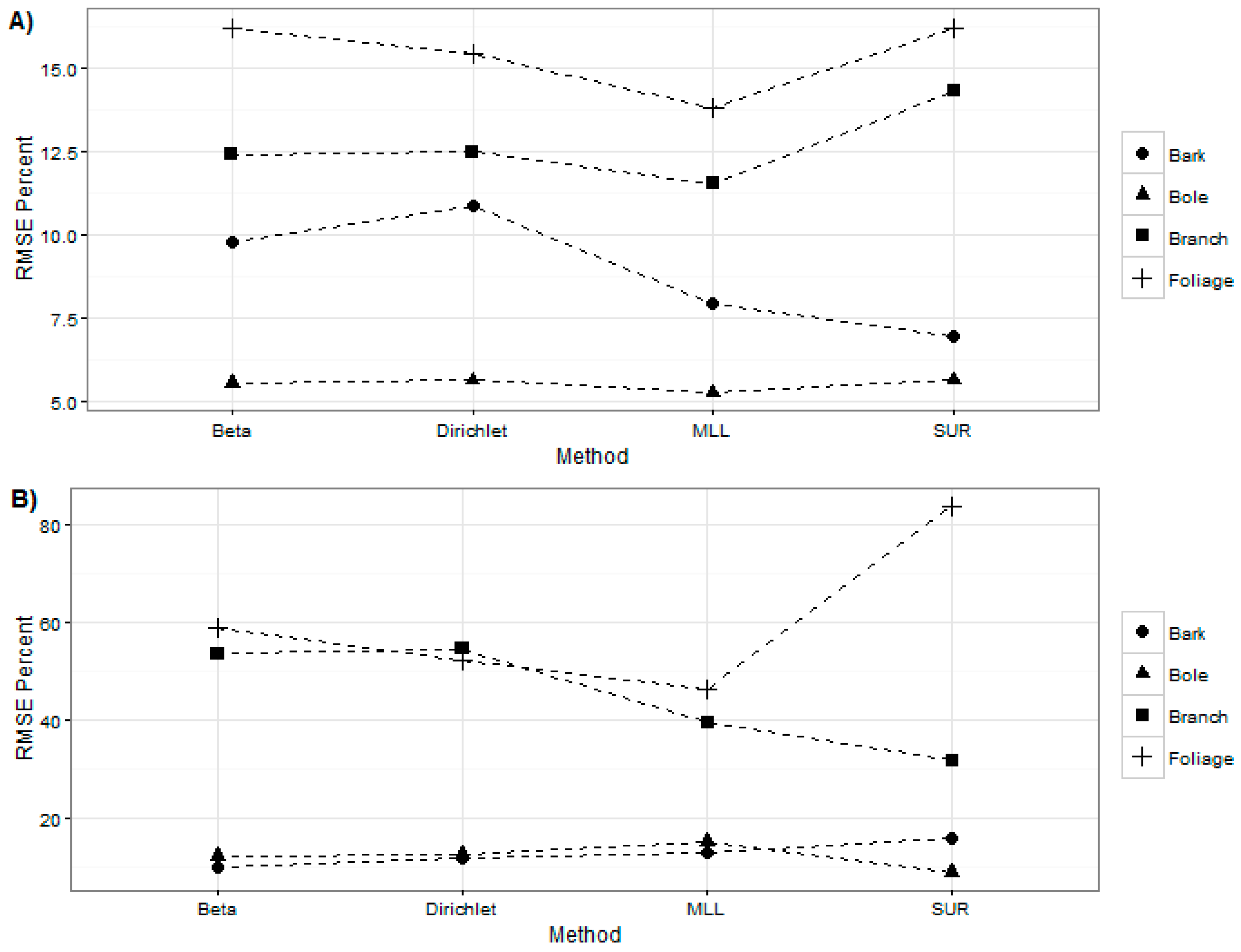
Foliage	0.27	7.60	2.05	58.72

. The root mean squared errors of the beta regression models for Western hemlock were similar to those obtained from the SUR models. However, for the red alder trees, the results were variable. Foliage and bark models in beta regression reduced RMSE by 25% and 6%, but, for branch and bole biomass, the beta regression produced RMSEs that were respectively 22% and 3% higher than that produced by the SUR models.

In Dirichlet and MLL regressions, the component proportions are fitted simultaneously, which ensures that the predicted proportions sum to 1. Parameter estimates obtained from the Dirichlet regressions were different from those obtained from beta regression (Table 5 vs.

Table 7. Parameter estimates for the component biomass models for Western hemlock and red alder trees from using the Dirichlet regression. Component bole was used as reference group for both species.

Model	Parameter Estimates
	Intercept	DBH	HT	R2
Western Hemlock
Bark	−2.84835	0.00112	−0.00258	0.2788
Branch	−0.74079	0.02901	−0.06969	0.8665
Foliage	−1.46896	0.01408	−0.05603	0.8323
Red Alder
Bark	−3.16541	−0.00886	0.03701	0.5689
Branch	−0.25335	0.06685	−0.13813	0.7397
Foliage	−1.76809	0.03266	−0.13995	0.7374

). Similar to beta regression, the amount of variation explained by the Western hemlock bark model in the Dirichlet regression was very low (0.2788) compared to other models (0.8323 and 0.8665 for foliage and branch models, respectively). The evaluation statistics produced by the Dirichlet regression are presented in

Table 8. Evaluation statistics (Bias, bias percent, RMSE, and RMSE percent) in component biomass estimation in Western hemlock and red alder trees using the Dirichlet regression.

Component	Bias	Bias Percentage	RMSE	RMSE Percentage
Western Hemlock
Bole	−0.89	−0.08	63.51	5.66
Bark	−1.07	−1.73	6.75	10.87
Branch	2.49	1.05	29.59	12.50
Foliage	0.60	0.78	12.00	15.46
Red Alder
Bole	0.22	0.07	38.01	12.51
Bark	−1.06	−4.30	2.93	11.83
Branch	6.79	9.78	37.86	54.54
Foliage	−0.35	−10.09	1.83	52.31

. RMSEs for the Dirichlet regression models for Western hemlock were within 15% for all components. The RMSEs for bole and bark biomass estimation was 12.5% and 11.8%, respectively, for red alder trees, whereas the RMSEs for foliage and branch biomass estimation was 52.3% and 54.4%, respectively.

The parameter estimates obtained from the MLL regression are presented in

Table 9. Parameter estimates for the component biomass models for Western hemlock and red alder trees using multinomial log-linear regression model. Component bole was used as reference group for both species.

Model	Parameter Estimates
	Intercept	DBH	HT	R2
Western Hemlock
Bark	−2.65312	0.00333	−0.01191	0.2959
Branch	−0.99468	0.02917	−0.06261	0.8667
Foliage	−1.82478	0.01372	−0.04527	0.8326
Red Alder
Bark	−3.07429	−0.01258	0.03696	0.5495
Branch	−0.40701	0.07676	−0.14342	0.7327
Foliage	−1.64322	0.05711	−0.18088	0.6863

, and evaluation statistics are given in

Table 10. Evaluation statistics (Bias, bias percent, RMSE, and RMSE percent) in component biomass estimation in Western hemlock and red alder trees using multinomial log-linear regression.

Component	Bias	Bias Percentage	RMSE	RMSE Percentage
Western Hemlock
Bole	0.64	0.06	59.08	5.26
Bark	0.04	0.07	4.93	7.94
Branch	0.37	0.16	27.32	11.54
Foliage	0.08	0.10	10.70	13.79
Red Alder
Bole	3.00	0.99	45.89	15.10
Bark	0.21	0.83	3.19	12.88
Branch	2.34	3.37	27.40	39.47
Foliage	0.05	1.40	1.61	46.12

. Even though the form of the prediction equations for Dirichlet and MLL regressions are the same, parameter estimates obtained from these two methods were different (Table 7 vs. Table 9). In comparison to the Dirichlet regression, the MLL models reduced RMSEs by 1.7%, 2.9%, 1.0% and 0.4% for foliage, bark, branch, and the bole biomass estimation of Western hemlock. For the red alder trees, the MLL regression models reduced RMSEs by 6.2% and 15.1% for foliage and branch biomass estimation but it produced 1.1% and 2.6% higher RMSE for bark and bole biomass estimation, respectively. Figure 2 shows the complete comparison of percentage root mean squared error obtained by using different methods to estimate components of AGB.

4. Conclusions

We fitted DBH- and height-based biomass equations for Western hemlock and red alder trees using different regression approaches. Even though a method that is consistently better than others is desired, none of the methods we used was a clear winner when all methods (SUR, beta, Dirichlet, and MLL) were compared to one another. Accuracy of these methods differed between species, with higher root mean square error being produced in red alder trees, for which more complex models than the models for conifers might be required. Within species, the accuracy of the equation for bole biomass was better than the equations for other components. Total AGB can be estimated with high accuracy using a simple linear model that related the logarithm of AGB to the logarithms of DBH and height (Adjusted − R² 0.99 and 0.97, for the untransformed model, and RMSE 2.47 and 18.82% for Western hemlock and red alder, respectively) and distributed to different components using the proportions predicted through beta, Dirichlet, and MLL regressions.

The beta regression can be used to fit independent proportion models, and Dirichlet and MLL regressions can be used to simultaneously fit proportion models. Predicted values of proportions in beta regression may not sum to 1. In that case, one can fit C − 1 equations, where C is the number of components, and calculate the proportion of remaining components by subtraction or, alternatively, by dividing the predicted proportion in each component by the sum of all predicted proportions. Methods to predict proportions are promising because they satisfy the assumption of error distribution. The measures of fit obtained from these methods (R² and Pseudo − R²) were very high compared to the R² values of the Jenkins equations for component ratios. The Dirichlet and MLL regressions have an additional attractive property of the unit sum of predicted proportions. We further prefer the Dirichlet regression to MLL because MLL requires a non-standard data processing and actually produces the probabilities of a nominal variable occurring [8]. On the other hand, given the fact that more than 70% of biomass, on average, is contained in the main stem, the choice of biomass equations should be governed by the objective of management. For our relatively small dataset, the methods to predict proportion were unbiased and should be tested with a larger sample size.