
Geospatial Estimation of above Ground Forest Biomass in the Sierra Madre Occidental in the State of Durango, Mexico

 , ,
, ,
Abstract
:1. Introduction
2. Material and Methods
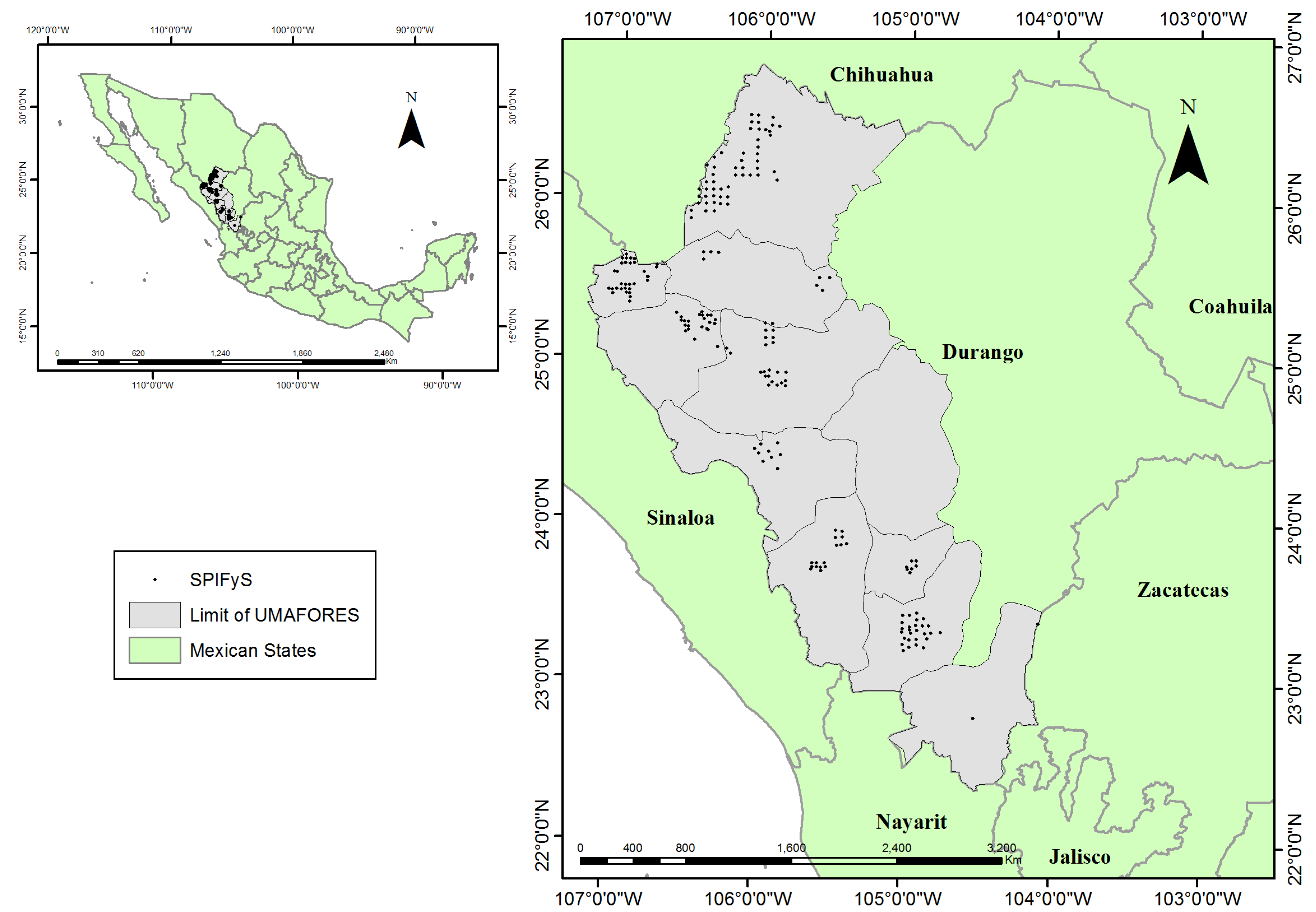
2.1. Study Area
2.2. Field Data
2.3. Tree Abundance by Species Group (ASG)
2.4. Source of Spectral Data
2.5. Integration of Data Files
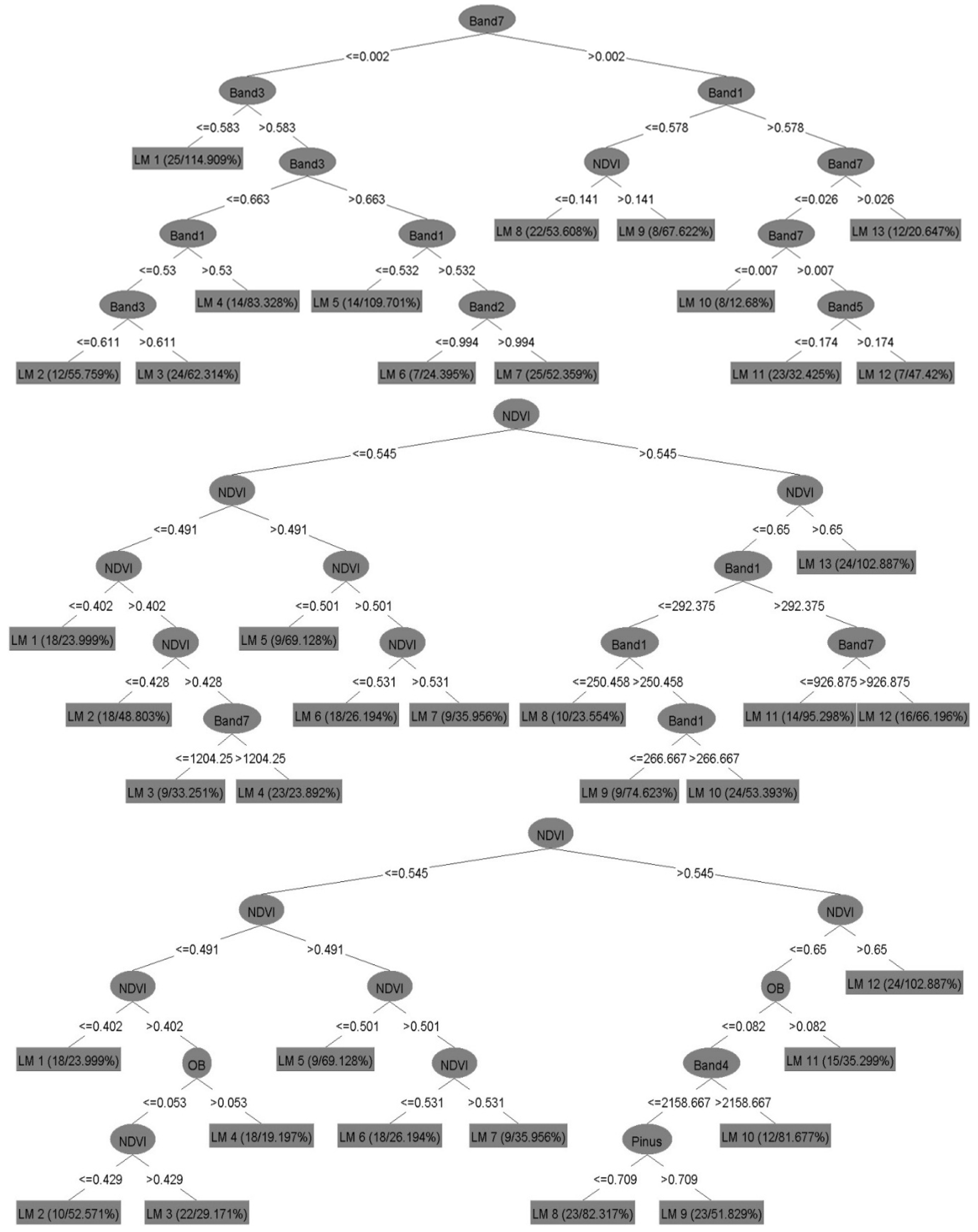
2.6. Fitted Model
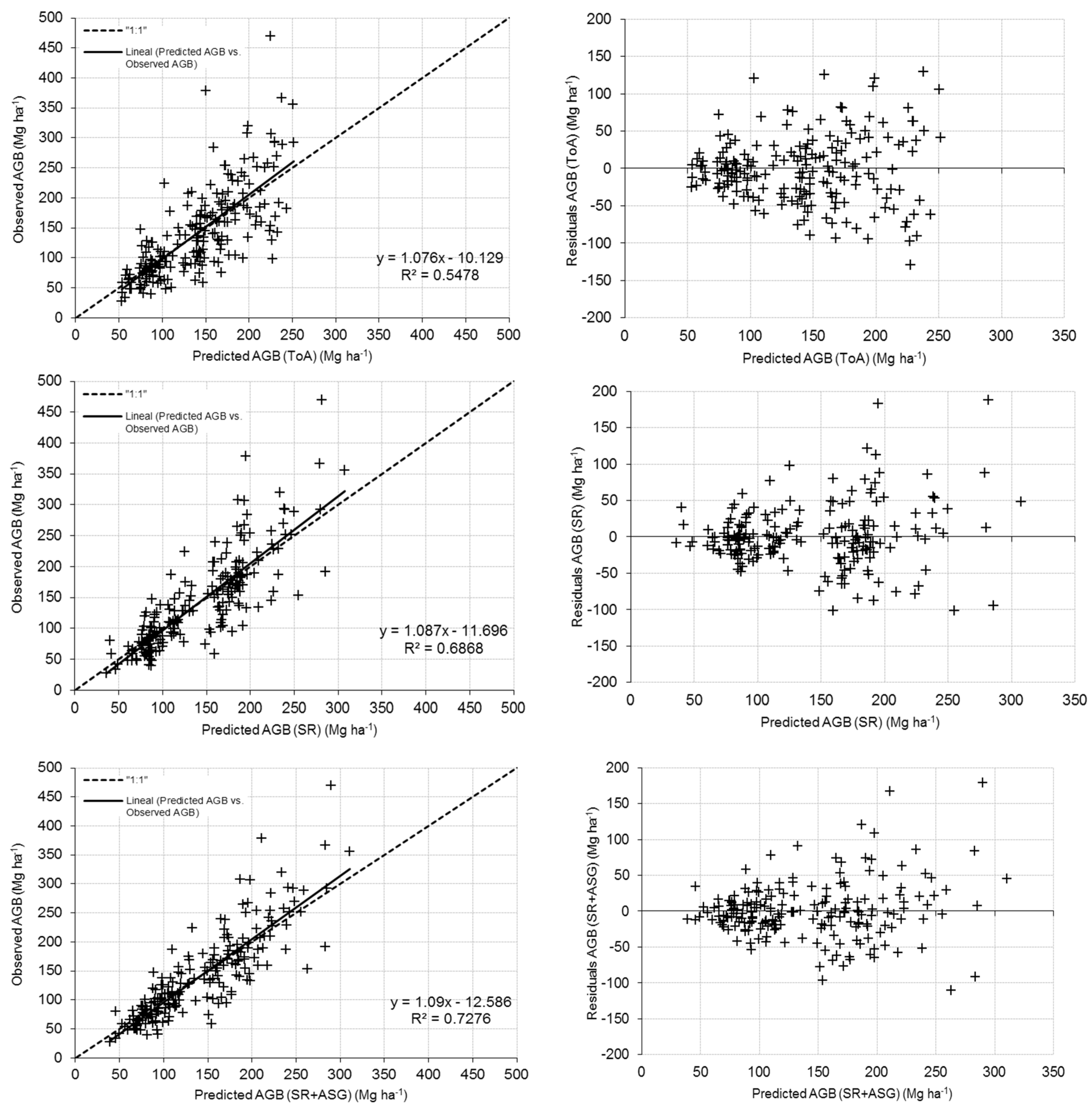
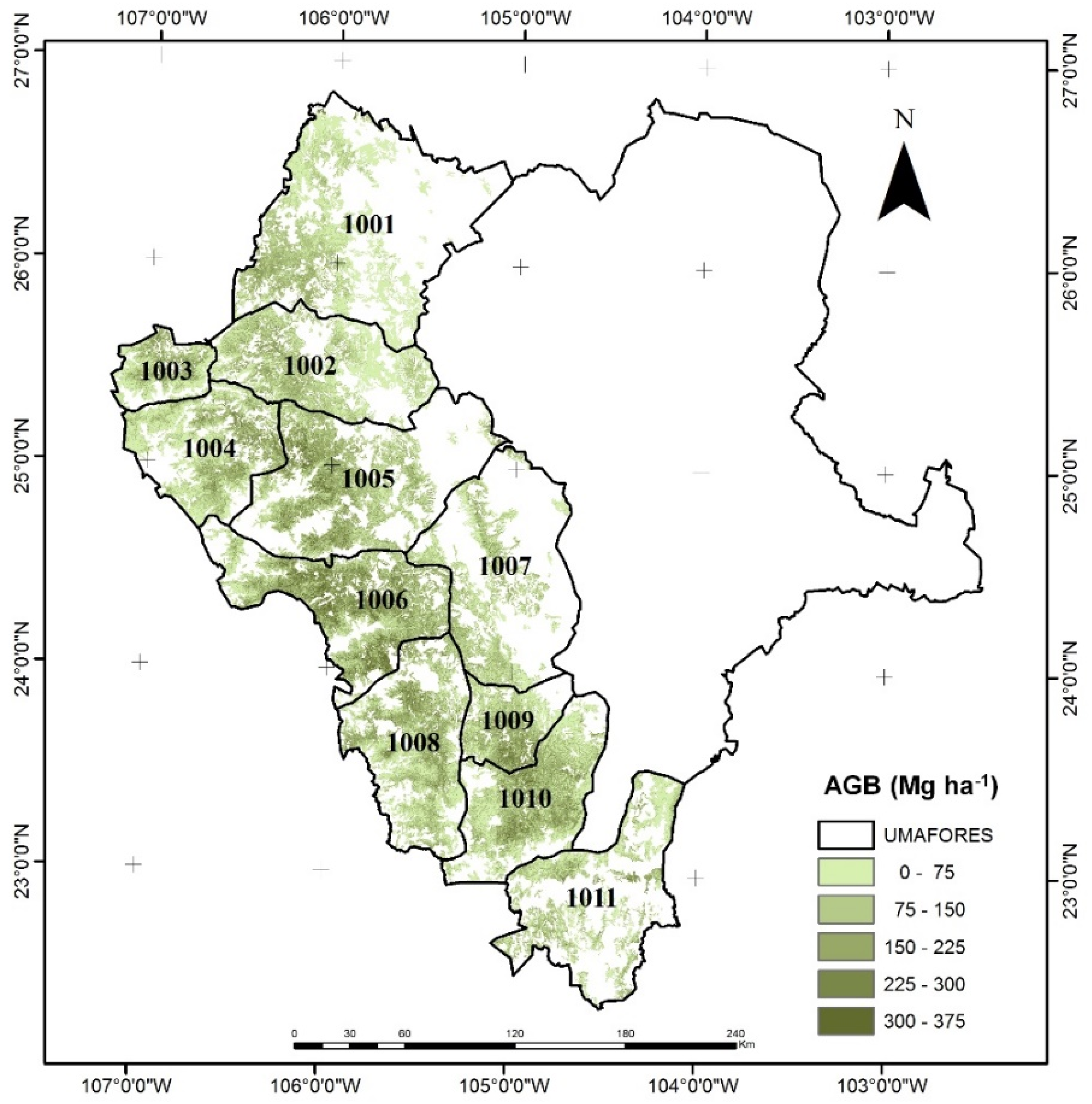
3. Results
4. Discussion
5. Conclusions
Acknowledgments
Author Contributions
Conflicts of Interest
References
- González Elizondo, M.S.; González Elizondo, M.; Tena Flores, J.A.; Ruacho González, L.; López-Enríquez, I.L. Vegetación de la Sierra Madre Occidental, México: una síntesis. Acta Botánica Mex. 2012, 100, 351–403. [Google Scholar]
- Sánchez, O.; Vega, E.; Peters, E.Y.; Monrroy, V.O. Conservación de Ecosistemas Templados de Montaña en México; Instituto Nacional de Ecología (INE–SEMARNAT): México D.F., México, 2003. [Google Scholar]
- Secretaría de Medio Ambiente y Recursos Naturales. Anuario Estadístico de la Producción Forestal 2011; México, 2011; pp. 11–24. [Google Scholar]
- Foody, G.M.; Boyd, D.S.; Cutler, M.E.J. Predictive relations of tropical forest biomass from Landsat TM data and their transferability between regions. Remote Sens. Environ. 2003, 85, 463–474. [Google Scholar] [CrossRef]
- Hall, R.J.; Skakun, R.S.; Arsenault, E.J.; Case, B.S. Modeling forest stand structure attributes using Landsat ETM+ data: Application to mapping of aboveground biomass and stand volume. For. Ecol. Manag. 2006, 225, 378–390. [Google Scholar] [CrossRef]
- Fuchs, H.; Magdon, P.; Kleinn, K.; Flessa, H. Estimating aboveground carbon in a catchment of the Siberian forest tundra: Combining satellite imagery and field inventory. Remote Sens. Environ. 2009, 113, 518–531. [Google Scholar] [CrossRef]
- Verbesselt, J.; Hyndman, R.; Newnham, G.; Culvenor, D. Detecting trend and seasonal changes in satellite image time series. Remote Sens. Environ. 2010, 114, 106–115. [Google Scholar] [CrossRef]
- Barajas, F.H. Comparación Entre Análisis Discriminante no-Métrico y Regresión Logística Multinomial. Tesis de Maestría, Facultad de Ciencias, Universidad Nacional de Colombia, Medellín, Colombia, 2007. [Google Scholar]
- Gibbons, J.D.; Chakraborti, S. Nonparametric Statistical Interference; Marcel Denker, Inc.: New York, NY, USA, 2003; p. 645. [Google Scholar]
- Karjalainen, M.; Kankare, V.; Vastaranta, M.; Holopainen, M.; Hyyppa, J. Prediction of plot-level forest variables using TerraSAR-X stereo SAR data. Remote Sens. Environ. 2012, 117, 338–347. [Google Scholar] [CrossRef]
- Quinlan, J.R. Learning with Continuous Classes. In 5th Australian Joint Conference on Artificial Intelligence; Word Scientific: Singapore, 1992; pp. 343–348. [Google Scholar]
- SRNyMA-CONAFOR. Plan Estrátegico Forestal 2030; Gobierno del estado de Durango: Durango, México, 2007. [Google Scholar]
- Zhao, X.; Corral-Rivas, J.J.; Zhang, C.; Temesgen, H.; Gadow, K. Forest observational studies-an essential infrastructure for sustainable use of natural resources. Forest Ecosyst. 2014. [Google Scholar] [CrossRef]
- Wehenkel, C.; Corral-Rivas, J.J.; Hernández-Díaz, J.C.; Gadow, K. Estimating Balanced Structure Areas in multi-species forests on the Sierra Madre Occidental, Mexico. Ann. For. Sci. 2011, 68, 385–394. [Google Scholar] [CrossRef]
- Corral Rivas, J.; Vargas, B.; Wehenkel, C.; Aguirre, O.; Álvarez, J.; Rojo, A. Guía para el Establecimiento de Sitios de Inventario Periódico Forestal y de Suelos del Estado de Durango; Facultad de Ciencias Forestales. Universidad Juárez del Estado de Durango: Durango, México, 2009. [Google Scholar]
- Vargas-Larreta, B.; González-Herrera, L.; López-Sánchez, C.A.; Corral-Rivas, J.J.; López-Martínez, J.O.; Aguirre-Calderón, C.G.; Álvarez-González, J.J. Biomass equations and Carbon content of the temperate forests of northwestern México. Biomass Bioenerg. 2015, in press. [Google Scholar]
- United States Geological Survey. Available online: http://glovis.usgs.gov (accessed on 11 January 2011).
- NASA. Landsat 7 Science Data Users Handbook, 2011. Available online: http://landsathandbook.gsfc.nasa.gov/pdfs/Landsat7_Handbook.pdf (accessed on 11 January 2011).
- Greenle, P.T. Remote Sensing science applications in arid environments. Remote Sens. Environ. 1993, 23, 143–154. [Google Scholar]
- Chuvieco, E. Teledetección Ambiental: La observación de la tierra desde el espacio, 3rd ed.; Ariel.: Barcelona, España, 2010; pp. 262–306. [Google Scholar]
- Keys, R.G. Cubic convolution interpolation for digital image processing. IEEE Trans. Acoust. Speech Signal Process. 1981, 29, 1153–1160. [Google Scholar] [CrossRef]
- Eastman, J.R. IDRISI, Selva., Guía para SIG y Procesamiento de Imágenes; Clark Labs Clark University: Worcester, MA, USA, 2012. [Google Scholar]
- Eastman, J.R. IDRISI version Selva, software for GIS and image processing; Clark University: Worcester, MA, USA, 2012.
- Gasparri, N.I.; Parmuchi, M.G.; Bono, J.; Karszenbaum, H.; Montenegro, C.L. Assessing multi-temporal Landsat 7 ETM+ images for estimating above-ground biomass in subtropical dry forests of Argentina. J. Arid Environ. 2010, 74, 1262–1270. [Google Scholar] [CrossRef]
- Liang, S.; Li, X.; Wang, J. Advanced Remote Sensing: Terrestrial Information Extraction and Applications; Academic Press: Oxford, UK, 2012. [Google Scholar]
- Zhu, X.; Liu, D. Improving forest aboveground biomass estimation using seasonal Landsat NDVI time-series. ISPRS J. Photogramm. Remote Sens. 2015, 102, 222–231. [Google Scholar] [CrossRef]
- ArcGIS for Desktop, version 10; software for analyzing geographic information systems; ESRI: Redlands, CA, USA, 1999–2012.
- Breiman, L.; Friedman, J.; Olshen, R.; Sone, C. Classification and Regression Trees; Wadsworth International Group: Belmont, CA, USA, 1984. [Google Scholar]
- Wang, Y.; Witten, I.H. Induction of model trees for predicting continuous classes. In Proceedings of the Poster Papers of the 9th European Conference on Machine Learning, Hamilton, New Zealand, 23 October 1997.
- Hall, M. Correlation-based Feature Selection for Machine Learning. Ph.D. Thesis, University of Waikato, Hamilton, New Zealand, 1999. [Google Scholar]
- Jakubauskas, M.E. Thematic Mapper characterization of lodge pole pine serals in Yellowstone National Park, USA. Remote Sens. Environ. 1996, 56, 118–132. [Google Scholar] [CrossRef]
- Huete, A.R.; Liu, H.; van Leeuwen, W.J. The Use of Vegetation Indices in Forested Regions: Issues of Linearity and Saturation. In Proceedings of 1997 IEEE International Geoscience and Remote Sensing Symposium, Singapore, 3–8 August 1997; European Space Agency Publications Division: Noordwijk, The Netherlands, 1997; pp. 1966–1968. [Google Scholar]
- Lu, D.; Mausel, P.; Brondızio, E.; Moran, E. Relationships between forest stand parameters and Landsat TM spectral responses in the Brazilian Amazon Basin. For. Ecol. Manag. 2004, 198, 149–167. [Google Scholar] [CrossRef]
- Mutanga, O.; Skidmore, A.K. Narrow band vegetation indices overcome the saturation problem in biomass estimation. Int. J. Remote Sens. 2004, 25, 3999–4014. [Google Scholar] [CrossRef]
- Fassnacht, K.S.; Gower, S.T.; MacKenzie, M.D.; Nordheim, E.V.; Lillesand, T.M. Estimating the leaf area index of North Central Wisconsin forests using the Landsat Thematic Mapper. Remote Sens. Environ. 1997, 61, 229–245. [Google Scholar] [CrossRef]
- Palestina, R.A.; Equihua, M.; Pérez-Maqueo, O.M. Influencia de la complejidad estructural del dosel en la reflectancia de datos Landsat TM. Madera y Bosques 2015, 21, 63–75. [Google Scholar]
- Günlü, A.; Ercanli, İ.; Başkent, E.Z.; Çakır, G. Estimating aboveground biomass using Landsat TM imagery: A case study of Anatolian Crimean pine forests in Turkey. Ann. For. Res. 2014, 57, 289–298. [Google Scholar]
- Houghton, R.A.; Butman, D.; Bunn, A.G.; Krankina, O.N.; Schlesinger, P.; Stone, T.A. Mapping Russian forest biomass with data from satellites and forest inventories. Environ. Res. Lett. 2007, 4, 1–7. [Google Scholar] [CrossRef]
- Tian, X.; Zengyuan, L.; Zhongbo, S.; Erxue, C.; Christiaan, T.; Xin, L.; Guo, Y.; Longhui, L.; Feilong, L. Estimating montane forest above-ground biomass in the upper reaches of the Heihe River Basin using Landsat-TM data. Int. J. Remote Sens. 2014, 35, 7339–7362. [Google Scholar] [CrossRef]
- Guoa, Y.; Tianb, X.; Lib, Z.; Linga, F.; Chenb, E.; Yanb, M.; Lib, C. Comparison of estimating forest above-ground biomass over montane area by two non-parametric methods. ISPRS J. Photogramm. Remote Sens. 2014, 92, 137–146. [Google Scholar]
- Foody, G.M.; Cutler, M.E.; Mcmorrow, J.; Pelz, D.; Tangki, H.; Boyd, D.S.; Douglas, I. Mapping the biomass of Bornean tropical rain forest from remotely sensed data Global. Ecol. Biogeogr. 2001, 10, 379–387. [Google Scholar] [CrossRef]
- Tomppo, E.; Nilsson, M.; Rosengren, M.; Aalto, P.; Kennedy, P. Simultaneous use of Landsat-TM and IRS-1C WiFS data in estimating large area tree stem volume and aboveground biomass. Remote Sens. Environ. 2002, 82, 156–171. [Google Scholar] [CrossRef]
- Zheng, D.; Rademacher, J.; Chen, J.; Crow, T.; Bresee, M.; le Moine, J.; Ryu, S.R. Estimating aboveground biomass using Landsat 7 ETM+ data across a managed landscape in northern Wisconsin, USA. Remote Sens. Environ. 2004, 93, 402–411. [Google Scholar] [CrossRef]
- Muukkonen, P.; Heiskanen, J. Estimating biomass for boreal forests using ASTER satellite data Combined with standwise forest inventory data. Remote Sens. Environ. 2005, 99, 434–447. [Google Scholar] [CrossRef]
- Chen, W.; Blain, D.; Li, J.; Keohler, K.; Fraser, R.; Zhang, K.; Leblanc, S.; Olthof, I.; Wang, J.; McGovern, M. Biomass measurements and relationships with Landsat-7/ETM+ and JERS-1/SAR data over Canada's western sub-arctic and low arctic. Int. J. Remote Sens. 2009, 30, 2355–2376. [Google Scholar] [CrossRef]
- Castillo Santiago, M.A.; Ricker, M.; Jong, B.H.J. Estimation of tropical forest structure from SPOT-5 satellite images. Int. J. Remote Sens. 2010, 31, 2767–2782. [Google Scholar] [CrossRef]
- Tian, X.; Zhongbo, S.; Erxue, C.; Zengyuan, L.; Christiaan, T.; Jianping, G.; Qisheng, H. Estimation of forest above-ground biomass using multi-parameter remote sensing data over a cold and arid area. Int. J. Appl. Earth Obs. Geoinform. 2012, 14, 160–168. [Google Scholar] [CrossRef]
- Henry, M.; Picard, N.; Trotta, C.; Manlay, R.J.; Valentini, R.; Bernoux, M.; Saint-André, L. Estimating tree biomass of sub-Saharan African forests: A review of available allometric equations. Silva. Fenn. 2011, 45, 477–569. [Google Scholar] [CrossRef]
- De-Miguel, S.; Pukkala, T.; Assaf, N.; Shater, Z. Intra-specific differences in allometric equations for aboveground biomass of eastern Mediterranean Pinus. Brutia. Ann. For. Sci. 2014, 71, 101–112. [Google Scholar] [CrossRef]
- Zou, W.-T.; Zeng, W.-S.; Zhang, L.-J.; Zeng, M. Modeling Crown Biomass for Four Pine Species in China. Forests 2015, 6, 433–449. [Google Scholar] [CrossRef]
- Richter, R.; Kellenberger, T.; Kaufmann, H. Comparison of topographic correction methods. Remote. Sens. 2009, 3, 184–196. [Google Scholar] [CrossRef] [Green Version]
- Hantson, S.; Chuvieco, E. Evaluation of different topographic correction methods for Landsat imagery. Int. J. Appl. Earth Obs. Geoinform. 2011, 5, 691–700. [Google Scholar] [CrossRef]
- Balthazar, V.; Vanacker, V.; Lambin, E.F. Evaluation and parameterization of ATCOR3 topographic correction method for forest cover mapping in mountain areas. Int. J. Appl. Earth Obs. Geoinform. 2012, 18, 436–450. [Google Scholar] [CrossRef]


| Variable | Mean | Standard Deviation | Minimum Value | Maximum Value |
|---|---|---|---|---|
| Number of stems per ha | 645 | 271.84 | 224 | 2264 |
| Stand basal area (m2·ha−1) | 23.44 | 8.06 | 8.21 | 54.83 |
| Dominant height (m) | 17.47 | 5.08 | 6.86 | 30.60 |
| Stand biomass (Mg·ha−1) | 141.64 | 75.01 | 27.73 | 469.42 |
| Statistics | ToA | SR | SR with ASG |
|---|---|---|---|
| R2 | 0.54 | 0.69 | 0.73 |
| RMSE | 50.47 | 42.17 | 39.40 |
| RRSE | 67.45 | 56.36 | 52.66 |
| UMAFOR | Mean AGB | Surface Area | Total AGB |
|---|---|---|---|
| (Mg·ha−1) | (ha) | (Mg) | |
| 1001 | 78.66 | 423,990.00 | 33,350,319.02 |
| 1002 | 85.58 | 351,498.00 | 30,079,977.18 |
| 1003 | 107.10 | 126,054.00 | 13,500,870.12 |
| 1004 | 99.54 | 318,104.00 | 31,663,478.70 |
| 1005 | 125.38 | 424,753.00 | 53,256,210.80 |
| 1006 | 148.98 | 429,806.00 | 64,033,008.59 |
| 1007 | 88.29 | 253,619.00 | 22,393,159.18 |
| 1008 | 111.12 | 373,308.00 | 41,482,686.80 |
| 1009 | 120.90 | 162,075.00 | 19,594,636.15 |
| 1010 | 111.49 | 358,944.00 | 40,017,365.50 |
| 1011 | 84.97 | 262,488.00 | 22,303,475.59 |
| TOTAL | 105.64 | 3,484,639.00 | 283,143,798.25 |
© 2016 by the authors; licensee MDPI, Basel, Switzerland. This article is an open access article distributed under the terms and conditions of the Creative Commons by Attribution (CC-BY) license (http://creativecommons.org/licenses/by/4.0/).
Share and Cite
López-Serrano, P.M.; López Sánchez, C.A.; Solís-Moreno, R.; Corral-Rivas, J.J. Geospatial Estimation of above Ground Forest Biomass in the Sierra Madre Occidental in the State of Durango, Mexico. Forests 2016, 7, 70. https://doi.org/10.3390/f7030070
López-Serrano PM, López Sánchez CA, Solís-Moreno R, Corral-Rivas JJ. Geospatial Estimation of above Ground Forest Biomass in the Sierra Madre Occidental in the State of Durango, Mexico. Forests. 2016; 7(3):70. https://doi.org/10.3390/f7030070
Chicago/Turabian StyleLópez-Serrano, Pablito M., Carlos A. López Sánchez, Raúl Solís-Moreno, and José J. Corral-Rivas. 2016. "Geospatial Estimation of above Ground Forest Biomass in the Sierra Madre Occidental in the State of Durango, Mexico" Forests 7, no. 3: 70. https://doi.org/10.3390/f7030070